Time- and Phase-Domain Thermal Tomography of Composites

1
National Research Tomsk Polytechnic University, School of Nondestructive Testing, 30 Lenin Av., Tomsk 634050, Russia
2
National Research Tomsk State University, Mechanics & Mathematics Department, 36 Lenin Av., Tomsk 634050, Russia
*
Author to whom correspondence should be addressed.
Photonics 2018, 5(4), 31; https://0-doi-org.brum.beds.ac.uk/10.3390/photonics5040031
Submission received: 5 September 2018
/
Revised: 24 September 2018
/
Accepted: 26 September 2018
/
Published: 28 September 2018
Abstract
:Active infrared (IR) thermographic nondestructive testing (NDT) has become a valuable inspection method for composite materials due to its high sensitivity to particular types of defect and high inspection rate. The computer-implemented thermal tomography, based on the analysis of heat diffusion in solids, involves a specialized treatment of the data obtained by means of active IR thermographic NDT, thus allowing for the “slicing” of materials under testing for a few layers where discontinuity-like defects can be underlined on the noise-free background (binary thermal tomograms). The time-domain thermal tomography is based on the fact that, in a one-sided test, temperature “footprints” of deeper defects appear later in regard to shallower defects. The phase-domain tomography can be applied to collected IR data in a direct way, for instance, by using the Fourier transform, but quantification of results is more difficult because the relationships between phase and defect depth depend on experimental parameters, and the corresponding “phase vs. defect depth” calibration functions are ambiguous. In this study, the time- and phase-domain thermal tomography techniques have been compared on simulated IR thermograms and experimentally applied to the evaluation of carbon fiber reinforced plastic composite containing impact damage defects characterized by impact energy 10, 18, and 63 J. Both tomographic techniques have demonstrated similar results in the reconstruction of thermal tomograms and, in some cases, supplied complementary information about the distribution of single defect zones within impacted areas.
1. Introduction
Active infrared (IR) thermographic nondestructive testing (NDT) has become a valuable inspection method for composite materials due to its high sensitivity to particular types of defects and high inspection rate. A classical test procedure involves thermal stimulation of materials on surface by means of powerful optical heaters, such as Xenon flash tubes and halogen lamps. The heating with a single heat pulse specifies a pulsed procedure while periodical modulation of heating energy defines a thermal wave test. Inspection results are stored as sequences of IR images (thermograms) to be processed in either the amplitude or time (frequency) domains. Let specify a pixel-based temperature response of a test sample toward thermal stimulation. In the amplitude domain, one should typically choose a reference point to analyze differential signals in order to make a decision on sample quality. Another popular processing technique is based on applying the Fourier transform to and evaluating images of the Fourier phase (“phasegrams”). In pulsed procedures, phasegrams are associated with particular Fourier frequencies, and the first non-zero frequency is the lowest one characterized by a maximum penetration depth. Thermal wave procedures result in periodical functions, and phasegrams are to be analyzed at a frequency of modulation. Both implementations of active thermal NDT (TNDT) can be used for performing tomographic data analysis (referred as the concepts of temporal based imaging and thermal wave analogy in [1]).
Dynamic thermal tomography (DTT) is a specific data processing technique based on the analysis of evolution in time. A sequence of IR thermograms of any length is replaced with a pair of images conventionally called “maxigram” and “timegram” [2]. Maxigrams show maximal signals independently of time of their appearance in the analyzed sequence while timegrams reflect distributions of optimal observation times across the sequence. In fact, each value appears at the corresponding time. In a one-sided test procedure, the signals from deeper defects appear on the front surface at longer times, i.e., one may obtain a particular calibration function where is the defect depth. It is obvious that choosing a particular interval is equivalent to “slicing” the sample for the corresponding planar layer, thus producing the thermal tomogram.
The DTT concept above has been called phenomenological because it utilizes observable phenomena of heat diffusion in solids and involves no “precise” solutions to inverse heat conduction problems. There are a plenty of more accurate approaches to thermal tomography but their consideration is beyond the scope of this study (see [3,4,5,6,7,8,9,10,11,12,13,14,15]).
Below we discuss the potential of a novel approach to thermal tomography based on “slicing” pulsed phasegrams in comparison to timegrams. The concept of both approaches is illustrated in the results of 3D modeling and is further applied to the inspection of a carbon fiber reinforced plastic (CFRP) composite containing impact damages of varying degrees.
2. 3D Modeling
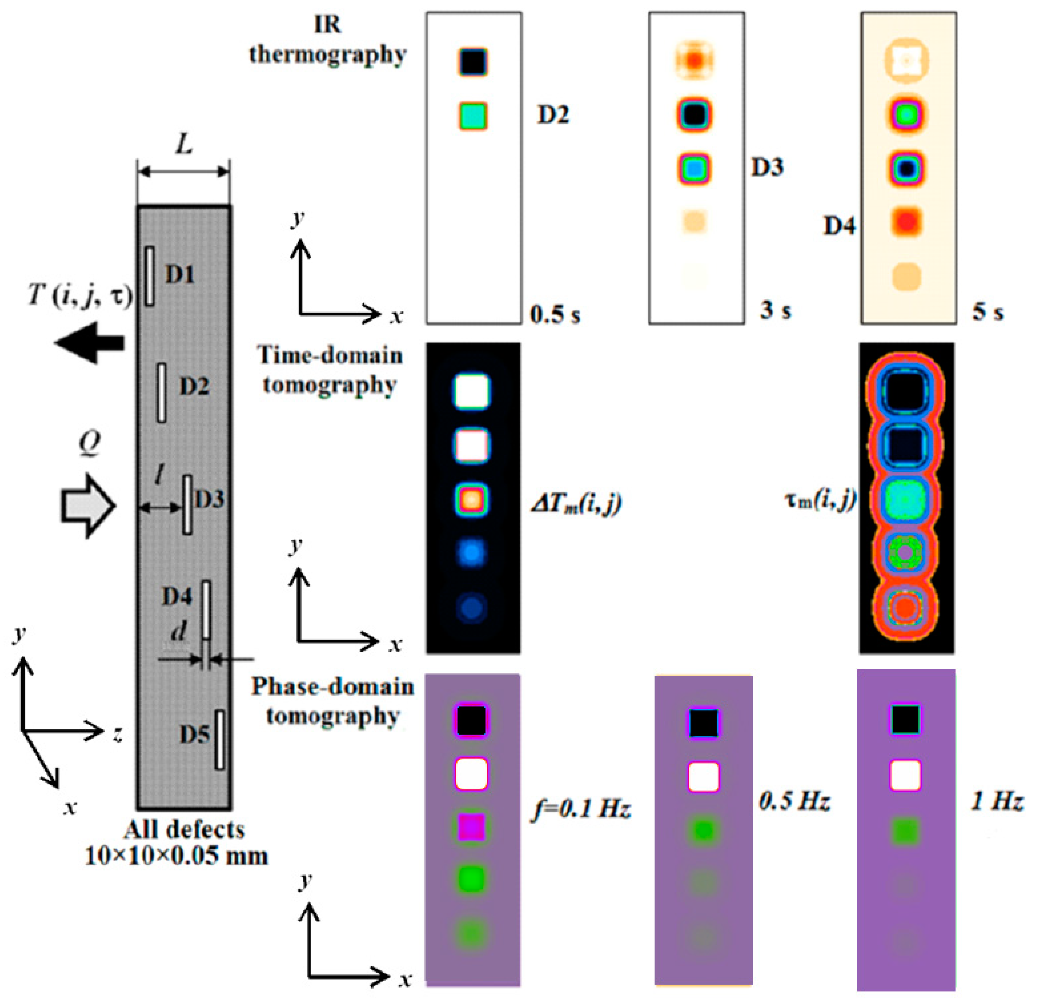
Various aspects of active TNDT have been investigated by using analytical solutions to the heating of one-, two-, or three-layer samples [13,16,17,18,19,20,21]. However, such solutions are simplified and can hardly be applied to practical test situations. Let us illustrate some peculiarities of time/phase tomographic data treatment on a 3D model of 10 × 10 × 0.05 mm air-filled defects located in a 3 mm-thick isotropic CFRP plate, at the depths of 0.1, 0.5, 1.475, 2.45, and 2.85 mm (Figure 1). Note that the defects are located symmetrically off both the front and rear sample surface. The sample is heated with a heat pulse (duration 10 ms, heat power 106 W/m2), and the thermal process is followed for 10 s with an acquisition interval of 10 ms. Calculations were performed by using the ThermoCalc-3D software from Tomsk Polytechnic University, resulting in image sequences including N = 1000 IR thermograms each. The image format was 270 × 70 pixels with the lateral spatial step being 0.5 mm. From the point of view of the classical theory of heat conduction, such a TNDT model represents a multi-layer (up to 36 layers in ThermoCalc-3D) parallelepiped-like sample containing several parallelepiped-like defects (up to 40 defects in ThermoCalc-3D). The side surface of the sample is adiabatic while the front surface is heated with a square heat pulse. Both front and rear surfaces exchange energy with the ambient by convection. On the layer/layer and layer/defect boundaries, there are conditions of continuity of temperature and heat flux. The features of such a TNDT model have been thoroughly discussed elsewhere [13,16,17,18].
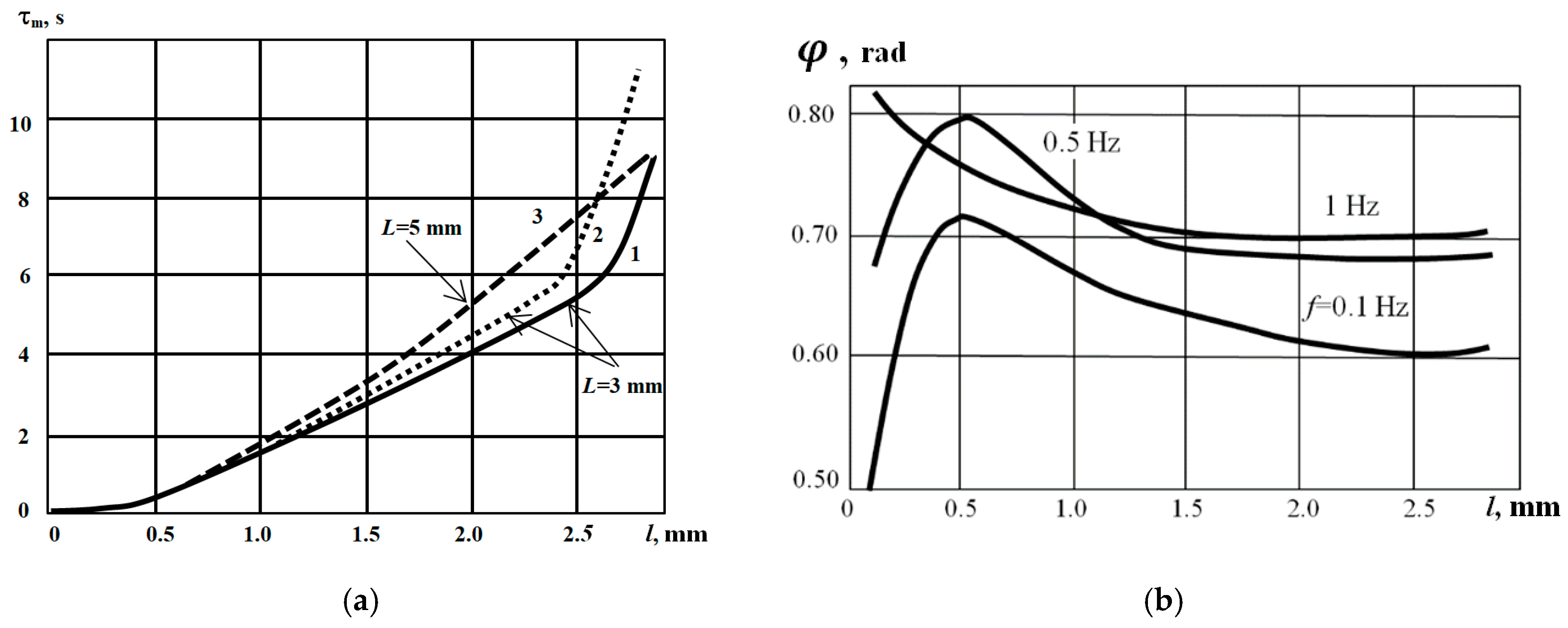
Figure 2 shows two important relationships associated with the above-mentioned test case. Optimum observation time grows up for deeper defects (Figure 2a) and allows for unambiguous evaluation of material layer coordinates . Note that the slope of the sharply increases if defects are located close to the sample rear surface, i.e., where defect depth l and sample thickness L become close (see the curve 1 for L = 3 mm). This conclusion has been confirmed by analytically modeling a 0.1 mm-thick 1D, i.e., laterally-infinite, defect (see the curve 2 in Figure 2a). Calculations have been performed by using the solution for a three-layer non-adiabatic plate heated with a square heat pulse [18]. The dependence of the Fourier phase on defect depth is more complicated, as shown in Figure 2b. The curve shape depends on thermal wave frequency and might have some extremums. This reflects the fact that finite-size defects can be detected in a particular layer by applying a thermal wave of a proper (optimal) frequency. Respectively, the calibration of layer coordinates by phase intervals is difficult. We believe that the phase-domain tomography allows for the improvement of defect visibility but can scarcely be applied for quantitative evaluation. Note also that one should optimally choose not only a phase interval but also a thermal wave frequency. A deeper approach to characterizing defects by phase, based on the concept of a “blind frequency”, was described in [3]. In fact, for each defect depth , one can determine a limiting (“blind”) frequency and any frequency higher than allows no defect detection.
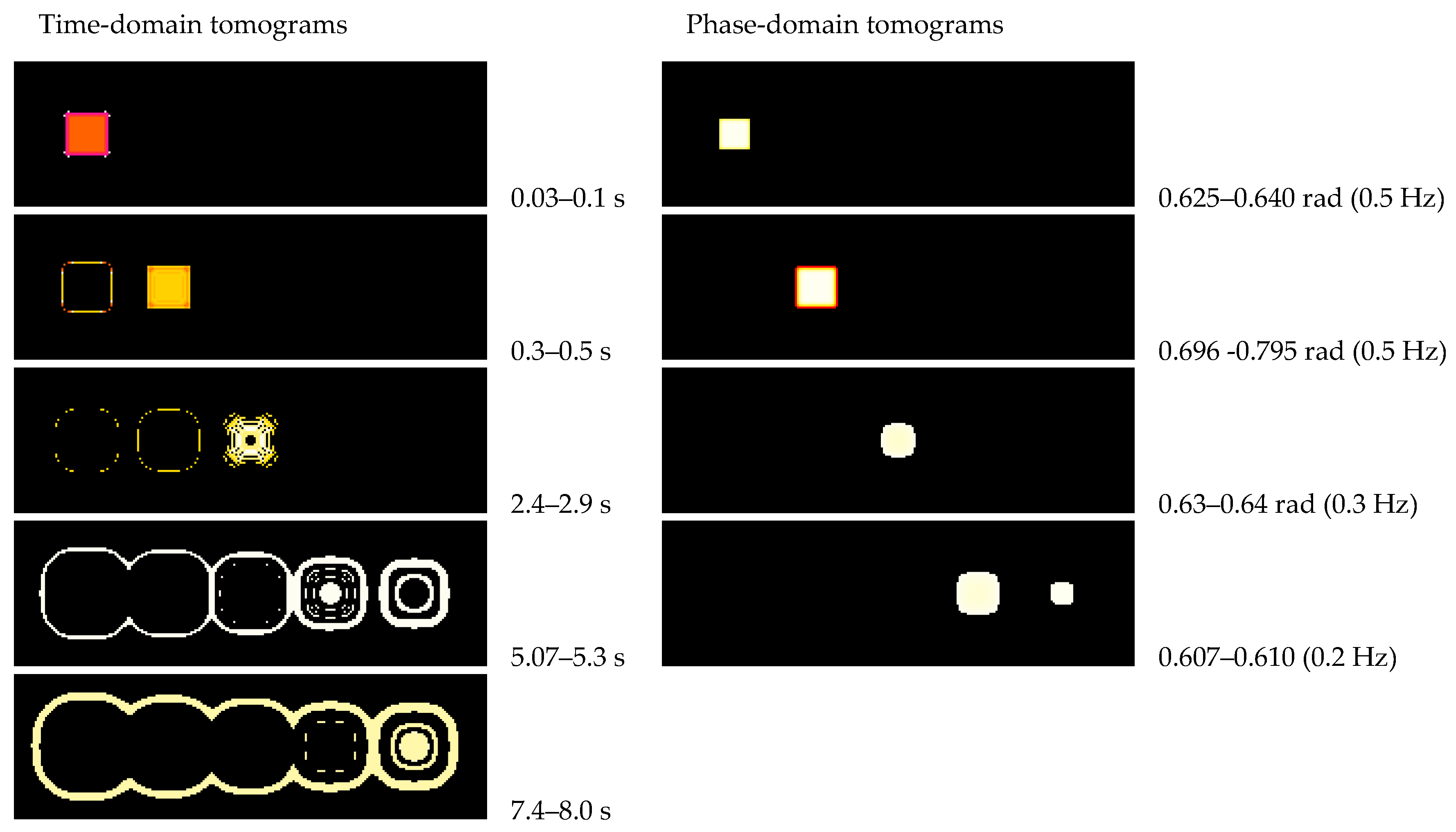
The images in Figure 1 comparatively show collected (raw) IR images and the results of time/phase data treatment. IR images illustrate the gradual appearance of the indication s from the defects located at increasing depths that is a basic phenomenon in active TNDT. As mentioned above, each defect reaches a maximum value at a particular time, thus resulting in the corresponding maxigram and timegram. An important feature of timegrams is the presence of artifacts as round-shape signals surrounding defect indications. These artifacts are conditioned by the fact that some points around shallower defects are characterized by the same values as some deeper defects (see below the discussion on Figure 3 and Figure 4). Hence, thermal tomograms of deeper layers may contain some “footprints” of shallower defects [2,13] (see the time-domain tomography results in Figure 3). It is also worth reminding another unpleasant feature of the time-domain tomography, namely, the necessity of choosing a reference point close to an area of interest. Note that, since the modeling has been fulfilled without taking into account a possible phenomenon of uneven heating, in synthetic images, a reference point can be chosen at any defect-free point. The Fourier transform applied to the raw IR image sequence results in phasegrams (Figure 3) associated with 500 frequencies (if N = 1000) along with the images of Fourier magnitude, known as “ampligrams” (not shown in Figure 3). The important feature of phasegrams is the absence of both a reference point and artifacts. The latter fact means that, in the phase-domain thermal tomography, one may expect clearer images of hidden defects to compare to the time-domain approach. However, it is worth noting that defects located close to the sample rear surface reveal a very small shift in phase , therefore, the defects D4 and D5 cannot be resolved, as shown in the corresponding phasegram-based tomograms (Figure 3). Another problem related to the Fourier transform is that its results depend on the acquisition interval and the number of images in the sequence . Thus, the -th image corresponds to the frequency:
The lowest meaningful frequency, except zero, is:
And the highest frequency in a sequence is:
The above-mentioned peculiarity of the time-domain treatment makes quantitative interpretation of phase data difficult.
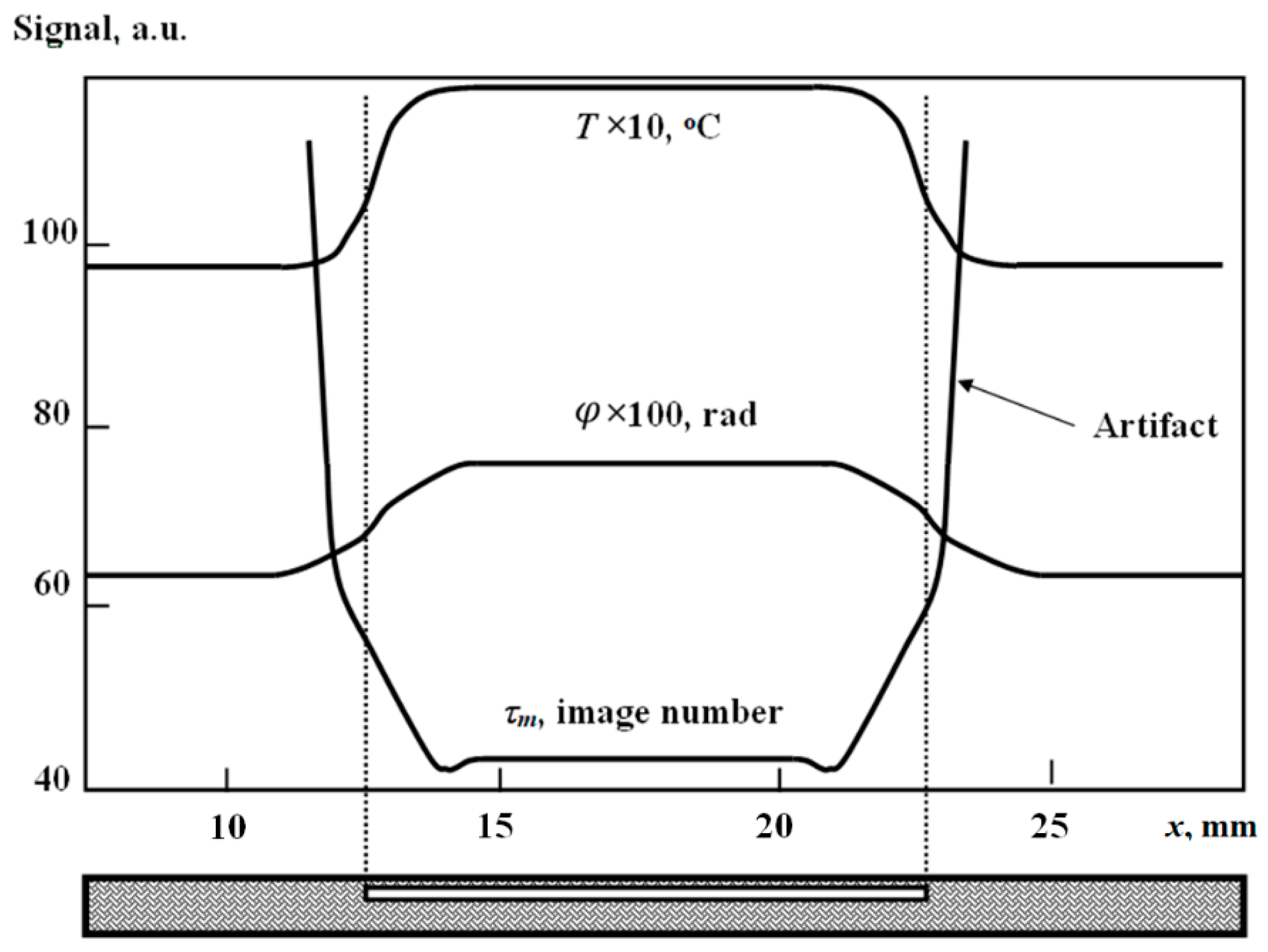
Some features of the approaches above are illustrated in Figure 4 where the spatial profiles of temperature (raw image), characteristic time τm (timegram), and phase (phasegram), over the defect D2 (depth 0.5 mm), are presented. It appears that the profiles of temperature and phase look similarly with the signal plateau over the defect projection. This means that the 10 × 10 × 0.05 mm defect at the depth of 0.5 mm in CFRP can be considered as 1D, and heat diffusion takes place only at the defect borders where the signals decrease by 70% in regard to their maximal value over the defect center. The corresponding profile of τm is also characterized by the plateau but the behavior of this parameter is more complicated due to the fact that timegrams represent a non-linear result of processing raw thermograms. The values of τm, first, slightly drop in the areas where lateral heat diffusion starts, then, increase as values diminish up to zero in defect-free areas. Experimentally, in non-defect areas, τm acquire random values from 1 to N because of a noisy character of signals. The noise can be either experimental or computational depending on whether experimental or synthetic images are processed. This peculiarity of producing timegrams causes round-shaped artifacts around defects when choosing particular intervals, as seen in Figure 3. The fact that signals tend to zero far from defects is used for thresholding τm profiles. In other words, the pixel values in thermal tomograms are set to zero, where the values in the corresponding maxigrams become lower than a chosen threshold , thus allowing clear “footprints” of defects. Unfortunately, there is no definite rule on how to choose the threshold, however, in many cases it is about a few percent of a maximum ΔTm value in the corresponding maxigram.
3. Experimental Setup and Test Samples
In the experimental section of this study, we have used a standard TNDT setup including two Bowens flash lamps with the energy of 1.2 kJ each and a FLIR 625 IR imager. The flash duration was about 10 ms while the acquisition frequency was 10 Hz, with the total number of recorded thermograms being from 200 to 300 in a single test. The tomographic data processing was accomplished by means of the “Thermal tomography” option included in the ThermoFit Pro software from Tomsk Polytechnic University. The corresponding procedure includes choosing a reference point by the thermographer, calculating maxigrams and timegrams and, finally, producing thermal tomograms of some chosen layers including the optimization of a noise threshold by trial. It is important to mention that performing thermal tomography requires a certain experience from the thermographer. In fact, the experimental setup is intended for the personnel certified by Level II or III in TNDT. While using the option of time-domain tomography, one has to determine a calibration relationship by modeling and choose a proper reference point (close to an area suspected as a defect indication). Such calibration relationships are to be defined for particular materials being related to material diffusivity. They are slightly dependent on defect size and thickness, therefore, the values of layer coordinates reported below are approximate. The Fourier transform can be fulfilled in an automatic way because, in most cases, the resulting image is the phasegram at the first significant frequency. However, in some cases, one should optimize the frequency and heuristically choose a phase interval to underline an area of interest.
The experiments described below have been conducted on CFRP samples made of a unidirectional carbon fiber fabric and standard KPR-150 filling (Russian standard TU 2225-012-93660864-2009) with the following ply layup: [+45/0/−45/0/0/90/0/0/−45/0/+45]3. The samples contained impact damages of varying energy delivered to the sample surface through a 10 mm-diameter spherical impactor. Such defects appear on operating aircraft because of various factors, such as falling tools, strikes by birds and baggage, hailing, etc. Impact damage might be invisible on a damaged surface but occupy a considerable delaminated (cracked) area close to the panel rear surface. If a through-transmission IR test is modeled as a pyramid-like set of thin air-filled voids in a material, it should reveal the familiar butterfly-like shape image on the rear surface that is well seen in ultrasonic tests. However, in practice, one should detect such defects only on an impacted surface by applying a one-sided test procedure.
4. Discussion of Results
The results of tomographic data processing in both the time and phase domains are illustrated by Figure 5, Figure 6 and Figure 7. A one-sided test procedure was applied on both the impacted (front) and opposite (rear) surface. In general, all results are consistent since both algorithms are applied to the same raw data.
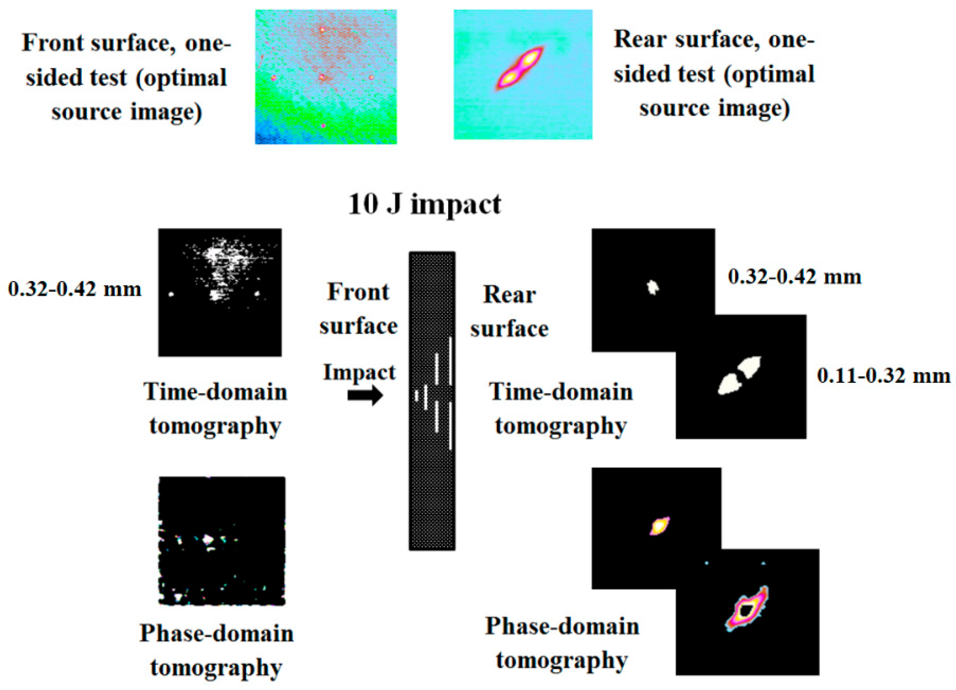
Figure 5 shows results in the case of impact with the energy of 10 J. On the front surface, the phase-domain algorithm was able to detect a faint “footprint” of a butterfly-like delamination, which is clearly detected on the rear surface. The time-domain treatment required thresholding pixel values by , otherwise the tomograms appeared noisy because of artifacts. Oppositely, the phase-domain processing involved the choosing of proper phase intervals in phasegrams without the necessity of defining a reference point and using a threshold. Note that the layer coordinates specified in Figure 5, Figure 6 and Figure 7 were determined by using the calibration relationship from Figure 2 (L = 5 mm) and only in the case of the time-domain tomography, while phase-domain results were not quantified and used to better show the in-depth defect distribution.
When inspecting the sample on the rear surface, the big near-surface delamination (“butterfly wings”) overshadowed smaller defect areas, therefore, only two small symmetrical defects are seen on both time- and phase-domain tomograms (Figure 5).
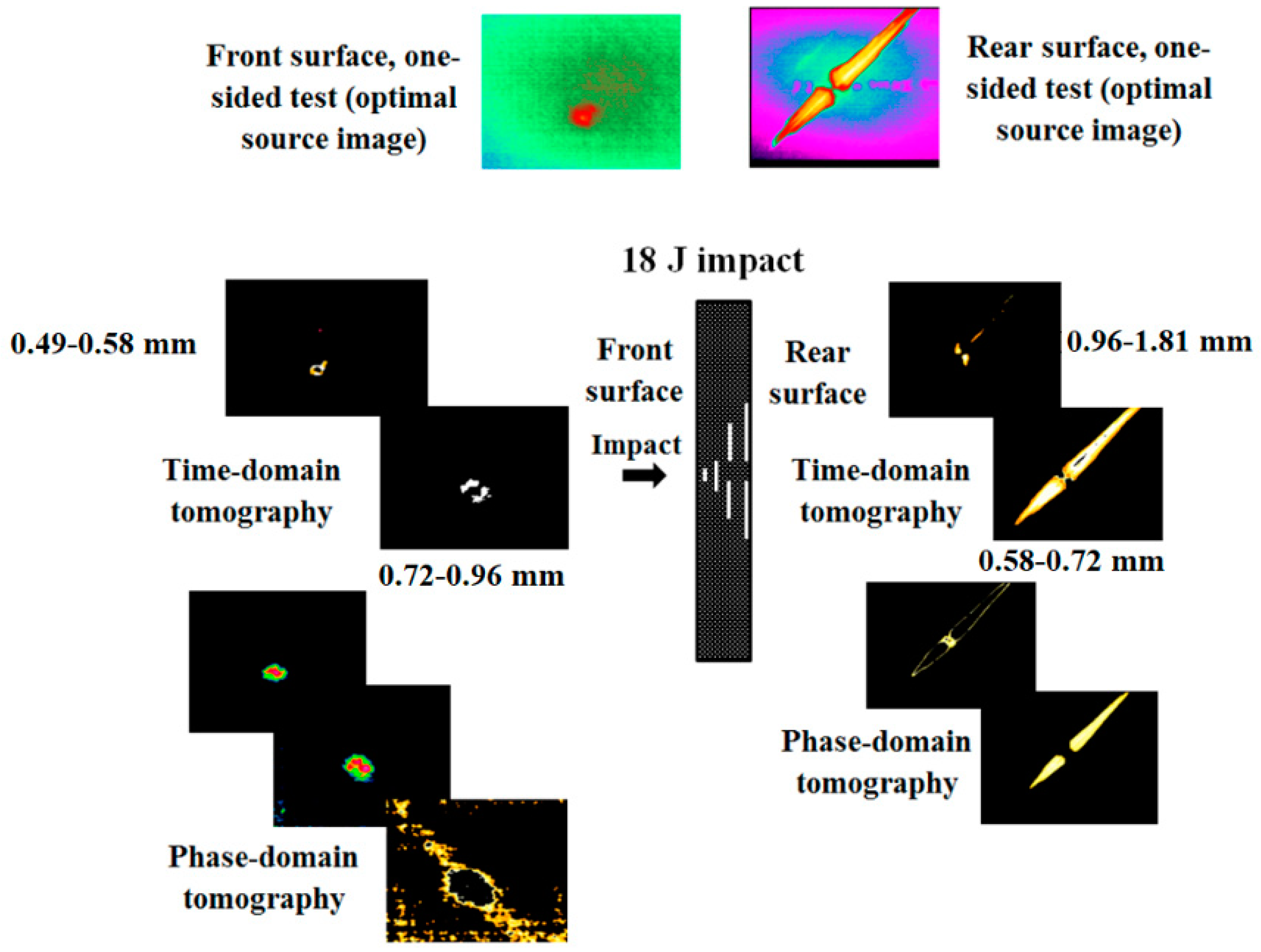
The results obtained on the sample impacted with the energy of 18 J illustrate some typical features of the impact damage detection by using active IR thermography (Figure 6). On the front sample surface, there is hardly any visible material indentation produced by the impact while the main body of the defect appeared close to the rear surface being clearly visible as an evident “butterfly-shape” delamination. The same area is well seen in the front-surface raw image, as well as in the tomograms. The time-domain treatment allowed “slicing” the sample for two layers when analyzing both the front- and rear-surface IR image sequences. Again, it is worth noting that the major delamination, such as seen on the rear surface, overshadows deeper defects, and therefore, a direct comparison of the tomograms obtained in both front- and rear procedures is difficult. However, the results in Figure 6 are similar to those in Figure 5 and illustrate that the main impact energy is absorbed within the CFRP layer adjacent to the sample rear surface to produce the most severe damage of the composite. The phase-domain tomography reveals similar results but the front-surface third tomogram shows the faint indication of the deeper delamination that is unseen in the time-domain tomograms.
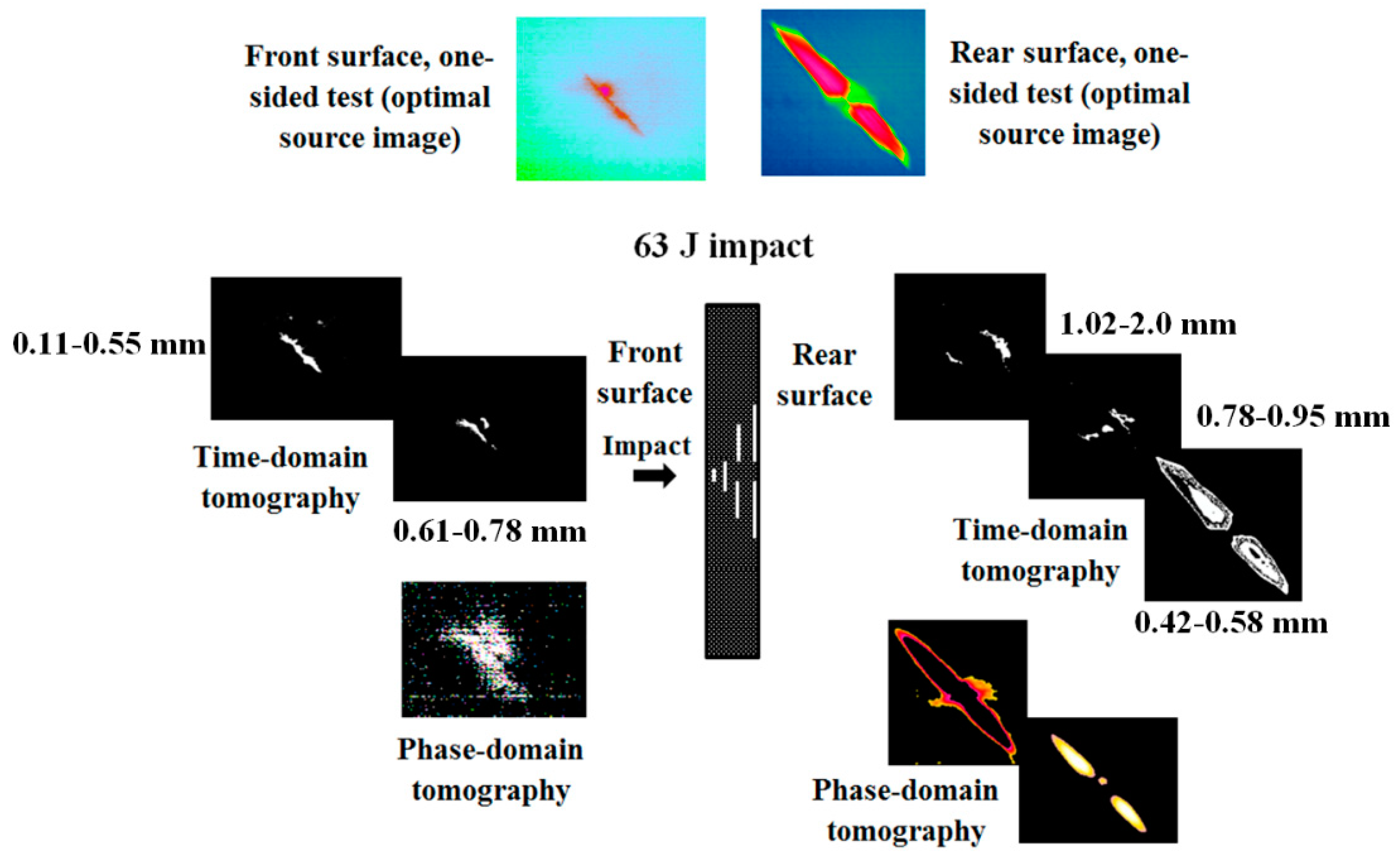
The consequences of the high-energy (63 J) impact seemed to be more devastating for the composite through its whole thickness (Figure 7). The front-surface damage was detected as a surface crack but the tomograms revealed some faint delaminations under the point of impact. Note that the phase-domain tomogram showed a larger damaged area compared to the time-domain data but the time-domain tomography allowed separation of the damaged area into two layers: the superficial one where a thin surface crack was seen, as well as the deeper defect overshadowed by the shallower one. On the rear surface, three time-domain tomograms showed sections of the whole defect located in some layers of the composite characterized by different fiber layup angles. In this test case, the phase tomograms have proven to be less informative in regard to the time-domain images.
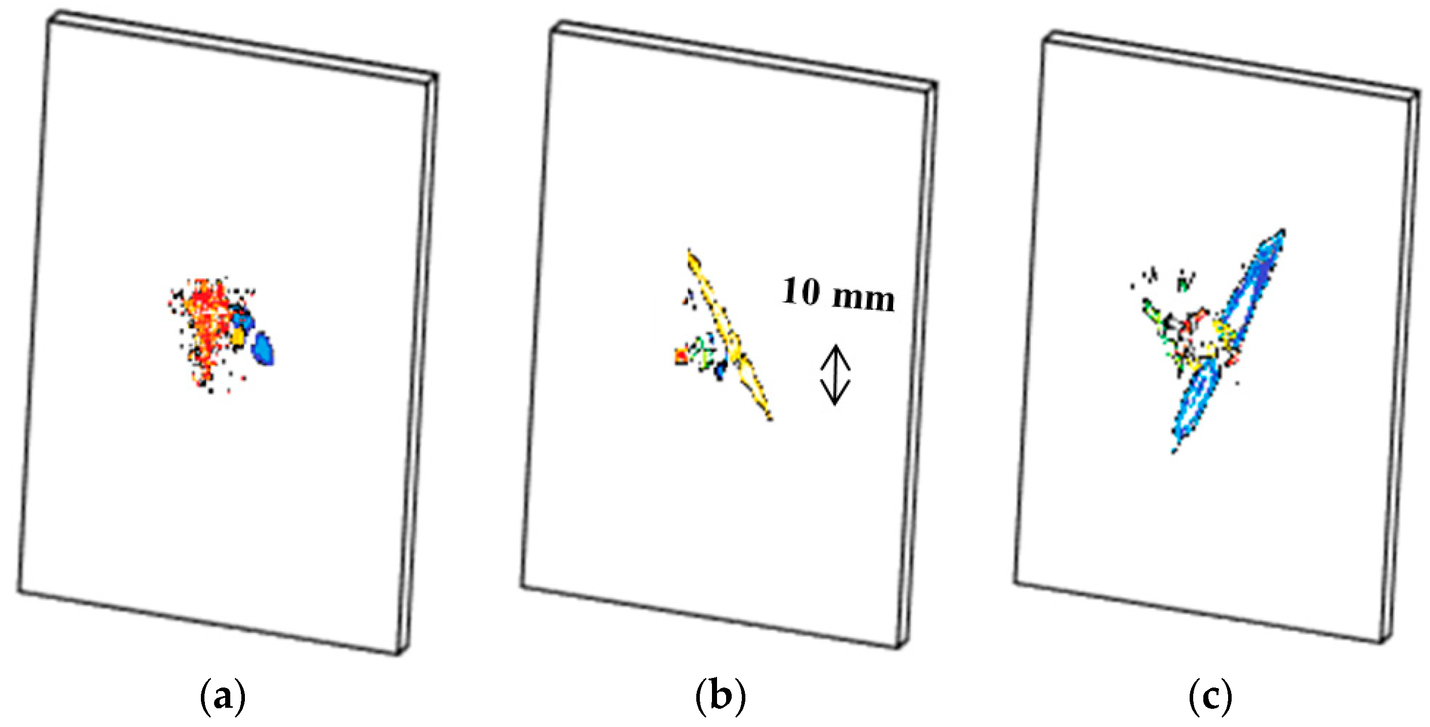
Thermal tomograms can be used for reconstructing complicated defects in solids in a more efficient way to compare to conventional IR thermograms. An example is presented in Figure 8 by using the time-domain data from Figure 5, Figure 6 and Figure 7. The 3D images obtained by superimposing thermal tomograms look illustrative and show depth, planar dimensions and shape of impact damages for three different impact energies. However, these images hardly reflect severity of particular defective areas due to a lack of information on defect thickness, and the depth limit of selected layers is about 2 mm counting from both front and rear sample surface. This is a topic for further research.
5. Conclusions
Thermal tomographic inspection, based on the computer analysis of heat diffusion in solids, is not a common technique, though it competes with the more established X-ray, acoustic and nuclear magnetic resonance techniques. On the one hand, it involves a specialized treatment of the data obtained by means of active IR thermographic NDT, thus allowing for the “slicing” of materials under testing for few (2–3 in our case) layers where discontinuity-like defects can be underlined on the noisy-free background as binary thermal tomograms. From the other hand, this technique still represents an art since its final result depends on thermographers’ skills, even if the very principles of tomographying are well defined. The time-domain tomography is based on the simple fact that, in a one-sided test, the temperature “footprints” of deeper defects appear with time delays in regard to shallower defects. Therefore, selecting a particular time interval is equivalent to choosing planar “slices” within a sample being inspected. The thicknesses of resolved layers increases with layer depth, and, for example, in composites only very shallow plies can be separated by thermal tomography, while, in general, the number of resolved layers is lower than the number of composite plies. By using the Fourier transform in pulsed or thermal wave IR thermographic NDT, one passes into the phase domain where defect temperature indications are associated with phases. There are two specific features that characterize the time- and phase-domain tomographic techniques. The time-domain tomography essentially requires choosing a reference point and, in most cases, such points should be located close to the area of interest, thus making this technique less general. However, time-domain tomograms can be quantified in terms of defect depth, or layer coordinates, thanks to the unambiguous character of calibration relationships. Opposite of this, the phase-domain tomography can be applied to collected IR data in a direct way, but the quantification of results is more difficult because relationships between phase and defect depth depend on experimental parameters and might reveal some extremums, and also an optimal Fourier frequency should be defined. One may state that both the phase-domain data presentation and thermal tomography are heuristically valuable but limited by their qualitative nature.
In this study, the time- and phase-domain thermal tomography techniques have been comparatively applied to the evaluation of the CFRP composite containing impact damage defects characterized by impact energy 10, 18, and 63 J. Both techniques have demonstrated similar results of the reconstruction of thermal tomograms and, in some cases, supplied complementary information about the distribution of single defect areas in the composite. In particular, thermal tomography seems to be useful when performing 3D reconstruction of subsurface defects and studying the severity of damage caused by impacts with varying energy. However, in our case, selected layers have been limited by depth in a CFRP composite of about 2 mm.
Author Contributions
Conceptualization and Methodology, V.P.V.; Software, V.V.S.; Writing—Original Draft, M.V.K.
Funding
This study was supported by Russian Scientific Foundation grant #17-19-01047 (thermal tomography experiments) and Tomsk Polytechnic University Competitiveness Enhancement Program (computer modeling).
Conflicts of Interest
The authors declare no conflict of interest.
References
- Kline, R.A.; Winfree, W.P.; Bakirov, V.F. A new approach to thermal tomography. AIP Conf. Proc. 2003, 22, 682–687. [Google Scholar]
- Vavilov, V.; Maldague, X. Dynamic thermal tomography: New promise in the IR thermography of solids. In Proceedings of the Thermosense XIV: An International Conference on Thermal Sensing and Imaging Diagnostic Applications, Orlando, FL, USA, 22–24 April 1992; pp. 194–206. [Google Scholar]
- Ibarra-Castanedo, C.; Maldague, X. Defect depth retrieval from pulsed phase thermographic data on Plexiglas and aluminum samples. Proc. SPIE 2004, 5405, 348–356. [Google Scholar]
- Rosencwaig, A. Thermal-wave imaging. Science 1982, 218, 223–228. [Google Scholar] [CrossRef] [PubMed]
- Almond, D.P.; Patel, P.M. Photothermal Science and Techniques; Chapman & Hall: London, UK, 1996; p. 241. [Google Scholar]
- Mulaveesala, R.; Tuli, S. Theory of frequency modulated thermal wave imaging for nondestructive subsurface defect detection. Appl. Phys. Lett. 2006, 89, 191913. [Google Scholar] [CrossRef]
- Mandelis, A. Theory of photothermal wave diffraction tomography via spatial Laplace spectral decomposition. J. Phys. A Math. Gen. 1991, 24, 2485. [Google Scholar] [CrossRef]
- Munidasa, M.; Mandelis, A.; Ferguson, C. Resolution of photothermal tomographic Imaging of sub-surface defects in metals with ray-optic reconstruction. Appl. Phys. 1992, 54, 244–250. [Google Scholar] [CrossRef]
- Winfree, W.P.; Plotnikov, Y.A. Defect characterization in composites using a thermal tomography algorithm. In Review of Progress in Quantitative Nondestructive Evaluation; Thompson, D.O., Chimenti, D.E., Eds.; Kluwer Academic Plenum Publishers: Dordrecht, The Netherlands, 1999; Volume 18, pp. 1343–1350. [Google Scholar]
- Toivanen, J.M.; Tarvainen, T.; Huttunen, J.M.J.; Savolainen, T.; Orlande, H.R.B.; Kaipio, J.P.; Kolehmainen, V. 3D thermal tomography with experimental measurement data. Int. J. Heat Mass Transf. 2014, 78, 1126–1134. [Google Scholar] [CrossRef]
- Sun, J.G. Method for Implementing Depth Deconvolution Algorithm for Enhanced Thermal Tomography 3D Imaging. U.S. Patent No. 8465200, 2013. [Google Scholar]
- Sun, J.G. Quantitative three-dimensional imaging of heterogeneous materials by thermal tomography. J. Heat Transf. 2016, 138, 112004. [Google Scholar] [CrossRef]
- Vavilov, V.P. Dynamic thermal tomography: Recent improvements and applications. NDT & E Int. 2015, 71, 23–32. [Google Scholar]
- Zhang, X. Instrumentation in diffuse optical imaging. Photonics 2014, 1, 9–32. [Google Scholar] [CrossRef] [PubMed]
- Friederich, F.; May, K.H.; Baccouche, B.; Matheis, C.; Bauer, M.; Jonuscheit, J.; Moor, M.; Denman, D.; Bramble, J.; Savage, N. Terahertz radome inspection. Photonics 2018, 5, 1–10. [Google Scholar] [CrossRef]
- Balageas, D.L.; Krapez, J.-C.; Cielo, P. Pulsed photo-thermal modeling of layered materials. J. Appl. Phys. 1986, 59, 348–357. [Google Scholar] [CrossRef]
- Maillet, D.; Andre, S.; Batsale, J.-C.; Degiovanni, A.; Moyne, C. Thermal Quadrupoles: Solving the Heat Equation through Integral Transforms; John Wiley & Sons Publ.: New York, NY, USA, 2000. [Google Scholar]
- Vavilov, V.P. Thermal/infrared testing. In Nondestructive Testing Handbook; Kluev, V.V., Ed.; Spektr Publisher: Moscow, Russia, 2009; pp. 1–485. [Google Scholar]
- Noethen, M.; Jia, Y.; Meyendorf, N. Simulation of the surface crack detection using inductive heated thermography. Nondestruct. Test. Eval. 2012, 27, 139–149. [Google Scholar] [CrossRef]
- Ibarra-Castanedo, C.; Maldague, X.P. Infrared thermography. In Handbook of Technical Diagnostics: Fundamentals and Application to Structures and Systems; Czichos, H., Ed.; Springer Publ.: Berlin, Germany, 2013; pp. 175–220. [Google Scholar]
- Gao, B.; Woo, W.L.; Tian, G.Y. Electromagnetic Thermography Nondestructive Evaluation: Physics-based Modeling and Pattern Mining. Sci. Rep. 2016, 6, 25480. [Google Scholar] [CrossRef] [PubMed] [Green Version]
Figure 1.
3D modeling and time/phase data processing in the inspection of CFRP (L = 3 mm, defect size 10 × 10 × 0.05 mm, l = 0.1; 0.5; 1.475; 2.45 and 2.85 mm).
Figure 1.
3D modeling and time/phase data processing in the inspection of CFRP (L = 3 mm, defect size 10 × 10 × 0.05 mm, l = 0.1; 0.5; 1.475; 2.45 and 2.85 mm).

Figure 2.
Dependence of optimum observation time τm (a) and thermal wave phase (b). on defect depth l in the inspection of CFRP (CFRP thermal properties: thermal conductivity 0.64 W·m−1·K−1, diffusivity 5.2·10−7 m2·s−1, L = 3 and 5 mm, defect size 10 × 10 × 0.05 mm, 1, 3—numerical modeling, 2—analytical solution).

Figure 3.
Comparison between time- and phase-domain approaches to thermal tomography.

Figure 4.
Comparing spatial profiles of temperature T, characteristic time τm and phase (10 × 10 × 0.05 mm defect at 0.5 mm depth in CFRP; T and values are normalized to make results comparable).
Figure 4.
Comparing spatial profiles of temperature T, characteristic time τm and phase (10 × 10 × 0.05 mm defect at 0.5 mm depth in CFRP; T and values are normalized to make results comparable).

Figure 5.
Time- and phase-domain thermal tomography of impact damage in 5 mm-thick CFRP sample (10 J impact energy).
Figure 5.
Time- and phase-domain thermal tomography of impact damage in 5 mm-thick CFRP sample (10 J impact energy).

Figure 6.
Time- and phase-domain thermal tomography of impact damage in 5 mm-thick CFRP sample (18 J impact energy).
Figure 6.
Time- and phase-domain thermal tomography of impact damage in 5 mm-thick CFRP sample (18 J impact energy).

Figure 7.
Time- and phase-domain thermal tomography of impact damage in 5 mm-thick CFRP sample (63 J impact energy).
Figure 7.
Time- and phase-domain thermal tomography of impact damage in 5 mm-thick CFRP sample (63 J impact energy).


© 2018 by the authors. Licensee MDPI, Basel, Switzerland. This article is an open access article distributed under the terms and conditions of the Creative Commons Attribution (CC BY) license (http://creativecommons.org/licenses/by/4.0/).
Share and Cite
MDPI and ACS Style
Vavilov, V.P.; Shiryaev, V.V.; Kuimova, M.V. Time- and Phase-Domain Thermal Tomography of Composites. Photonics 2018, 5, 31. https://0-doi-org.brum.beds.ac.uk/10.3390/photonics5040031
AMA Style
Vavilov VP, Shiryaev VV, Kuimova MV. Time- and Phase-Domain Thermal Tomography of Composites. Photonics. 2018; 5(4):31. https://0-doi-org.brum.beds.ac.uk/10.3390/photonics5040031
Chicago/Turabian StyleVavilov, Vladimir P., Vladimir V. Shiryaev, and Marina V. Kuimova. 2018. "Time- and Phase-Domain Thermal Tomography of Composites" Photonics 5, no. 4: 31. https://0-doi-org.brum.beds.ac.uk/10.3390/photonics5040031
Note that from the first issue of 2016, this journal uses article numbers instead of page numbers. See further details here.