High-Sensitivity Fiber Fault Detection Method Using Feedback-Delay Signature of a Modulated Semiconductor Laser

Abstract

We propose a high-sensitivity fiber fault detection method using the feedback-delay signature of a modulated semiconductor laser. The modulated laser is directed to a fiber fault and then receives the fault echo, which, in principle, forms an external cavity feedback laser. The fault location, i.e., the external cavity length, is measured by the feedback-delay signature appearing on the laser modulation response curve. The resonance effect between the modulation frequency and external cavity frequency significantly enhanced the laser sensitivity to feedback light and then led to highly sensitive fault detection. Numerical simulations based on laser rate equations predicted that −118.1 dB sensitivity to fault echo light can be obtained.

1. Introduction

Fiber fault location is an essential requirement to guarantee communication service in optical communication systems. With the development of optical access networks or ultralong fiber systems that have large insertion loss, high-sensitivity fault detection is required while maintaining long range and high spatial resolution. One typical example is the monitoring requirement of the time-division multiplexing passive optical network. A large number of branches bring a high insertion loss, which requires high sensitivity to respond to the weak fault echo. Meanwhile, the dense fiber distribution needs a high spatial resolution to locate faults within a range of at least 20 km (from 20.1 km to 20.5 km) [1].

Optical time domain reflectometry (OTDR) is the traditional method using the pulse-based time-of-flight principle [2]. This method usually trades off dynamic range against spatial resolution by using a wide pulse light to ensure echo power that can be detected. Using pulse coding, a random pulse sequence or chaotic light [3,4,5,6,7,8,9,10,11,12] can increase the dynamic range without sacrificing spatial resolution, but the sensitivity is also limited by the dark current noise of the photodetector. Using a photon-counting detector can improve the detection sensitivity, but simultaneously results in a large dead zone due to the dead time of photon counting [13].

Optical frequency domain reflectometry (OFDR) using a frequency-swept laser is capable of high resolution and large dynamic range benefiting from coherent detection [14,15,16], and thus can be used to characterize optical components and modules [17,18]. The restriction of OFDR is that the measurement distance is usually limited to about 500 m by the coherence length of the probe laser [14]. It is worth noting that the laser-based self-mixing interferometry [19,20,21,22] uses a laser to receive a part of its own light reflected from a target and then measures the target distance and vibration. This method is also optical coherent detection and has high sensitivity and a limit measure distance.

We noted that a semiconductor laser subjected to external optical feedback can generate a chaotic temporal waveform that has a feedback-delay signature [23]. The delay signature exposes the feedback-delay value, and thus is usually viewed as unfavorable for secure communication and key distribution [24,25,26,27]. In our previous work [28], the feedback-delay signature was proposed to measure fiber fault. The principle is using the fiber fault as an external reflector to form optical feedback to a laser and then measuring the feedback-delay signature to realize fault location. The delay signature exists both in coherent and incoherent feedback scenarios [29,30], and thus leads to the capability of long measurement distance. However, a certain feedback strength is required to induce laser chaos, and thus the sensitivity is limited to approximately −50 dB [31].

In this paper, we propose and numerically demonstrate high-sensitivity fiber fault detection using the feedback-delay signature of a modulated semiconductor laser. By utilizing the resonance effect between the modulation frequency and external cavity frequency, one can obtain the feedback-delay signature even when the feedback is so weak that the laser is still static. The delay signature will appear on the modulation response function of the laser with optical feedback [32], and thus can be obtained by calculating the inverse Fourier transform (IFT) of the modulation response function. Simulation results predicted that the sensitivity to the feedback strength of this method has the potential to reach −118.1 dB with the optimization of laser parameters and modulation parameters.

2. Methods

2.1. Principle

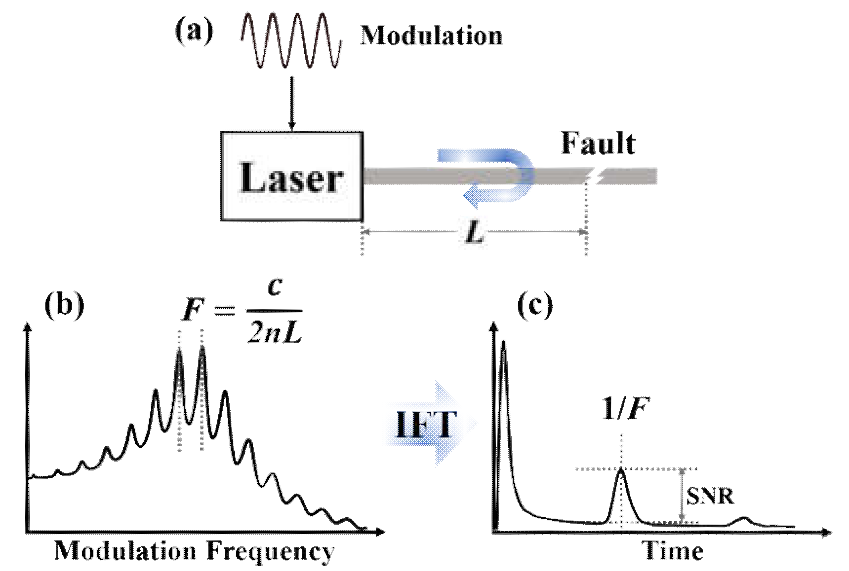
The principle of the frequency resonance method is shown in Figure 1. The modulation signal of frequency f_m is directly added on the bias current of the laser, and the laser emits the light to the fiber under test, as shown in Figure 1a. At this time, the amplitude of the laser output power is the response at the modulation frequency f_m. The modulation response curve of the semiconductor laser is obtained by sweeping the frequency and then recording the response at different frequencies. When the fiber fault occurs, a reflection from the fault will feed back to the laser, and a high or low response will appear that is different from the modulation response without feedback, as shown in Figure 1b. The fluctuation period is inversely proportional to the fault distance L, e.g., F = c/2nL. By calculating the inverse Fourier transform (IFT) of the modulation response curve, one can obtain a clear peak located at t = 1/F, as plotted in Figure 1c. Thus, this peak reads out the position of the fiber fault, which we named “feedback-delay signature” (FDS), referring to the time-delay signature.

Obviously, the delay peak in the IFT curve is the manifestation of the final result for the frequency resonance method, and the identification of the FDS becomes an important factor for fault location. In order to facilitate the analysis of the apparent degree of the FDS, we define the ratio of the FDS level to nearby noise level as signal-to-noise ratio (SNR), and when the SNR decreases to 3 dB, we regard the FDS as unable to be recognized.

2.2. Theoretical Model

The theoretical model of the DFB laser is based on the Lang–Kobayashi rate equations. In order to investigate the theoretical limit of sensitivity that can be achieved by this method, the spontaneous radiation noise of the laser is not considered in the rate equation. Rate equations are shown as follows:

$$\frac{dA\left(t\right)}{dt}=\frac{1}{2}\left\{\frac{\Gamma G_n\left[N\left(t\right)-N_0\right]}{1+\epsilon A^2\left(t\right)}-\frac{1}{{\tau }_p}\right\}A\left(t\right)+\frac{k}{{\tau }_{in}}A\left(t-\tau \right)\cos \theta \left(t\right)$$

(1)

$$\frac{d\varphi \left(t\right)}{dt}=\frac{1}{2}\alpha \left\{\frac{\Gamma G_n\left[N\left(t\right)-N_0\right]}{1+\epsilon A^2\left(t\right)}-\frac{1}{{\tau }_p}\right\}-\frac{k}{{\tau }_{in}}\frac{A\left(t-\tau \right)}{A\left(t\right)}\sin \theta \left(t\right)$$

(2)

$$\frac{dN\left(t\right)}{dt}=\frac{I_m\left(t\right)}{qV}-\frac{N\left(t\right)}{{\tau }_n}-G_n\left[N\left(t\right)-N_0\right]A^2\left(t\right)$$

(3)

where A and ϕ are the amplitude and the phase of the electrical field, respectively, and N is the carrier density. Γ is the optical confinement factor, G_n is the gain coefficient, ε is coefficient of gain saturation, and N₀ is the transparent carrier density. τ_n and τ_p are carrier and photon lifetime, respectively. The round-trip time in the laser internal cavity is τ_in. The amplitude feedback coefficient is k = (1 − r₀²)r/r₀, where r and r₀ are the amplitude reflectivity of the fiber fault and the laser facet, respectively. We define the intensity reflectivity of the fault as feedback strength and denote it as R = 10log(r²) in dB. The feedback phase θ(t) = ωτ + f (t) − f (t−τ), and τ = 2nL/c is the round-trip time of light between the laser facet and the fiber fault located at a distance L, where ω, n, and c are the angular oscillation frequency, the refractive index of fiber, and the velocity of light in vacuum, respectively. The symbols of linewidth enhancement factor, the electron charge, and the internal cavity volume of the laser are defined as α, q, and V. The modulation current I_m(t) = I_b + M(I_b − I_th)cos(2πf_mt), where I_b and I_th are the bias and threshold current, and M and f_m are the modulation depth and modulation frequency, respectively.

The values of all the parameters in our simulation are described as follows: Γ = 0.24, G_n = 5.89 × 10⁻¹² m³/s, N₀ = 0.455 × 10²⁴ m⁻³, ε = 5 × 10⁻²³ m³, τ_n = 2.5 × 10⁻⁹ s, τ_p = 1.5 × 10⁻¹² s, τ_in = 7 × 10⁻¹² s, α = 5, V = 3.24 × 10⁻¹⁶ m³, r₀ = 0.55, ω = 1.216 × 10¹⁵ rad/s, q = 1.602 × 10¹⁹ C, and I_th = 19 mA.

3. Results

3.1. Sensitivity

In our simulation, we set τ at 11 ns and the bias current at 2I_th. Under this bias current condition, the output power of the laser is much less than the laser-induced damage threshold. Even if 100% of the feedback optical power is added, the optical power inside the laser is still less than the laser-induced damage threshold. Lasers will not be destroyed by the tiniest amounts of light feedback. The relaxation oscillation frequency f_r of the laser is around 3.6 GHz. Due to the modulation response curve of the laser without feedback having a Gaussian-like shape, we set the modulation frequency sweeping area as 0–20 GHz to cover the whole response frequency. Even if the increasing bias current will make the f_r of the laser increase, it is still confined within the sweeping range. Considering the large-signal modulation maybe dominating the laser output oscillation in excessive amplitude and causing difficulty in finding the resonance phenomenon, we used small-signal modulation and set M at 0.05. We initially used 10 MHz as the frequency sweeping step to balance the modulation scanning speed and the fineness of the modulation response curve.

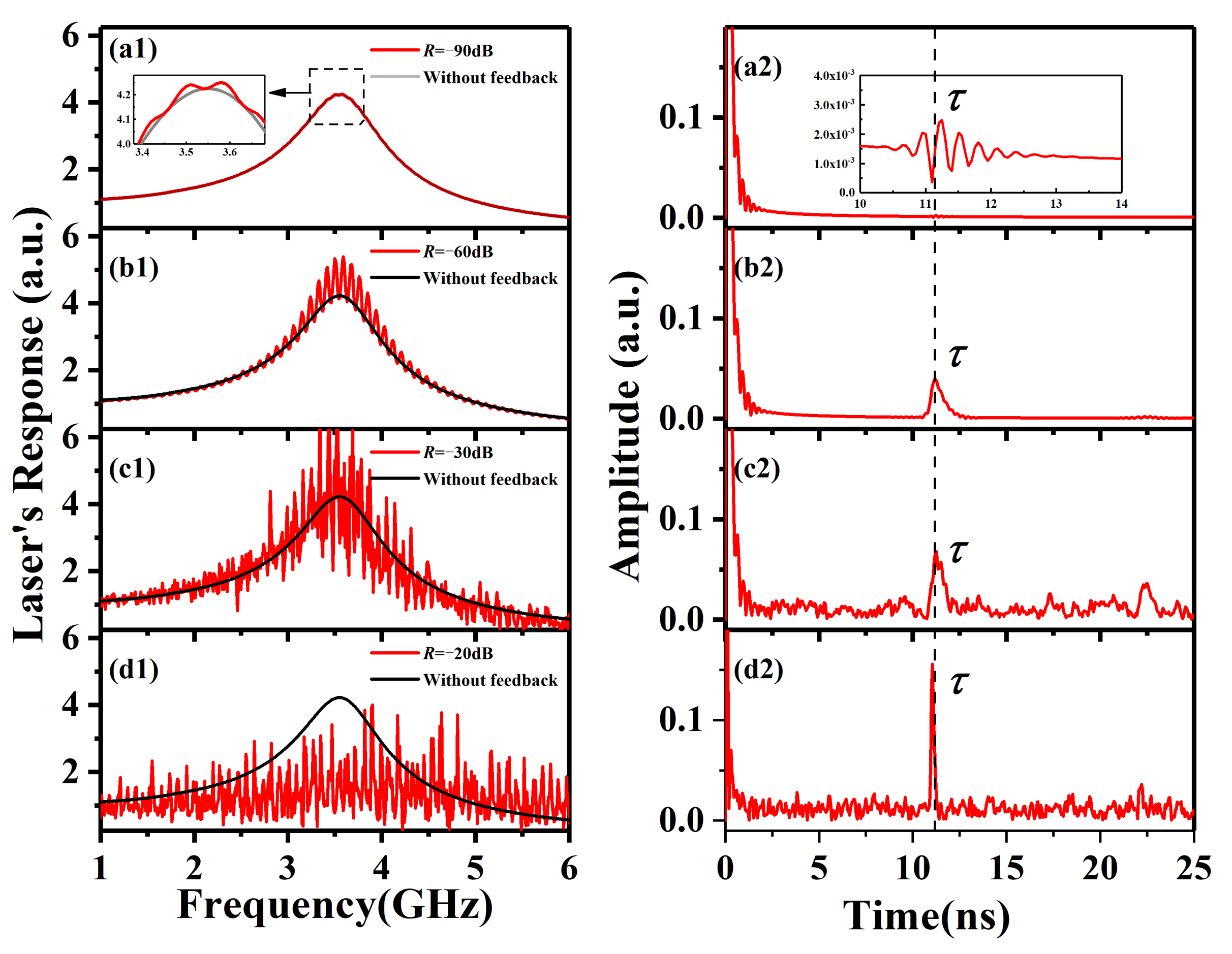
As shown in Figure 2(a1), when R is lower than −90 dB, the modulation response curve (red) is almost coincident with the curve without feedback (gray). Only a slight fluctuation can be found when the curve is zoomed in and examined carefully, as shown in Figure 2(a1) and the inset. A tiny FDS is also hard to see around the 11 ns position in the IFT curve, which is plotted in Figure 2(a2). Continuing to increase the feedback strength (up to −60 dB), the periodic fluctuations on the modulation response curve become obvious, as shown in Figure 2(b1). The FDS shows up prominently above the noise level at 11 ns, which is shown in Figure 2(b2). When the value of R changes to −30 dB, a muddled fluctuation appears and influences the period intuitive identification in the modulation response curve, as shown in Figure 2(c1). In the corresponding IFT result (Figure 2(c2)), the noise floor is not smooth, as mentioned above, and the FDS peak not only appears at the right position but also at 2τ. As shown in Figure 2(d1), strong feedback at R = −20 dB will make the modulation response fall to the bottom, and the muddled fluctuation is still too strong to cover up the period oscillation. However, when using IFT to extract the period, as in Figure 2(d2), one can see that the level of FDS becomes more significant above the thick noise floor.

In realistic scenarios, we can use a network analyzer to measure the modulation response curve of the laser. One port of the network analyzer is connected to the modulation port of the laser to provide the modulation signal. The other port is connected to a photodetector to receive the direct output of the laser. There are three possible sources of noise during the measurement of modulated response curves. The first one is the spontaneous radiation from the laser, the second one is the photodetector dark current, and the last one is the network analyzer measurement error. Among them, the measurement error of the network can be reduced by calibration, and the photodetector dark current and the spontaneous radiation noise of the laser can be reduced by filters. Therefore, the effect of noise in the measured modulation response curve will not be significant, so the effect of noise on the SNR is not significant.

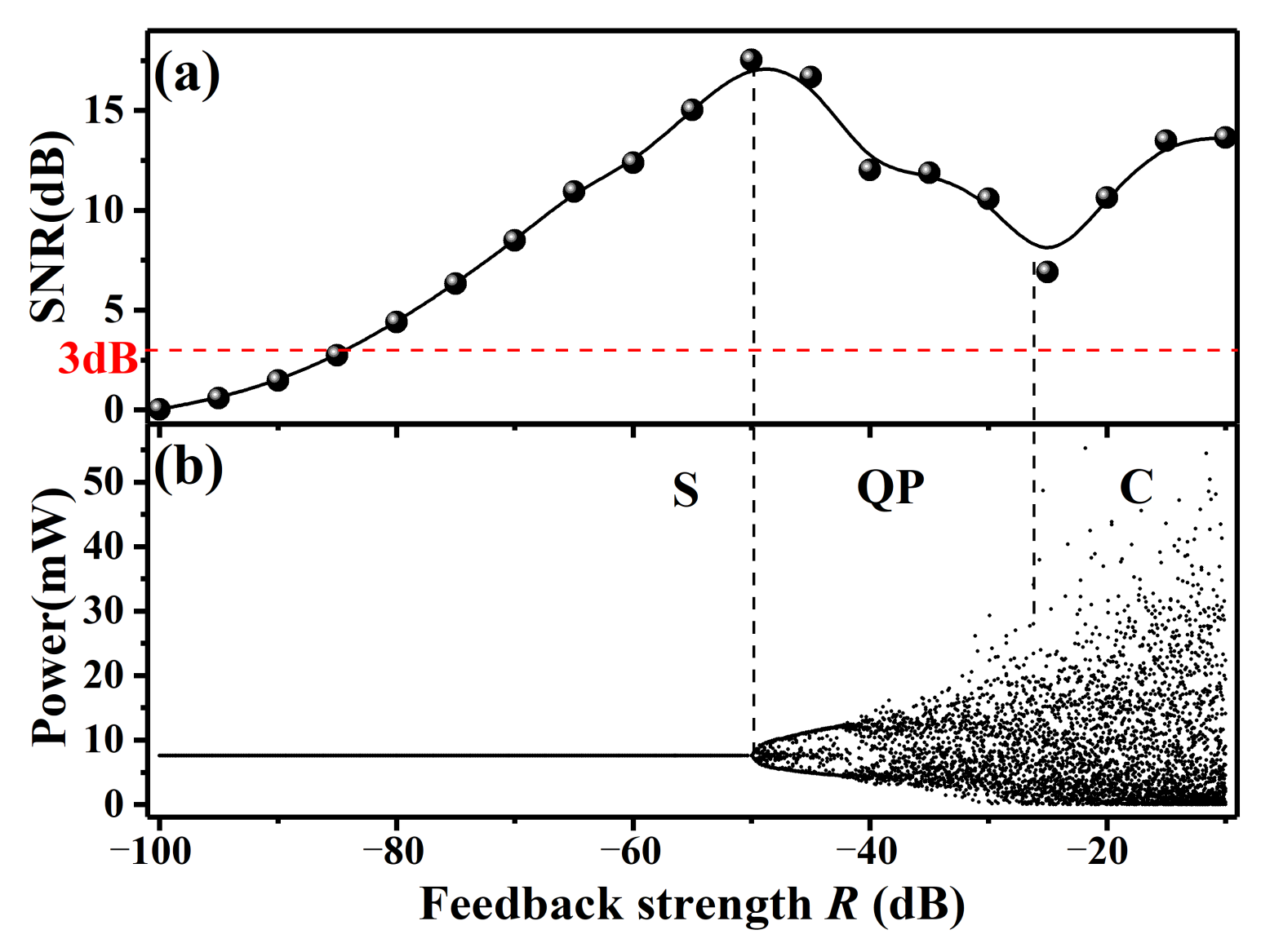
We illustrate the effects of R on the SNR under I_b = 2I_th in Figure 3a. The SNR rises with the R increase and reaches the maximum at R = −50 dB. After that, the SNR decreases until R increases to −25 dB, and then increases again when R continues to increase. According to the criterion of 3 dB, the sensitivity of the frequency-resonance method is −84.3 dB with the laser running at 2I_th bias current.

The tendency of SNR change versus R is attributed to the nonlinear dynamic states of the laser under different R. Figure 3b shows a bifurcation diagram to investigate the dynamic state evolution of the laser without modulation. The bifurcation diagram is obtained from a time series by sampling and plotting local peaks and valleys of the waveform with variable R. The first bifurcation occurs at R = −50 dB, where the laser output state changes from stable (S) to quasi-periodic (QP). This value just corresponds to the turning point of the SNR curve in Figure 3a and explains the reason for SNR changing. In a stable state, the resonance effect between modulation frequency and external cavity resonant frequency dominates the period fluctuation in the modulation response. When the laser output is in the QP state, the large value of the period influences the independence of FDS in the IFT curve, causing a decrease in SNR. However, the time-delay signature of chaos weakens the influence of other periods and combines with the resonance effect to enhance the FDS when the laser enters chaos state (C). That is why the SNR will rise again after R = −25 dB.

As we know, the bias current will influence the f_r, and the modulation response also changes accordingly. Figure 4a shows the modulation response subject to R = −60 dB under different bias current. Obviously, with the bias current increasing, f_r, which is indicated by the maximum position in the modulation response curve, moves to the higher frequency, with the peak level decreasing. Moreover, the period fluctuation also shows a shrinking trend, which is shown in the inset of Figure 4a. The amplitude of period fluctuation decreases from 0.7 at 2I_th to 0.035 at 10I_th. Corresponding IFT curves are illustrated in Figure 4b. The FDS level changes with the increasing bias current, and the highest value appears at I_b = 2I_th. The inset shows the variation in SNR, and the SNR decreases from 13.4 dB to 10.1 dB when I_b increases from 2I_th to 10I_th. Apparently, the sensitivity of the frequency resonance method will change with the difference in SNR under different I_b. As shown in Figure 4c, the sensitivity decreases to −74 dB at I_b = 10I_th.

3.2. Sensitivity Improvement Potential

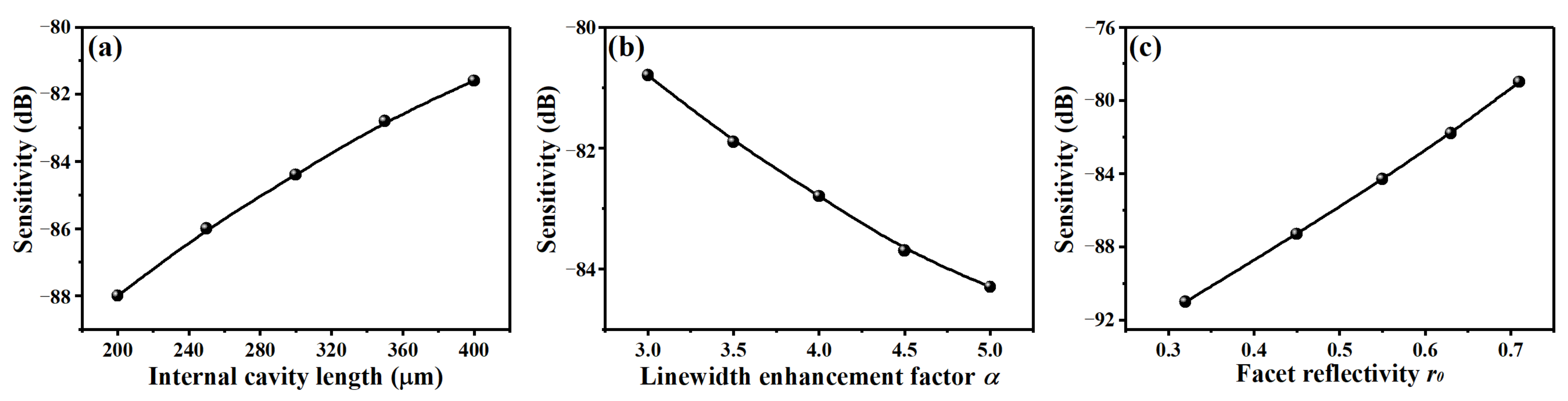
Previous research has indicated that the sensitivity to the feedback strength of a semiconductor laser has a relationship with other internal parameters [33], such as round-trip time in internal cavity τ_in, linewidth enhancement factor α, and facet reflectivity r₀. Therefore, there is still potential to enhance the sensitivity with the frequency resonance method. In order to express the structural parameters of the laser conveniently, here, we used internal cavity length instead of τ_in. The internal cavity length’s influence on the sensitivity is shown in Figure 5a. With the increase in internal cavity length from 200 to 400 μm, the sensitivity almost appears to linearly decrease from −88 to −81.6 dB.

As shown in Figure 5b, the influence of α presents an opposite linear trend to internal cavity length. When the factor is 3, the sensitivity is just −80.8 dB, but the sensitivity enhances to −84.3 dB when α increases to 5. Figure 5c describes the influence of r₀ on the sensitivity of the frequency resonance method, and it also shows a linear trend. When the facet reflectivity is decreased, the sensitivity can reach a high value, to −91 dB and even at 0.7 reflectivity, and the sensitivity just decreases to −79 dB.

3.3. Modulation Parameters

In this section, we analyze the influence of the modulation depth M, frequency sweeping range ΔF, and step Δf on the SNR by setting I_b = 2I_th and R = −60 dB.

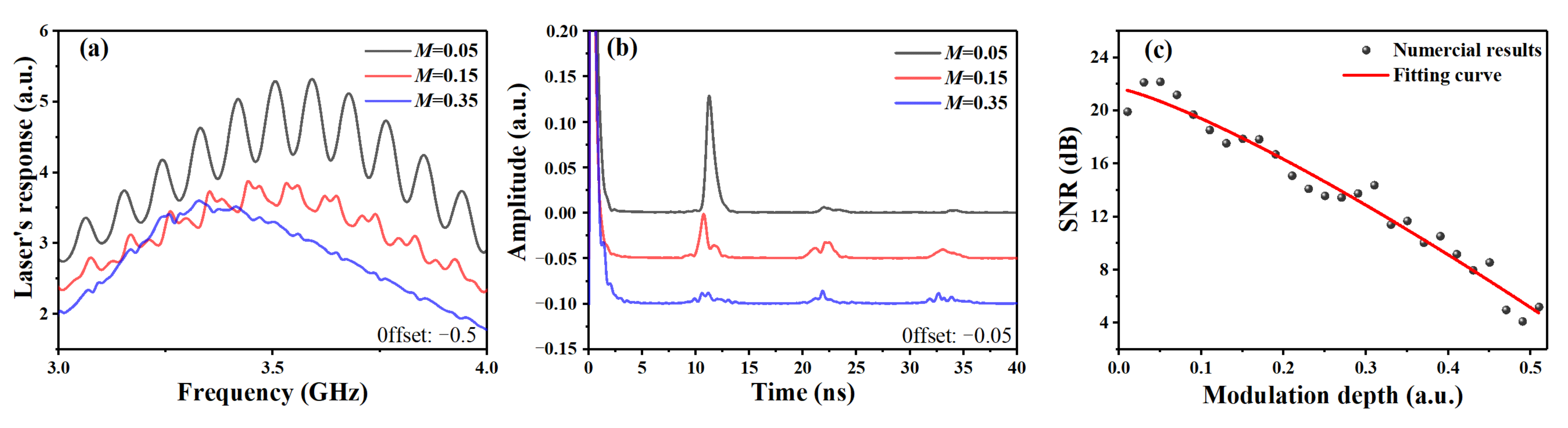
When M is very small at 0.05, the modulation response curve around f_r oscillates smoothly like a sine curve with a stable period. The calculation result of IFT also shows a significant peak at the FDS position. These are the typical results of this method. However, as the modulation depth increases, the modulation response curve and IFT curve deteriorate by harmonic frequencies, which are plotted by red and blue in Figure 6a,b, where the modulation depth is 0.15 and 0.35, respectively. The deterioration also makes the FDS shift left slightly. The trend in Figure 6c shows that the SNR rapidly drops to 4 dB as M increases to 0.5. It is also suggested that the small signal modulation should be kept by setting M < 0.1 to make the SNR higher than 18 dB.

Figure 7 illustrates the effects of frequency sweeping range ΔF on the detection results, which are obtained with optical feedback R = −60 dB. Seen from the modulation response in Figure 7a, the period fluctuation is stronger around f_r. The large fluctuation will achieve more significant FDS. We, thus, choose the frequency sweeping range centered at f_r, as shown in Figure 7a. The corresponding IFT curves are demonstrated in Figure 7b, and the FDS decreases from 0.39 to 0.09, while the ΔF changes from 0.5f_r to 2.5f_r. This decreasing trend can be explained by the large amount of smaller and smaller amplitude period fluctuations on both sides of f_r, which averages the value of FDS.

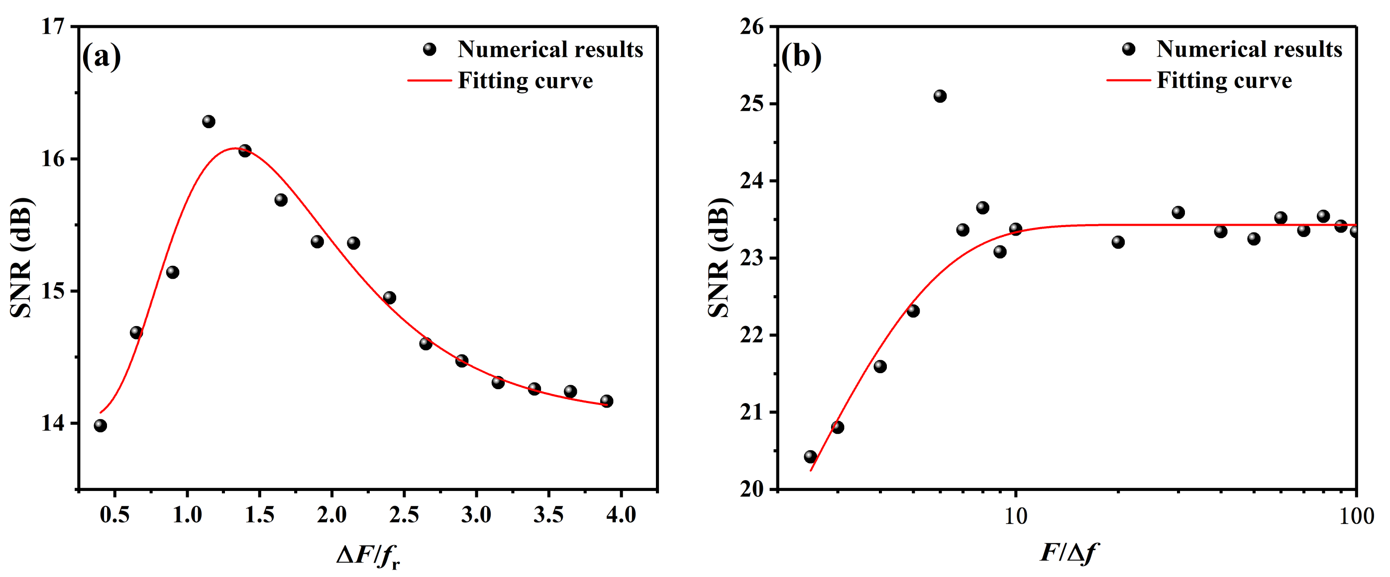
Figure 8a demonstrates the effect on SNR, and it shows a fast rise at the beginning followed by a slowly falling trend. In this result, all SNR values are higher than 13 dB, and the maximum SNR occurs around ΔF = 1.3f_r, corresponding to 4.68 GHz. In addition, Δf of modulation frequency actually acts as a sampling interval of the modulation response curve, and thus there should be an optimum frequency sweeping step when the external frequency F is fixed. Figure 8b shows the SNR as a function of the product F/Δf, which is obtained with ΔF =1.3f_r. The SNR increases first and then becomes stable as F/Δf increases beyond 10, which means ten sampling points are measured in one fluctuation period of the modulation response curve.

Due to the IFT, Δf also limits the detection distance of the modulation resonance method, since the relationship between Δf and the time length ΔT of the time sequence after IFT processing is ΔT = 1/(2Δf). The maximum detection distance L_max of the modulation resonance method is c/(4nΔf).

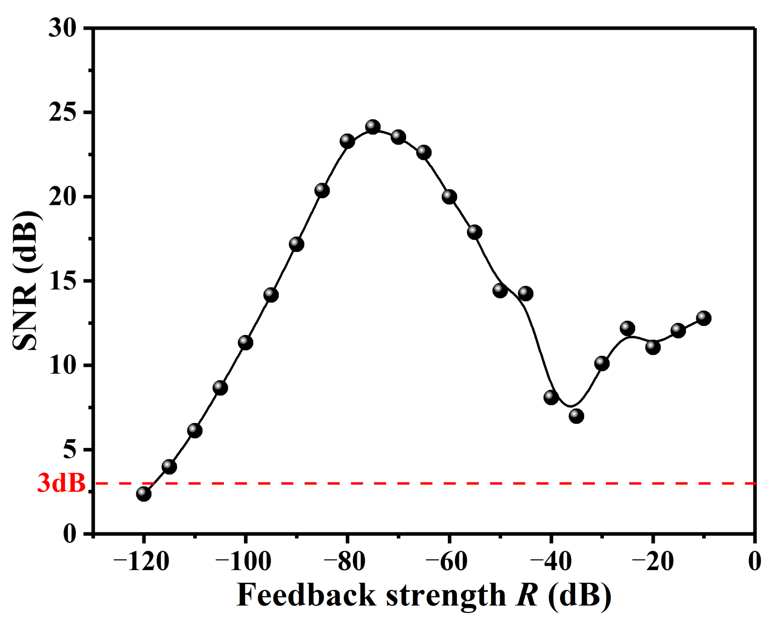
According to the above analysis of the effects of laser and modulation parameters on the SNR, we optimized all parameters to acquire better sensitivity of the frequency resonance method. Figure 9 shows the variation in SNR versus feedback strength, where the parameters set are I_b = 2I_th, α = 5, r₀ = 0.1, 200 μm internal cavity length, ΔF = 4.68 GHz, and Δf = 0.1F, respectively. In this case, the sensitivity reached the highest level at −118.1 dB.

4. Discussion

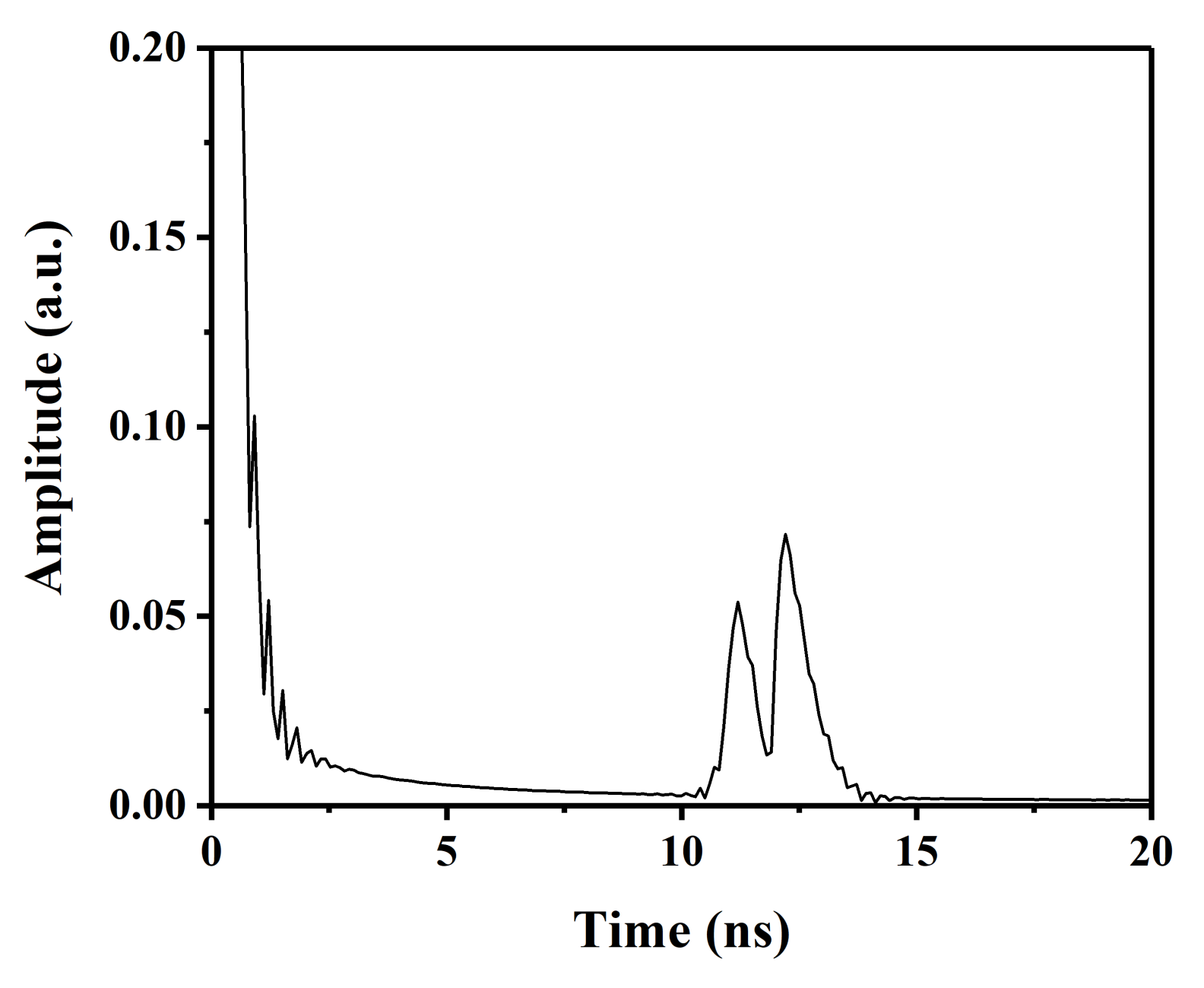
The frequency resonance method can be used to detect reflection events in single-mode fibers. In addition, the method can be used to detect faults in multiple branches. We set two different feedback delays, representing different damage locations of the two fibers. The feedback delays were 11 ns and 12 ns, respectively, and the feedback strengths were both −80 dB. Figure 10 shows the detection results, and we can clearly see the two FDSs. This means that spatial resolution was the order of centimeters.

Currently, there are many semiconductor lasers that can be modulated at high speed [34]. In addition to the DFB laser specified in this paper, FP lasers, DBR lasers, and VCSELs are acceptable for the proposed application. Due to the high sensitivity of the method, it can be used for fault detection of TDM-PON in the future. Take 20 km 1 × 128 TDM-PON as an example. The reflectivity of the branch damage in the network is at least −14 dB, the attenuation of the fiber is −8 dB, and the insertion loss of the power splitter is −42 dB, and the sensitivity of the detection method should be at least −68 dB. Obviously, the frequency resonance method is able to meet this requirement. In addition, single-photon OTDR and OFDR technologies can also meet the requirement. Among them, with the spatial resolution of single-photon OTDR, it is difficult to reach the order of centimeters, due to the 1 μs-long dead time of single-photon detectors [35]. OFDR has the characteristics of high sensitivity and high resolution, and, according to the detection method, can be divided into coherent OFDR and incoherent OFDR. Compared with the frequency resonance method, coherent OFDR is limited by the coherence length, which makes it difficult to achieve long distances [16]. Incoherent OFDR is similar to the frequency resonance method. The frequency resonance method only needs to measure the amplitude-frequency response, but incoherent OFDR not only needs to measure the amplitude-frequency response, but also the corresponding phase-frequency response [36], so the frequency resonance method is easier to implement.

5. Conclusions

In this paper, we propose a new fiber fault location method with high sensitivity, utilizing the resonance between modulation frequency and external cavity resonant frequency. The fault echo is received by the laser diode itself to avoid the limitation of photodetector sensitivity. The results show that using a traditional commercial semiconductor laser, the sensitivity of this method can reach −84.3 dB. However, when the laser is carefully designed on some critical internal parameters (internal cavity length, linewidth enhancement factor, damping rate, and facet reflectivity) and modulation parameters are set appropriately, the sensitivity can be enhanced to −118.1 dB, which is comparable to the sensitivity of a single-photon detector. Furthermore, there are still many aspects that should be studied, such as the effects of parameters on other location performance, such as spatial resolution, location accuracy, and dynamic range. This work presents a new way to achieve high-sensitivity feedback responses, and it has the potential to realize new expansions and applications in the field of weak-light detection.

References

- International Telecommunication Union. G.9804.1: Higher Speed Passive Optical Networks-Requirements, 1st ed.; International Telecommunication Union: Geneva, Switzerland, 2019. [Google Scholar]
- Barnoski, M.K.; Rourke, M.D.; Jensen, S.M.; Melville, R.T. Optical time domain reflectometer. Appl. Opt. 1977, 16, 2375. [Google Scholar] [CrossRef] [PubMed]
- Jones, M.D. Using simplex codes to improve OTDR sensitivity. IEEE Photon. Technol. Lett. 1993, 5, 822. [Google Scholar] [CrossRef]
- Xiao, L.; Cheng, X.; Xu, Z.; Huang, Q. Lengthened simplex codes with complementary correlation for faulty branch detection in TDM-PON. IEEE Photon. Technol. Lett. 2013, 25, 2315. [Google Scholar] [CrossRef]
- Lee, D.; Yoon, H.; Kim, P.; Park, J.; Kim, N.Y.; Park, N. SNR enhancement of OTDR using biorthogonal codes and generalized inverses. IEEE Photon. Technol. Lett. 2004, 17, 163. [Google Scholar]
- Liao, R.; Tang, M.; Zhao, C.; Wu, H.; Fu, S.; Liu, D.; Shum, P.P. Harnessing oversampling in correlation-coded OTDR. Opt. Express 2019, 27, 1693. [Google Scholar] [CrossRef] [PubMed]
- Chen, W.; Jiang, J.; Liu, K.; Wang, S.; Ma, Z.; Ding, Z.; Xu, T.; Liu, T. Coherent OTDR using flexible all-digital orthogonal phase code pulse for distributed sensing. IEEE Access 2020, 8, 85395. [Google Scholar] [CrossRef]
- Sahu, P.K.; Gowre, S.C.; Mahapatra, S. Optical time-domain reflectometer performance improvement using complementary correlated Prometheus orthonormal sequence. IET Optoelectron. 2008, 2, 128. [Google Scholar] [CrossRef]
- Zoboli, M.; Bassi, P. High spatial resolution OTDR attenuation measurements by a correlation technique. Appl. Opt. 1983, 22, 3680. [Google Scholar] [CrossRef]
- Nazarathy, M.; Newton, S.A.; Giffard, R.P.; Moberly, D.S.; Sischka, F.; Trutna, W.R.; Foster, S. Real-time long range complementary correlation optical time domain reflectometer. J. Lightwave Technol. 1989, 7, 24. [Google Scholar] [CrossRef]
- Wang, Y.; Wang, B.; Wang, A. Chaotic correlation optical time domain reflectometer utilizing laser diode. IEEE Photon. Technol. Lett. 2008, 20, 1636. [Google Scholar] [CrossRef]
- Wang, Z.N.; Fan, M.Q.; Zhang, L.; Wu, H.; Churkin, D.V.; Li, Y.; Qian, X.Y.; Rao, Y.J. Long-range and high-precision correlation optical time-domain reflectometry utilizing an all-fiber chaotic source. Opt. Express 2015, 23, 15514. [Google Scholar] [CrossRef] [PubMed]
- Eraerds, P.; Legré, M.; Zhang, J.; Zbinden, H.; Gisin, N. Photon counting OTDR: Advantages and limitations. J. Lightwave Technol. 2010, 28, 952. [Google Scholar] [CrossRef] [Green Version]
- Koyamada, Y.; Nakamoto, H. High performance single mode OTDR using coherent detection and fibre amplifier. Electron. Lett. 1990, 26, 573. [Google Scholar] [CrossRef]
- Yuksel, K.; Wuilpart, M.; Moeyaert, V.; Mégret, P. Optical frequency domain reflectometry: A review. In Proceedings of the 2009 11th International Conference on Transparent Optical Networks, Ponta Delgada, Portugal, 28 June–2 July 2009. [Google Scholar]
- Arbel, D.; Eyal, A. Dynamic optical frequency domain reflectometry. Opt. Express 2014, 22, 8823. [Google Scholar] [CrossRef]
- Martins-Filho, J.F.; Bastos-Filho, C.J.A.; Carvalho, M.T.; Sundheimer, M.L.; Gomes, A.S.L. Dual-wavelength (1050 nm + 1550 nm) pumped thulium doped fiber amplifier characterization by optical frequency-domain reflectometer. IEEE Photon. Technol. Lett. 2003, 15, 24. [Google Scholar] [CrossRef]
- Froggatt, M.E.; Gifford, D.K.; Kreger, S.; Wolfe, M.; Soller, B.J. Characterization of polarization-maintaining fiber using high-sensitivity optical frequency-domain reflectometer. J. Lightwave Technol. 2006, 24, 4149. [Google Scholar] [CrossRef]
- De Groot, P.J.; Gallatin, G.M.; Macomber, S.H. Ranging and velocimetry signal generation in a backscatter-modulated laser diode. Appl. Opt. 1988, 27, 4475. [Google Scholar] [CrossRef]
- Keeley, J.; Bertling, K.; Rubino, P.L.; Lim, Y.L.; Taimre, T.; Qi, X.; Kundu, I.; Li, L.H.; Indjin, D.; Rakić, A.D.; et al. Detection sensitivity of laser feedback interferometry using a terahertz quantum cascade laser. Opt. Lett. 2019, 44, 3314. [Google Scholar] [CrossRef]
- Gouaux, F.; Servagent, N.; Bosch, T. Absolute distance measurement with an optical feedback interferometer. Appl. Opt. 1998, 37, 6684. [Google Scholar] [CrossRef]
- De Groot, P.J. A review of selected topics in interferometric optical metrology. Rep. Prog. Phys. 2019, 82, 056101. [Google Scholar] [CrossRef]
- Rontani, D.; Locquet, A.; Sciamanna, M.; Citrin, D.S. Loss of time-delay signature in the chaotic output of a semiconductor laser with optical feedback. Opt. Lett. 2007, 32, 2960. [Google Scholar] [CrossRef] [PubMed] [Green Version]
- Wu, T.; Li, Q.; Bao, X.; Hu, M. Time-delay signature concealment in chaotic secure communication system combining optical intensity with phase feedback. Opt. Commun. 2020, 475, 126042. [Google Scholar] [CrossRef]
- Xue, C.; Jiang, N.; Lv, Y.; Wang, C.; Lin, S.; Qiu, K. Security-enhanced chaos communication with time-delay signature suppression and phase encryption. Opt. Lett. 2016, 41, 3690. [Google Scholar] [CrossRef] [PubMed]
- Wang, D.; Wang, L.; Guo, Y.; Wang, Y.; Wang, A. Key space enhancement of optical chaos secure communication: Chirped FBG feedback semiconductor laser. Opt. Express 2019, 27, 3065. [Google Scholar] [CrossRef] [PubMed]
- Gao, H.; Wang, A.; Wang, L.; Jia, Z.; Guo, Y.; Gao, Z.; Yan, L.; Qin, Y.; Wang, Y. 0.75 Gbit/s high-speed classical key distribution with mode-shift keying chaos synchronization of Fabry–Perot lasers. Light Sci. Appl. 2021, 10, 172. [Google Scholar] [CrossRef]
- Zhao, T.; Han, H.; Zhang, J.; Liu, X.; Chang, X.; Wang, A.; Wang, Y. Precise fault location in TDM-PON by utilizing chaotic laser subject to optical feedback. IEEE Photonics J. 2015, 7, 6803909. [Google Scholar] [CrossRef]
- Rontani, D.; Locquet, A.; Sciamanna, M.; Citrin, D.S.; Ortin, S. Time-delay identification in a chaotic semiconductor laser with optical feedback: A dynamical point of view. IEEE J. Quantum Electron. 2009, 45, 1879. [Google Scholar] [CrossRef]
- Wu, J.; Xia, G.; Cao, L.; Wu, Z. Experimental investigations on the external cavity time signature in chaotic output of an incoherent optical feedback external cavity semiconductor laser. Opt. Commun. 2009, 282, 3153. [Google Scholar] [CrossRef]
- Tkach, R.W.; Chraplyvy, A.R. Regimes of feedback effects in 1.5-m distributed feedback lasers. J. Lightwave Technol. 1986, 4, 1655. [Google Scholar] [CrossRef]
- Helms, J.; Petermann, K. Microwave modulation characteristics of semiconductor lasers with optical feedback. Electron. Lett. 1989, 25, 1369. [Google Scholar] [CrossRef]
- Acket, G.; Lenstra, D.; Den Boef, A.; Verbeek, B. The influence of feedback intensity on longitudinal mode properties and optical noise in index-guided semiconductor lasers. IEEE J. Quantum Electron. 1984, 20, 1163. [Google Scholar] [CrossRef]
- Zhu, N.; Shi, Z.; Zhang, Z.; Zang, Y.; Zou, C.; Zhao, Z.; Liu, Y.; Li, W. Directly Modulated Semiconductor Lasers. IEEE J. Sel. Top. Quantum Electron. 2017, 24, 1. [Google Scholar] [CrossRef]
- Ivanov, H.; Leitgeb, E.; Pezzei, P.; Freiberger, G. Experimental characterization of SNSPD receiver technology for deep space FSO under laboratory testbed conditions. Optik 2019, 195, 163101. [Google Scholar] [CrossRef]
- Urban, P.; Amaral, G.; Von der Weid, J. Fiber Monitoring Using a Sub-Carrier Band in a Sub-Carrier Multiplexed Radio-Over-Fiber Transmission System for Applications in Analog Mobile Fronthaul. J. Lightwave Technol. 2016, 34, 3118. [Google Scholar] [CrossRef]
Figure 1.
Schematic of fiber fault detection by frequency resonance method. (a) Setup: a modulated laser receiving its own delayed feedback from the fault point; (b) modulation response curve and (c) its inverse Fourier transform.
Figure 2.
Typical results of frequency-resonance method with laser running at 2 Ith with different feedback strength R. (a1,b1,c1,d1) the modulation response curves and (a2,b2,c2,d2) IFT curves when R is −90 dB, −60 dB, −30 dB, and −20 dB, respectively.
Figure 3.
(a) The SNR of the frequency-resonance method versus R under 2Ith bias current, and (b) a bifurcation diagram of the laser with variable R.
Figure 4.
(a) Modulation response curve, (b) the IFT curves, and (c) the sensitivity of frequency resonance method versus laser bias current Ib. The insets are the period fluctuation amplitude of modulation response curve and SNR of FDS versus Ib, respectively.
Figure 5.
Effects of laser parameters on sensitivity: (a) internal cavity length; (b) linewidth enhancement factor; (c) facet reflectivity.
Figure 6.
(a) Modulation response curve and (b) IFT with different modulation depths of 0.05, 0.15, and 0.35; (c) SNR versus modulation depth.
Figure 7.
(a) Modulation response curve and (b) corresponding IFT curve under ΔF = 0.5fr and 2.5 fr.
Figure 8.
Effects of frequency sweeping (a) range ΔF and (b) step Δf on SNR.
Figure 9.
SNR versus feedback strength with optimized parameters, which are Ib = 2Ith, α = 5, r0 = 0.33, 200 μm internal cavity length, ΔF = 4.68 GHz, and Δf = 0.1F, respectively.
Figure 10.
Detection results of 2 fault points.
Publisher’s Note: MDPI stays neutral with regard to jurisdictional claims in published maps and institutional affiliations. |
© 2022 by the authors. Licensee MDPI, Basel, Switzerland. This article is an open access article distributed under the terms and conditions of the Creative Commons Attribution (CC BY) license (https://creativecommons.org/licenses/by/4.0/).
Share and Cite
MDPI and ACS Style
Shi, Z.; Zhao, T.; Wang, Y.; Wang, A. High-Sensitivity Fiber Fault Detection Method Using Feedback-Delay Signature of a Modulated Semiconductor Laser. Photonics 2022, 9, 454. https://0-doi-org.brum.beds.ac.uk/10.3390/photonics9070454
AMA Style
Shi Z, Zhao T, Wang Y, Wang A. High-Sensitivity Fiber Fault Detection Method Using Feedback-Delay Signature of a Modulated Semiconductor Laser. Photonics. 2022; 9(7):454. https://0-doi-org.brum.beds.ac.uk/10.3390/photonics9070454
Chicago/Turabian StyleShi, Zixiong, Tong Zhao, Yuncai Wang, and Anbang Wang. 2022. "High-Sensitivity Fiber Fault Detection Method Using Feedback-Delay Signature of a Modulated Semiconductor Laser" Photonics 9, no. 7: 454. https://0-doi-org.brum.beds.ac.uk/10.3390/photonics9070454
Note that from the first issue of 2016, this journal uses article numbers instead of page numbers. See further details here.