Analytical and Semi-Analytical Formulas for the Self and Mutual Inductances of Concentric Coplanar Ordinary and Bitter Disk Coils


Independent Researcher, 53 Berlioz, 101, Montreal, QC H3E 1N2, Canada
Physics 2021, 3(2), 240-254; https://0-doi-org.brum.beds.ac.uk/10.3390/physics3020018
Submission received: 2 March 2021
/
Revised: 7 April 2021
/
Accepted: 14 April 2021
/
Published: 26 April 2021
(This article belongs to the Section Applied Physics)
Abstract
:In this paper, analytical and semi-analytical formulas are presented for the self- and mutual inductance of thin ordinary disk coils and thin Bitter disk coils. The coils lie concentrically in a plane. The ordinary coils are coils with constant current density. The current density of a current carrying Bitter disc is not uniform across its cross-sectional area, but it is a function of the ratio of the inner diameter of the disk to an arbitrary radius within the disk. In this paper, we show the possibility to calculate the mutual and self-inductance of thin disk coils from the real coils of the cross-sections using some valuable conditions. The formulas for the mutual inductance and the self-inductance were obtained in the semi-analytic form as the combination of the elliptic integral of the second kind and a simple integral for the ordinary disk coils. The mutual inductance and self-inductance were obtained in the analytical form as the elliptic integral of the second kind for the Bitter disk coils. The formula for the self-inductance of the ordinary full disk was obtained in the close form. All formulas are given in remarkably simple form and give perfectly accurate results with a significantly small computational time. All cases of either regular or singular (disks in contact or overlapping) are covered. Many presented examples show the excellent numerical agreement with previously published methods.
1. Introduction
Several monographs and papers are devoted to calculating the self and the mutual inductance for ordinary circular coils (massive coils of the rectangular cross-section, thin wall solenoids, disk coils) with the azimuthal current density [1,2,3,4,5,6,7,8,9,10,11,12,13]. The conventional coils used in many applications, such as all ranges of transformers, generators, motors, current reactors, magnetic resonance applications, antennas, coil guns, medical electronic devices, superconducting magnets, tokamaks, electronic and printed circuit board design, plasma science, etc., are very well-known. Additionally, there are circular coils with a not uniform current density (massive coils of the rectangular cross-section, disk coils) which are interesting from an engineering aspect. These coils are the well-known Bitter coils [14,15,16,17,18,19,20,21,22,23,24], which supply extremely high magnetic fields of up to 45 T. Bitter magnets are constructed of circular conducting metal plates and insulating spacers stacked in a helical configuration rather than coils of wire. The current flows in an azimuthal path through the plates and is not uniform. The current density is the inverse function of its radius, which changes between the fixed radii of the real coil. In this paper, we provide quite a simple method to calculate the mutual and self-inductance for these two types of coils under some conditions when these real coils could be treated as thin disk coils. For this statement, the previous assumptions must be satisfied.
In Ref. [12], J.T. Conway proposes the analytical solutions for the self- and mutual inductances of ordinary concentric coplanar disk coils. He gives the excellent solution as generalized hypergeometric functions which are closely related to elliptic integrals. The method used is a Legendre polynomial expansion of the inductance integral, which renders all integrations straightforward. In this paper, we provide remarkably simple solutions for calculating the self- and mutual inductance of the ordinary concentric coplanar and the Bitter disk coils. In the case of the ordinary concentric coplanar disks, the solutions are obtained in semi-analytical and analytical form. The solutions are obtained over the elliptic integral of the second kind and one simple integral the kernel of which is integrable over all intervals of integration. In the case of the concentric coplanar Bitter disk coils, the solutions are obtained in the analytical form over the elliptic integral of the second kind. All cases given in Ref. [12] are verified and confirmed by the presented approach. Additionally, the methods given in Refs. [8,9,10,11] are used to confirm all calculations for the ordinary concentric coplanar disks. The self- and the mutual inductance of the concentric coplanar disk coils are verified by the methods given in Refs. [17,18,19]. With obtained amazingly easy analytical and semi-analytical expressions, we solved many examples which show excellent agreement with already given results for the real coils of the rectangular cross-section under some valuable conditions.
2. Basic Expressions
2.1. Ordinary Concentric Coplanar Disks
The ordinary coils of the rectangular cross-section are coils with constant azimuthal current densities. The mutual inductance between ordinary concentric circular coils of the rectangular cross-section is given by [8]:
where
and
- are equally spaced turns of coils,
- are radii (m) of the first coil with the axial height (in m),
- are radii (m) of the second coil with the axial height (in m),
- is the azimuthal current density in the first coil (in A/m2),
- is the azimuthal current density in the second coil (in A/m2),
- H/m,
- is the angle in cylindrical coordinates.
Here and further on, the cylindrical coordinates are used.
The difference between the real coil circular plate (which can be considered as the coil of the rectangular cross-section) and the thin circular disk is in the dependence on the relation of thickness b to diameter D. There is a rule of thumb like the empirical formulae:
(A) if , then it is a plate;
(B) if , then it is a disk.
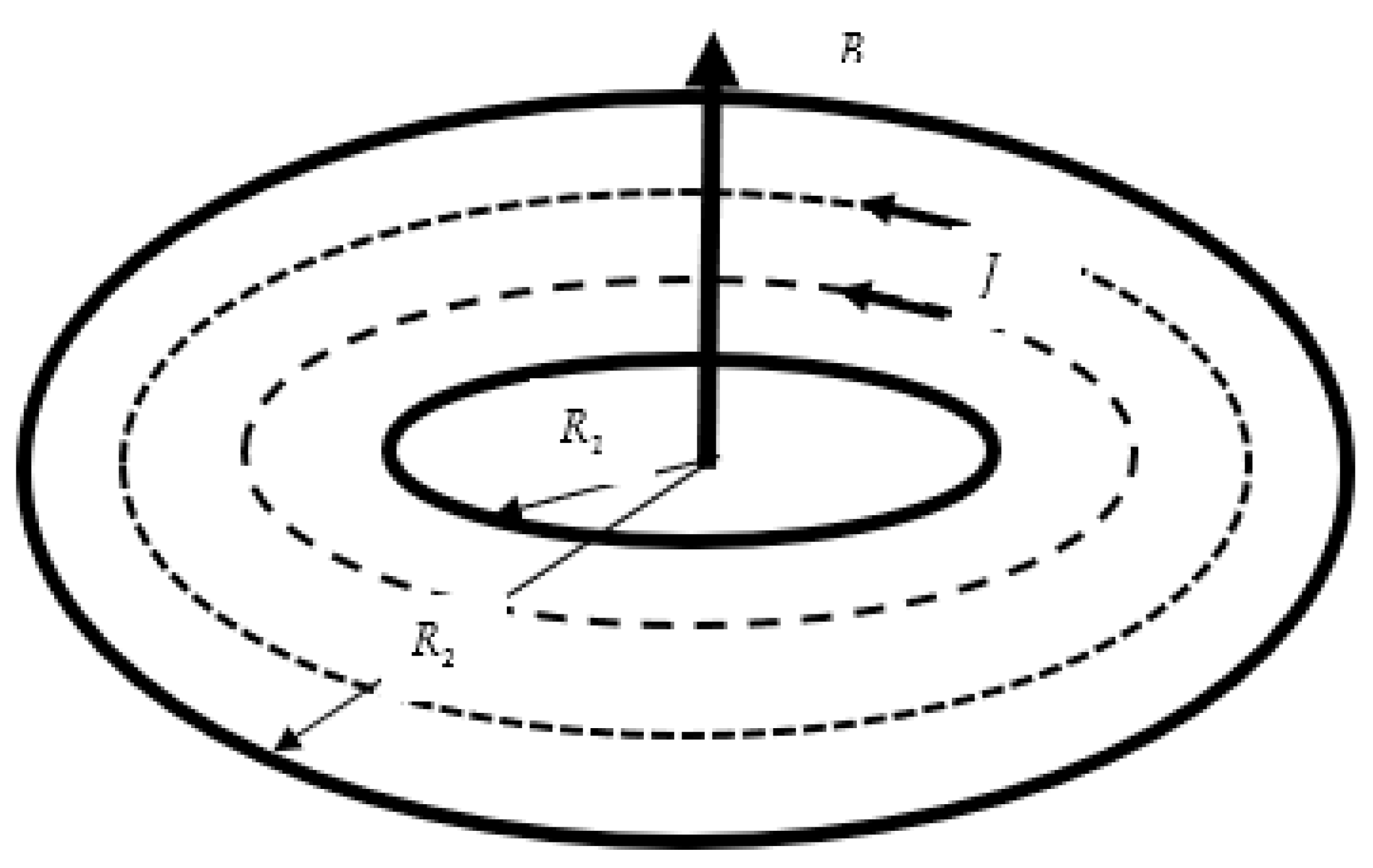
If , , and satisfy the condition (B), then Equation (1) becomes the mutual inductance between two ordinary coplanar disks [10,11]. In Figure 1, the constant azimuthal current is shown for one thin disk coil. Then:
where
- are equally spaced turns of disks,
- are inner radii of disks (in m),
- are outer radii of disks (in m).
The self-inductance of a disk coil with equally spaced turns and as inner and outer radii, respectively, is given by [10]:
This formula can be obtained directly from Equation (2) with
2.2. Concentric Coplanar Bitter Disks
The Bitter coils of the rectangular cross-section are coils, where the azimuthal current densities in the coils conductor are inversely proportional to their radii. The mutual inductance between two concentric Bitter circular coils of the rectangular cross-section is given by [17,18,19]:
where
and are the current densities, which are not constant [13].
The total current through one Bitter coil [13] is:
where is the current density pro-unit area, and is the thickness of the coil.
The value of the total current could be arbitrary. Obviously, the higher this value is, the greater is the value of the magnetic field intensity inside the Bitter plate. However, the upper value of the total current is strongly limited by different factors. The most important factors are the conductive heating of the coil and the stresses in the coil due to the Lorenz pressure of the magnetic field. The analytical approach can only be applied to the coil having cylindrical symmetry, which means that there is no change in geometry when rotating about one axis and when magnetoresistance phenomenon, eddy currents, plastic deformations, and thermal stresses are neglected [13,14].
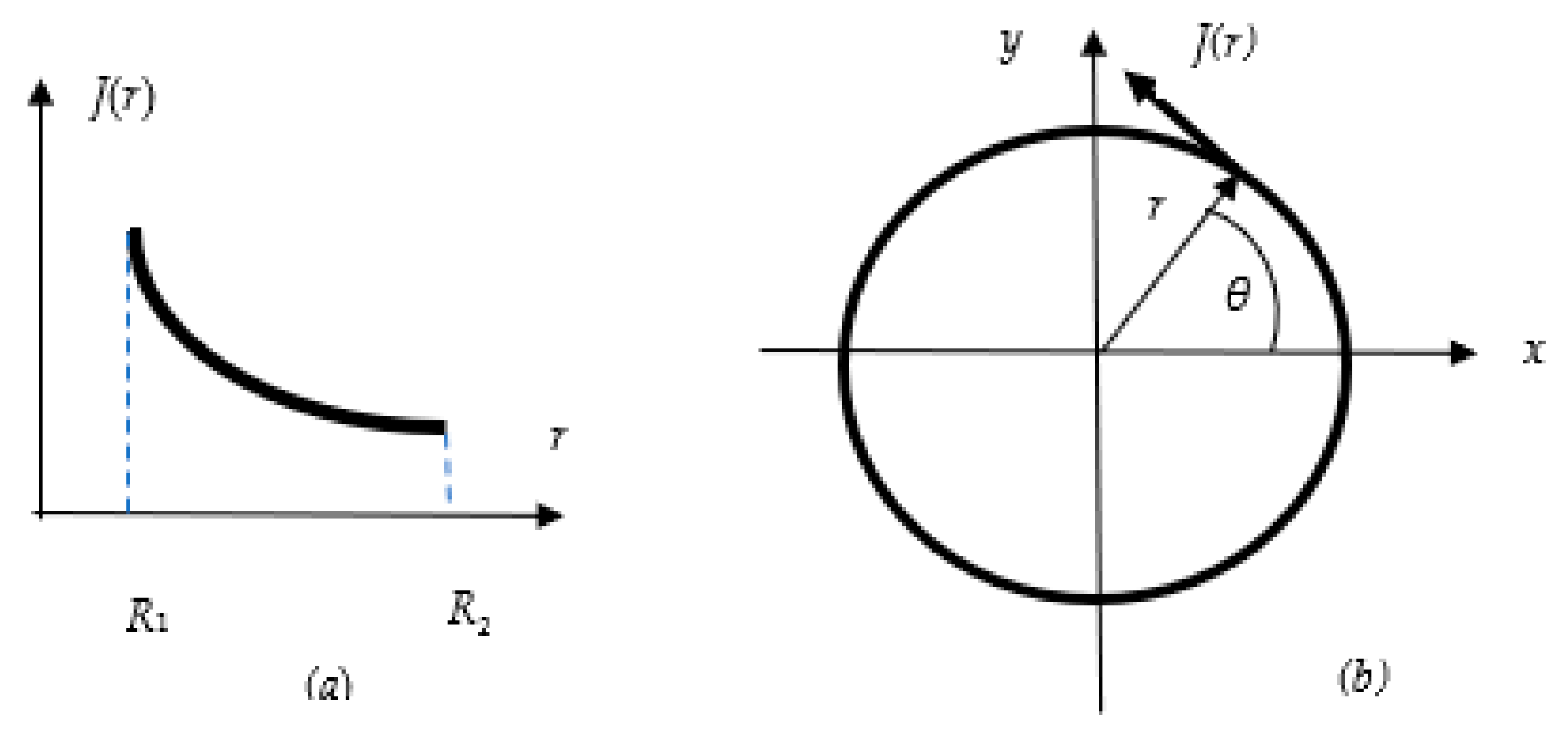
The current density distribution (Figure 2) that guarantees the constant electric potential over all contours with different radii is [13]:
where C is the constant which depends on the thickness function
If the thicknesses of the first and second Bitter coil of the rectangular cross-section are constants from [17,18,19], we obtain the current densities in them:
where
and
- are equally spaced turns of coils,
- are radii (in m) of the first coil with the axial height (in m),
- are radii (in m) of the second coil with the axial height (in m),
- is the non-constant current density in the first coil (in A/m2),
- is the non-constant current density in the second coil (in A/m2),
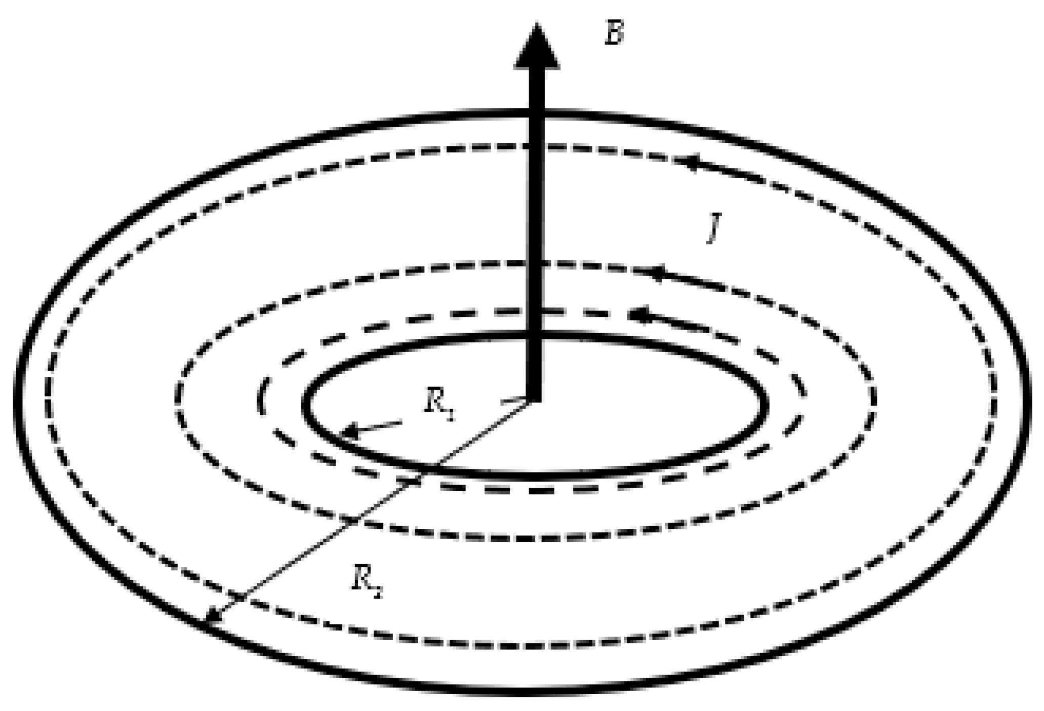
If , , and satisfy the condition (B), Equation (4) becomes the mutual inductance between two coplanar Bitter disks [22]. In Figure 3, the non-uniform azimuthal current is shown for one thin disk coil. Then,
and the self-inductance of the Bitter disk coil is given by [19]:
This formula can be obtained directly from Equation (9), putting .
3. Analytical Calculations
3.1. Ordinary Concentric Coplanar Disks
Before the first integration, let us make the following substitution , so that Equation (2) reads:
Finally, the mutual inductance between two coplanar ordinary disks is:
where
and is the elliptic integral of the second kind [25,26].
The mutual inductance is obtained in a remarkably simple form over the elliptic integral of the second kind and one simple integral whose kernel function is the continuation and integrability over the domain of the integration, so that Equation (6) is applicable in the regular or the singular cases (disks are in the contact or overlap).
For calculating the self-inductance of the ordinary disk coil, one can use Equation (2) or directly put , and into Equation (8), which leads to:
where
and .
We put () and Equation (13) reads:
where
From Equation (13) or Equation (14) it is possible to obtain the self-inductance of the full disk ( and ):
3.2. Concentric Coplanar Bitter Disks
Before the integration, let us make the substitution, so that Equation (9) reads:
Finally, the mutual inductance between two coplanar Bitter disks is:
where
with
The mutual inductance is obtained in an amazingly simple form over the elliptic integral of the second kind. It is applicable in the regular or the singular cases (disks are in contact or overlap).
For calculating the self-inductance of the Bitter disk coil, one can use Equation (10) or directly put , and into Equation (17), which leads to:
where
Thus, either the mutual inductance or the self-inductance for the Bitter disks are obtained in the close form over the elliptic integral of the second kind.
4. Numerical Validation
In this work, all calculations were made in Mathematica programming [27].
Example 1
Calculate the self-inductance of the ordinary real coils with the real thickness d = 0.02 m, and the radii, , and .
Obviously, , and the condition (B) is satisfied, so that the real coil can be practically considered as the concentric coplanar thin disk coil, for which applying Equation (13), the self-inductance is:
The discrepancy between these two calculations is 0.6314%. The results are in particularly good agreement. We conformed the validity of our approach.
Example 2
Calculate the mutual inductance between two ordinary real coils with the real thickness d = 0.001 (m), with the radii , and .
Obviously, for the two real coils can be considered as the two concentric coplanar thin disk coils for which, applying Equation (12),
These results are in excellent agreement.
Example 3
Calculate the self-inductance of the real ordinary coil [9,11] and the self-inductance of the thin disk coil (14). The coil dimensions and the number of turns are as follows:
The self-inductances as the thickness of the real coil is changing are given in Table 1 compared with the earlier calculations [9,11].
Equations (13) or (14) give the self-inductance of the ordinary concentric coplanar thin disk coil (Table 1),
All results are in exceptionally good agreement with the result obtained in the semi-analytical form (14). Thus, the ordinary real coils with the thicknesses which are remarkably smaller than their radii can be considered as the thin concentric coplanar disk coils. Again, our assumption is proven.
Example 4
Example 5
Table 3 shows calculations of the self-inductance of the ordinary disk for various shape factors and for values remarkably close to the logarithmic singularity as . These calculations are compared to two sets of the results obtained by the Spielrein method, see Ref. [5] and Equation (58) in Ref. [12].
Example 6
In this example, we show the performance of the Equation (8) when the singularity is approached (). We compare the results of Equation (14) with those obtained by the asymptotic Equations (12) and (58) of Ref. [12], see Table 4.
All the results are in a remarkably good agreement. This shows that Equation (14) has a large range of applications.
Example 7
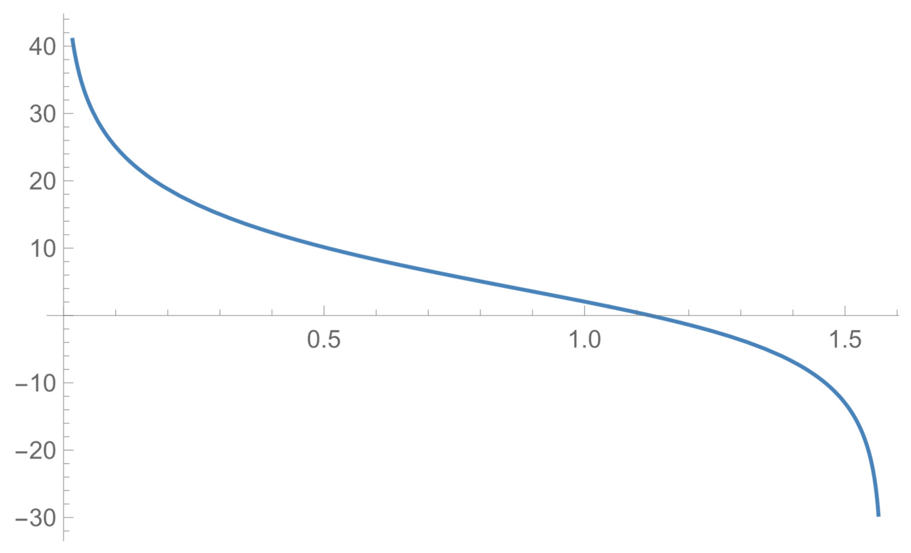
Let us provide the graphical presentation of the kernel function of the integral which appears in Equations (13) and (14), for which .
The kernel function is given by:
and is displayed in Figure 4 in the interval . From Figure 4 one can conclude about two discontinuities of the type II because does not exist at , .
Using the numerical integration in MATLAB programming, we obtain:
Using the numerical integration in Mathematica programming, we obtain:
Both numerical integrations are in very good agreement.
Example 8
Here, we calculate the self-inductance of the full disk coil, for which and .
From Equation (15), the self-inductance of the full disk is:
To verify this result, we use Equation (14), and for that gives:
We obtain the identical result.
Example 9
Example 10
We calculate the mutual inductance between two disk coils for which , and .
Obviously, the disks completely overlap, and it is a case of self-inductance. Let us apply Equation (12) for the mutual inductance of the disk coils. It gives:
Applying Equation (13) for the self-inductance of the disk coil, we obtain:
We obtain the identical result.
Thus, we show that simple Equation (13) is general for any case, either for the regular or for the singular. This is also confirmed in the previous examples.
Example 11
Here, we calculate the self-inductance of the real Bitter coil with the real thickness b = 0.02 m, the radii , and .
Obviously, as , then condition (B) is satisfied, so that the real Bitter coil can be practically considered as the thin Bitter disk coil, for which applying Equation (18), the self-inductance is:
The discrepancy between these two calculations is 0.8242%. The results are in a very good agreement. This confirms the validity of our approach.
Example 12
Here, we calculate the mutual inductance of the two real Bitter coils with the real thickness d = 0.001 m, the radii , and .
For these two real Bitter coils [17], the mutual inductance is:
By finite-element method (FEM), the mutual inductance is:
Thus, the results obtained by three different methods are in excellent agreement.
Obviously, two real Bitter coils can be practically considered as the two thin Bitter disk coils because the condition (B) is satisfied.
Applying Equation (17), the mutual inductance is:
We see that the obtained result is in an excellent agreement with the earlier ones.
Example 13
The mutual inductance for two Bitter disk coils is given in Table 6, where the radii are given as ,, and , and varying between 1 and 9 m. The number of turns for the disk is 1000. This covers all the overlap cases.
From Table 6, we can observe very good agreement of all results. There is negligible discrepancy between the presented results because the filament method [18,19] is approximative and depends on the number of divisions of the disk coils. Note that the more disk divisions are more computing time is needed.
Example 14
In this example, the self-inductance of the Bitter coil are calculated for the thickness b = 0.001, with the radii , and . Calculating the self inductance of this coil.
By FEM, the self-inductance is:
Equation (17) gives the mutual inductance between two Bitter disk coils. Let us take ,. Applying Equation (17), we obtain:
Applying Equation (18) for the self-inductance of the Bitter coil, we have:
We showed that all results for the self-inductance, obtained by the different methods, are in particularly good agreement.
Example 15
In Table 7, the self-inductance of the real Bitter coil [23,24] are given with the coil dimensions and the number of turns N = 100, for widely changing thickness of the real coils.
The Equation (18) for the thin Bitter disk coil gives the self-inductance:
All results [23,24] are in a very good agreement with the result obtained in the analytical form (18). Thus, the real Bitter coils with thicknesses which are remarkably smaller than their radii can be considered as the concentric coplanar thin Bitter coils.
From the previous examples, we proved that it is possible to treat the real circular coils of the rectangular cross-section, whose thicknesses are remarkably smaller than their radii (conditions (A) and (B)), as the thin disk coils (pancakes). In these cases, we use the amazingly easier analytical and semi-analytical expressions. It validates our presented method.
5. Conclusions
In this paper, we presented remarkably simple formulas for calculating the self- and mutual inductance of ordinary concentric coplanar disk coils with azimuthal current density and concentric coplanar Bitter disk coils with non-uniform current density. All presented formulas were obtained under some valuable conditions for the real coils of the rectangular cross-section, either for ordinary real coils or the real Bitter coils. For the concentric coplanar ordinary disks, the formulas were obtained in the semi-analytical form as the combination of the elliptic integral of the second kind and a simple integral. For the concentric coplanar thin Bitter disks, the formulas were obtained in the analytical form as the elliptical integral of the second kind. All cases of either the regular or the singular (disks overlap) were covered with obtained formulas. Many examples presented are shown to approve the correctness of the presented method. The presented formulas are simple to use for potential readers which are not familiar with complicated special functions, such as Bessel functions, generalized hypergeometric functions, or Mellin transform.
Funding
This research received no external funding.
Informed Consent Statement
Informed consent was obtained from all subjects involved in the study.
Acknowledgments
The authors thank Y. Ren of the Hefei Institute of Plasma Physics, Chinese Academy of Science, Anhui for providing extremely high precision calculations for the mutual and self-inductance of the Bitter disk coil which has proven invaluable in validating the methods presented here.
Conflicts of Interest
The author declares no conflict of interest.
References
- Grover, F.W. Inductance Calculations; Dover: New York, NY, USA, 1964. [Google Scholar]
- Dwight, H.B. Electrical Coils and Conductors; McGraw-Hill Book Company, Inc.: New York, NY, USA, 1945. [Google Scholar]
- Snow, C. Formulas for Computing Capacitance, and Inductance; National Bureau of Standards: Washington, DC, USA, 1954. [Google Scholar]
- Kalantarov, P.L.; Tseytlin, L.A. Inductance Calculations; National Power Press: Moscow, Russia, 1955. (in Russian) [Google Scholar]
- Spielrein, J. Die Induktivität eisenfreier Kreisringspulen. Arch. Elektrotechnik 1915, 3, 187–202. [Google Scholar] [CrossRef]
- Butterworth, S. On the self-inductance of single-layer flat coils. Proc. Phys. Soc. London 1919, 32, 31–37. [Google Scholar] [CrossRef] [Green Version]
- Rosa, E.B.; Grover, F.W. Scientific Papers of the National Bureau of Standards, 3rd ed.; National Bureau of Standards: Washington, DC, USA, 1948. [Google Scholar]
- Wang, Y.; Xie, X.; Zhou, Y.; Huan, W. Calculation and modeling analysis of mutual inductance between coreless circular coils with rectangular cross section in arbitrary spatial position. In Proceedings of the 2020 IEEE 5th Information Technology and Mechatronics Engineering Conference (ITOEC), Chongqing, China, 12–14 June 2020. [Google Scholar] [CrossRef]
- Luo, Y.; Chen, B. Improvement of self-inductance calculations for circular coils of rectangular cross section. IEEE Trans. Mag. 2013, 49, 1249–1255. [Google Scholar] [CrossRef]
- Župan, T.; Štih, Ž.; Trkulja, B. Fast and precise method for inductance calculation of coaxial circular coils with rectangular cross section using the one-dimensional integration of elementary functions applicable to super conducting magnets. IEEE Trans. Appl. Supercond. 2014, 24, 4901309. [Google Scholar] [CrossRef]
- Doležel, I. Self-inductance of an air cylindrical coil. Acta Tech. CSAV 1989, 34, 443–473. Available online: http://www.digitalniknihovna.cz/knav/view/uuid:1f604d8b-e630-4bc7-8173-88846837782f (accessed on 25 April 2021).
- Conway, J.T. Analytical solutions for the self- and mutual inductances of concentric coplanar disk coils. IEEE Trans. Magn. 2013, 49, 1135–1142. [Google Scholar] [CrossRef]
- Babic, S.I.; Akyel, C. An improvement in the calculation of the self-inductance of thin disk coils with air-core. WSEAS Trans. Circuits Syst. 2004, 3, 1621–1626. [Google Scholar]
- Bitter, F. The design of powerful electromagnets Part II. The magnetizing coil. Rev. Sci. Instrum. 1936, 7, 482–489. [Google Scholar] [CrossRef]
- Kobilev, V. Optimal bitter coil solenoid. arXiv 2016, arXiv:1610.06607v2. [Google Scholar]
- Zaitov, O.; Koluhuzin, V.A. Bitter coil design methodology for electromagnetic pulse metal processing techniques. J. Manuf. Process. 2014, 16, 551–562. [Google Scholar] [CrossRef]
- Yu, Y.; Luo, Y. Inductance calculations for non-coaxial Bitter coils with rectangular cross-section using inverse Mellin transform. IET Electr. Power Appl. 2019, 13, 119–125. [Google Scholar] [CrossRef]
- Ren, Y.; Wang, F.; Kuang, G.; Chen, W.; Tan, Y.; Zhu, J.; He, P. Mutual inductance and force calculations between coaxial bitter coils and superconducting coils with rectangular cross section. J. Supercond. Nov. Magn. 2011, 24, 1687–1691. [Google Scholar] [CrossRef]
- Ren, Y.; Kuang, G.; Chen, W. Inductance of bitter coil with rectangular cross-section. J. Supercond. Nov. Magn. 2013, 26, 2159–2163. [Google Scholar] [CrossRef]
- Conway, J.T. Non coaxial force and inductance calculations for bitter coils and coils with uniform radial current distributions. In Proceedings of the 2011 International Conference on Applied Superconductivity and Electromagnetic Devices, Sydney, NSW, Australia, 14–16 December 2011; pp. 61–64. [Google Scholar]
- Chen, J.W. Modeling and decoupling control of a linear permanent magnet actuator considering fringing effect for precision engineering. IEEE Trans. Magnet. 2021, 57, 8104115. [Google Scholar] [CrossRef]
- Babic, S.I.; Akyel, C. Mutual inductance and magnetic force calculations for coaxial Bitter disk coils (Pancakes). IET Sci. Meas. Technol. 2016, 10, 972–976. [Google Scholar] [CrossRef]
- Babic, S.; Akyel, C. Self-inductance of the circular coils of the rectangular cross-section with the radial and azimuthal current densities. Physics 2020, 2, 352–367. [Google Scholar] [CrossRef]
- Babic, S.; Akyel, C. Addendum: Self-inductance of the circular coils of the rectangular cross-section with the radial and azimuthal current densities. Physics 2021, 3, 1. [Google Scholar] [CrossRef]
- Gradshteyn, I.S.; Ryzhik, I.M. Table of Integrals, Series and Products, 7th ed.; Academic Press: New York, NY, USA, 2007. [Google Scholar]
- Prudnikov, A.P.; Brychkov, A.; Marichev, O.I. Integrals and Series; Gordon and Breach: New York, NY, USA, 1990; Volume 3. [Google Scholar]
- Wolfram, S. The Mathematica Book, 5th ed.; Wolfram Media: Champaign, IL, USA, 2003. [Google Scholar]
Figure 1.
Thin disk coil carrying the constant azimuthal current density, J.

Figure 2.
(a) The non-constant current density in the Bitter coil. (b) Dependence of the azimuthal current density of the angle θ.
Figure 2.
(a) The non-constant current density in the Bitter coil. (b) Dependence of the azimuthal current density of the angle θ.

Figure 3.
Thin disk Bitter coil carrying the azimuthal current density J and which has a variation according to the radius , which is different.
Figure 3.
Thin disk Bitter coil carrying the azimuthal current density J and which has a variation according to the radius , which is different.

Figure 4.
in the interval


Table 1.
The self-inductance when is extremely decrasing.
| [9,11] | ||
|---|---|---|
| 10−3 | 53592975459863 | |
| 10−4 | 8 | 3592975459863 |
| 10−5 | 592975459863 | |
| 10−6 | 92975459863 | |
| 10−7 | 2975459863 | |
| 10−8 | 975459863 | |
| 10−9 | 936402 | 75459863 |
| 10−10 | 5459863 | |
| 10−11 | 459863 | |
| 10−12 | 59863 |
Table 2.
Self-inductance given as in μH/m.
| α | [4] | [12], Equation (58) | Equation (14), This Work |
|---|---|---|---|
| 1.5 | 3.9375 | ||
| 3 | 4.1202 | ||
| 4 | 4.6535 | ||
| 7 | 6.5440 | ||
| 9 | 7.8795 | ||
| 19 | 14.740 | ||
| 39 | 28.628 |
Table 3.
Comparison of calculations for the self-inductance (in µH/m) for values of the shape factor, both close to and far from the singularity .
Table 3.
Comparison of calculations for the self-inductance (in µH/m) for values of the shape factor, both close to and far from the singularity .
| α | [5] | [12], Equation (58) | Equation (14), This Work |
|---|---|---|---|
| 50 | |||
| 10 | |||
| 3 | |||
| 1.5 | |||
| 1.1 | |||
| 1.01 | |||
| 1.001 | |||
| 1.00001 | |||
| 1.000001 | |||
| 1.0000001 |
Table 4.
Comparison of the results of Equation (14) with those from [12] (Equaition (58) and the asymptotic formula (20) there) as the singularity at the unit shape factor is approached. The results are given in μH/m.
Table 4.
Comparison of the results of Equation (14) with those from [12] (Equaition (58) and the asymptotic formula (20) there) as the singularity at the unit shape factor is approached. The results are given in μH/m.
| [12], Equation (58) | [12], Equation (20) | Equation (14), This Work | |
|---|---|---|---|
| 10−1 | 4.998068846886786 | ||
| 10−2 | |||
| 10−3 | |||
| 10−6 | |||
| 10−8 | |||
| 10−10 | |||
| 10−12 | |||
| 10−15 | |||
| 10−16 |
Table 5.
Mutual inductance for all overlap cases.
| [12] | ||
|---|---|---|
| 0.1 | ||
| 0.2 | ||
| 0.3 | ||
| 0.4 | ||
| 0.5 | ||
| 0.6 | ||
| 0.7 | ||
| 0.8 | ||
| 0.9 |
Table 6.
Mutual inductance for all overlap cases.
| [18,19] | ||
|---|---|---|
| 1 | 6.176890611593179 | |
| 2 | 8.441929573292805 | |
| 3 | 10.32810057022684 | |
| 4 | 11.44063208654759 | |
| 5 | 10.40633203780527 | |
| 6 | 8.263044761562908 | |
| 7 | 7.051548623257631 | |
| 8 | 6.338568878810852 | |
| 9 | 5.832749077642109 |
Table 7.
The self-inductance for the real Bitter coil and the thin Bitter disk coil with strongly varying thickness.
Publisher’s Note: MDPI stays neutral with regard to jurisdictional claims in published maps and institutional affiliations. |
© 2021 by the author. Licensee MDPI, Basel, Switzerland. This article is an open access article distributed under the terms and conditions of the Creative Commons Attribution (CC BY) license (https://creativecommons.org/licenses/by/4.0/).
Share and Cite
MDPI and ACS Style
Babic, S. Analytical and Semi-Analytical Formulas for the Self and Mutual Inductances of Concentric Coplanar Ordinary and Bitter Disk Coils. Physics 2021, 3, 240-254. https://0-doi-org.brum.beds.ac.uk/10.3390/physics3020018
AMA Style
Babic S. Analytical and Semi-Analytical Formulas for the Self and Mutual Inductances of Concentric Coplanar Ordinary and Bitter Disk Coils. Physics. 2021; 3(2):240-254. https://0-doi-org.brum.beds.ac.uk/10.3390/physics3020018
Chicago/Turabian StyleBabic, Slobodan. 2021. "Analytical and Semi-Analytical Formulas for the Self and Mutual Inductances of Concentric Coplanar Ordinary and Bitter Disk Coils" Physics 3, no. 2: 240-254. https://0-doi-org.brum.beds.ac.uk/10.3390/physics3020018