Determining Pitch-Angle Diffusion Coefficients for Electrons in Whistler Turbulence


1
Institut für Theoretische Astrophysik, Universität Heidelberg, Albert-Ueberle-Strasse 2, 69120 Heidelberg, Germany
2
Centre for Space Research, Northwest-University, Potchefstroom 2520, South Africa
3
Max-Planck-Institute for Solar System Research, Justus-von-Liebig-Weg 3, 37077 Göttingen, Germany
4
Institut für Theoretische Physik IV, Ruhr-Universität Bochum, Universitätsstrasse 150, 44801 Bochum, Germany
5
Institut für Theoretische Physik und Astrophysik, Christian-Albrechts-Universität zu Kiel, Leibnizstr. 15, 24118 Kiel, Germany
*
Author to whom correspondence should be addressed.
Physics 2022, 4(1), 80-103; https://0-doi-org.brum.beds.ac.uk/10.3390/physics4010008
Submission received: 30 August 2021
/
Revised: 30 November 2021
/
Accepted: 7 December 2021
/
Published: 20 January 2022
(This article belongs to the Special Issue A Themed Issue in Honor of Professor Reinhard Schlickeiser on the Occasion of His 70th Birthday)
Abstract
:Transport of energetic electrons in the heliosphere is governed by resonant interaction with plasma waves, for electrons with sub-GeV kinetic energies specifically with dispersive modes in the whistler regime. In this paper, particle-in-cell simulations of kinetic turbulence with test-particle electrons are performed. The pitch-angle diffusion coefficients of these test particles are analyzed and compared to an analytical model for left-handed and right-handed polarized wave modes.
1. Introduction
The solar wind and most phases of the interstellar medium are strongly turbulent media with high magnetic Reynolds numbers of [1]. Turbulence manifests itself in a spectrum of plasma waves at various length scales and frequencies. The energy distribution as a function of the frequency follows a characteristic power law. The current understanding of the turbulent processes is such that energy is injected at large scales, i.e., at small wave numbers and frequencies, and then cascades to smaller spatial scales.
The energy spectrum can be divided into several regimes, each may span several orders of magnitude in wave number or frequency. At the largest scales, the injection range is found, which then transitions into the inertial range. The inertial range can be described by magnetohydrodynamic (MHD) theory, and turbulence is dominated by the interaction of Alfvén waves. At smaller scales, kinetic effects of the particles come into play.
This high wave number regime is often referred to as the kinetic, dispersive, or dissipation range of the spectrum, since the waves become dispersive and dissipation starts to set in. While the spectrum extends to even smaller scales, damping eventually becomes dominant and leads to an exponential cutoff of the energy spectrum.
Power-law distributions of the fluctuating magnetic energy are expected in the injection, inertial, and dissipation range of the spectrum. However, the spectral indices may differ among the individual regimes. Goldreich and Sridhar [2,3] presented a detailed model of the turbulent energy cascade in the inertial regime. Their model predicts a spectral index of , which actually seems to be realized in the solar wind [4]. Subsequent models by Galtier et al. [5,6] give rise to a spectral index .
Kinetic turbulence in the dissipation range is an active field of research [7]. In particular, the composition of the wave spectrum is subject to discussion, because a transition from non-dispersive Alfvén waves to dispersive wave modes is expected. Possible candidates for the waves in the dissipation range are the so-called kinetic Alfvén waves (KAWs) and whistler waves [8].
The impact of kinetic turbulence on the transport of energetic particles is another major topic. The transport of energetic protons is well described by models of Alfvénic turbulence, since the protons mainly interact with these waves at low frequencies. The theoretical framework of quasi-linear theory (QLT) can be used to describe particle transport by a series of resonant interactions with the magnetic fields of Alfvén waves, which leads to scattering of the particles [9,10,11]. This theory describes changes of the particles’ pitch angles (the angle of the velocity vector relative to a background magnetic field), momenta, or positions as diffusion processes and allows to predict diffusion coefficients and other quantities, such as the mean free path, which can be compared to observations.
Dispersive waves are more difficult to handle in (analytical) theory. Nonetheless, QLT can also yield predictions for particle transport in a medium containing dispersive waves [12,13]. The introduction of dispersive waves can even solve some of the problems that are encountered if a purely Alfvénic spectrum of waves is assumed [14]. Still, the model remains an approximation, and computer simulations are used to clarify some of the details that are not included in the analytical theory. Different kinds of simulations are used to study different physical regimes and processes—from the acceleration of particles [15,16] to the transport of energetic particles—considering both non-dispersive [17] and dispersive waves [18,19].
The key problem that has been chosen for the subject of this study is the process of electron transport in dispersive turbulence. The transport of electrons at sub-GeV energies has been of high interest for quite some time [20]. As mentioned above, particle acceleration in Alfvénic turbulence in the inertial range is well understood. However, turbulence on kinetic scales still poses problems for both observations and modeling.
2. Theory
2.1. Turbulence Theory
From the observations, it is not entirely clear which types of plasma waves constitute the spectrum of turbulent waves in the dispersive and dissipative regime. KAWs and whistler waves are both possible candidates [8]. While KAWs represent the continuation of the Alfvén mode (Equation (13) below) in the dispersive regime with very large perpendicular wave numbers (perpendicular wavelength in the range of proton gyroradius), whistler waves (Equation (16) below) are right-handed polarized modes at large wave numbers. It is reasonable to assume that non-dispersive Alfvén waves simply transition to KAWs. However, observations reveal that whistler waves are also present in various regions of the heliosphere, such as in the interplanetary medium [21], close to interplanetary shocks [22,23] or planetary bow shocks [24], and also in the Earth’s ionosphere and foreshock region [25,26].
Whereas left-handed polarized Alfvén waves are damped by protons and cannot cascade to frequencies above the proton cyclotron frequency, a spectrum of whistler waves may extend to frequencies beyond the ion-cyclotron frequencies. Whistler waves primarily interact with electrons and are also damped by electrons at higher frequencies (close to the electron cyclotron frequency). This is an interesting aspect of kinetic turbulence, since a population of whistler waves can heat the electrons in the solar wind or even accelerate particles in the high-energy tail of the thermal spectrum.
Kinetic turbulence includes the smallest length scales, where the interaction of waves and particles becomes important. Although the wave-particle interactions are not explicitly included in the theory, their effect has to be considered by allowing dispersive waves and damping. This regime is generally more complicated and less understood than MHD turbulence.
The general picture associated with turbulence is as follows. Energy is injected into the system at a large outer scale, small wave numbers k. The energy is transported via the interaction of waves to smaller spatial scales (larger wave numbers), and the (magnetic) energy spectrum, , follows a power-law distribution. This is the inertial range. The spectrum steepens as the kinetic regime or dissipation range is reached, but energy is still transported to smaller scales. First, only ion effects will start influencing the plasma dynamics, but at even larger wave numbers, the electrons can also interact with the plasma waves. This is where the energy spectrum is cut off. One aspect that has been discussed in greater detail since the seminal paper of Goldreich and Sridhar [3] is the possible anisotropy with respect to the background magnetic field: the turbulent spectrum may behave differently depending on wave numbers parallel () or perpendicular () to the background magnetic field.
The special case of whistler turbulence has been discussed in greater detail. The properties of this whistler turbulence have been analyzed using kinetic simulations in two [27,28] and three [29,30,31,32] dimensions. These studies suggest a steeper energy spectrum than for Alfvénic turbulence, with a spectral index s in the range between and and a possible break in the energy spectrum [32]. Results by Chang [30] also suggest that the wave vector anisotropy depends on the choice of the plasma beta. A relatively isotropic spectrum is obtained for a plasma beta , whereas yields an anisotropic cascade which favors the transport of energy to larger . The plasma beta is the ratio of thermal to magnetic energy. The anisotropy additionally depends on the energy deployed to the electromagnetic fields of the turbulent whistler waves [29].
2.2. Subluminal Parallel Waves in Cold Plasmas
In warm thermal plasmas with low plasma betas, the real part of the dispersion relation agrees well with the cold plasma dispersion relation, so, the latter is used here. In addition, the resonance broadening effects, caused by a finite imaginary part of the dispersion relation in warm plasmas implying a finite weak-damping rate; those effects were considered by Schlickeiser and Achatz [33].
Using the convention of frequencies , where is the real part of the generally complex frequency, but (here, the case , also known as slab case, is treated), the dispersion relation of right-handed (“R”) and left-handed (“L”) polarized undamped low-frequency (, with being the electron gyrofrequency) parallel Alfvén wave in a cold electron-proton background plasma reads [34]:
with the proton-to-electron mass ratio, , and the Alfvén speed, Here, is the ion plasma frequency, is the electron plasma frequency, is the ion gyrofrequency, is the electron gyrofrequency, B is the magnetic field, is the plasma beta, and c is the speed of light. For subluminal wave phase speeds,
which has to be checked a posteriori, the dispersion relation (4) simplifies to
It is convenient to introduce dimensionless frequencies and parallel wave numbers by defining
respectively, with
so that the subluminal dispersion relation becomes
with the two solutions,
As is always positive, the solution describes forward-moving waves with positive phase speed, whereas the negative solution describes backward-moving waves.
2.2.1. Left-Handed Modes
2.2.2. Right-Handed Modes
Depending on k, different regimes can be identified:
The first range describes the linear dispersion regime, the second range is the whistler regime, and the last range is the electron–cyclotron range. While these approximate solutions provide good estimates to the real solution, there is a major problem: the solutions do not provide continuous coverage. An alternative approximation is
In the following, the particle scattering by parallel waves at electron or ion cyclotron frequencies are ignored as soon as these are highly damped in a realistic warm thermal plasma, so that the resonant interaction does not apply; see [33] for a discussion of wave-particle interactions with damped waves. For left-handed and right-handed polarized waves, this restricts the normalized wave numbers to values of and , respectively.
2.3. Particle Transport
Any charged particle of given velocity v, Lorentz factor , pitch-angle cosine , mass m, charge with , being the ion charge number, and relativistic gyrofrequency with positive with being the particle’s non-relativistic gyrofrequency, q being the electric charge, and being the magnetic background field, interacts with parallel right-handed and left-handed polarized plasma waves whose wave number, k, and real frequency, , obey the resonance condition,
Introducing
with the particle momentum p and the dimensionless frequency and wave number (7), the resonance condition (18) reads:
with
The quasilinear Fokker–Planck coefficient for the pitch-angle cosine, , is given by
with the magnetic fluctuation spectra of right/left-handed polarized waves , where the total magnetic field fluctuations are determined as in [35]:
In Equation (22), the frequencies are determined by the solutions of the dispersion relations, discussed in Section 2.2 above. The function is the Dirac delta function.
In terms of the normalized wave number, , and frequency, , the Fokker–Planck coefficient (22) reads:
The calculation of the Fokker–Planck coefficient requires a knowledge of the magnetic fluctuation spectra. The correct theoretical description is complicated, as described in Section 2.1 above, but results from numerical calculations can be inferred.
Deriving the Fokker–Planck coefficients in general is quite an involved task but one can derive some limiting cases. It is helpful to account for the relative abundance of forward-moving and backward-moving waves and the corresponding polarization states. Let us introduce the cross helicities, for left/right-handed polarized waves to express the spectra (23) of backward-propagating (“b”) and forward-propagating (“f”) waves:
The step function appears because backward-moving and forward-moving waves only occur at negative and positive wave numbers, respectively. In general, these cross helicities can depend on the wave number, but throughout this article isospectral turbulence is adopted, where are constants (independent of k). The magnetic helicity characterizes the relative abundances of left-handed and right-handed polarized waves:
where is the total wave abundance at a specific wave number. For parallel plasma waves, as soon as no left-handed polarized waves exist at these normalized frequencies.
Using the helicities introduced, the Fokker–Planck coefficient (24) reads:
2.3.1. Interactions in the Whistler Regime
For frequencies above the ion cyclotron frequency, only right-handed waves exist obeying the dispersive whistler mode dispersion relation. As discussed above, the turbulent spectrum typically has a much softer spectral index than 2 (theoretical values are in the range of 3 to 6 [7,36]) in this case.
We consider the case and , only backward-moving right-handed polarized waves, which reduces the Fokker–Planck coefficient (29) to
The result for forward-moving waves is similar:
It can be shown that this equation for protons and electrons has only one solution . In the Alfvénic wave number range (), this is trivial: , which can be positive depending on the signs of and .
In the whistler wave number range (), the proof is a bit more involved. Here, Equation (32) has two solutions:
To obtain real-valued solutions (33) and (34), the condition must be fulfilled. Assuming that this is fulfilled, one notes that for non-negative values of , the solution is always negative, leaving only one solution for . Alternatively, for negative values of the solutions (33) and (34) become
To further evaluate the solution, it is necessary to distinguish between positive (for protons) and negative values (for electrons) of . For electrons the solution is again always negative. For protons, both solutions (35) and (36) are positive, but the second one is
always (for protons ). This solution is positive but is in contradiction with the above-made assumption of the modes in the whistler regime with . This leaves us with only one solution for the resonant wave number in the whistler wave number range.
One then obtains:
The case of forward-moving right-handed polarized waves is similar to the backward-moving ones. The main difference is the resonant wave number,
2.3.2. Alfvén and Whistler Contributions
The total Fokker–Planck coefficient can be written as a sum of Alfvén and whistler contributions:
For the Alfvén wave Fokker–Planck coefficient, inserting the asymptotic expansions of Equations (12) and (15) one obtains:
The whistler contribution is calculated above, while for completeness is given here in the same form:
2.3.3. Electrons
The Fokker–Planck coefficient derived in the previous section hold for any particle. In general, the integration is not complicated as the delta function of the resonance condition helps to simplify the calculations. However, a specific turbulent spectrum has to be defined. We refrain from performing the integral here but point out which interaction will take place. There is a clear difference between electrons and protons, and the discussion in this Section is limited to the electron case.
For Alfvén waves, one can distinguish the interaction of electrons with forward/backward-moving left/right-handed modes. Defining
one can constrain the waves for which the resonant interaction with electrons is possible:
- (1)
- backward-moving right-handed polarized Alfvén waves for all pitch-angle cosines with and ;
- (2)
- backward-moving left-handed polarized Alfvén waves for all pitch-angle cosines with ; and
- (3)
- forward-moving right-handed polarized Alfvén waves for all pitch-angle cosines with and ;
- (4)
- forward-moving left-handed polarized Alfvén waves for all pitch-angle cosines with and .
For whistler waves, additionally
is defined. The resonant interaction takes place within the following range:
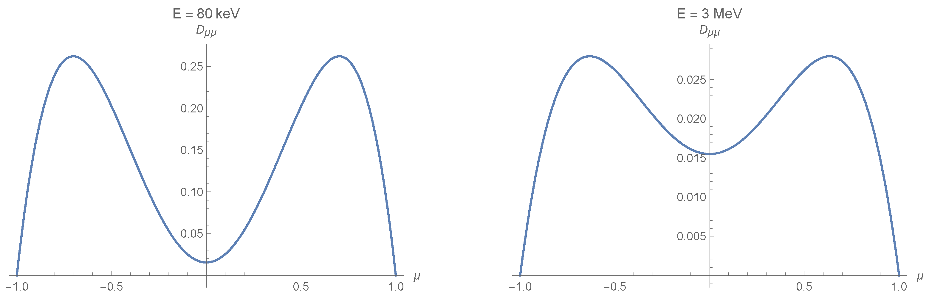
The resulting total Fokker–Planck scattering coefficient is shown in Figure 1.
3. Numerical Methods
3.1. Particle-in-Cell Simulations
To be able to model dispersive waves of different kinds and to obtain a self-consistent description of electromagnetic fields and charged particles in the plasma, a fully kinetic particle-in-cell (PiC) approach [37] is employed here. In particular, the explicit second-order PiC code ACRONYM [38] is used which is fully relativistic, parallelized and three-dimensional. Although the PiC method might not be the most efficient numerical technique when dealing with proton effects, we still favor this approach because of its versatility. A more detailed discussion of advantages and drawbacks as well as a direct comparison of PiC and MHD approaches with the specific problem of the interaction of protons and left-handed polarized waves can be found in Sections 3 and 6 of Ref. [39]. However, the PiC approach is well-suited for the study of electron scattering as soon as the time and length scales of electron interactions are closer to the scales of time step lengths and cell sizes in PiC simulations, thus reducing computing time compared to simulations, in which proton interactions are studied.
The details of the PiC code are not discussed here. The simulation technique used here does not differ from standard techniques. Two points, however, to be mentioned: the initialization of turbulence and the tracking of test particles. Turbulence is discussed in Section 3.1.1 just below, because the numerical treatment is inherently connected to the physical processes of turbulence. The treatment of energetic particles is divided into to two parts: the injection of particles and the analysis of the particle data.
3.1.1. Setup of Turbulence Simulations
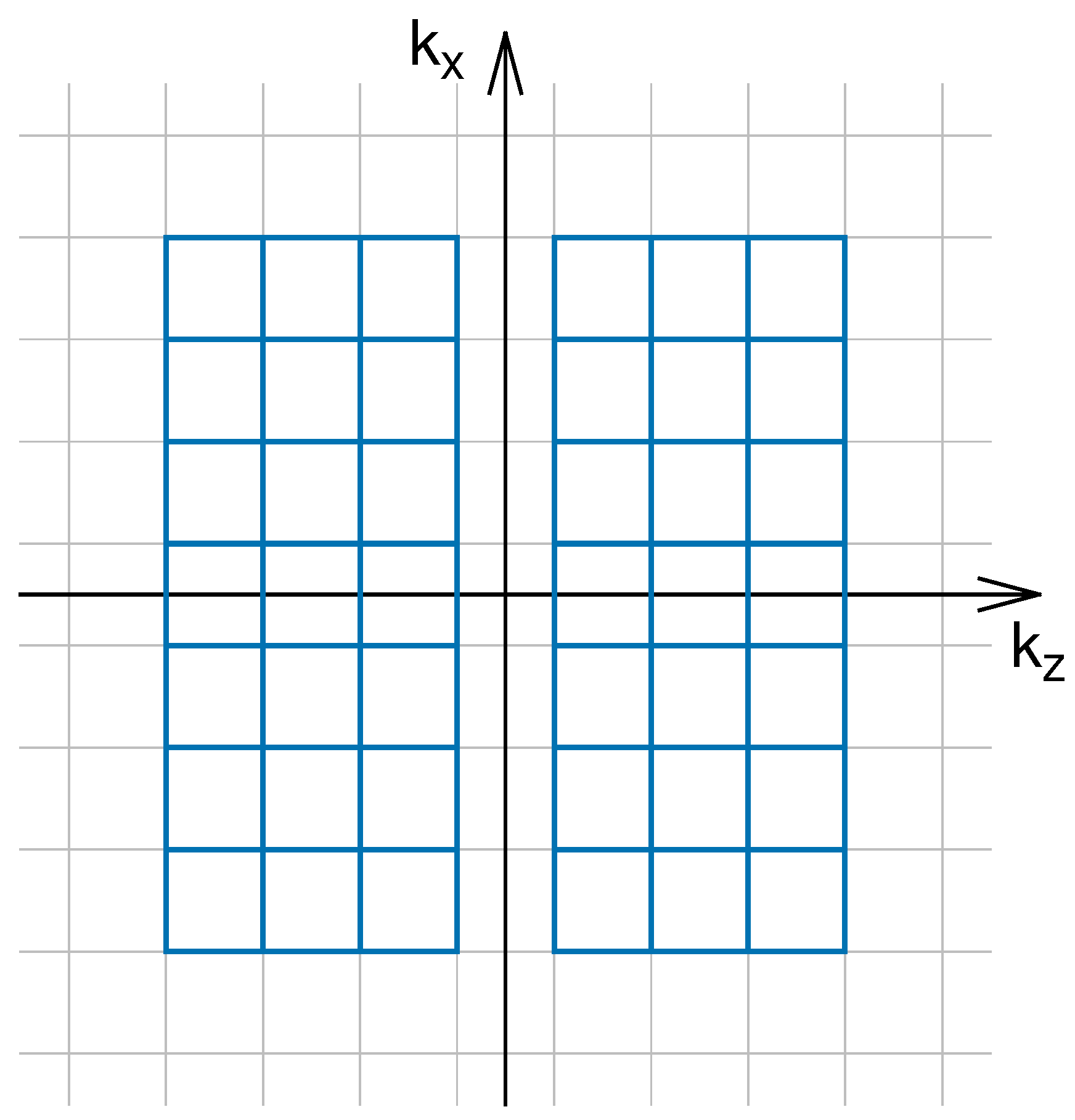
Here, a simulation setup that was inspired by Gary et al. [27] is used. Waves are initialized at low k, . The layout of the initial waves in the wave number space is explained below and is drawn in Figure 2 for the two-dimensional setup. However, in the PiC simulation, the velocity space and the electromagnetic fields are considered three-dimensional. As shown below, the two-dimensional simulations give an energy cascade similar to that of the three-dimensional simulations. As highlighted by Gary et al. [29], the three-dimensional case differs mainly in the anisotropy and a break at . The question whether particle transport is different in two and three dimensions may be understood from the fact that particle motion is still three-dimensional. The theoretical description is assuming gyrotropy anyway, so the different perpendicular directions are therefore averaged out.
In the simulations, the natural mass ratio, , is used. Waves are initialized with equal amplitudes and a random phase angle. The total magnetic energy density of the initial waves is set to 10% of the energy density of the background magnetic field. This can be expressed by , where and j denotes individual waves.
To analyze the simulations, the spectra of the magnetic energy density, , in wave number space are considered. A two-dimensional energy spectrum, , can be obtained by Fourier transforming the field data to obtain the perpendicular coordinate . The parallel direction is equivalent to the z-direction of the simulation, whereas the perpendicular direction is represented by the x-direction in a two-dimensional simulation or by the x-y-plane in a three-dimensional simulation. A one-dimensional spectrum can be obtained by integrating over the angle in the --plane. Additional one-dimensional spectra, and , are obtained by integrating over and , respectively.
Electron transport is studied in two simulations, S1 and S2. The aim is to resolve several wave numbers in both the undamped and damped regimes of the whistler mode. This should allow us to see differences in the spectral slope or the anisotropy in both regimes. To resolve the relatively large spatial scales of the undamped regime, large simulation boxes are required. Thus, the decision was taken to restrict the investigations to two-dimensional setups.
Simulations S1 and S2 are characterized by the physical and numerical parameters listed in Table 1 and Table 2, respectively.
The setups are aimed to simulate decaying turbulence with a set of 42 initially excited whistler waves according to Figure 2.
3.1.2. Turbulence Spectra
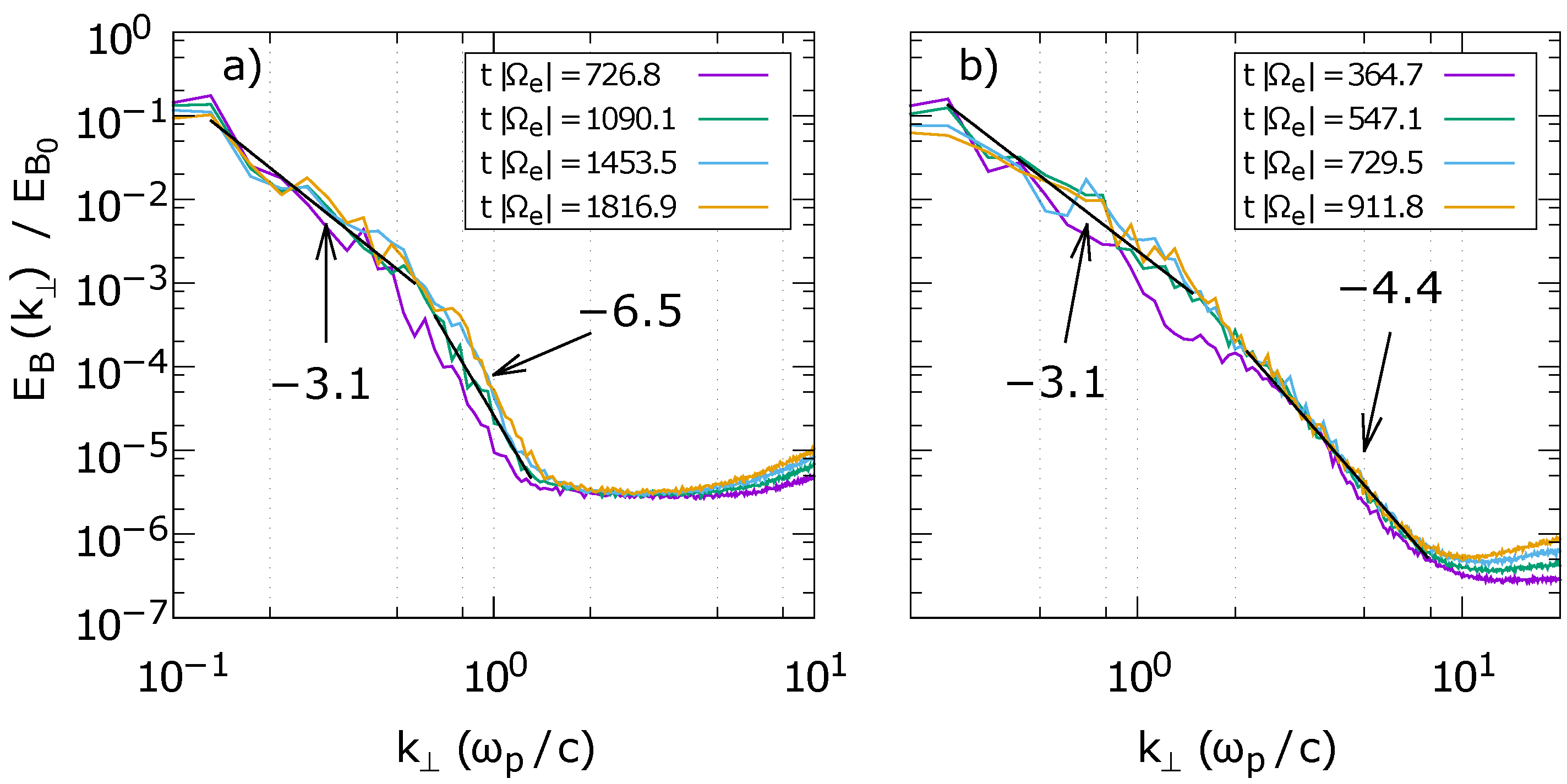
Figure 3 shows the perpendicular spectra of the magnetic field energy from simulations S1 (Figure 3a) and S2 (Figure 3b). At small, perpendicular wave numbers, the magnetic energy distribution follows a power-law with spectral index and for S1 and S2, respectively. After the break, the spectra steepen, and significant differences between both simulations become obvious in the different spectral indices.
The numerical noise level in simulation S2 is about one order of magnitude lower than in S1, which allows an energy cascade to higher wave numbers. This can be explained by the lower plasma temperature in S2, leading to less kinetic energy of the particles and therefore less fluctuations in the electromagnetic fields. The flatter spectrum in S2 (after the break; compared to S1) agrees with results from Chang [30], who reported a more efficient perpendicular energy transport with decreasing plasma beta .
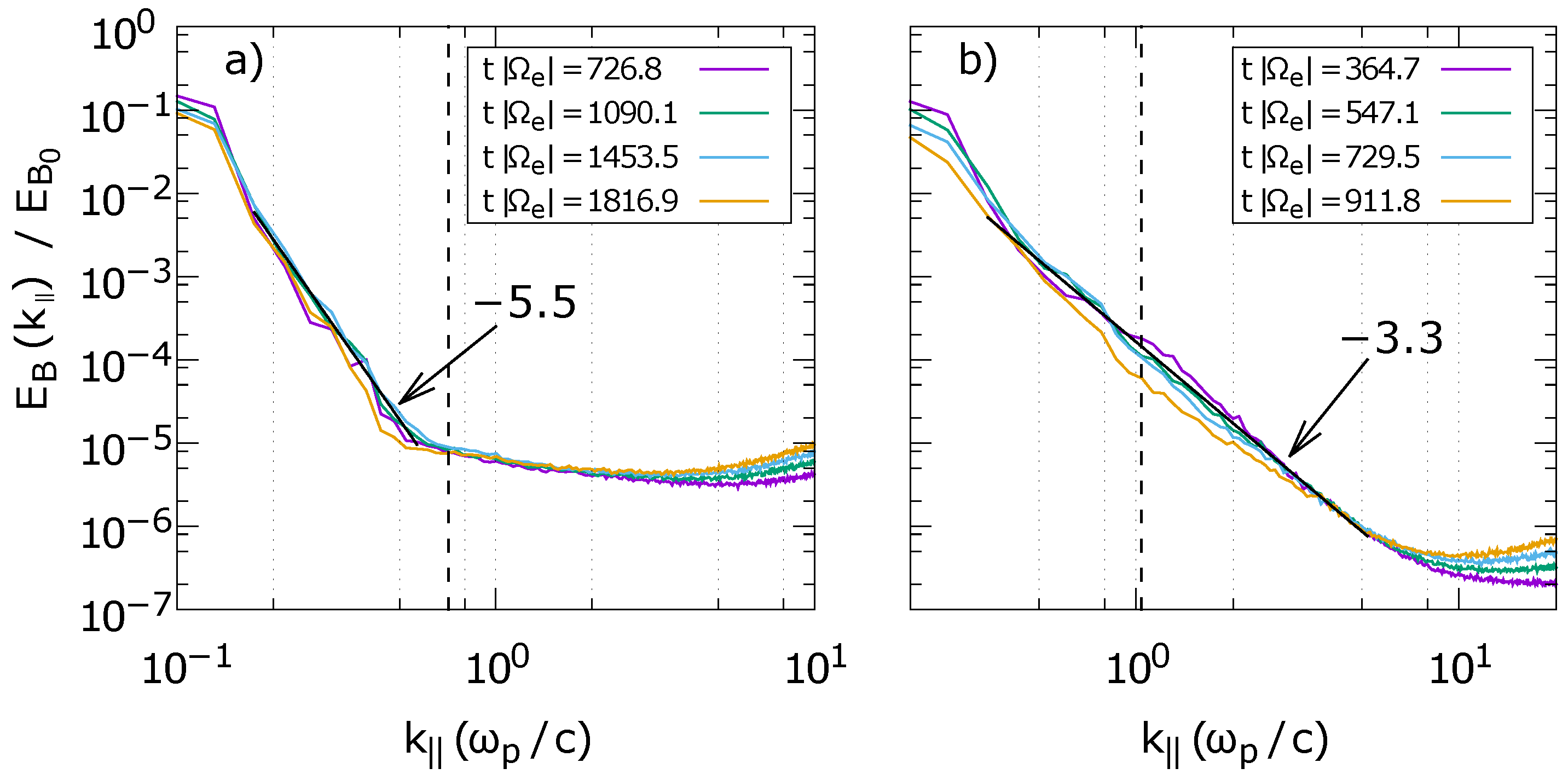
Chang [30] also observed stronger anisotropy in simulations with lower . However, this is not supported by the data from simulations S1 and S2. The parallel spectra are depicted in Figure 4. In both cases, the parallel spectra do not contain a break and are steeper than the perpendicular spectra at small wave numbers. For S1, the parallel spectrum reaches the noise level approximately at the position where cyclotron damping is assumed to set in. Figure 4a,b, however, shows that the parallel spectrum in simulation S2 extends to wave numbers in the damped regime. The slope does not change at the transition into the dissipation range and is flatter than the slope in the perpendicular spectrum at corresponding . Thus, the parallel energy transport is assumed to dominate at large wave numbers. Unfortunately, the turbulent cascade reaches the numerical noise level prior to that.
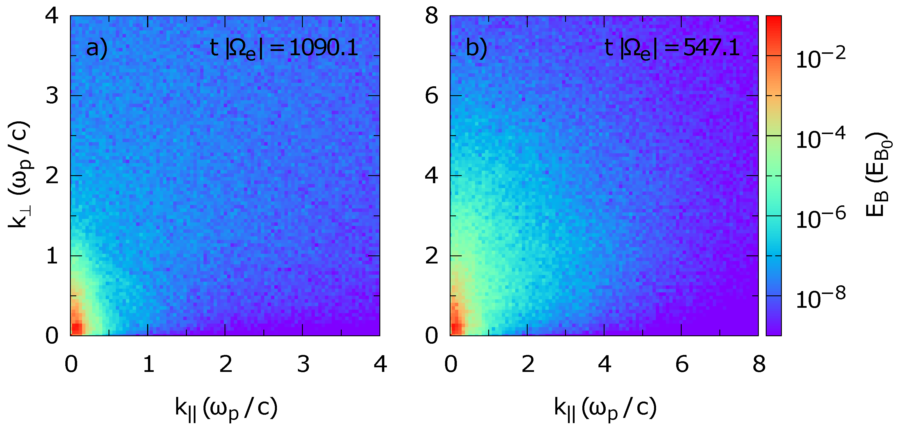
The energy distribution in two-dimensional wave number space supports the claim that parallel energy transport becomes important in simulation S2, as Figure 5 shows. Figure 5b shows the distribution of magnetic field energy in simulation S2. Although hardly any (quasi-)parallel waves are produced above (where cyclotron damping sets in), this critical parallel wave number can be passed at higher . At small wave numbers, however, the perpendicular cascade clearly dominates. In simulation S1, the situation is different, as Figure 5a shows. The perpendicular cascade at small wave numbers is similar to S2, as expected, but at larger , there is hardly any energy transport to higher parallel wave numbers, in agreement with the spectra given in Figure 3 and Figure 4.
3.2. Simulation of Energetic Particles
In order to study wave-particle scattering, a specific initialization of a test particle population is prepared. The ACRONYM code allows for different particle species (typically protons and electrons, but also positrons or heavier ions) and different particle populations (a background plasma and, for example, additional jet populations, non-thermal particles, etc.).
The simulations S1 and S2, discussed here, employ a thermal background plasma (see Table 1) and an additional population of non-thermal test particles to study the transport of energetic electrons. It is found that the test particles have no noticeable influence on the background plasma, even if the ratio of numerical particles in the test to the background particle population is of the order of unity.
3.2.1. Initialization and Analysis
Test particles are initialized as a mono-energetic population; i.e., the particles have the same absolute speed, but their direction of motion is chosen randomly. The speed is calculated from the resonance condition for waves in the plasma. Solving Equation (18) for the speed of a particle of species yields:
where is the desired resonant pitch-angle cosine. The sign in the numerator changes depending on the polarization of the wave, its direction of propagation, and the particle species.
The directions of motion of the bulk of the test particles are chosen at random, using the speed calculated from Equation (47), a random polar angle cosine , and a random azimuth angle . This yields an isotropic distribution of the velocity vectors in - space. It is convenient to choose an isotropic distribution in (instead of ), because the analysis of pitch-angle scattering relies on the pitch-angle cosine and not on the pitch-angle itself.
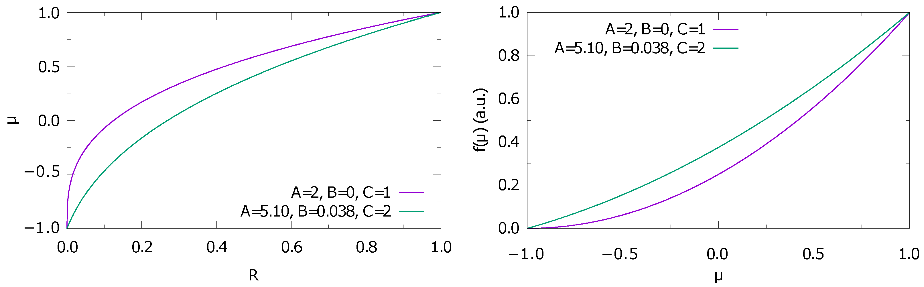
A fraction of the test particle population is not initialized as described above, but instead uses a parabolic distribution of polar angle cosines. This is done by assigning
to the particles, where R is a random number between zero and one, and A, B, and C are parameters describing the shape of the parabola. The parabolic distribution is required for the analysis of pitch-angle scattering using the method of Ivascenko et al. [40]. Ivascenko et al. suggest the use of a half-parabola, i.e., , , , but other distributions are also possible (see Figure 6). The resulting angular distribution of the entire test particle population is, therefore, not entirely isotropic.
The technique described above to create a population of energetic test particles for the study of wave-particle scattering was designed for a single plasma wave in the simulation [41]. However, it can also be applied to simulations with several plasma waves.
The test particle population is not injected at the start of the simulations S1 and S2 but at a later time for the following reason: it is expected that turbulence develops from the initial conditions of the simulation, i.e., from a small set of seed waves that interact and start the turbulent cascade. This process takes time, and it may be desired to wait until a turbulent cascade is established before the transport of energetic test particles can be studied. Therefore, an optional deployment of test particles at later times in the simulation is favored. The particles are created at a a pre-defined time step, and the initialization is carried out as described earlier. Those particles can then be tracked for the rest of the simulation.
To evaluate particle transport in the turbulent plasma, the test particle data can be analyzed after the simulation to obtain the diffusion coefficient . The diffusion coefficient is calculated from a simplified Fokker–Planck equation, Equation (22), where pitch-angle diffusion is assumed to be the only relevant diffusion process:
This equation can be rewritten to yield
The method described by Ivascenko et al. [40] is based on integrating Equation (49) over , which yields the pitch-angle current :
The diffusion coefficient is then obtained by dividing by .
3.2.2. Physical Parameters
Using the setups of simulations S1 and S2, the transport of energetic electrons in kinetic turbulence is studied. In the following, the exact parameters for the test particle energy distribution are presented.
In simulations S1 and S2, decaying whistler turbulence is simulated, as was shown in the Section 3.2. As can be seen in the magnetic energy spectra presented in Figure 3 and Figure 4, a steady state in terms of the power-law slope of the spectral energy distribution is established after a given time in each of the two simulations. As soon as this stage of the simulation is reached, a population of energetic test electrons can be injected as described in Section 3.2.1.
The time step for the checkpoint and subsequent restart is chosen to be for S1 and for S2. For each of these two setups, six test electron configurations are prepared. The simulations are labeled according to the physical setup (S1 or S2) followed by a letter referring to the test particle configuration (“a” through “f”). The parameters of the test particles can be found in Table 3 and describe the test electron speed and kinetic energy .
The test electron energy is increased from simulation S1a (S2a) to S1e (S2e). Simulation S1f (S2f) uses the same particle energy as S1e (S2e), but a different parabolic angular distribution of the particles. Here the particle density increases with increasing , while in the other simulations it decreases with increasing pitch-angle cosine. This change in the pitch-angle distribution allows to check for systematic errors in the particle data.
4. Results
Pitch-Angle Diffusion Coefficients
The test particle simulations are analyzed as described in Section 3.2.1. The energetic electrons are tracked for several electron cyclotron time scales, and the resulting pitch-angle diffusion coefficients are presented in Figure 7 and Figure 8 for data based on the setup of S1 and S2, respectively. Time is measured as the interval from the time of the injection of the particles to the current time step.
The results of both sets of simulations, one based on S1 and the other based on S2, do not differ qualitatively, as would be expected from the two setups. The only difference between the physical parameters for S1 and S2 is the plasma temperature, which has no direct influence on the test electrons. Although the magnetic energy spectrum differs at high wave numbers (see Figure 3), the distribution of magnetic energy at small wave numbers is very similar. As it is explained below, this low-wave-number regime represents the dominant influence on particle transport. Thus, the two sets of simulations are discussed simultaneously in what follows.
Although particle data can be obtained for an arbitrary number of time steps, the interval that can be used for the analysis is still limited. The method of Ivascenko et al. [40] critically depends on the particle distribution in pitch-angle space. In order for the method to work, the initial distribution must be slightly disturbed, but the perturbations must not be too strong. This leaves only a brief period of time for the optimal efficiency of the method.
Figure 7a and Figure 8a show the typical behavior of the derived over time. Shortly after the injection of the test electrons, the perturbations of are small, resulting in a low amplitude of (purple lines). With increasing time, the amplitude grows and reaches a maximum (green and blue lines). At later times, the amplitude decreases again, as the perturbations become too strong and the method becomes unreliable (orange lines). The other panels of the two figures show the time evolution until the maximum amplitude of is reached for other test electron energies.
Although the turbulent cascade is assumed to be symmetric about , the panels of Figure 7 and Figure 8 show an obvious asymmetry in the pitch angle diffusion coefficients derived from the test electron data. The amplitude of is generally larger for . While the energy spectrum itself is isotropic in , one could argue that the polarization of the waves’ magnetic fields relative to the direction of the background magnetic field is different (i.e., the plasma physics definition of the polarization).
The magnetic helicity of the plasma waves is one of the possible causes of this anisotropy. Another reason for the asymmetry found in Figure 7 and Figure 8 is that the parabolic distribution of the test particles implies that there are more test electrons at negative pitch-angle cosines (except for simulations S1f and S2f). Therefore, the particle statistics is more reliable for negative , and the method of Ivascenko et al. [40] produces more accurate diffusion coefficients. While can also be calculated for , it is more prone to errors, and statistical fluctuations play a more important role, as Figure 9 indicates. However, small-scale statistical fluctuations can be suppressed by use of a Savitzky-Golay filter, as suggested by Ivascenko et al. [40].
Especially for early time steps, it can be seen that is found to diverge at . This is, of course, not a physical effect. At , the derivative of the initial parabolic distribution becomes (almost) zero. In this case, the method of Ivascenko et al. [40] becomes numerically unstable.
Another numerical effect causes to become negative. This can be seen in Figure 8d and Figure 8e for early times. Negative solutions are most likely related to statistical fluctuations in the particle distribution, which drown the signal at early times, when the physically motivated perturbations of are still developing.
Besides these flaws, the derived pitch-angle diffusion coefficients appear reasonable. They develop a (more or less) symmetric shape about , indicating that neither direction is preferred. This is expected from the setup of the turbulence simulations S1 and S2, which employ a symmetric layout of initial waves and therefore should produce turbulent cascades that are symmetric in . This, however, cannot be proven by the plots of the energy distribution in wave number space, since the information about the direction of propagation of the waves is lost.
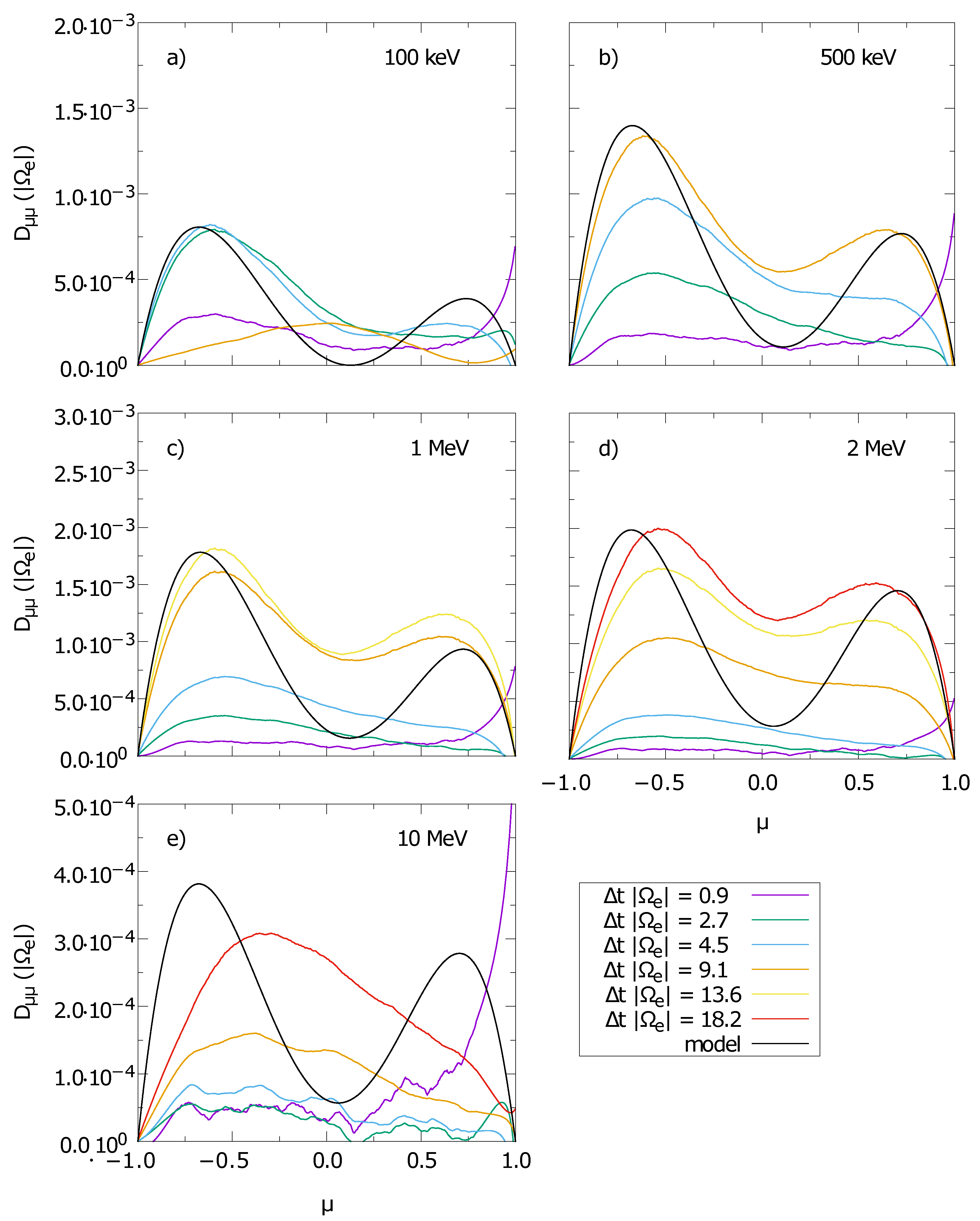
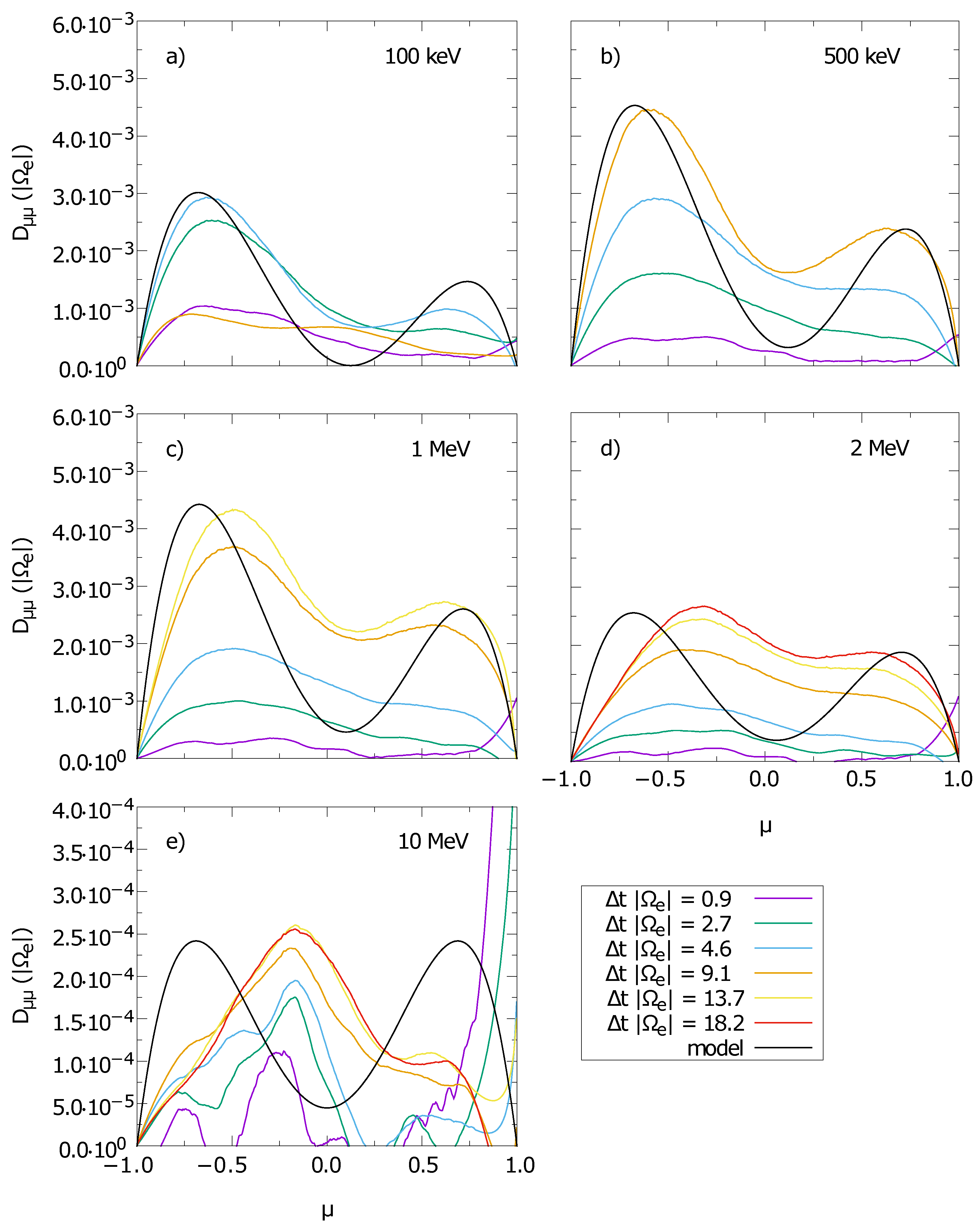
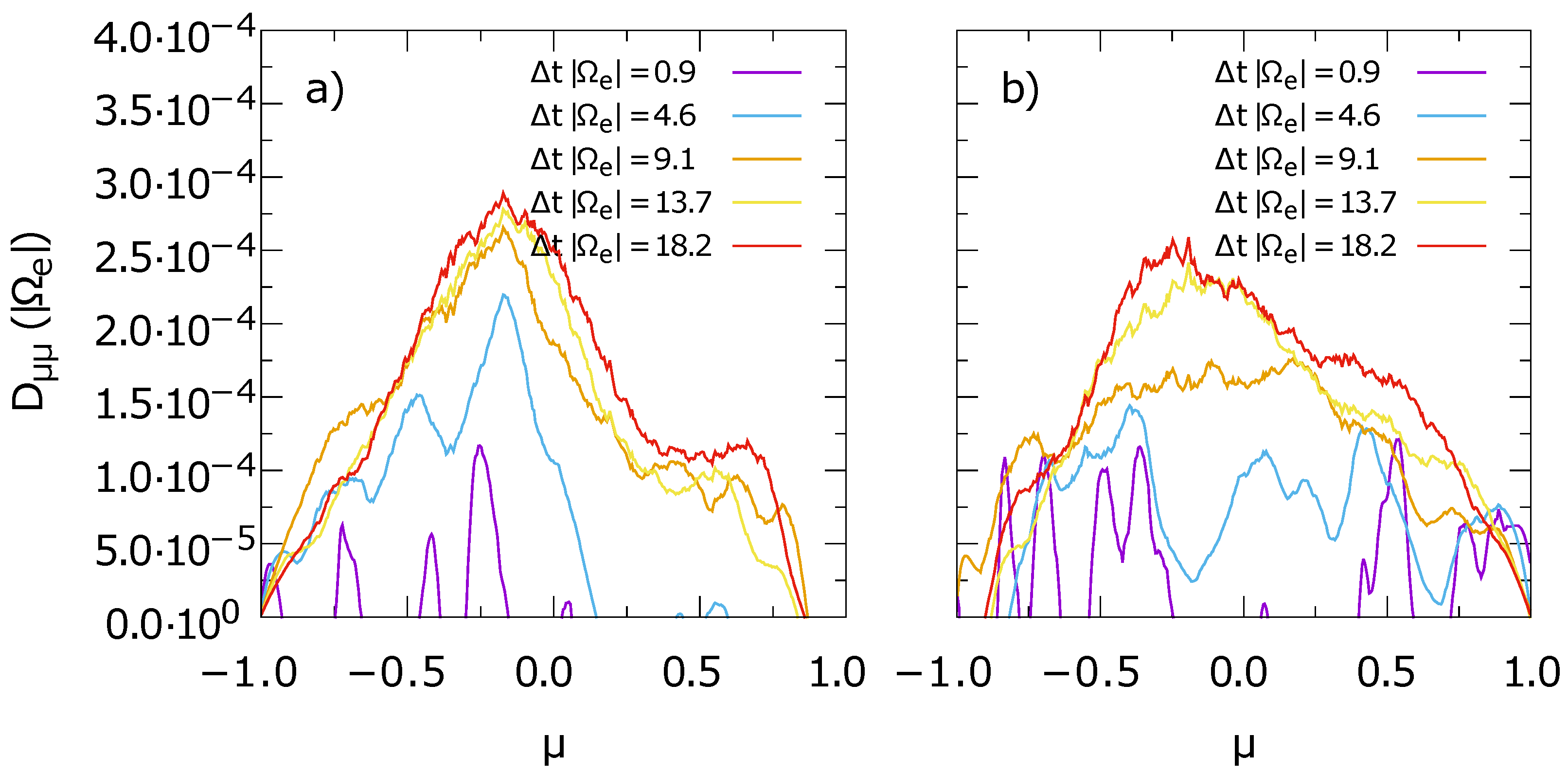
An interesting observation is that the pitch-angle diffusion coefficients grow in amplitude with the particle energy increasing from to . At the highest test electron energy, however, the amplitude of is significantly lower than in all other cases. Both Figure 7e and Figure 8e also show that forms a single peak close to in the case of the highest electron energy, whereas all other simulations produce a double peak structure. The reason for these differences is not clear. However, it is assumed that the different behavior of the electrons is related to their scattering characteristics. These high energy particles resonate with all of the initially excited waves in the simulations (see Figure 2), which is not the case in the simulations of less energetic electrons. Since the initial waves contain the most energy, they are also assumed to significantly influence particle transport, especially if wave–particle resonances may occur.
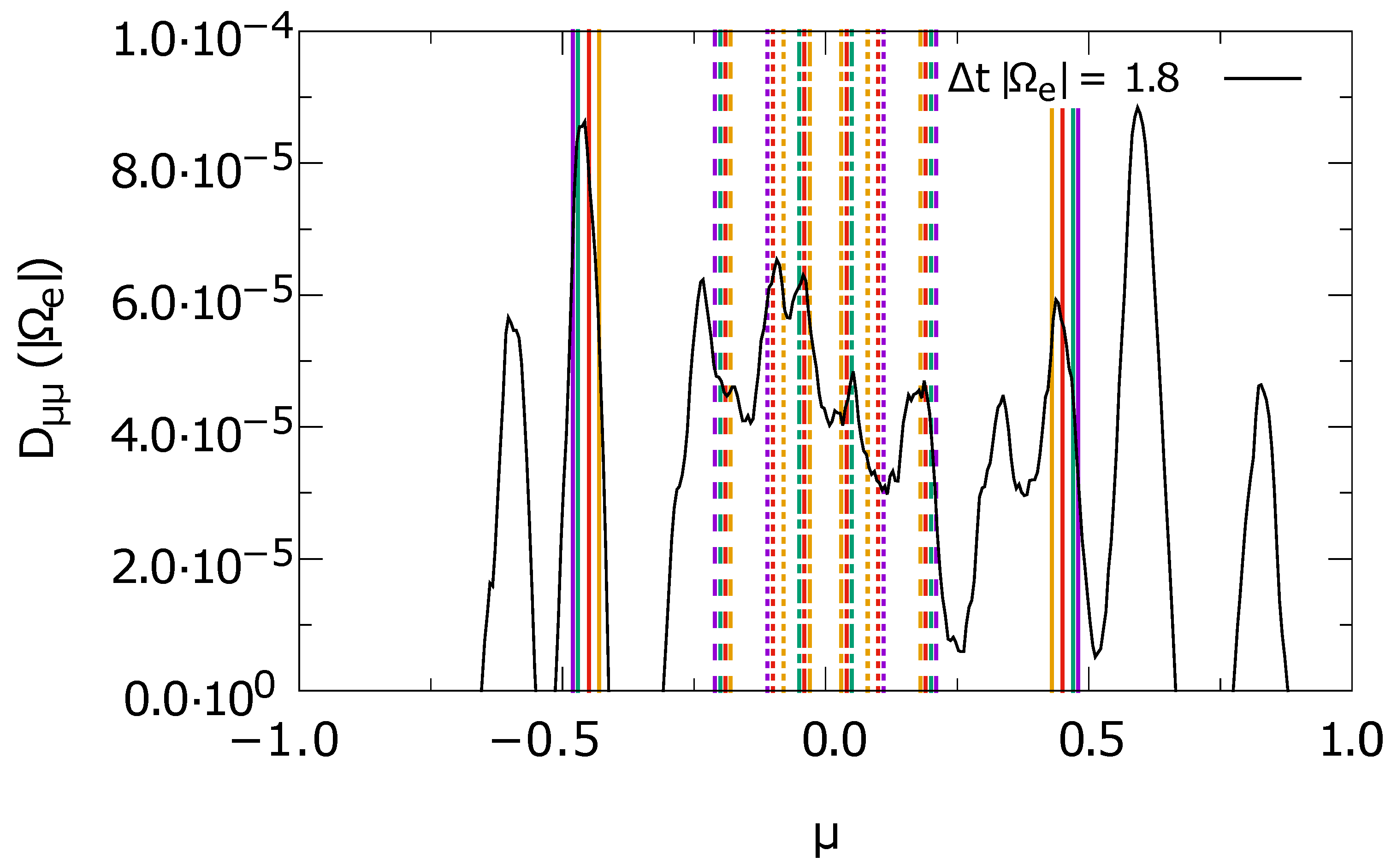
In fact, the in Figure 7e and Figure 8e exhibit distinct peaks at early times (purple and green curves). Similar behavior is also found in simulations S1f and S2f, which are not included in Figure 7 and Figure 8. For the example of one time step in simulation S1f, the peak structures in are related to wave–particle resonances calculated according to Equation (18). The result is shown in Figure 10, where the colored vertical lines mark the expected positions of resonances. It can be seen that the resonances coincide with the positions of the peaks in . The region around is most densely populated by resonances, which might explain the single peak in at later times as seen in Figure 7e and Figure 8e.
Finally, Figure 7 and Figure 8 also include the model predictions from Equations (41) and (42). Some of the parameters required can be directly obtained from the setup of the simulations: the ratio is listed in Table 1, and the test electron speed speed and the electron cyclotron frequency are found in Table 3. However, the minimum wave number , the spectral index s, and the cross helicity and magnetic helicity are not as trivial to find.
For the minimum wave number, the magnetic energy spectra in Figure 3 and Figure 4 have been considered. The second smallest resolved wave number has been chosen, where is the grid spacing in wave number space. In a square simulation box, where the numbers of grid cells and in the parallel and perpendicular directions are equal, the grid spacing is given by . The minimum wave number marks the beginning of the downward slope of the energy spectrum. Waves at small wave numbers are assumed to dominate the interaction with the particles due to their high energy content and the steep spectral slope. Therefore, the spectral index was chosen, in accordance with the index of the perpendicular spectrum in Figure 3a. This spectral index corresponds to simulation S1, but since the index in S2 is similar, was used in both cases.
Finally, the magnetic helicity was chosen to be 0. The effect is in fact rather small since electrons mostly resonate with right-handed polarized modes.
From this starting point, the three parameters , s, and were fitted according to the numerical data from each simulation. The resulting parameters, which are used in the plots in Figure 7 and Figure 8, are listed in Table 4. It can be seen that most simulations can be described with the initial choices for and s explained above.
In general, the model describes the data surprisingly well. Position and amplitude of the maxima and the inclination of the flanks are in good agreement. The contributions at are in disagreement; this is however not unexpected as for quasi-linear theory. Still, a non-zero contribution at medium energies is found, which is different from a non-dispersive quasi-linear approach. The agreement of the model and the simulation results also supports the claim that the waves at small wave numbers dominate the interactions with the particles. Otherwise, the spectral index s would have to be changed according to the particle energy. The low energy particles, e.g., , resonate with plasma waves in the high wave number regime, where the spectrum is steeper. Thus, according to Figure 3 and Figure 4, the effective spectral index s should increase for these particles, if the resonant interactions with high-k waves were important. However, this seems not to be the case. But as the results in Figure 7 and Figure 8 show, a change of the model equations for is not necessary.
The model only fails for the simulations of -electrons (S1e, S1f, S2e, S2f). This might already be expected from the considerations discussed above: the high energy electrons are able to resonate with the initially excited waves. These waves contain the most energy and thus dominate the interaction of the particles with the turbulent spectrum. However, the initial waves cannot be considered to be part of the power-law spectrum itself. As Figure 3 and Figure 4 show, the energy distribution forms a plateau at smallest wave numbers, where the initial waves are located. The initial waves are also only few in number, thus not forming a continuous spectrum but a population of distinct, individual waves. Representing a continuous spectrum on a discretized grid is always doomed to fail, but at larger wave numbers, the higher number of individual waves at least creates a rudimentary approximation of a continuum. Thus, the whole model assumption, i.e., a continuous power-law spectrum, is invalid. As Figure 10 shows, the pitch-angle diffusion coefficient derived from the simulation data can be described reasonably well by individual resonances with a number of waves.
Finally, it is worth taking a look at simulations S1f and S2f, which have not been discussed so far. These simulations, which employ the same test electron energies as S1e and S2e, were carried out to test whether the initial particle distribution has an influence on the resulting . It was already discussed above that the statistical fluctuations tend to become more noticeable at those where fewer particles are located. Thus, reversing the slope of the initial parabola should shift the dominant influence of statistical fluctuations from positive to negative.
Figure 11 depicts the pitch-angle diffusion coefficients derived from simulations S2e and S2f in panels a and b, respectively. This example is chosen because physical results for are only obtained at negative at early times in S2e. Should this also be the case in S2f, this would mean that some physical process prefers the interaction of waves and energetic particles that propagate opposite to the background magnetic field. However, as Figure 11 shows, this is not the case. The pitch-angle diffusion coefficient derived from S2f appears to be more symmetric about at early times.
At late times both simulations produce a single peak in , which is located near . The peak is slightly shifted to negative in both S2e and S2f. This may hint at a physical process leading to the peak not being centered exactly around . Such an asymmetry is sometimes predicted in theoretical models, e.g., Schlickeiser [11]. However, considering the results of simulations of energetic particles and their interaction with individual waves, an asymmetry is not expected here.
Thus, the results of simulations S2e and S2f depicted in Figure 11 do not entirely agree with the expectations. It might be worthwhile to investigate the behavior of the pitch-angle diffusion coefficient in more detail in a future project. Changing the initial particle distribution once more (e.g., by altering the parameters A, B, and C in Equation (48)) or reversing the direction of the integration over in the method of [40] might help to distinguish between a physically motivated asymmetry and numerical artifacts.
5. Conclusions
In this paper, a set of pitch-angle diffusion coefficients for dispersive whistler waves are derived. Using a particle-in-cell code turbulence in the dispersive regime was simulated. Test particle electrons were injected into the simulated turbulence and their transport parameters were derived.
The conducted turbulence simulations yield power-law spectra of the magnetic field energy in wave number space. The measured spectral indices are in agreement with the findings of Refs. [27,29]. Numerical noise limits the energy spectra at high wave numbers, thus hindering the production of an energy cascade in the dissipation range.
While the theory is limited to parallel waves, simulations were performed in two-dimensional wave-number space. The theoretical description of oblique, dispersive waves is not practically doable, while one-dimensional turbulence simulations are not producing an energy cascade. The approximation of a parallel spectrum makes this difference between dimensionalities reasonable.
The simulations of energetic particle transport in kinetic turbulence show that the steep energy spectrum leads to wave–particle interactions primarily in the low wave number regime. While low-energy particles, in principle, resonate with waves in the dispersive or dissipative regime of the turbulent cascade, these interactions are subordinate to interactions with non-resonant waves at lower wave numbers. The reason for this is that the energy content of dispersive waves decreases rapidly with increasing wave number due to the steep power-law spectrum. Thus, the waves at low wave numbers dominate the spectrum as far as particle transport is concerned.
This can be seen when comparing simulation data to the theoretical model. The test electron data from the simulations allows us to derive pitch-angle diffusion coefficients using the method of [40]. The presented model for in plasma turbulence with dispersive waves allows for the prediction of pitch-angle diffusion coefficient for Alfvén and whistler turbulence.
Simulation data and model match rather well for low-energy electrons. Contributions at are not modeled correctly as is expected for a quasi-linear model. The cross-helicity assumed in model parameters may not necessarily represent the cross-helicity of the plasma, but may be to some degree a numerical artifact. At higher electron energies, particles interact with the small number of excited plasma waves, which are used as a seed population for the generation of kinetic turbulence. The resulting does not match the prediction for the interaction with the (continuous) turbulent spectrum but can be explained by resonant scattering with several waves at discrete wave numbers.
In general simulations, dispersive whistler turbulence and the corresponding particle transport are possible but are also still too expensive in terms of computing resources.
Author Contributions
Conceptualization, F.S., C.S. and R.S.; methodology, F.S. and R.S.; software, C.S.; writing—original draft preparation, F.S., C.S. and R.S.; writing—review and editing, F.S., C.S. and R.S.; visualization, F.S. and C.S.; funding acquisition, F.S. All authors have read and agreed to the published version of the manuscript.
Funding
This research was funded by Deutsche Forschungsgemeinschaft (DFG) through Grant No. SP 1124/9.
Institutional Review Board Statement
Not applicable.
Informed Consent Statement
Not applicable.
Data Availability Statement
Not applicable.
Acknowledgments
F.S. would like to thank the Deutsche Forschungsgemeinschaft (DFG) for support through Grant No. SP 1124/9. The authors gratefully acknowledge the data storage service SDS@hd supported by the Ministry of Science, Research and the Arts Baden-Württemberg (MWK) and the German Research Foundation (DFG) through grant INST 35/1314-1 FUGG and INST 35/1503-1 FUGG. The authors gratefully acknowledge the Gauss Centre for Supercomputing e.V. (www.gauss-centre.eu, accessed on 30 November 2021) for funding this project by providing computing time on the GCS Supercomputer SuperMUC at Leibniz Supercomputing Centre (www.lrz.de, accessed on 30 November 2021) through grant pr84ti. We acknowledge the use of the ACRONYM code and would like to thank the developers (Verein zur Förderung kinetischer Plasmasimulationen e.V.) for their support.
Conflicts of Interest
The authors declare no conflict of interest.
References
- Borovsky, J.E.; Funsten, H.O. Role of solar wind turbulence in the coupling of the solar wind to the Earth’s magnetosphere. J. Geophys. Res. Space Phys. 2003, 108, 1246. [Google Scholar] [CrossRef]
- Sridhar, S.; Goldreich, P. Toward a theory of interstellar turbulence. I: Weak Alfvénic turbulence. Astropart. Phys. 1994, 432, 612–621. [Google Scholar] [CrossRef] [Green Version]
- Goldreich, P.; Sridhar, S. Toward a theory of interstellar turbulence. II: Strong Alfvénic turbulence. Astropart. Phys. 1995, 438, 763–775. [Google Scholar] [CrossRef]
- Sahraoui, F.; Goldstein, M.L.; Belmont, G.; Canu, P.; Rezeau, L. Three Dimensional Anisotropic k Spectra of Turbulence at Subproton Scales in the Solar Wind. Phys. Rev. Lett. 2010, 105, 131101. [Google Scholar] [CrossRef] [PubMed]
- Galtier, S.; Nazarenko, S.V.; Newell, A.C.; Pouquet, A. A weak turbulence theory for incompressible magnetohydrodynamics. J. Plasma Phys. 2000, 63, 447–488. [Google Scholar] [CrossRef] [Green Version]
- Galtier, S.; Nazarenko, S.V.; Newell, A.C.; Pouquet, A. Anisotropic Turbulence of Shear-Alfvén Waves. Astrophys. J. 2002, 564, L49–L52. [Google Scholar] [CrossRef]
- Howes, G.G. Kinetic turbulence. In Magnetic Fields in Diffuse Media; Lazarian, A., de Gouveia Dal Pino, E., Melioli, C., Eds.; Springer: Berlin/Hedelberg, Germany, 2015; pp. 123–152. [Google Scholar] [CrossRef]
- Gary, S.P.; Smith, C. Short-wavelength turbulence in the solar wind: Linear theory of whistler and kinetic Alfvén fluctuations. J. Geophys. Res. 2009, 114, A12105. [Google Scholar] [CrossRef]
- Jokipii, J.R. Cosmic-Ray Propagation. I. Charged Particles in a Random Magnetic Field. Astrophys. J. 1966, 146, 480–487. [Google Scholar] [CrossRef]
- Lee, M.A.; Lerche, I. Waves and Irregularities in the Solar Wind. Rev. Geophys. Space Phys. 1974, 12, 671–687. [Google Scholar] [CrossRef]
- Schlickeiser, R. Cosmic-ray transport and acceleration. I-Derivation of the kinetic equation and application to cosmic rays in static cold media. II-Cosmic rays in moving cold media with application to diffusive shock wave acceleration. Astrophys. J. 1989, 336, 243–293. [Google Scholar] [CrossRef]
- Steinacker, J.; Miller, J.A. Stochastic gyroresonant electron acceleration in a low-beta plasma. I—Interaction with parallel transverse cold plasma waves. Astrophys. J. 1992, 393, 764–781. [Google Scholar] [CrossRef]
- Vainio, R. Charged-Particle Resonance Conditions and Transport Coefficients in Slab-Mode Waves. Astrophys. J. Suppl. Ser. 2000, 131, 519. [Google Scholar] [CrossRef] [Green Version]
- Achatz, U.; Dröge, W.; Schlickeiser, R.; Wibberenz, G. Interplanetary transport of solar electrons and protons: Effect of dissipative processes in the magnetic field power spectrum. J. Geophys. Res. 1993, 98, 13261–13280. [Google Scholar] [CrossRef]
- Ng, C.K.; Reames, D.V. Focused interplanetary transport of approximately 1 MeV solar energetic protons through self-generated Alfvén waves. Astrophys. J. 1994, 424, 1032–1048. [Google Scholar] [CrossRef]
- Vainio, R.; Kocharov, L. Proton transport through self-generated waves in impulsive flares. Astron. Astrophys. 2001, 375, 251–259. [Google Scholar] [CrossRef] [Green Version]
- Lange, S.; Spanier, F.; Battarbee, M.; Vainio, R.; Laitinen, T. Particle scattering in turbulent plasmas with amplified wave modes. Astron. Astrophys. 2013, 553, A129. [Google Scholar] [CrossRef] [Green Version]
- Gary, S.P.; Saito, S. Particle-in-cell simulations of Alfvén-cyclotron wave scattering: Proton velocity distributions. J. Geophys. Res. 2003, 108, 1194. [Google Scholar] [CrossRef]
- Camporeale, E. Resonant and nonresonant whistlers-particle interaction in the radiation belts. Geophys. Res. Lett. 2015, 42, 3114–3121. [Google Scholar] [CrossRef] [Green Version]
- Ma, C.Y.; Summers, D. Formation of power-law energy spectra in space plasmas by stochastic acceleration due to whistler-mode waves. Geophys. Res. Lett. 1998, 25, 4099–4102. [Google Scholar] [CrossRef] [Green Version]
- Dröge, W. Particle Scattering by Magnetic Fields. In Cosmic Rays and Earth: Proceedings of the an ISSI Workshop, Bern, Switzerland, 21–26 March 1999; Bieber, J.W., Eroshenko, E., Evenson, P., Flückiger, E.O., Kallenbach, R., Eds.; Springer: Dordrecht, The Netherlands, 2000; pp. 121–151. [Google Scholar] [CrossRef]
- Coroniti, F.V.; Kennel, C.F.; Scarf, F.L. Whistler mode turbulence in the disturbed solar wind. J. Geophys. Res. 1982, 87, 6029–6044. [Google Scholar] [CrossRef]
- Aguilar-Rodriguez, E.; Blanco-Cano, X.; Russel, C.T.; Luhmann, J.G.; Jian, L.K.; Ramírez Vélez, J.C. Dual observations of the interplanetary shocks associated with stream interaction regions. J. Geophys. Res. 2011, 116, A12109. [Google Scholar] [CrossRef] [Green Version]
- Fairfield, D.H. Whistler waves observed upstream from collisionless shocks. J. Geophys. Res. 1974, 79, 1368–1378. [Google Scholar] [CrossRef]
- Kennel, C.; Petschek, H. Limit on stably trapped particle fluxes. J. Geophys. Res. 1966, 71, 1–28. [Google Scholar] [CrossRef] [Green Version]
- Palmroth, M.; Archer, M.; Vainio, R.; Hietala, H.; Pfau-Kempf, Y.; Hoilijoki, S.; Hannuksela, O.; Ganse, U.; Sandroos, A.; von Alfthan, S.; et al. ULF foreshock under radial IMF: THEMIS observations and global kinetic simulation Vlasiator results compared. J. Geophys. Res. Space Phys. 2015, 120, 8782–8798. [Google Scholar] [CrossRef]
- Gary, S.P.; Saito, S.; Li, H. Cascade of whistler turbulence: Particle-in-cell simulations. Geophys. Res. Lett. 2008, 35. [Google Scholar] [CrossRef]
- Che, H.; Goldstein, M.L.; Viñas, A.F. Bidirectional energy cascades and the origin of kinetic Alfvénic and whistler turbulence in the solar wind. Phys. Rev. Lett. 2014, 112, 061101. [Google Scholar] [CrossRef] [PubMed] [Green Version]
- Gary, S.P.; Chang, O.; Wang, J. Forward cascade of whistler turbulence: Three-dimensional particle-in-cell simulations. Astrophys. J. 2012, 755, 142. [Google Scholar] [CrossRef] [Green Version]
- Chang, O.; Gary, S.P.; Wang, J. Whistler turbulence at variable electron beta: Three-dimensional particle-in-cell simulations. J. Geophys. Res. Space Phys. 2013, 118, 2824–2833. [Google Scholar] [CrossRef]
- Gary, S.P.; Hughes, R.S.; Wang, J.; Chang, O. Whistler anisotropy instability: Spectral transfer in a three-dimensional particle-in-cell simulation. J. Geophys. Res. Space Phys. 2014, 119, 1429–1434. [Google Scholar] [CrossRef]
- Chang, O.; Gary, S.P.; Wang, J. Whistler Turbulence Forward Cascade versus Inverse Cascade: Three-dimensional Particle-in-cell Simulations. Astrophys. J. 2015, 800, 87. [Google Scholar] [CrossRef] [Green Version]
- Schlickeiser, R.; Achatz, U. Cosmic-ray particle transport in weakly turbulent plasmas. Part 1. Theory. J. Plasma Phys. 1993, 49, 63–77. [Google Scholar] [CrossRef]
- Swanson, D.G. Plasma Waves; Academic Press: San Diego, CA, USA, 1989. [Google Scholar] [CrossRef]
- Schlickeiser, R. Cosmic Ray Astrophysics; Springer: Berlin/Heidelberg, Germany, 2002. [Google Scholar] [CrossRef]
- Terry, P.W.; Almagri, A.F.; Fiksel, G.; Forest, C.B.; Hatch, D.R.; Jenko, F.; Nornberg, M.D.; Prager, S.C.; Rahbarnia, K.; Ren, Y.; et al. Dissipation range turbulent cascades in plasmasa. Phys. Plasmas 2012, 19, 055906. [Google Scholar] [CrossRef]
- Hockney, R.W.; Eastwood, J.W. Computer Simulation Using Particles; CRC Press/Taylor & Francis Group: Boca Raton, FL, USA, 1988. [Google Scholar] [CrossRef]
- Kilian, P.; Burkart, T.; Spanier, F. The influence of the mass ratio on particle acceleration by the filamentation instability. In High Performance Computing in Science and Engineering’11; Nagel, W.E., Kröner, D.B., Resch, M., Eds.; Springer: Berlin/Heidelberg, Germany, 2012; pp. 5–13. [Google Scholar] [CrossRef]
- Schreiner, C.; Spanier, F. Wave-particle-interaction in kinetic plasmas. Comput. Phys. Commun. 2014, 185, 1981–1986. [Google Scholar] [CrossRef] [Green Version]
- Ivascenko, A.; Lange, S.; Spanier, F.; Vainio, R. Determining pitch-angle diffusion coefficients from test particle simulation. Astrophys. J. 2016, 833, 223–231. [Google Scholar] [CrossRef] [Green Version]
- Schreiner, C.; Kilian, P.; Spanier, F. Particle scattering off of right-handed dispersive waves. Astrophys. J. 2017, 834, 161–179. [Google Scholar] [CrossRef] [Green Version]
Figure 1.
The pitch-angle dependence of the Fokker–Planck scattering coefficient model calculation for electrons at extreme ends. A power-law spectrum with with spectral index in the wave number range , where M is the proton-to-electron mass ratio, is assumed. Electrons at and are considered. The proton gyrofrequency Hz, and the Alfvén speed in fractions of the speed of light c.

Figure 2.
Schematic representation of two-dimensional wave number space. The discretized wave vectors are represented by the gray boxes, and the axes mark the directions parallel () and perpendicular () to the background magnetic field in the case of a two-dimensional simulation. For the simulation of decaying turbulence in two dimensions, a set of 42 initial waves is excited, where each wave occupies one position on the grid. These positions are indicated by the blue boxes in accordance with the setup specified by Gary [27].

Figure 3.
Normalized magnetic field energy distribution over the perpendicular wave number, normalized to , for simulations S1 (a) and S2 (b). Here, is the magnetic field energy of the background, is the plasma frequency, and c is the speed of light. The data are obtained at four times as indicated, where is the electron gyrofrquency. At the earliest time steps, the spectra reach their steady states. Later in the simulations, the shapes of the spectra do not change significantly. Power-law fits to the data are indicated by the black lines at times (a) and 547.1 (b). The corresponding spectral indices are highlighted by the arrows.

Figure 4.
Normalized magnetic field energy distribution over the parallel wave number, normalized to , for simulations S1 (a) and S2 (b). The data are obtained at four times as indicated. The spectra reach their steady state at the earliest time steps. Power-law fits to the data are indicated by the black lines at times (a) and 547.1 (b). The spectral indices are highlighted by the arrows. The dashed vertical lines indicatethe expected onset of cyclotron damping for purely parallel propagating waves.

Figure 5.
Two-dimensional magnetic field energy distribution in wave number space for simulations S1 (a) and S2 (b). Note different scales on the axes of (a) vs. (b).
Figure 5.
Two-dimensional magnetic field energy distribution in wave number space for simulations S1 (a) and S2 (b). Note different scales on the axes of (a) vs. (b).

Figure 6.
A fraction of the test particle population has pitch-angle cosines assigned according to a parabolic distribution. Left panel: the assigned pitch-angle cosine as a function of the random number , which is used to generate the distribution. The curves follow Equation (48) and employ two sets of parameters A, B, and C, as indicated. Right panel: the resulting particle distribution as a function of . The purple lines employ the parameters suggested by Ivascenko et al. [40], whereas the green curves show an improved implementation that is used in the ACRONYM code. Note that the derivative over the whole range of pitch-angle cosines in the latter case, whereas it becomes zero at when the parameters of Ivascenko et al. [40] are used.

Figure 7.
Pitch-angle diffusion coefficients for test electrons with different energies for simulations S1a to S1e (a–e). The colored lines denote the diffusion coefficients derived from the simulation data at various times. The black lines represent the model predictions derived in Section 2.3.3.
Figure 7.
Pitch-angle diffusion coefficients for test electrons with different energies for simulations S1a to S1e (a–e). The colored lines denote the diffusion coefficients derived from the simulation data at various times. The black lines represent the model predictions derived in Section 2.3.3.

Figure 8.
Pitch-angle diffusion coefficients for test electrons with different energies for simulations S2a to S2e (a–e). The colored lines denote the diffusion coefficients derived from the simulation data at various times. The black lines follow the model predictions derived in Section 2.3.3.
Figure 8.
Pitch-angle diffusion coefficients for test electrons with different energies for simulations S2a to S2e (a–e). The colored lines denote the diffusion coefficients derived from the simulation data at various times. The black lines follow the model predictions derived in Section 2.3.3.

Figure 9.
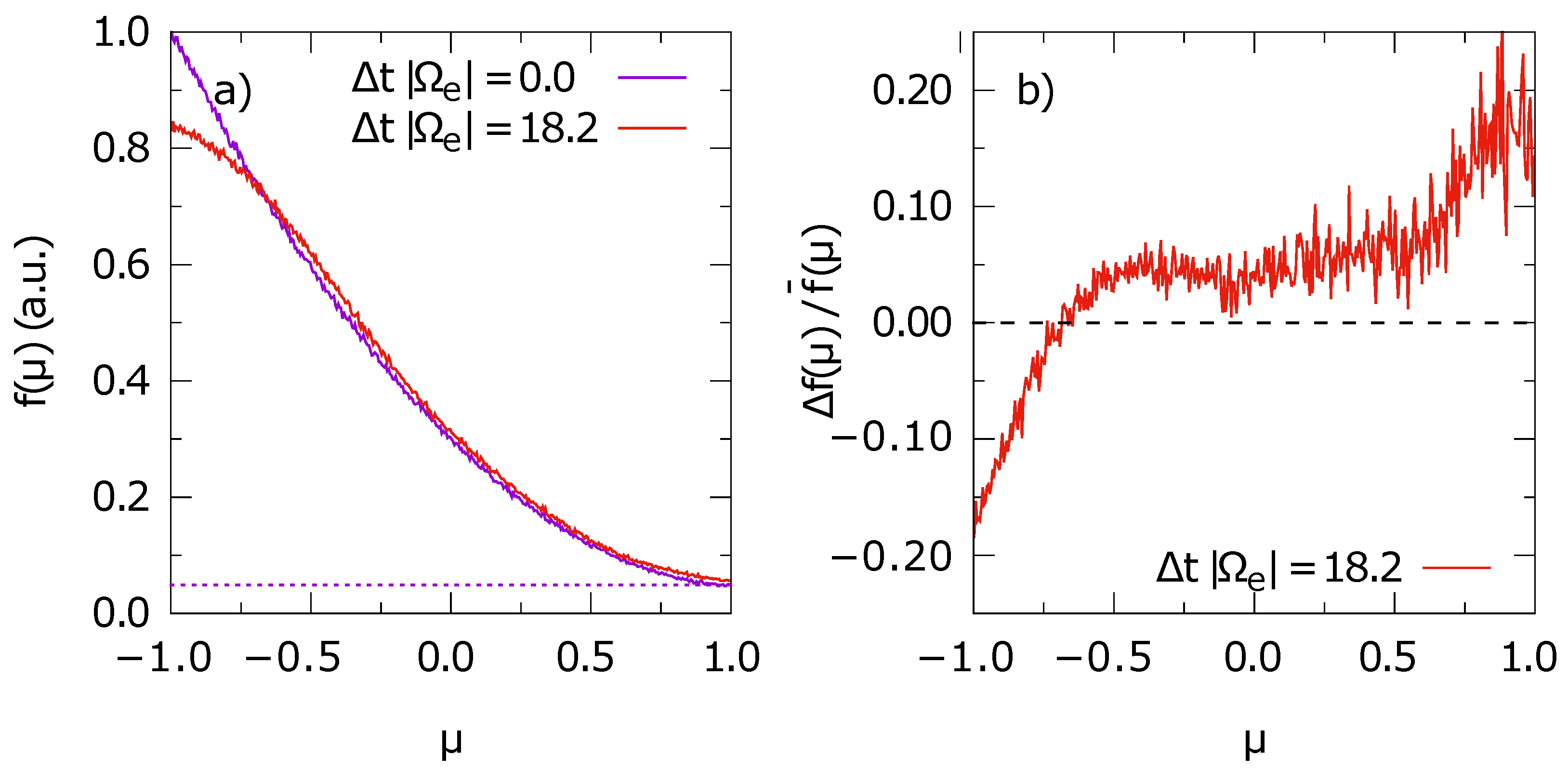
Test electron distribution in pitch-angle space: (a) the initial distribution at the time of the injection of the test electrons () and at a later time in simulation S1c; (b) the relative deviation of the distributions at these two time steps. The deviation is defined as the difference of the two distributions over their mean value. Statistical fluctuations are visible to become more significant for larger values.
Figure 9.
Test electron distribution in pitch-angle space: (a) the initial distribution at the time of the injection of the test electrons () and at a later time in simulation S1c; (b) the relative deviation of the distributions at these two time steps. The deviation is defined as the difference of the two distributions over their mean value. Statistical fluctuations are visible to become more significant for larger values.

Figure 10.
Pitch-angle diffusion coefficient at one point in time as derived from the data of simulation S1f (black line). A noticeable number of peaks in coincide with the positions of wave–particle resonances predicted by the resonance condition (18), which are marked by the colored, vertical lines. The colors denote the parallel wave numbers (in numerical units) from one to four: purple, green, red, and orange. The line style refers to perpendicular wave numbers (also in numerical units) from zero to three: solid, dashed, dotted, dot-dashed. For example, the red dashed lines represent the resonance with a wave at . Only resonances of the first order, i.e., in Equation (18), are shown. Note that does not enter the resonance condition explicitly but is required to calculate the frequency according to the cold plasma dispersion relation.

Figure 11.
Comparison of the pitch-angle diffusion coefficients derived from the test electron data of simulations S2e (a) and S2f (b). The two simulations differ by the slope of the parabolic particle distribution used to initialize the test electrons. The asymmetry of in S2e at early times is not reproduced by S2f, which suggests a numerical or statistical reason for the asymmetry. At late times, the become similar, with a single peak near in both simulations.


Table 1.
Physical parameters for simulations S1 and S2: electron plasma frequency, electron cyclotron frequency, , and thermal speed, of electrons, sum of the squares of the magnetic field amplitudes of the individual waves, and plasma beta .
Table 1.
Physical parameters for simulations S1 and S2: electron plasma frequency, electron cyclotron frequency, , and thermal speed, of electrons, sum of the squares of the magnetic field amplitudes of the individual waves, and plasma beta .
| Simulation | |||||
|---|---|---|---|---|---|
| S1 | 1.966 × 10 | ||||
| S2 |
Table 2.
Numerical parameters for the two-dimensional simulations S1 and S2: number of cells, and , in the directions parallel and perpendicular to the background magnetic field, respectively; number of time steps, , grid spacing, , time step length , and the number of particles (electrons and protons combined) per cell (ppc).
| Simulation | ppc | |||||
|---|---|---|---|---|---|---|
| S1 | 2048 | 2048 | 256 | |||
| S2 | 2048 | 2048 | 256 |
Table 3.
Test electron characteristics for the simulations of particle transport: test electron speed and corresponding kinetic energy . The individual simulations (letters “a” through “f”) are based on the simulations of kinetic turbulence Sj with and 2, which are described in Section 3.1.2 (Table 1 and Table 2). Note that simulations Sje and Sjf employ the same test electron energies. However, they differ in the way the test electron distribution is initialized (see text).
| Simulation | Sja | Sjb | Sjc | Sjd | Sje | Sjf |
|---|---|---|---|---|---|---|
Table 4.
Parameters assumed for the model: spectral index s, cross-helicity , and minimum wave number . The latter is given in units of the grid spacing in wave number space in simulations S1 and S2, respectively.
Table 4.
Parameters assumed for the model: spectral index s, cross-helicity , and minimum wave number . The latter is given in units of the grid spacing in wave number space in simulations S1 and S2, respectively.
| Simulation | S1a | S1b | S1c | S1d | S1e | S1f | S2a | S2b | S2c | S2d | S2e | S2f |
|---|---|---|---|---|---|---|---|---|---|---|---|---|
| s | ||||||||||||
| 0 | 0 | |||||||||||
| 2 | 2 | 2 | 2 | 1 | 1 | 2 | 2 | 2 | 2 | 1 | 1 |
Publisher’s Note: MDPI stays neutral with regard to jurisdictional claims in published maps and institutional affiliations. |
© 2022 by the authors. Licensee MDPI, Basel, Switzerland. This article is an open access article distributed under the terms and conditions of the Creative Commons Attribution (CC BY) license (https://creativecommons.org/licenses/by/4.0/).
Share and Cite
MDPI and ACS Style
Spanier, F.; Schreiner, C.; Schlickeiser, R. Determining Pitch-Angle Diffusion Coefficients for Electrons in Whistler Turbulence. Physics 2022, 4, 80-103. https://0-doi-org.brum.beds.ac.uk/10.3390/physics4010008
AMA Style
Spanier F, Schreiner C, Schlickeiser R. Determining Pitch-Angle Diffusion Coefficients for Electrons in Whistler Turbulence. Physics. 2022; 4(1):80-103. https://0-doi-org.brum.beds.ac.uk/10.3390/physics4010008
Chicago/Turabian StyleSpanier, Felix, Cedric Schreiner, and Reinhard Schlickeiser. 2022. "Determining Pitch-Angle Diffusion Coefficients for Electrons in Whistler Turbulence" Physics 4, no. 1: 80-103. https://0-doi-org.brum.beds.ac.uk/10.3390/physics4010008