A Review on Scene Prediction for Automated Driving


1
Institute of Computer Science, Hochschule Ruhr West, 45479 Mülheim an der Ruhr, Germany
2
Division Electronics and ADAS, ZF Automotive Germany GmbH, 45881 Gelsenkirchen, Germany
3
Institute of Control Theory and Systems Engineering, TU Dortmund University, 44227 Dortmund, Germany
4
Automated Driving & Integral Cognitive Safety, ZF Automotive GmbH, 40547 Düsseldorf, Germany
*
Author to whom correspondence should be addressed.
Physics 2022, 4(1), 132-159; https://0-doi-org.brum.beds.ac.uk/10.3390/physics4010011
Submission received: 1 November 2021
/
Revised: 4 January 2022
/
Accepted: 7 January 2022
/
Published: 1 February 2022
(This article belongs to the Special Issue A Themed Issue in Honor of Professor Reinhard Schlickeiser on the Occasion of His 70th Birthday)
Abstract
:Towards the aim of mastering level 5, a fully automated vehicle needs to be equipped with sensors for a 360 surround perception of the environment. In addition to this, it is required to anticipate plausible evolutions of the traffic scene such that it is possible to act in time, not just to react in case of emergencies. This way, a safe and smooth driving experience can be guaranteed. The complex spatio-temporal dependencies and high dynamics are some of the biggest challenges for scene prediction. The subtile indications of other drivers’ intentions, which are often intuitively clear to the human driver, require data-driven models such as deep learning techniques. When dealing with uncertainties and making decisions based on noisy or sparse data, deep learning models also show a very robust performance. In this survey, a detailed overview of scene prediction models is presented with a historical approach. A quantitative comparison of the model results reveals the dominance of deep learning methods in current state-of-the-art research in this area, leading to a competition on the cm scale. Moreover, it also shows the problem of inter-model comparison, as many publications do not use standardized test sets. However, it is questionable if such improvements on the cm scale are actually necessary. More effort should be spent in trying to understand varying model performances, identifying if the difference is in the datasets (many simple situations versus many corner cases) or actually an issue of the model itself.
1. Introduction
In the last five years, huge progress has been made in the technology of self-driving cars. Advanced Driver Assistance Systems (ADAS) have become very mature and are part of any new vehicle nowadays. First, functions beyond the ADAS level, e.g., lane keeping or lane change assistance, were introduced into the series market of conventional Original Equipment Manufactures (OEMs). Even more compelling were the advances in higher automated driving levels made by Tesla with the autopilot and full self-driving capability functions [1], even though, other than the feature’s names would suggest, the driver is still responsible and needs to monitor the driving process at all times.
The Society of Automotive Engineers (SAE) defines [2] six levels of Automated Driving (AD) (see Figure 1). ADAS systems are limited to levels 1 and 2, where the human driver is still the one operating the vehicle. Although the system can take full control already for specific use cases at level 2, the human driver needs to be attentive all the time, meaning eyes on the traffic at any time. It allows for temporary hands-off but the system reminds the driver to take back control after a short time period.
The actual AD use case starts from level 3. The challenging task in designing a level 3 system is that a human driver who can go hands- and eyes-off must be notified on time to take back control in a period of around 10 s. Bridging the time span of 10 s in case of a complex situation is a great challenge such that some OEMs are discussing the strategy of skipping this level, going straight to high automation level 4. Here, in contrast to the reaction times of human drivers, the vehicle can handle problems on its own within just fractions of a second, or go to a fail-safe condition if no other solutions can be found. The final level 5 can handle all kinds of situations and use cases. A steering wheel might not be present anymore.
In 2019, the first autonomous taxi fleets were announced for the year 2020 [3]. However, this was delayed partially due to legislation and partially due to technical issues. Only slowly, the first test cases have been introduced. While the use case automated highway driving or level 4 driving on well-defined urban test fields can be handled quite well already, the big challenge is handling fully AD level 5 for all possible scenarios and corner cases. This includes strongly populated cities where it is not possible to anticipate the traffic scene for more than 1–2 s reliably or situations that occur very seldom.
The advantages of AD are numerous and quite obvious: an increase in comfort for the passengers, along with more flexibility for young, old or disabled persons. Furthermore, AD will reduce the number of accidents. A simulation study of fatal crashes predicted a reduction of collisions by 82% [4]. Naturally, also machines will fail but the amount and severeness of accidents is expected to be less compared to human drivers. This aspect is followed by a number of ethical questions, e.g., how to decide which action to take in case of an unavoidable crash? This is still a question under discussion. Moreover, human failures are better accepted than accidents caused by a machine. A further advantage to mention is that driverless systems can be optimized in economic aspects. Car sharing concepts are being designed which will reduce the number of required vehicles by efficient usage and fewer parking spaces will be needed. Traffic jams often occur due to inattentive drivers and unnecessary braking maneuvers [5]. This can easily be avoided in driverless traffic with the help of car-to-car communication [6].
While trying to reach the goal of fully automated vehicles, it is important having in mind the demands of the industry. First, AD vehicles need to be equipped with multiple sensors. However, the costs need to be low enough that either individual rides with a robotaxi service or the purchase of an actual automated vehicle is affordable, which obviously addresses people of different income classes. Second, current systems are often requiring high-performing computer hardware. The aim is to go towards embedded systems which are drastically limited in run-time and memory. Last but not least, an AD system has to be robust and secure, meaning that faulty sensors or adversarial attacks [7,8] need to be handled reliably. In order to get permission to drive on public roads, a company needs to undergo a formal procedure that guarantees the functional safety of the system. This latter topic is not trivial and is still a road blocker for bringing some technical applications to the market.
Despite the recent advances in AD, there still exist challenges which are some of the main reasons why fully AD cars cannot be brought onto the streets yet. One of the most challenging problems focused on in this review and being a field of increasingly active research is the prediction of future traffic participants’ behavior. The intentions that lead to certain maneuvers or actions are not always obvious but rather hidden as latent factors. Being able to identify such intentions several seconds before the event, makes it possible to comfortably adjust the own driving trajectory.
A second major challenge is the handling of uncertainties. The perception of the environment is associated with uncertainties, especially when fusing information from different sources. On the one hand, multiple signals provide redundancy and thus more reliability, on the other hand, creating higher uncertainties if the individual signals do not match. Based on these signals, robust environment models need to be developed for a planning of the ego vehicle trajectory. The problem is highly complex and dynamic due to unpredictable external factors, e.g., changing weather conditions, varying environments possibly without road marking or sudden movements of humans and cyclists. Deep learning techniques are quite robust against these uncertainties.
Scene prediction is a field of active research with increasing interest as can be seen from Figure 2. In the following, this review is delimited from previous surveys. Surveys on AD often focus on perception issues and challenges related to fusion of different sources [9,10,11] or psychological aspects related to the interaction between the human driver and the machine [12,13,14]. Some earlier surveys of scene prediction give a good overview of the different approaches but do not consider yet advanced deep learning techniques [15,16]. The review by Xue et al. [17]. focuses on scene understanding, event reasoning and intention prediction, distinguishing between short-term predictions (time horizon of a few seconds) and long-term predictions (time horizon of several minutes) but is kept on a rather high level in terms of methodology.
Scene prediction often takes over new deep learning techniques from the field of natural language processing, a fast moving research area where huge progress has been made in the last three years. Naturally, those latest techniques are contained only in the most recent reviews. Refs. [19,20] highlight the importance of deep learning models but put emphasis on the visual information as input source, such as feature extraction from 3-dimensional (3D) images and videos. In the study by Yin et al. [21] and Tedjopurnomo et al. [22], deep learning techniques are presented in detail but the evaluation is done for traffic flow models. Such models have a time horizon of several minutes in contrast to the models in the paper at hand which are on the horizon of up to 10 s.
In contrast to the paper by Rasouli [23], where a detailed overview of state-of-the-art deep learning techniques is also presented, here, the approach of a historical review is chosen by analyzing the development of the methodology in this field of research. A comparison of the model results reveals the dominance of neural networks in current state-of-the-art methods. We experience the difficulty of quantitative inter-model comparison from [23] since many models are not evaluated on standardized test datasets. However, the value of a competition of performance improvements on the cm scale is questioned here. The focus should be rather on understanding the reasons for significantly varying performances on different datasets which has not been addressed in detail yet.
The review starts with a concise introduction to AD in Section 2 with the aim of placing scene prediction in the context of AD and describing the challenges. In Section 3, the standard models for scene prediction are presented. The historical context and major achievements in scene prediction are presented in Section 4, followed by a short presentation of publicly available datasets in Section 5. The model comparison is discussed in Section 6. Finally, conclusions are drawn and future challenges are addressed in Section 7.
2. The Context of Scene Prediction for Automated Driving
2.1. Sensors
The foundation of a well-performing AD system is a robust perception model. This can only be achieved with a redundant sensor setup, e.g., such as the one shown in Figure 3.
Besides standard sensors such as an Integrated Motion Unit (IMU) for measuring acceleration and a Global Positioning System (GPS), AD vehicles are typically equipped with a camera system, radars, and Lidars, each providing a 360 surround view in the best case. The variety of sensors takes advantage of the different physical properties but also brings redundancy to the system.
The optical camera is usually good for classification tasks such as distinguishing the type of a road user, recognizing lane markers or traffic signs. While the performance on measuring distances and velocities is rather weak, this information can be retrieved well from radars. Lidars are complementary to the other two sensors, showing only a few weaknesses. Distances and velocities can be estimated with very high accuracy. The only disadvantage are the high costs of a Lidar system.
Furthermore, high-definition maps as an additional sensor are currently being integrated into level 2+ systems, providing a spatial resolution of a few centimeters. This information is especially important for the urban environment. The detailed road infrastructure, such as lane marking and shape or traffic lights and signs, is collected in huge data collection campaigns and is then abstracted with the above mentioned sensor output.
2.2. Evolutionary versus Revolutionary Approach
According to the above definition of AD levels, current series market technology has reached level 2+. This is an intermediate level between 2 and 3 which has been introduced to indicate that level 2 has technically been exceeded already. Due to some technical and legal aspects which are also discussed in this paper, the transition to level 3 is not trivial and has not been accomplished yet. There are basically two strategies for progressing to higher automation levels: conventional OEMs and Tier 1 suppliers follow a conventional bottom-up approach, which is often also called an evolutionary approach. It consists of a building block architecture as shown in Figure 4. The task automated driving is broken down into three main components: a perception of the environment, a decision making part with the sub-task scene prediction located in the module behavior planning, and an acting part. Each of such components is further broken down into smaller modules so that an individual module itself can be tested in terms of function safety and quality.
Companies such as Waymo or Zoox follow a fundamentally different approach, often called the disruptive or revolutionary approach. Taking the human as a potential operator of the vehicle out of the loop allows for entirely different vehicle concepts. For instance, in a level 5 there is no need to equip the vehicle with driving control input devices such as a steering wheel or pedals. Therefore, an electric vehicle could become direction-independent, making it equally drive forward and backward. A separate scene prediction module or sub-module may not be required in this approach anymore.
2.3. Scene Prediction and Its Challenges
The goal of scene prediction is to anticipate how a traffic scene will evolve within the next seconds. All relevant agents contributing to the scene are described by their states (position, velocity and heading angle), which shall be predicted with the highest accuracy possible. A relevant agent or object is one that influences the trajectory of the ego vehicle within the considered time frame. For SAE level 3, it is aimed to reach a prediction horizon in the order of 10 s. Based on the prediction, the ego trajectory can be planned and maneuvers can be executed.
Among the biggest challenges in scene prediction are the complex spatio-temporal dependencies and high dynamics. In addition an action of a traffic participant is affecting all surrounding participants. These subtile indications are not obvious and thus not possible to describe with simple physical models. Data-driven techniques and especially deep learning models have the potential to make these predictions and to satisfy the challenges. Simple data-driven models identify the most common trajectories in historical data, deriving typical maneuver classes. More advanced and deeper models are capable of identifying typical patterns self-consistently, often generating the most likely trajectories associated with a probability. The requirement is that the scene prediction should anticipate intented actions of others in the scene with some time ahead at least as well as or better than a human driver. This also means, however, that one needs to accept the existance of unpredictable situations, such as sudden decisions, which neither a human driver, nor an automated scene prediction could ever anticipate.
The uncertainties from perception, which have already been mentioned as AD challenge, are also a determining factor for the performance of a scene prediction model. In order to understand the current situation, the system has to make the right decisions often based on noisy or sparse data. Additionally, for this aspect, deep learning models show the best performance compared to other approaches due to their ability for generalization.
3. Methods for Scene Prediction
In this section, the most widely applied methods for scene prediction are presented. These models are generic models, not specific to scene prediction or AD, and can be divided into model-driven and data-driven approaches. The first have a rather small prediction horizon which is why they only play a minor role these days but are mentioned for completeness.
3.1. Model-Driven Approaches for Scene Prediction
3.1.1. Kinematic Models
The simplest approach for extrapolating the trajectory of a traffic participant is by considering purely the kinematics of an object. Thus, the object’s trajectory and t is the time, in the plane is simply described by:
with being the velocity and the acceleration. Often, the assumption of constant velocity or constant acceleration is made, which works well for highway situations with not much traffic, but cannot take into account more dynamic situations which involve interactions among the traffic participants. A more sophisticated approach is applying a transformation into a curvi-linear coordinate system, resulting in a more consistent driving behavior.
3.1.2. Dynamic Models
More advanced models also take into account the different forces acting on an object. The models usually start from the action,
where is the Lagrangian depending on the generalized coordinates , their t-derivatives and time t. In the context of curvy roads, the jerk is especially important for vehicle dynamics.
Such models can become quite complicated, while still describing only a small time horizon, which is why they receive only minor attention in the context of scene prediction.
3.1.3. Adding Uncertainties to the Model
Uncertainties in the prediction of moving objects are commonly addressed by adding a Gaussian noise term, a normal distribution centered around the mean value. This approach is closely connected to the Kalman filter [24] which assigns a Gaussian noise profile to the sensor measurement. The uncertainty is then propagated iteratively in a step-wise calculation of the estimated rajectory,
where is the transition matrix and a Gaussian noise term with expectation value zero.
Monte Carlo simulations are a further method for considering uncertainties in model-driven approaches [25]. Starting from a set of input variables, the vehicle trajectories are modeled based on physical assumptions and sampling of dynamic variables. This technique also allows to introduce contraints, e.g., due to road boundaries.
3.2. Data-Driven Approaches for Scene Prediction
In data-driven development, the modelling can be done only on a large database of recorded or simulated traffic situations. The first step in model building is feature extraction, which covers the identification of relevant data and data preprocessing. These data are then used for deriving a generalized model.
3.2.1. Classic Methods
While deep learning models have become state-of-the-art for traffic modelling, let us first give a brief overview of classic data-driven approaches.
Hidden Markov Models
Markov processes are statistical models that describe the probability or likelihood of observation sequences [26]. Given a system with N distinct states, , at any time t, the probability of state transitions between two states is:
with being the observable state at time t. The transition probabilites can be extracted from a set of data.
Hidden Markov Models (HMMs) [26] are a further extension of Markov processes for non-observable, underlying states. Equation (4) applies also in this case, with an important difference of non-observable states, , and M distinct observations, . The distribution of observed states is then given by:
The aim is to model the above parameters such that the observed sequence of states is correctly modeled. The transition probabilities as well as the relationship between the observed states and non-observable events is learned from data.
In the context of scene prediction it is the prediction of consecutive traffic maneuvers. The drawback of this method is that it considers distinct maneuvers and does not take into account interactions of traffic participants [26].
Regression Models
For a given dataset, regression models find a continuous function to describe the relationship between independent and dependent variables. Different types of regression models exist and the choice depends on the problem formulation. Polynomial regression models work well for trend forecasting. Logistic regression outputs values between 0 and 1 and is therefore good for classification tasks. Bayesian regression assumes that the data is described by a normal distribution, trying to estimate the posterior probability based on a prior distribution.
3.2.2. Neural Networks
The output of a neural network is either a classification or regression. In correspondence to biological neurons in the brain, the model consists of artifical neurons (knots) and connections (edges) which are stacked in layers. The impact of a transmitted information from one neuron to another is modeled by a weighted connection.
Feed-Forward Neural Network
In a simple Feed-Forward Neural Network (FFNN), the information is passed from one layer to the next by a simple weighted summation of the input, see Figure 5. The output at any neuron k in the higher layer is given by with a non-linear activation function, , input, , weight matrix, W, of , and bias, B, of . The compact form can be written as:
with and . The weights and bias terms are learned in an iterative process via the backpropagation algorithm [27].
One shortcoming of feed-forward neural networks in the context of scene prediction is that they do not directly model temporal dependencies. Instead, temporal information has to be manually encoded into the input representation, of which there are many. Finding a good representation then becomes itself a complicated task.
Recurrent Neural Network
For time series prediction tasks a more sophisticated network structure is generally used. In Recurrent Neual Networks (RNN) the information from previous time steps is stored in so-called memory cells, i.e., feedback loops that memorize the information in hidden state vectors. This is shown in Figure 6 for a simple RNN model with a feedback loop.
The additional state vector,
serves for memorizing information. The matrix U is a further parameter that needs to be learned during the training process. and are identical in this case.
Long Short-Term Memory
Simple RNN models provide the benefit of storing past information but they show some major problems. The stored information is limited to short sequences only and they are hard to train since they suffer from vanishing and exploding gradients [28,29]. A more robust RNN architecture that almost completely circumvents these problems, is the long short-term memory neural network (LSTM) [30]. This neural network architecture is capable of memorizing hundreds of time steps. The problem of vanishing and exploding gradients is solved by the introduction of three so-called gates (input, forget, and output gate) controlling the flow of information through the LSTM layer and a truncation of the gradients in the learning algorithm.
The architecture of an LSTM is shown in Figure 7. Similar to the simple RNN, one input to a LSTM cell is the input from the layer before at current time step t, . Additionally, a second input is the hidden state vector from the previous time step . This state vector stores the short-term information. On the other hand, an additional cell state is introduced which stores the long-term information. The output of the LSTM cell is again as well as the hidden and cell state vectors, and . Note that only is passed to the next layer, which is identical to . The details of the computation are given in Appendix A.
There exist several variations of the LSTM architecture, e.g., the Gated Recurrent Unit (GRU), a simpler form with only two gates. The number of trainable parameters is reduced, thus it is very efficient and performs especially well on smaller data sets. The original GRU architecture [31] consists of a reset gate and an update gate. More details are given in Appendix B.
3.2.3. Encoder–Decoder Models and Attention Mechanism
Natural language processing is one of the hottest topics in machine learning these days. It was found that those models perform well also in other fields, such as scene prediction. One major improvement is the so-called attention mechanism. It is based on an encoder–decoder architecture, a sequence-to-sequence model.
A simple encoder–decoder model is shown in Figure 8, each consisting of a single recurrent unit. The encoder takes as input a time series X of length M, for which the hidden states are calculated. Only the last hidden state, , is passed to the decoder, where it serves as the initial state vector. The decoder takes as input the state vector, , as well as one item at a time of the labeled output sequence, such that it can predict the next item in the sequence based on the previous output, i.e., , , ..., .
Attention models extend this architecture by outputting not only the final state vector but all hidden states which are then combined to a context vector [32]. The context vector is a weighted sum of the hidden states:
with the weights being normalized with a softmax function:
is a trainable parameter which takes the context vector and the hidden states of the decoder as input. In this approach, the model gets information from all hidden states. It is trained to adjust the weights in a way that it gives higher value—or attention—to more important parts of the input sequence.
Variational Autoencoder
An autoencoder is a system of encoder and decoder which is used in an unsupervised learning fashion. When data is fed into the encoder, it learns an abstraction into latent space by dimensionality reduction. The decoder receives the output from the encoder and is then trained to reconstruct the original data. The original data thus serves as the ground truth label during the training process, with the goal of minimizing the reconstruction error.
The problem with the simple autoencoder is that it tends to overfit the latent representation if no regularisation methods are used. Therefore, during encoding into latent space not just one data sample is used but a probability distribution with mean and standard deviation, often a Gaussian distribution, resulting in multiple different model outcomes. This extension of the simple autoencoder is called a variational autoencoder [33]. It became very popular in computer vision for generation of virtual images, especially in the context of StyleGAN2 [34]. The idea is to use the model reconstruction for generating new data samples.
A conditional variational autoencoder [33] learns a distribution of a so-called latent variable z. One part of the training objective, the Evidance Lower Bound (ELBO) is the Kullback–Leibler-divergence between the prior and the posterior distribution of the latent variable (the second part of the loss function is the data log likelihood). For trajectory prediction, the prior is usually only conditioned on the observation period, while the posterior is conditioned on the observation period and the ground truth future trajectory. During training, the model is supposed to learn to approximate the posterior distribution with the prior distribution, as the information about the ground truth future trajectory is not available during inference. Instead it is actually the task of the model to predict this future trajectory. While inference the prior is used to sample an actual value z from the latent variable distribution z. This sample is then used to condition the trajectory prediction on. Repetitive sampling from z allows to generate an entire probability distribution for the prediction. Therefore, such a distribution can capture all the initially addressed issues of uncertainty, ambiguity, and multi-modality due to the variety of those trajectory samples. Often the conditional variational autoencoder framework is combined with a RNN-based encoder–decoder architecture.
Convolutional Neural Network Models
Time series can also be handled quite well with 1D Convolutional Neural Networks (CNNs). As the name suggests, 1D CNNs use a 1D filter kernel in order to apply convolutions [35]. The discrete 1D convolution for a time series is then given by
with 1D filter kernel which is a trainable parameter for the network. The dimension length M of the filter kernel is specified by the user and determines the length of the time sequence that is taken into account, as well as the stride s which determines the frequency at which the input sequence is sampled. For combining spatio-temporal information, the model can be extended to higher dimensions. The biggest advantage in comparison to standard feed-forward-neural networks is that the input representation, this means which features are important and should be extracted, here can be learned.
Transformer Models
Another powerful state-of-the-art neural network model from natural language processing is the transformer architecture [36]. Such models consist of several stacked encoders and decoders, each constructed in the same way: a combination of attention and FFNN layers.
The input is passed sequentially along the stacked encoders and decoders, respectively, but also from each encoder to the corresponding decoder. The self attention layers serve as putting an item of a sequence in the entire context and can determine its importance for the entire sequence.
Graph Neural Network Models
An alternative representation of the data is used in Graph Neural Networks (GNN) which have become popular recently [37]. The input data is presented in a graph structure, which reflects the structure of the system. This approach provides the benefit that only existing connections are considered, in contrast to a fixed array representation in the previous approaches. Therefore, CNNs can be considered as special cases of GNNs, where the local connectivity of all nodes represented by convolutional filters. It is especially effective when dealing with sparse data.
The binary adjacency matrix A contains the relationships of the nodes, which can be either undirected (A is symmetric) or directed (A is not symmetric). Furthermore, each node is associated with a feature matrix X. The goal is to train a neural network that takes a representation of the graph structure as input, which is then being transformed into an embedding.
The key idea with GNNs is that the node embeddings are learned with neural networks. A popular approach is the GraphSAGE [38], a graph convolution network (GCN), where all neighbors of a target node are identified and their contribution to a mother node is aggregated. The squares in Figure 9 represent neural networks. The node messages are then calculated in the following way. The first embedding in the 0-th layer is just the node feature itself,
with v referring to the v-th node. Embeddings in further layers are then calculated as
for with L the number of embedding layers, being the neighborhood function and weight matrix and CONCAT being the concatenation function [38].
4. Historical Review of Relevant Work
This Section illustrates the evolution of the field scene prediction from a historical point of view. Contributions with highest impact, starting from the beginnings of this field of research, and ending with the state-of-the-art research are highlighted. The presented selection is based on the impact on the community, quantified by the number of citations in the context of AD.
As highlighted here, there has been a strong increase in the amount of research that was done on trajectory prediction in the past five years. Additional expertise has been focused on vehicle trajectory prediction originating from the robotics, deep learning, and computer vision community. Beside leading to great progress on the problem itself, the gathering of researchers and research groups in this field has led to a strong parallelization of that research. So, many similar approaches were developed around the same time, leading to clusters of certain methods. Compared to less intensive investigated research fields, this also has led to a less successive development in the research history of trajectory prediction. Due to the great progress made in the last few years there emerges one import question: How accurate does trajectory prediction have to be (to enable a certain level of automation–according to the SAE definition)? Or shorter: How accurate is accurate enough? While the exact answer to this question is out of scope of this paper and seems very hard to answer too, there is one important aspect for us regarding its core. Due to the continuing focus on certain datasets for the development and the provided infrastructure and Application Programming Interfaces (APIs), trajectory prediction gradually becomes a research challenge. While the competition between single researches and research groups leads to more and more precise prediction models, improvements in the magnitude of centimeters may decide about the order on the leader board but it is an open question how much such improvements contribute a better driving experience of an automated vehicle. Closing the loop, this is related to the challenge of a very active and dynamic research field and how to interpret and evaluate the results. Less recent approaches are characterized by an additional problem, which is related to used data. While the most recent approaches focus on only very few datasets for evaluation, older papers have worked on different datasets, making it hard to compare those approaches and their results against each other. All those thoughts motivated the structure of the upcoming chapter, the selection of the presented papers, and their evaluation and assessment.
The term “scene prediction”, as used in this paper, is a fully self-consistent description for predicting all traffic participants in a certain area constituting one driving situation. Since this is a very complex task, initially only sub-tasks of scene prediction were focused on.
4.1. Recognition of Other Drivers’ Intentions
First approaches towards the modeling of traffic behavior were focused on specific use cases. The first highlighted use case is the lane change prediction. Then, the use case of car-following, which focuses only on the longitudinal part of the trajectory, is briefly presented.
4.1.1. Lane Change Prediction
The goal of the lane change prediction is to identify the intention of other drivers to change the lane. It is possible to detect such an intention several seconds before the actual event, such that the automated ego vehicle can prepare to react on it.
The input to such a model is usually a feature vector describing the state of a target vehicle for a history over discrete time steps. contains the distance and relative velocity to the ego vehicle and surrounding vehicles in the vicinity of the target vehicle. The output is a classification of the maneuver with classes “lane change left”, “lane change right” and “lane keeping”.
The first step towards tackling the lane change use case was understanding the underlying decision process. In 1986, Gipps identified the three central items before making a lane change as (i) the physical possibility for changing the lane, (ii) the necessity as well as (iii) the desirability which were decided upon in a flowchart [39]. The describing terms were initially addressed by simple mathematical formulas, providing the fundamentals for a microscopic approach. Based on this study, Toledo et al. [40] refined the model by a probabilistic description of the utility terms.
Most of the following publications consider this decision process as a latent variable which is not directly observable, and focus on classifying whether a lane change is going to happen. Hunt and Lyons [41] developed a simple neural network, which is a great method for classification tasks, achieving reasonable results on a simulation data set. The encountered problems during model development were “little guidance [...] available on the selection of network architecture and the most appropriate paradigm” [41] which is the determining factor for the success of the outcome, as well as the worse performance on real data during inference.
A study [42] that received much attention, analyzed the driver’s behavior during the lane change process and found that the typical sine-wave steering pattern was accompanied by a slight deceleration before the actual maneuver. Surprisingly, only 50% of the events had an activated turn indicator signal with 90% reaching into the lane change maneuver. By observing the eye movement, it was found that the driver takes off focus from the current driving lane approximately 5 s before the start of the lane change.
A typical approach for modeling the intention of the driver are HMMs. It seems that the probabilistic step-wise state progression fits well the execution of a lane change maneuver. The probabilistic modeling of the state transitions, allows to predict the maneuver approximately 1 s before it takes place [43,44]. Approaches based on Bayesian statistics which are often combined with Gaussian mixture models achieved similar performance [45,46,47,48]. Only few publications use physics-based models, e.g., describing the traffic flow as a continuous fluid [49]. More recent approaches rely on machine learning techniques such as support vector machines [50,51,52] or neural networks [16,53,54].
4.1.2. Car-Following
A further use case is car-following, which is similar to the adaptive cruise control function and part of lane keeping. In order to keep a dynamic safety distance to a leading vehicle, a smooth acceleration model is required to avoid immediate reaction on any sudden acceleration or braking of the leading vehicle. Interestingly, the first models were developed for city traffic, which for scene prediction is a use case considered more difficult than highway driving.
The input to car-following models is usually a feature vector , where spatial coordinates and velocities are one-dimensional and aligned with the driving direction. The output of this model is an acceleration or velocity for the ego vehicle.
Due to the reduced dimensionality of the problem, this use case is more often approached with physics-based models; see, e.g., [55,56]. Here, the study by Helbing and Tilch in 1998 [57], which received more than 5000 citations, to be mentioned. The authors developed a generalized force model which uses the formalism of molecular dynamics for many particle systems. Equations of motion describe the effective acceleration and deceleration forces. The so-called social forces acting on an agent tries to reflect internal motivations. Context information such as speed limits, acceleration capabilities of vehicles, the average vehicle length, visibility and reaction time were introduced as direct parameters. The advantage of this model is a good understanding and insight into the model due to easy interpretation of the parameters.
4.2. Full Trajectory Prediction
Trajectory prediction is so complex that (almost) all approaches are data-driven. The difficulty lies in the modeling of all factors determining the internal object states and perception. The input to the model is a feature vector of the observed scene. can be represented by trajectory coordinates (Figure 10, left), occupied grid cells on an occupancy map (Figure 10, right), semantical features or a combination of those. These data are collected with sensors and can be raw or further processed signals. The output is a prediction of the positions and states of all traffic participants within a defined time horizon. The output can be a binary classification for an occupancy grid, or a regression model outputting floating numbers for future trajectory points of the objects.
In Table 1, quantitative evaluation results of full trajectory prediction models are collected. If available, the Final Displacement Error (FDE), Average Displacement Error on the entire trajectory (ADE), Root Mean Squared Error (RMSE) or Mean Absolute Error (MAE) is given with prediction horizons in brackets. For an evaluation of multiple modes, the number of samples K is also mentioned.
4.2.1. 1980s–2015
A very early model following the disruptive approach for an end-to-end ego path planning was suggested by Pomerleau in 1989 [85]. This neural network based model received much attention with a novel approach using camera and laser data as input, outputting the road curvature which was followed for lane centering. The network contained one hidden layer only and completed training in just half an hour. Due to the simplicity of the framework, laser data was found to play only a minor role. Pomerleau recognized the importance of this study with the concluding remark: “We certainly believe it is important to begin researching and evaluating neural networks in real world situations, and we think autonomous navigation is an interesting application for such an approach” [85]. Further work picked up on this approach, applying fully connected neural networks, but reducing the problems to lane change decisions [41,86]. These models were mainly trained on simulated data.
It was recognized that the motion of an object followed characteristic patterns. Therefore, unsupervised clustering techniques were applied for classification of these trajectory types. The advantage of this technique is that it allows for a long-term prediction of the trajectory, given that the correct maneuver class was identified.
Vasquez and Fraichard [87] followed this approach by applying a pairwise clustering algorithm based on a dissimilarity measure on simulated and real data. After calculating the mean value and standard deviation of the clusters, the likelihood was estimated that an observed trajectory belongs to a cluster. This paper considers pedestrian motion patterns. The observed problems are that an early prediction is associated with a high error, and individual aspects of the trajectories could not be taken into account. Li et al. [88] used a multi-stage approach on clustering techniques. The algorithms were optimized by a strategy of refinement, first creating general clusters which are then processed by a second clustering algorithm.
Hermes et al. [59] make use of the radial basis functions, which were used as a priori probability for trajectory prediction. Among the highlighted references, this study was found to be the first with a quantitative evaluation of experimental results on trajectory prediction. 24 test trajectories from real drives were evaluated regarding the RMSE. Although their model did not outperform the standard model on straight trajectories, it showed strong improvement for curves.
HMMs are also used for scene prediction. The input is a graph with nodes containing the object states and edges as transitions between the states. The initial state is a stochastic representation of the states, the transition probabilities are then evaluated iteratively in discrete time steps. Hidden refers to the fact that the object states are not directly observable. The process then contains two steps: determination of structure (number of nodes + edges) and parameters (state prior, transition and observation probabilities) which are learned. Often clustering techniques are used to determine the structure of the HMM. Vasquez et al. [89] use growing HMM, meaning that their model can change its structure. The data was taken on parking spots, resulting in a model error on the range of meters.
In 2013, a dynamic approach by Houenou et al. [60] received quite some attention. The Constant Yaw Rate and Acceleration (CYRA) model, using constant yaw rate and acceleration, selects the best trajectory which minimizes a cost function depending on acceleration and maneuver duration. The model achieves a very low mean displacement error, but it was evaluated on their own collected dataset only and is thus not comparable to other models.
4.2.2. 2016: The Rise of Deep Learning Techniques
In 2016 and following years, a shift in techniques is observable. The number of papers using neural networks strongly increases and a more systematic evaluation of object positions is observable.
The objects’ states can be represented as sequences of discrete historical data spanning usually a few seconds, e.g., ), where stands for position, velocity or any other physical quantity at a given time t within the observed time frame . The goal of the model is to predict the state variables at the end of the observation period. At inference, this time should lie some seconds in the future. Time series can be described well with simple RNN or LSTM networks. Therefore, it is not surprising that many authors jumped on this trend after the first models appeared in the community. The first LSTM models were still used for classification of maneuvers [54,90] but prediction horizons up to 10 s suddenly seemed within reach [65]. The simplest LSTM models are lacking a description of mutual interactions of the traffic participants which was then approached by representing the objects on an occupancy grid [91] as visualized in Figure 10 (right).
This drawback was furthermore addressed in the following more complex models. By introducing a concatenation layer, in which the information from individual LSTMs is brought together, the context information could be modeled. The term “social pooling” became popular [66,92], describing the interdependencies of all agents in the scene, which was originally developed for human trajectory prediction [93,94,95]. Furthermore, multi-modality came into focus, in which possible outcomes of the same initial context were modeled. Either of these aspects became a standard ingredient for most of the following models [62,64,96,97]:
The DESIRE framework [72] models the trajectories of each agent in RNN encoders, which are then concatenated and combined with the scene context from a standard convolutional layer. They found that a 2 s history is enough to predict 4 s ahead. It is one of the first papers that propose an RNN-based encoder–decoder structure. The RNN encoder captures the motion pattern of the observation period and determines a latent representation of the temporal data. This latent representation can now easily be concatenated with other data, e.g., feature maps resulting from a CNN that processes an image representation of the static scene context. Finally, either the original latent representation of the RNN encoder or a concatenated tensor is used as input for the RNN-based decoder, which predicts the future waypoints of vehicles in a recurrent and auto-regressive fashion. If the latent representation from the encoder is extended by additional information, the decoder is able to condition its prediction not only on the previous motion of a certain vehicle but also takes into account further information which enables much more accurate predictions.
Another feature that has become very popular in trajectory prediction during the last few years is the Conditional Variational Autoencoder framework [33,72]. The basic idea for using this kind of generative model in trajectory prediction, is to capture uncertainty, ambiguity, and multi-modality. Due to the lacking of knowledge about the intention and inner state of drivers controlling the surrounding vehicles, the future trajectory of those vehicles can only be estimated but not precalculated exactly. In many situations given a specific motion of a vehicle during the observation period, different future evolutions of that trajectory are possible and in accordance to the behavior of other traffic participants and the traffic rules in general. Such situations require more than a single prediction to better capture the entire probability distribution over the future trajectory. Therefore, generative models are able to predict multiple possible trajectory predictions.
Such an approach was followed by Xu et al. [98], who worked on large scale crowd-sourced video data, using an LSTM temporal encoder fused with a fully convolutional visual encoder and a semantic segmentation as side task. Further works combining an LSTM encoder–decoder structure with semantic information followed, the semantic information in form of a maneuver classification as input for trajectory modeling [99] or combination of LSTM and CNN layers [67,68]. Park et al. combined their encoder–decoder model with a beam search algorithm to keep the k best models as trajectory candidates [63].
Time series can also be forecasted well with the CNNs. The input to such a network is similar to LSTMs, a sequence of state representations. The historical context information is filtered with the 1-dimensional temporal CNN kernel, with its size determining the length of the time window. Some authors favor this approach [100], since CNNs are easier to train than LSTMs. A model using a pure CNN model was realized by Luo et al. [101], who used a 4D tensor as input to their model where only one dimension is reserved for the temporal information, and the three remaining dimensions contain spatial information. 3D point clouds measured by the sensors were processed in a tracking model and assigned to an occupancy grid. The output of their model is a detection of bounding boxes for n timesteps. The authors claim that their model is more robust to occlusion.
To summarize, at this stage models were aiming at better imitating the human behavior.
4.2.3. GNNs, Attention and New Use Cases
A new trend in representation of the acting agents for neural network models, were graph models [102,103,104,105,106,107,108,109]. Describing the connections between objects in a graph structure in opposition to an occupancy grid, is a huge advantage if there are only sparse connections between the objects. The input to such a neural network is a graph as visualized in Figure 9. The nodes represent the objects, with feature vectors holding, e.g., positions, velocities etc., and the edges are the connections between the objects. This reflects interactions between vehicles and the interdependencies in their motion naturally and allows for efficient implementation as well as calculation. The information aggregation step (similar to message passing in graphical models) in such GNN models can also be considered as the approximation of negotiation processes that result from manual driving of humans sharing the available space or even the same lane on the street. The input is usually turned to an embedding which then serves for further evaluation with RNN- or CNN-based models. An unusual approch was taken by Yu et al. [110], who processed time information in a spectral graph convolution. Later models usually work on the time data itself, e.g., [111]. Since 2019 the models were getting very complex with a lot of combinations of different building blocks.
In 2019, attention models were introduced in the field of trajectory prediction [112,113,114,115,116,117]. In [113,118,119], the attention module is used to prevent to pre-define an exact graph structure of a given traffic situation. Instead all the traffic participants are considered and the attention modules determines the attention weights that correspond to the degree one vehicle determines the motion of another one while predicting the vehicle’s trajectories at the same time. Since usually the attention weights are calculated based on the hidden states of an RNN-based encoder, attention is not able to focus on the spatial dimension by means of the position of those vehicle but also on the temporal dimension because the attention weights are calculated for every single time step. Therefore, it learns to give more importance to the relevant latent features and thus, pushed the performance of the interaction-aware models.
Later, graph convolutions were used as input to the attention model, where the attention was given to both, spatial and temporal data [69,111]. Tang et al. [69] stress the importance of multi-modality in closed-form in opposition to Monte Carlo models which are not capable of this. They claim the strong achievement of their contribution being a model that is scalable for any number of agents in a scene.
Additionally, a few first transformer models have entered the field of scene prediction, currently with the focus more on human traffic prediction [120,121] or long-term traffic flow (time interval on several minutes) [122]. As in Natural Language Processing (NLP) transformers partially begin to challenge RNN-based sequence-to-sequence models in (human) trajectory too, demonstrating the importance of the attention module in those tasks. Different from NLP, where the order of words in a sentence may change without modifying its meaning, the order of trajectory points cannot be changed without entirely confusing its plausibility. However, the successive processing of the time series input data gets lost when transformers are used for trajectory prediction in contrast to RNN-based models. This could be one reason why Transformers are still relatively rare in the landscape of trajectory prediction models while RNNs continue to be used as an integral part of most approaches. At the same time, this lack of sequence information provides the benefit of reduced computation time due to the possibility of parallelization.
Multi-modality was also brought more into focus by Chai et al. [74]. The authors used a 3D fully convolutional network in space and time, combined with static information for all agents, which generates a feature map. In a second state, this information is evaluated in an agent-centric network, outputting anchors for trajectory per agent. The output is in form of a bi-variate Gaussian model, which gives different weights to the samples to better approximate the distribution. A similar approach for the urban use case was followed by Phan-Minh et al., where map information was used as additional input [80].
A shift towards urban use cases was observable [76,78,82,123,124]: the difficulties are the variety of traffic participants and shorter time scales. A work that especially focuses on heterogeneous traffic is the 4D LSTM approach by Ma et al. [125]. Casas et al. [79] use 17 binary channels as input to a CNN for encoding different semantics, combining this information with a graphical representation of the agents’ states and map information. Further semantics were included in the paper by Chandra et al. [71], by predicting if surrounding vehicles are overspeeding or underspeeding. This is used as additional input to the network, as well as regularization methods based on spectral clustering. Li et al. [83] use a graph double attention network with a kinematic contstraint layer on top for assessing the physical feasibility of predicted maneuvers. Model robustness was tested for missing sensor input and found performing well by Mohta et al. [84].
Recent advances try to integrate the planning step into the traffic prediction. A standard pipeline takes the motion forecasts from scene prediction as output and ego planning is done separately, decoupled from the forecasting step. The new approach takes a hypothetical ego trajectory and integrates this information in the multi-agent forecasting. Such a coupled approach was used in [70], taking as input the future planning of the ego vehicle and past trajectories of the agents in the proximity of the ego vehicle. The output is a distribution of likely trajectories. Using a LSTM encoder to capture the temporal structure with social pooling, abstraction of interactions is done in a fusion module based on CNN architecture. The same group [77] suggested a different model with a top layer with explicit kinematic constraints by working in a curvilinear frame. Using a 1D CNN for temporal encoding and several LSTMs as well as attention for interaction modeling, their model is robust to missing information due to occluded objects. The problem with such approaches is still the real-time performance since the integrated task requires a lot of computation.
5. Public Datasets
First, a quick overview of publicly available datasets which are most frequently used for training and evaluation of scene prediction models is given. The purpose of the training data in the context of learning-based models is obvious. After training (and validation) a separate test dataset is needed to evaluate the trained models. This enables advanced analysis, continuous development, and a comparison to competitive and baseline approaches. Therefore, datasets are an essential piece in the entire development pipeline for designing and engineering scene prediction models.
The Next Generation SIMulation (NGSIM) dataset [128] was recorded in California on the highways US 101 and I-80. Data collection was done from the top of nearby buildings through a set of synchronized cameras with a sampling rate of 10 Hz. Thus, the exact location of each object is known.
The Karlsruhe Institute of Technology and Toyota Technological Institute (KITTI) dataset [129] was recorded in Germany on rural roads, highways, and inner-cities. It contains several hours of traffic scenarios, taken with stereo cameras and 3D laser scanner mounted on a measurement vehicle.
The Argoverse dataset [130] was recorded in the United States, in Pittsburgh and Miami. It contains more than 30,000 scenarios sampled at a rate of 10 Hz with 360 camera and Lidar, which were aligned with map information. The data is already split into training, validation and test sets, each with a prediction horizon of 3 s.
The nuScenes dataset [131] was recorded in Boston and Singapore (left- and right-handed traffic) with a sensor system of 6 cameras, 5 radars, 1 Lidar, IMU and GPS. Furthermore, it provides detailed map information. Each of the 1000 recorded scenes has a length of 20 s. It contains 3D manually labeled bounding boxes for several object classes, with additional annotations regarding the scene conditions and human activity and pose information. This dataset is thus useful for urban use cases.
6. Discussion
The dominance of deep learning models for fully self-consistent scene prediction is obvious when comparing the methods in Table 1. Only few approaches based on models other than Neural Networks can be found among the papers with highest impact in the field. To note is that it is not possible to quantitatively compare the model results which have been evaluted only on private datasets [59,60,61,62,63,64]. Especially the very low root mean squared error of 0.45 m in the paper of Houenou et al. [60] is difficult to evaluate. The model performance depends heavily on the scenarios that are evaluated. Straight highway driving with little traffic is a simple task and should be tackled well by any model, whereas on the other hand curvy roads with lots of traffic participants doing multiple maneuvers are very challenging.
For the standardized datasets in Table 1, the models all use either LSTM-, CNN- or Attention-based models. Additionally, here, due to the different time horizons, only a qualitative performance estimate is given. There exist predefined test datasets only for Argoverse and nuScenes, which are thus the only datasets allowing a quantitative model performance comparison. An intra-dataset comparison shows that the Attention Network gives especially good performance [69,75,76].
Please note that at the time of submission, the Argoverse leaderboard [132] has a minimum average displacement error of 0.7897 m. Therefore, the result of minADE = 0.73 m in [76] is questionable.
It is also interesting to see that the same model sometimes performs well on one dataset but rather poorly on another, e.g., for Tang et al. [69] with a RMSE of 3.80 m on the NGSIM dataset being among the top results and the minADE = 1.40 m on the Argoverse dataset is just an average result.
One observes a competition of model improvement which is taking place on the cm scale by now. However, it is questionable if time and resources are invested at the right place since such performance improvements might not make a difference when deploying a scene prediction model in the final AD architecture. It is rather important to understand the differences in the model performance on different datasets. The distribution of cases could be different, one dataset containing many situations of straight highway driving with little traffic, while the other dataset contains dense traffic with many corner cases and unpredictable situations. However, it could be an issue in the model itself that is trimmed to a latent feature in a specific dataset. Therefore more effort should be spent on this question.
7. Conclusions and Outlook
It is difficult to estimate the performance of some earlier model results since they have often been evaluted on private datasets. The model performance depends heavily on the constitution of scenarios. Maneuvers and scenarios are not standardised, thus datasets with long intervals of straight highway driving will give better performance than highly crowded or curvy scenarios. Future research will benefit if methods are evaluated on public datasets, whose number will hopefully grow, since they facilitate inter-model comparisons.
Often a significant difference in the displacement error can be observed when comparing the model performance on two different datasets. This poses questions regarding the generalisation of models: if a model was developed on a public dataset, how will it perform in a different environment or with a new sensor model? This should be tackled by increasing the amount of data on which a model is tested. Realistic simulations can support testing but here one is facing the challenging task of modeling a realistic environment.
A further issue, which is addressed seldomly in the referenced publications, is online learning. Updating a model on the fly can be dangerous since the model cannot be tested rigorously. Nevertheless, an algorithm should be running in parallel which can detect anomalies for further analysis and collects data for updating the model in a postprocessing step. This way, corner cases can be identified. Anomaly detection is furthermore necessary in order to protect against adversarial attacks [60]. Guaranteeing a safe system is one of the most central research questions these days. Everyday huge amount of data is collected which can be used for model updates. Even large cloud storages will reach their limitation. Thus, it is important to wisely select data for storing, most efficiently in a preprocessing step already in the vehicle before sending the data to the cloud.
In the context of efficient data usage, research opportunities are to be found in strategies such as transfer learning and active learning. Transfer learning makes use of already well performing models from a different domain which can be fine-tuned for the specific task. It was shown initially for computer vision applications that this approach leads to amazing performances [133]. Active learning is an incremental learning process, which is especially useful if data is sparse. The data is rated on a trained model concerning its information content, which is then used for model updates [134].
Scene prediction models based on neural networks often use a combination of many different architectures, i.e., a graphical representation, recurrent models and attention as well as convolutions for semantic information. For urban use cases map information is often integrated. The observed trend towards a complete scene prediction is not far from the disruptive approach. The argument against the disruptive approach was that such an algorithm cannot be tested for functional safety. Thus, it is necessary to think about the degree of complexity that is still manageable for testing.
When scene prediction models are robust enough, the next step will be the industrialisation of the product for a broad target market. Currently required sensor equipment is cost-intensive, using HD (high density) maps, camera, radar, Lidar, GPS and many more, and often can fill up the entire trunk of a car. Strategies for a minimalization of the costs and material require new approaches such as discretization of neural networks for deployment in embedded systems [135,136]. Alternative strategies follow using only a subset of the sensors, e.g., neglecting the costly Lidar technology, while still aiming at a comparable perception performance. The product costs eventually determine the target group of the self-driving vehicle. If it is not affordable for persons with a regular income, the business model will address high-value customers and mobility as a service.
A further streamline in the deep learning community is the development of a The so-called weak artificial intelligence is limited to specific tasks. A strong or general AI shall be able to handle multiple tasks, similar to a human [137]. Fitting into this picture, the latest approaches focus on a coupling of prediction and planning, as presented in the previous section. For such models, the functional safety aspect can only be satisfied if this is done in a multi-stage approach. From the complex model intermediate results need to be extracted which can be interpreted and evaluated, such as optimization of implicit layers [138].
Author Contributions
Conceptualization, A.S.N. and M.K.; writing—original draft preparation, A.S.N., M.K., M.S. and T.B.; writing—review and editing, A.S.N., M.K. and M.S.; visualization, A.S.N.; supervision, A.S.N. and T.B. All authors have read and agreed to the published version of the manuscript.
Funding
This research received no external funding.
Data Availability Statement
Not applicable.
Acknowledgments
Personal acknowledgements from A.S.N. to Reinhard Schlickeiser: This paper is written for the occasion of Reinhard’s 70th birthday who has been a great supervisor during my, Anne Stockem Novo, early career. As a PhD student in Reinhard’s group he taught me the joy of analytical calculations, wrangling equations and function approximations. Because of their excellent scientific network I came into contact with highly recognized researchers from the computer simulation domain with whom I made first contact with programming. The analytical mindset and critical thinking that I developed under Reinhard’s supervision, were the basis for a new challenge in industry at the ZF group in algorithm development for automated driving with machine learning techniques, a field not directly connected with my previous research. This paved the way for becoming a professor for applied artificial intelligence.
Conflicts of Interest
The authors declare no conflict of interest.
Abbreviations
The following abbreviations are used in this manuscript:
| AD | Automated Driving |
| ADAS | Advanced Driver Assistance System |
| ADE | Average Displacement Error |
| API | Application Programming Interface |
| CNN | Convolutional Neural Network |
| CVAE | Conditional Variational Auto Encoder |
| CYRA | Constant Yaw Rate and Acceleration |
| ELBO | Evidence Lower Bound |
| FDE | Final Displacement Error |
| FFNN | Feed-Forward Neural Network |
| GNN | Graph Neural Network |
| GPS | Global Positioning System |
| GRU | Gated Recurrent Unit |
| HD | High Density |
| HMM | Hidden Markov Model |
| IMU | Integrated Motion Unit |
| LSTM | Long Short-Term Memory Network |
| MAE | Mean Absolute Error |
| NLP | Natural Language Processing |
| OEM | Original Equipment Manufacture |
| RNN | Recurrent Neural Network |
| RMSE | Root Mean Squared Error |
| SAE | Society of Automotive Engineers |
Appendix A. Long Short-Term Memory Networks
There are several gates in which the information is processed. The forget gate determines which information shall be kept in memory by adapting the weight matrices , and bias ,
The non-linear activation function is usually a sigmoid function, , limiting the output to the range .
Similarly, the input gate determines which information shall be added to the long-term memory,
with corresponding weight matrices and , as well as bias .
The output gate receives similar input,
One can also identify a simple RNN cell, which usually applies tanh as activation function,
The long-term memory is then calculated as
A combination of the forget gate, , and input gate, , as well as the long-term state vector of the previous time step, , and the output of the simple RNN cell at the current time step, .
The short-term memory and cell output are updated with the output gate, , and long-term state vector, ,
Additionally, in this case, the output to the following layer, , is identical to the state vector, .
Appendix B. Gated Recurrent Unit
The GRU is a simpler form with only two gates. The original GRU architecture [31] consists of a reset gate,
with weight matrices and , as well as an update gate,
with weight matrices and . The hidden state vector is calculated as
with
References
- Autopilot and Full Self-Driving Capability. Available online: https://www.tesla.com/support/autopilot/ (accessed on 31 October 2021).
- The Society of Automotive Engineers (AES). Available online: https://www.sae.org (accessed on 31 October 2021).
- Available online: https://twitter.com/elonmusk/status/1148070210412265473 (accessed on 31 October 2021).
- Scanlon, J.M.; Kusano, K.D.; Daniel, T.; Alderson, C.; Ogle, A.; Victor, T. Waymo Simulated Driving Behavior in Reconstructed Fatal Crashes within an Autonomous Vehicle Operating Domain. 2021. Available online: http://bit.ly/3bu5VcM (accessed on 31 October 2021).
- Jiang, R.; Hu, M.B.; Jia, B.; Wang, R.L.; Wu, Q.S. The effects of reaction delay in the Nagel-Schreckenberg traffic flow model. Eur. Phys. J. B 2006, 54, 267–273. [Google Scholar] [CrossRef]
- Preliminary Regularoty Impact Analysis. Available online: https://www.nhtsa.gov/sites/nhtsa.gov/files/documents/v2v_pria_12-12-16_clean.pdf (accessed on 31 October 2021).
- Huang, X.; Kroening, D.; Ruan, W.; Sharp, J.; Sun, Y.; Thamo, E.; Wu, M.; Yi, X. A survey of safety and trustworthiness of deep neural networks: Verification, testing, adversarial attack and defence, and interpretability. Comput. Sci. Rev. 2020, 37, 100270. [Google Scholar] [CrossRef]
- Szegedy, C.; Zaremba, W.; Sutskever, I.; Bruna, J.; Erhan, D.; Goodfellow, I.; Fergus, R. Intriguing properties of neural networks. arXiv 2013, arXiv:1312.6199. [Google Scholar]
- Marti, E.; de Miguel, M.A.; Garcia, F.; Perez, J. A Review of sensor technologies for perception in automated driving. IEEE Intell. Transp. Syst. Mag. 2019, 11, 94–108. [Google Scholar] [CrossRef] [Green Version]
- Wang, Z.; Wu, Y.; Niu, Q. Multi-sensor fusion in automated driving: A survey. IEEE Access 2020, 8, 2847–2868. [Google Scholar] [CrossRef]
- Yurtsever, E.; Lambert, J.; Carballo, A.; Takeda, K. A Survey of autonomous driving: Common practices and emerging technologies. IEEE Access 2020, 8, 58443–58469. [Google Scholar] [CrossRef]
- Lu, Z.; Happee, R.; Cabrall, C.D.D.; Kyriakidis, M.; de Winter, J.C.F. Human factors of transitions in automated driving: A general framework and literature survey. Transp. Res. Part F Traffic Psychol. Behav. 2016, 43, 183–198. [Google Scholar] [CrossRef] [Green Version]
- Petermeijer, S.M.; de Winter, J.C.F.; Bengler, K.J. Vibrotactile displays: A survey with a view on highly automated driving. IEEE Trans. Intell. Transp. Syst. 2016, 17, 897–907. [Google Scholar] [CrossRef] [Green Version]
- Pfleging, B.; Rang, M. Investigating user needs for non-driving-related activities during automated driving. In Proceedings of the 15th International Conference on Mobile and Ubiquitous Multimedia MUM ’16, Rovaniemi, Finland, 12–15 December 2016; Association for Computing Machinery: New York, NY, USA, 2016; pp. 91–99. [Google Scholar] [CrossRef]
- Lefèvre, S.; Vasquez, D.; Laugier, C. A survey on motion prediction and risk assessment for intelligent vehicle. Robomech J. 2014, 1, 1. [Google Scholar] [CrossRef] [Green Version]
- Toledo, T. Driving behaviour: Models and challenges. Transp. Rev. 2007, 27, 65–84. [Google Scholar] [CrossRef]
- Xue, J.R.; Fang, J.W.; Zhang, P.A. Survey of scene understanding by event reasoning in autonomous driving. Int. J. Autom. Comput. 2018, 15, 249–266. [Google Scholar] [CrossRef]
- The Web of Science. Available online: https://www.webofscience.com/ (accessed on 5 May 2021).
- Hirakawa, T.; Yamashita, T.; Tamaki, T.; Fujiyoshi, H. Survey on vision-based path prediction. In Proceedings of the 6th International Conference on Distributed, Ambient, and Pervasive Interactions: Technologies and Contexts (DAPI 2018), Las Vegas, NV, USA, 15–20 July 2018; Springer: Cham, Switzerland, 2018; pp. 48–64. [Google Scholar] [CrossRef] [Green Version]
- Yuan, J.; Abdul-Rashid, H.; Li, B. A survey of recent 3D scene analysis and processing methods. Multimed. Tools Appl. 2021, 80, 19491–19511. [Google Scholar] [CrossRef]
- Yin, X.; Wu, G.; Wei, J.; Shen, Y.; Qi, H.; Yin, B. Deep learning on traffic prediction: Methods, analysis and future directions. IEEE Trans. Intell. Transp. Syst. 2021, in press. [Google Scholar] [CrossRef]
- Tedjopurnomo, D.A.; Bao, Z.; Zheng, B.; Choudhury, F.; Qin, A.K. A Survey on Modern Deep Neural Network for Traffic Prediction: Trends, Methods and Challenges. IEEE Trans. Knowl. Data Eng. 2020, 1, 1. [Google Scholar] [CrossRef]
- Rasouli, A. Deep learning for Vision-based prediction: A survey. arXiv 2020, arXiv:2007.00095. [Google Scholar]
- Kalman, R.E. A new approach to linear filtering and prediction problems. Trans. ASME-J. Basic Eng. 1960, 82, 35–45. [Google Scholar] [CrossRef] [Green Version]
- Dellaert, F.; Fox, D.; Burgard, W.; Thrun, S. Monte Carlo localization for mobile robots. In Proceedings of the 1999 IEEE International Conference on Robotics and Automation, Detroit, MI, USA, 10–15 May 1999; pp. 1322–1328. [Google Scholar] [CrossRef] [Green Version]
- Rabiner, L.R. A tutorial on hidden Markov models and selected applications in speech recognition. Proc. IEEE 1989, 77, 257–286. [Google Scholar] [CrossRef] [Green Version]
- Rumelhart, D.; Hinton, G.E.; Williams, R.J. Learning representations by back-propagating errors. Nature 1986, 323, 533–536. [Google Scholar] [CrossRef]
- Hochreiter, J. Untersuchungen zu Dynamischen Neuronalen Netzen. Master’s Thesis, Universität München, München, Germany, 1991. (In Germany). [Google Scholar]
- Pascanu, R.; Mikolov, T.; Bengio, Y. On the difficulty of training recurrent neural networks. In Proceedings of the 30th International Conference on Machine Learning (ICML’13), Atlanta, GA, USA, 16–21 June 2013; Volume 28, pp. 1310–1318. Available online: http://proceedings.mlr.press/v28/pascanu13.pdf (accessed on 31 October 2021).
- Hochreiter, S.; Schmidhuber, J. Long short-term memory. Neural Comput. 1997, 9, 1735–1780. [Google Scholar] [CrossRef]
- Cho, K.; van Merrienboer, B.; Gulcehre, C.; Bahdanau, D.; Bougares, F.; Schwenk, H.; Bengio, Y. Learning phrase representations using RNN encoder–decoder for statistical machine translation. In Proceedings of the 2014 Conference on Empirical Methods in Natural Language Processing (EMNLP), Doha, Qatar, 25–29 October 2014; pp. 1724–1734. [Google Scholar] [CrossRef]
- Bahdanau, D.; Cho, K.H.; Bengio, Y. Neural machine translation by jointly learning to align and translate. arXiv 2014, arXiv:1409.0473. [Google Scholar]
- Kingma, D.P.; Welling, M. Auto-encoding variational Bayes. arXiv 2014, arXiv:1312.6114. [Google Scholar]
- Karras, T.; Laine, S.; Aittala, M.; Hellsten, J.; Lehtinen, J.; Aila, T. Analyzing and improving the image quality of StyleGAN. In Proceedings of the IEEE/CVF Conference on Computer Vision and Pattern Recognition (CVPR), Salt Lake City, UT, USA, 18–23 June 2018. [Google Scholar] [CrossRef]
- Goodfellow, I.; Bengio, Y.; Courville, A. Deep Learning; MIT Press: Cambridge, MA, USA, 2016. [Google Scholar] [CrossRef] [Green Version]
- Vaswani, A.; Shazeer, N.; Parmar, N.; Uszkoreit, J.; Jones, L.; Gomez, A.N.; Kaiser, L.; Polosukhin, I. Attention is all you need. Adv. Neural Inf. Process. Syst. 2017, 30, 5998–6008. [Google Scholar]
- Zhou, J.; Cui, G.; Hu, S.; Zhang, Z.; Yang, C.; Liu, Z.; Wang, L.; Li, C.; Sun, M. Graph neural networks: A review of methods and applications. AI Open 2020, 1, 57–81. [Google Scholar] [CrossRef]
- Hamilton, W.L.; Ying, R.; Leskovec, J. Inductive representation learning on large graphs. In Proceedings of the 31st International Conference on Neural Information Processing Systems, Long Beach, CA, USA, 4–9 December 2017; Volume 30. [Google Scholar]
- Gipps, P.G. A model for the structure of lane-changing decisions. Transp. Res. Part B Methodol. 1986, 20B, 403–414. [Google Scholar] [CrossRef]
- Toledo, T.; Koutsopoulos, H.N.; Ben-Akiva, M.E. Modeling integrated Lane-changing behavior. Transp. Res. Rec. J. Transp. Res. Board 2003, 1857, 30–38. [Google Scholar] [CrossRef] [Green Version]
- Hunt, J.G.; Lyons, G.D. Modelling dual carriageway lane changing using neural networks. Transp. Res. Part C Emerg. Technol. 1994, 2, 231–245. [Google Scholar] [CrossRef]
- Salvucci, D.D.; Liu, A. The time course of a lane change: Driver control and eye-movement behavior. Transp. Res. Part F Traffic Psychol. Behav. 2002, 5, 123–132. [Google Scholar] [CrossRef]
- Oliver, N.; Pentland, A.P. Graphical models for driver behavior recognition in a SmartCar. In Proceedings of the IEEE Intelligent Vehicles Symposium 2000, Dearborn, MI, USA, 3–5 October 2000; pp. 7–12. [Google Scholar] [CrossRef]
- Toledo-Moreo, R.; Zamora-Izquierdo, M.A. IMM-based lane-change prediction in highways with low-cost GPS/INS. IEEE Trans. Intell. Transp. Syst. 2009, 10, 180–185. [Google Scholar] [CrossRef] [Green Version]
- Kasper, D.; Weidl, G.; Dang, T.; Breuel, G.; Tamke, A.; Wedel, A.; Rosenstiel, W. Object-oriented Bayesian networks for detection of lane change maneuvers. IEEE Intell. Transp. Syst. Mag. 2012, 4, 19–31. [Google Scholar] [CrossRef]
- Lefèvre, S.; Laugier, C.; Ibañez-Guzmán, J. Exploiting map information for driver intention estimation at road intersections. In Proceedings of the 2011 IEEE Intelligent Vehicles Symposium (IV), Baden-Baden, Germany, 5–9 June 2011; pp. 583–588. [Google Scholar] [CrossRef] [Green Version]
- Liebner, M.; Baumann, M.; Klanner, F.; Stiller, C. Driver intent inference at urban intersections using the intelligent driver model. In Proceedings of the 2012 IEEE Intelligent Vehicles Symposium, Madrid, Spain, 3–7 June 2012; pp. 1162–1167. [Google Scholar] [CrossRef]
- Schlechtriemen, J.; Wedel, A.; Hillenbrand, J.; Breuel, G.; Kuhnert, K. A lane change detection approach using feature ranking with maximized predictive power. In Proceedings of the 2014 IEEE Intelligent Vehicles Symposium Proceedings, Dearborn, MI, USA, 8–11 June 2014; pp. 108–114. [Google Scholar] [CrossRef]
- Laval, J.A.; Daganzo, C.F. Lane-changing in traffic streams. Transp. Res. Part B Methodol. 2006, 40, 251–264. [Google Scholar] [CrossRef]
- Aoude, G.S.; Desaraju, V.R.; Stephens, L.H.; How, J.P. Driver behavior classification at intersections and validation on large naturalistic data set. IEEE Trans. Intell. Transp. Syst. 2012, 13, 724–736. [Google Scholar] [CrossRef]
- Kumar, P.; Perrollaz, M.; Lefèvre, S.; Laugier, C. Learning-based approach for online lane change intention prediction. In Proceedings of the 2013 IEEE Intelligent Vehicles Symposium (IV), Gold Coast City, Australia, 23 June 2013; pp. 797–802. [Google Scholar] [CrossRef] [Green Version]
- Mandalia, H.M.; Salvucci, M.D.D. Using support vector machines for lane change detection. In Proceedings of the Human Factors and Ergonomics Society Annual Meeting; SAGE Publications: Los Angeles, CA, USA, 2005; Volume 49, pp. 1965–1969. [Google Scholar] [CrossRef]
- Bahram, M.; Hubmann, C.; Lawitzky, A.; Aeberhard, M.; Wollherr, D. A Combined Model- and Learning-Based Framework for Interaction-Aware Maneuver Prediction. IEEE Trans. Intell. Transp. Syst. 2016, 17, 1538–1550. [Google Scholar] [CrossRef]
- Khosroshahi, A.; Ohn-Bar, E.; Trivedi, M.M. Surround vehicles trajectory analysis with recurrent neural networks. In Proceedings of the 2016 IEEE 19th International Conference on Intelligent Transportation Systems (ITSC), Rio de Janeiro, Brazil, 1–4 November 2016; pp. 2267–2272. [Google Scholar] [CrossRef]
- Mammar, S.; Glaser, S.; Netto, M. Time to line crossing for lane departure avoidance: A theoretical study and an experimental setting. IEEE Trans. Intell. Transp. Syst. 2006, 7, 226–241. [Google Scholar] [CrossRef] [Green Version]
- Ahmed, K.I. Modeling Drivers’ Acceleration and Lane Changing Behavior. Sc.D. Thesis, Massachusetts Institute of Technology, Department of Civil and Environmental Engineering, Cambridge, MA, USA, 1999. Available online: https://dspace.mit.edu/handle/1721.1/9662 (accessed on 31 October 2021).
- Helbing, D.; Tilch, B. Generalized force model of traffic dynamics. Phys. Rev. E 1998, 58, 133. [Google Scholar] [CrossRef] [Green Version]
- Available online: https://paperswithcode.com/ (accessed on 31 October 2021).
- Hermes, C.; Wohler, C.; Schenk, K.; Kummert, F. Long-term vehicle motion prediction. In Proceedings of the 2009 IEEE Intelligent Vehicles Symposium, Xi’an, China, 3–5 June 2009; pp. 652–657. [Google Scholar] [CrossRef]
- Houenou, A.; Bonnifait, P.; Cherfaoui, V.; Yao, W. Vehicle trajectory prediction based on motion model and maneuver recognition. In Proceedings of the 2013 IEEE/RSJ International Conference on Intelligent Robots and Systems, Tokyo, Japan, 3–7 November 2013; pp. 4363–4369. [Google Scholar] [CrossRef] [Green Version]
- Deo, N.; Rangesh, A.; Trivedi, M.M. How would surround vehicles move? A unified framework for maneuver classification and motion prediction. IEEE Trans. Intell. Veh. 2018, 3, 129–140. [Google Scholar] [CrossRef] [Green Version]
- Casas, S.; Luo, W.; Urtasun, R. IntentNet: Learning to predict intention from raw sensor data. In Proceedings of the 2nd Conference on Robot Learning (CoRL 2018), Zürich, Switzerland, 29–31 October 2018; pp. 947–956. Available online: http://proceedings.mlr.press/v87/casas18a/casas18a.pdf (accessed on 31 October 2021).
- Park, S.H.; Kim, B.; Kang, C.M.; Chung, C.C.; Choi, J.W. Sequence-to-sequence prediction of vehicle trajectory via LSTM encoder-decoder architecture. In Proceedings of the 2018 IEEE Intelligent Vehicles Symposium (IV), Suzhou, China, 26–30 June 2018; pp. 1672–1678. [Google Scholar] [CrossRef] [Green Version]
- Cui, H.; Radosavljevic, F.; Chou, F.-C.; Lin, T.-H.; Nguyen, T.; Huang, T.-K.; Schneider, J.; Djuric, N. Multimodal trajectory predictions for autonomous driving using deep convolutional networks. In Proceedings of the 2019 International Conference on Robotics and Automation (ICRA), Montreal, QC, Canada, 20–24 May 2019; pp. 2090–2096. [Google Scholar] [CrossRef] [Green Version]
- Altché, F.; de la Fortelle, A. An LSTM network for highway trajectory prediction. In Proceedings of the 2017 IEEE 20th International Conference on Intelligent Transportation Systems (ITSC), Las Vegas, NV, USA, 27–30 June 2016; pp. 353–359. [Google Scholar] [CrossRef] [Green Version]
- Deo, N.; Trivedi, M.M. Convolutional social pooling for vehicle trajectory prediction. In Proceedings of the 2018 IEEE/CVF Conference on Computer Vision and Pattern Recognition Workshops (CVPRW), Salt Lake City, UT, USA, 18–22 June 2018; pp. 1549–15498. [Google Scholar] [CrossRef] [Green Version]
- Chandra, R.; Bhattacharya, U.; Bera, A.; Manocha, D. TraPHic: Trajectory prediction in dense and heterogeneous traffic using weighted interactions. In Proceedings of the 2019 IEEE/CVF Conference on Computer Vision and Pattern Recognition (CVPR), Long Beach, CA, USA, 15–20 June 2019; pp. 8475–8484. [Google Scholar] [CrossRef] [Green Version]
- Zhao, T.; Xu, Y.; Monfort, M.; Choi, W.; Baker, C.; Zhao, Y.; Wang, Y.; Wu, Y.N. Multi-agent tensor fusion for contextual trajectorypPrediction. In Proceedings of the 2019 IEEE/CVF Conference on Computer Vision and Pattern Recognition (CVPR), Long Beach, CA, USA, 15–20 June 2019; pp. 12118–12126. [Google Scholar] [CrossRef] [Green Version]
- Tang, Y.C.; Salakhutdinov, R. Multiple futures prediction. In Proceedings of the 33rd Conference on Neural Information Processing Systems (NeurIPS 2019), Vancouver, BC, Canada, 8–14 December 2019. [Google Scholar]
- Song, H.; Ding, W.; Chen, Y.; Shen, S.; Wang, M.Y.; Chen, Q. PiP Planning-informed trajectory prediction for autonomous driving. In European Conference on Computer Vision—ECCV 2020; Vedaldi, A., Bischof, H., Brox, T., Frahm, J.M., Eds.; Springer: Cham, Switzerland, 2020; pp. 598–614. [Google Scholar] [CrossRef]
- Chandra, R.; Guan, T.; Panuganti, S. Forecasting trajectory and behavior of road-agents using spectral clustering in graph-LSTMs. IEEE Robot. Autom. Lett. 2020, 5, 4882–4890. [Google Scholar] [CrossRef]
- Lee, N.; Choi, W.; Vernaza, P.; Choy, C.B.; Torr, P.H.S.; Chandraker, M. DESIRE: Distant future prediction in dynamic scenes with interacting agents. In Proceedings of the 2017 IEEE Conference on Computer Vision and Pattern Recognition (CVPR), Honolulu, HI, USA, 21–26 July 2017; pp. 2165–2174. [Google Scholar] [CrossRef] [Green Version]
- Choi, C.; Choi, J.H.; Li, J.; Malla, S. Shared cross-modal trajectory prediction for autonomous driving. arXiv 2020, arXiv:2004.00202. [Google Scholar]
- Chai, Y.; Sapp, B.; Bansal, M.; Anguelov, D. MultiPath: Multiple probabilistic anchor trajectory hypotheses for behavior prediction. In Conference on Robot Learning; PMLR: New York, NY, USA, 2020; Volume 100, pp. 86–99. [Google Scholar]
- Mangalam, K.; Girase, H.; Agarwal, S.; Lee, K.H.; Adeli, E.; Malik, J.; Gaidon, A. It is not the journey but the destination: Endpoint conditioned trajectory prediction. In Proceedings of the European Conference on Computer Vision—ECCV 2020, Glasgow, UK, 23–28 August 2020; Vedaldi, A., Bischof, H., Brox, T., Frahm, J.M., Eds.; Springer: Cham, Switzerland, 2020. [Google Scholar] [CrossRef]
- Park, S.H.; Lee, G.; Seo, J.; Bhat, M.; Kang, M.; Francis, J.; Jadhav, A.; Liang, P.P.; Morency, L.P. Diverse and admissible trajectory forecasting through multimodal context understanding. In Proceedings of the European Conference on Computer Vision—ECCV 2020, Glasgow, UK, 23–28 August 2020; Vedaldi, A., Bischof, H., Brox, T., Frahm, J.M., Eds.; Springer: Cham, Switzerland, 2020; pp. 282–298. [Google Scholar] [CrossRef]
- Song, H.; Luan, D.; Ding, W.; Wang, M.Y.; Chen, Q. Learning to predict vehicle trajectories with model-based planning. arXiv 2021, arXiv:2103.04027. [Google Scholar]
- Zeng, W.; Liang, M.; Liao, R.; Urtasun, R. LaneRCNN: Distributed representations for graph-centric motion forecasting. arXiv 2021, arXiv:2101.06653. [Google Scholar]
- Casas, S.; Gulino, C.; Liao, R.; Urtasun, R. SpAGNN: Spatially-Aware Graph Neural Networks for relational behavior forecasting from sensor data. In Proceedings of the 2020 IEEE International Conference on Robotics and Automation (ICRA), Paris, France, 31 May–31 August 2020; pp. 9491–9497. [Google Scholar] [CrossRef]
- Phan-Minh, T.; Grigore, E.C.; Boulton, F.A.; Beijbom, O.; Wolff, E.M. CoverNet: Multimodal behavior prediction using trajectory sets. In Proceedings of the 2020 IEEE/CVF Conference on Computer Vision and Pattern Recognition (CVPR), Seattle, WA, USA, 14–19 June 2020; pp. 14062–14071. [Google Scholar] [CrossRef]
- Liang, M.; Yang, B.; Zeng, W.; Chen, Y.; Hu, R.; Casas, S.; Urtasun, R. PnPNet: End-to-end perception and prediction with tracking in thelLoop. In Proceedings of the 2020 IEEE/CVF Conference on Computer Vision and Pattern Recognition (CVPR), Seattle, WA, USA, 14–19 June 2020; pp. 11550–11559. [Google Scholar] [CrossRef]
- Narayanan, S.; Moslemi, R.; Pittaluga, F.; Liu, B.; Chandraker, M. Divide-and-conquer for lane-aware diverse trajectory prediction. In Proceedings of the IEEE/CVF Conference on Computer Vision and Pattern Recognition (CVPR), Nashville, TN, USA, 20–25 June 2021. [Google Scholar] [CrossRef]
- Li, J.; Ma, H.; Zhang, Z.; Tomizuka, M. Social-WaGDAT interaction-aware trajectory prediction via Wasserstein graph double-attention network. arXiv 2020, arXiv:2002.06241. [Google Scholar]
- Mohta, A.; Chou, F.C.; Becker, B.C.; Vallespi-Gonzalez, C.; Djuric, N. Investigating the effect of sensor modalities in multi-sensor detection-prediction models. arXiv 2021, arXiv:2101.03279. [Google Scholar]
- Pomerleau, D.A. ALVINN: An autonomous land vehicle in a neural network. Adv. Neural Inf. Process. Syst. 1989, 1, 305–313. [Google Scholar]
- Fix, E.; Armstrong, H.G. Modeling human performance with neural networks. Int. Jt. Conf. Neural Netw. 1990, 1, 247–252. [Google Scholar]
- Vasquez, D.; Fraichard, T. Motion prediction for moving objects: A statistical approach. Proc. IEEE Int. Conf. Robot. Autom. 2004, 4, 3931–3936. [Google Scholar] [CrossRef] [Green Version]
- Li, X.; Hu, W.; Hu, W. A coarse-to-fine strategy for vehicle motion trajectory clustering. In Proceedings of the 18th International Conference on Pattern Recognition, Hong Kong, China, 20–24 August 2006; 2006; Volume 1, pp. 591–594. [Google Scholar] [CrossRef]
- Vasquez, D.; Fraichard, T.; Laugier, C. Incremental learning of statistical motion patterns with growing hidden Markov models. IEEE Trans. Intell. Transp. Syst. 2009, 10, 403–416. [Google Scholar] [CrossRef]
- Morton, J.; Wheeler, T.A.; Kochenderfer, M.J. Analysis of recurrent neural networks for probabilistic modeling of driver behavior. IEEE Trans. Intell. Transp. Syst. 2017, 18, 1289–1298. [Google Scholar] [CrossRef]
- Kim, B.; Kang, C.M.; Kim, J.; Lee, S.H.; Chung, C.C.; Choi, J.W. Probabilistic vehicle trajectory prediction over occupancy grid map via recurrent neural network. In Proceedings of the 2017 IEEE 20th International Conference on Intelligent Transportation Systems (ITSC), Yokohama, Japan, 16–19 October 2017; pp. 399–404. [Google Scholar] [CrossRef] [Green Version]
- Krüger, M.; Stockem Novo, A.; Nattermann, T.; Bertram, T. Interaction-aware trajectory prediction based on a 3D spatio-temporal tensor representation using convolutional–recurrent neural networks. In Proceedings of the 2020 IEEE Intelligent Vehicles Symposium (IV), Las Vegas, NV, USA, 19 October–13 November 2020; pp. 1122–1127. [Google Scholar] [CrossRef]
- Alahi, A.; Goel, K.; Ramanathan, V.; Robicquet, A.; Fei-Fei, L.; Savarese, S. Social LSTM: Human trajectory prediction in crowded spaces. In Proceedings of the 29th IEEE Conference on Computer Vision and Pattern Recognition (CVPR), Las Vegas, NV, USA, 27–30 June 2016; pp. 961–971. [Google Scholar] [CrossRef] [Green Version]
- Robicquet, A.; Sadeghian, A.; Alahi, A.; Savarese, S. Learning social etiquette: Human trajectory understanding in crowded scenes. In Proceedings of the Computer Vision—ECCV 2016, Glasgow, UK, 23–28 August 2020; Leibe, B., Matas, J., Sebe, N., Welling, M., Eds.; Springer: Cham, Switzerland, 2016; pp. 549–565. [Google Scholar] [CrossRef] [Green Version]
- Rudenko, A.; Palmieri, L.; Herman, M.; Kitani, K.M.; Gavrila, D.; Arras, K. Human motion trajectory prediction: A survey. Int. J. Robot. Res. 2020, 39, 895–935. [Google Scholar] [CrossRef]
- Li, X.; Ying, X.; Chuah, M.C. GRIP: Graph-based interaction-aware trajectory prediction. In Proceedings of the 2019 IEEE Intelligent Transportation Systems Conference (ITSC), Auckland, New Zealand, 27–30 October 2019; pp. 3960–3966. [Google Scholar] [CrossRef] [Green Version]
- Zhang, L.; Su, P.-H.; Hoang, J.; Haynes, G.C.; Marchetti-Bowick, M. Map-adaptive goal-based trajectory prediction. arXiv 2020, arXiv:2009.04450. [Google Scholar]
- Xu, H.; Gao, Y.; Yu, F.; Darrell, T. End-to-end learning of driving models from large-scale video datasets. In Proceedings of the 2017 IEEE Conference on Computer Vision and Pattern Recognition (CVPR), Honolulu, HI, USA, 21–26 July 2017; pp. 3530–3538. [Google Scholar] [CrossRef] [Green Version]
- Deo, N.; Trivedi, M.M. Multi-modal trajectory prediction of surrounding vehicles with maneuver based LSTMs. In Proceedings of the 2018 IEEE Intelligent Vehicles Symposium (IV), Suzhou, China, 26–30 June 2018; pp. 1179–1184. [Google Scholar] [CrossRef] [Green Version]
- Hoermann, S.; Bach, M.; Dietmayer, K. Dynamic occupancy grid prediction for urban autonomous driving: A deep learning approach with fully automatic labeling. In Proceedings of the 2018 IEEE International Conference on Robotics and Automation (ICRA), Brisbane, Australia, 21–25 May 2018; pp. 2056–2063. [Google Scholar] [CrossRef] [Green Version]
- Luo, W.; Yang, B.; Urtasun, R. Fast and furious: Real time end-to-end 3D detection, tracking and motion forecasting with a single convolutional net. In Proceedings of the 2018 IEEE/CVF Conference on Computer Vision and Pattern Recognition Workshops (CVPRW), Salt Lake City, UT, USA, 18–22 June 2018; pp. 3569–3577. [Google Scholar] [CrossRef]
- Choi, C.; Malla, S.; Patil, A.; Choi, J.H. DROGON: A trajectory prediction model based on intention-conditioned behavior reasoning. arXiv 2020, arXiv:1908.00024. [Google Scholar]
- Gao, J.; Sun, C.; Zhao, H. VectorNet: Encoding HD maps and agent dynamics from vectorized representation. arXiv 2020, arXiv:2005.04259. [Google Scholar]
- Gomez-Gonzalez, S.; Prokudin, S.; Schölkopf, B.; Peters, J. Real time trajectory prediction using deep conditional generative models. IEEE Robot. Autom. Lett. 2020, 5, 970–976. [Google Scholar] [CrossRef] [Green Version]
- Hu, Y.; Chen, S.; Zhang, Y.; Gu, X. Collaborative motion prediction via neural motion message passing. In Proceedings of the 2020 IEEE/CVF Conference on Computer Vision and Pattern Recognition (CVPR), Seattle, WA, USA, 14–19 June 2020; pp. 6318–6327. [Google Scholar] [CrossRef]
- Mohamed, A.; Qian, K.; Elhoseiny, M.; Claudel, C. Social-STGCNN: A social spatio-temporal graph convolutional neural network for human trajectory prediction. In Proceedings of the 2020 IEEE/CVF Conference on Computer Vision and Pattern Recognition (CVPR), Seattle, WA, USA, 14–19 June 2020; pp. 14412–14420. [Google Scholar] [CrossRef]
- Pareja, A.; Domeniconi, G.; Chen, J.; Ma, T.; Suzumura, T.; Kanezashi, H.; Kaler, T.; Schardl, T.B.; Leiserson, C.E. EvolveGCN: Evolving Graph Convolutional Networks for dynamic graphs. arXiv 2019, arXiv:1902.10191. [Google Scholar] [CrossRef]
- Roh, J.; Mavrogiannis, C.; Madan, R.; Fox, D.; Srinivasa, S.S. Multimodal trajectory prediction via yopological nvariance for navigation at uncontrolled intersections. arXiv 2011, arXiv:2011.03894. [Google Scholar]
- Zhang, Z.; Gao, J.; Mao, J.; Liu, Y.; Anguelov, D.; Li, C. STINet: Spatio-Temporal-Interactive Network for Pedestrian Detection and Trajectory Prediction. arXiv 2020, arXiv:2005.04255. [Google Scholar]
- Yu, B.; Yin, H.; Zhu, Z. Spatio-temporal graph convolutional networks: A deep learning framework for traffic forecasting. In Proceedings of the Twenty-Seventh International Joint Conference on Artificial Intelligence, Stockholm, Sweden, 13–19 July 2018; pp. 3634–3640. [Google Scholar]
- Guo, S.; Lin, Y.; Feng, N.; Song, C.; Wan, H. Attention based spatial-temporal graph convolutional networks for traffic flow forecasting. IJCAI-19 2019, 33, 922–929. [Google Scholar] [CrossRef] [Green Version]
- Diehl, F.; Brunner, T.; Le, M.T.; Knoll, A. Graph neural networks for modelling traffic participant interaction. In Proceedings of the 2019 IEEE Intelligent Vehicles Symposium (IV), Paris, France, 9–12 June 2019; pp. 695–701. [Google Scholar]
- Ivanovic, B.; Pavone, M. The Trajectron: Probabilistic multi-agent trajectory modeling with dynamic spatiotemporal graphs. In Proceedings of the 2019 IEEE/CVF International Conference on Computer Vision (ICCV), Seoul, Korea, 27–28 October 2019; pp. 2375–2384. [Google Scholar] [CrossRef] [Green Version]
- Huang, Y.; Bi, H.; Li, Z.; Mao, T.; Wang, Z. STGAT: Modeling spatial-temporal interactions for human trajectory prediction. In Proceedings of the 2019 IEEE/CVF International Conference on Computer Vision (ICCV), Seoul, Korea, 27–28 October 2019; pp. 6271–6280. [Google Scholar] [CrossRef]
- Khandelwal, S.; Qi, W.; Sing, J.; Hartnett, A.; Ramanan, D. What-if motion prediction for autonomous driving. arXiv 2020, arXiv:2008.10587. [Google Scholar]
- Kosaraju, V.; Sadeghian, A.; Martin-Martin, R. Social-BiGAT: Multimodal trajectory forecasting using bicycle-GAN and graph attention networks. arXiv 2019, arXiv:1907.03395. [Google Scholar]
- Liang, M.; Yang, B.; Hu, R. Learning lane graph representations for motion forecasting. In European Conference on Computer Vision; Springer: Cham, Switzerland, 2020; Volume 12347, pp. 541–556. [Google Scholar]
- Messaoud, K.; Yahiaoui, I.; Verroust-Blondet, A.; Nashashibi, F. Attention based vehicle trajectory prediction. IEEE Trans. Intell. Veh. 2021, 6, 175–185. [Google Scholar] [CrossRef]
- Salzmann, T.; Ivanovic, B.; Chakravarty, P.; Pavone, M. Trajectron++: Multi-agent generative trajectory forecasting with heterogeneous data for control. arXiv 2020, arXiv:2001.03093. [Google Scholar]
- Giuliari, F.; Hasan, I.; Cristani, M.; Galasso, F. Transformer networks for trajectory forecasting. In Proceedings of the 2020 25th International Conference on Pattern Recognition (ICPR), Milan, Italy, 10–15 January 2021; pp. 10335–10342. [Google Scholar] [CrossRef]
- Xue, H.; Salim, F.D. TERMCast: Temporal relation modeling for effective urban flow forecasting. In Advances in Knowledge Discovery and Data Mining, Proceedings of the Pacific-Asia Conference on Knowledge Discovery and Data Mining 2021 (PAKDD 2021), Virtual Event, 11–14 May 2021; Karlapalem, K., Cheng, H., Ramakrishnan, N., Agrawal, R.K., Krishna Reddy, P., Srivastava, J., Chakraborty, T., Eds.; Springer: Cham, Switzerland, 2021; pp. 741–753. [Google Scholar] [CrossRef]
- Cai, L.; Janowicz, K.; Mai, G.; Yan, B.; Zhu, R. Traffic transformer: Capturing the continuity and periodicity of time series for traffic forecasting. Trans. GIS 2020, 24, 736–755. [Google Scholar] [CrossRef]
- Bogaerts, T.; Masegosa, A.; Angarita-Zapata, J.S.; Onieva, E.; Hellinckx, P. A graph CNN-LSTM neural network for short and long-term traffic forecasting based on trajectory data. Transp. Res. Part C Emerg. Technol. 2020, 112, 62–77. [Google Scholar] [CrossRef]
- Zhao, H.; Gao, J.; Lan, T.; Sun, C.; Sapp, B.; Varadarajan, B.; Shen, Y.; Chai, Y.; Schmid, C.; Congcong, L.; et al. TNT: Target-driveN Trajectory prediction. arXiv 2020, arXiv:2008.08294. [Google Scholar]
- Ma, Y.; Zhu, X.; Zhang, S.; Yang, R.; Wang, W.; Manocha, D. TrafficPredict: Trajectory prediction for heterogeneous traffic-agents. arXiv 2019, arXiv:1811.02146. [Google Scholar] [CrossRef] [Green Version]
- Kuefler, A.; Morton, J.; Wheeler, T.; Kochenderfer, M. Imitating driver behavior with generative adversarial networks. In Proceedings of the 2017 IEEE Intelligent Vehicles Symposium (IV), Los Angeles, CA, USA, 11–14 June 2017; pp. 204–211. [Google Scholar] [CrossRef] [Green Version]
- Rhinehart, N.; Kitani, K.M.; Vernaza, P. r2p2: A Reparameterized pushforward policy for diverse, precise generative path forecasting. In Proceedings of the European Conference on Computer Vision—ECCV 2018, Munich, Germany, 8–14 September 2018; Ferrari, V., Hebert, M., Sminchisescu, C., Weiss, Y., Eds.; Springer: Cham, Switzerland, 2018. [Google Scholar] [CrossRef]
- FHWA, U.S. Department of Transportation. NGSIMNext Generation SIMulation. Available online: http://ops.fhwa.dot.gov/trafficanalysistools/ngsim.htm (accessed on 31 October 2021).
- Geiger, A.; Lenz, P.; Urtasun, R. Are we ready for autonomous driving? The KITTI vision benchmark suite. In Proceedings of the 2012 IEEE Conference on Computer Vision and Pattern Recognition (CVPR), Providence, RI, USA, 16–21 June 2012; pp. 3354–3361. [Google Scholar] [CrossRef]
- Chang, M.-F.; Lambert, J.; Sangkloy, P.; Singh, J.; Bak, S.; Hartnett, A.; Wang, D.; Carr, P.; Lucey, S.; Ramanan, D.; et al. Argoverse: 3D tracking and forecasting with rich maps. In Proceedings of the 2019 IEEE/CVF Conference on Computer Vision and Pattern Recognition (CVPR), Long Beach, CA, USA, 15–20 June 2019; pp. 8748–8757. [Google Scholar] [CrossRef] [Green Version]
- Caesar, H.; Bankiti, V.; Lang, A.H.; Vora, S.; Lion, V.E.; Xu, Q.; Krishnan, A.; Pan, Y.; Baldan, G.; Beijbom, O. nuScenes: A multimodal dataset for autonomous driving. arXiv 2020, arXiv:1903.11027. [Google Scholar]
- Argoverse Motion Forecasting Competition Leaderboard. Available online: https://eval.ai/web/challenges/challenge-page/454/leaderboard/1279 (accessed on 31 October 2021).
- Zhuang, F.; Qi, Z.; Duan, K. A Comprehensive survey on transfer learning. Proc. IEEE 2021, 109, 43–76. [Google Scholar] [CrossRef]
- Mahapatra, D.; Bozorgtabar, B.; Thiran, J.P.; Reyes, M. Efficient active learning for image classification and segmentation using a sample selection and conditional generative adversarial network. In Medical Image Computing and Computer-Assisted Intervention—MICCAI 2018; Frangi, A., Schnabel, J., Davatzikos, C., Alberola-López, C., Fichtinger, G., Eds.; Springer: Cham, Switzerland, 2018; pp. 580–588. [Google Scholar] [CrossRef] [Green Version]
- Louizos, C.; Reisser, M.; Blankevoort, T.; Gavves, E.; Welling, M. Relaxed Quantization for discretized neural networks. In Proceedings of the International Conference on Learning Representations, Vancouver, BC, Canada, 30 April–3 May 2018. [Google Scholar]
- Wu, S.; Li, G.; Chen, F.; Shi, L. Training and inference with integers in deep neural networks. In Proceedings of the International Conference on Learning Representations, Vancouver, BC, Canada, 30 April–3 May 2018; Available online: https://openreview.net/forum?id=HJGXzmspb (accessed on 31 October 2021).
- Baker, C.L.; Jara-Ettinger, J.; Saxe, R.; Tenenbaum, J.B. Rational quantitative attribution of beliefs, desires and percepts in human mentalizing. Nat. Hum. Behav. 2017, 1, 0064. [Google Scholar] [CrossRef]
- Look, A.; Doneva, S.; Kandemir, M.; Gemulla, R.; Peters, J. Differentiable implicit layers. arXiv 2020, arXiv:2010.07078. [Google Scholar]
Figure 1.
Automated driving (AD) levels according to the definition of the Society of Automotive Engineers.
Figure 1.
Automated driving (AD) levels according to the definition of the Society of Automotive Engineers.

Figure 2.
Number of papers per year addressing scene prediction (based on [18]).
Figure 2.
Number of papers per year addressing scene prediction (based on [18]).

Figure 3.
Example sensor setup for a self-driving vehicle.

Figure 4.
Simplified high-level architecture for self-driving vehicles following the conventional approach of most OEMs and Tier1s. See text for details.
Figure 4.
Simplified high-level architecture for self-driving vehicles following the conventional approach of most OEMs and Tier1s. See text for details.

Figure 5.
A simple feed-forward neural network. See text for details.

Figure 6.
A simple recurrent neural network. See text for details.

Figure 7.
A long short-term memory neural network. See text for details.

Figure 8.
A simple encoder–decoder model for time series. See text for details.

Figure 9.
Left: Graph representation. Right: Aggregation of neighbors for node embedding. See text for details.
Figure 9.
Left: Graph representation. Right: Aggregation of neighbors for node embedding. See text for details.

Figure 10.
Left: Objects are represented by their position and velocity. Right: Objects are associated to a cell in an occupancy grid.
Figure 10.
Left: Objects are represented by their position and velocity. Right: Objects are associated to a cell in an occupancy grid.


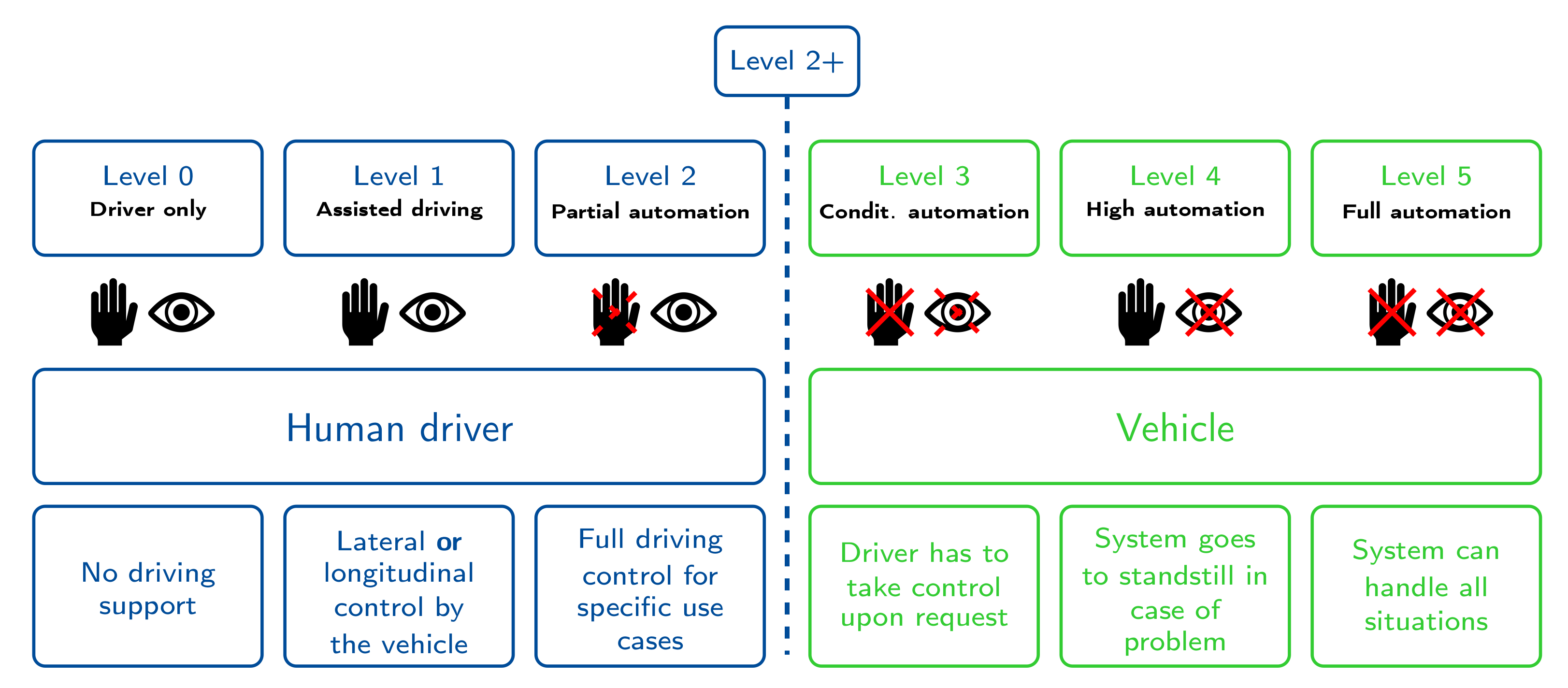
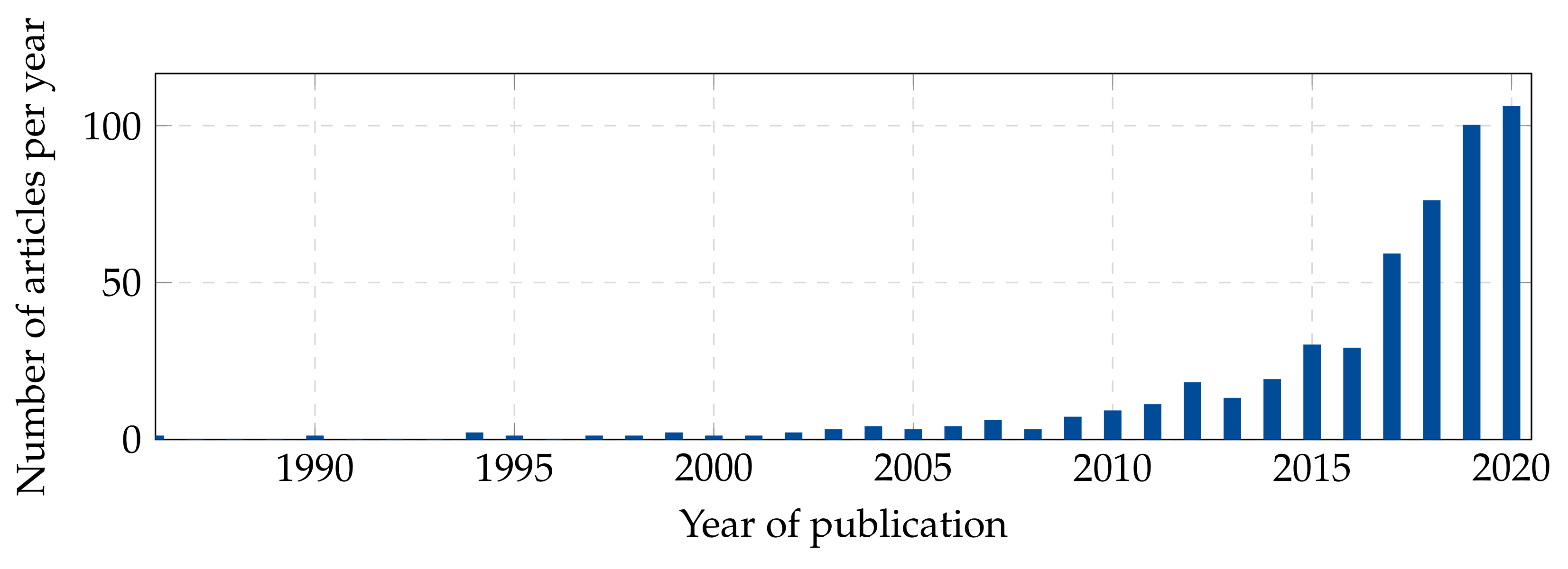
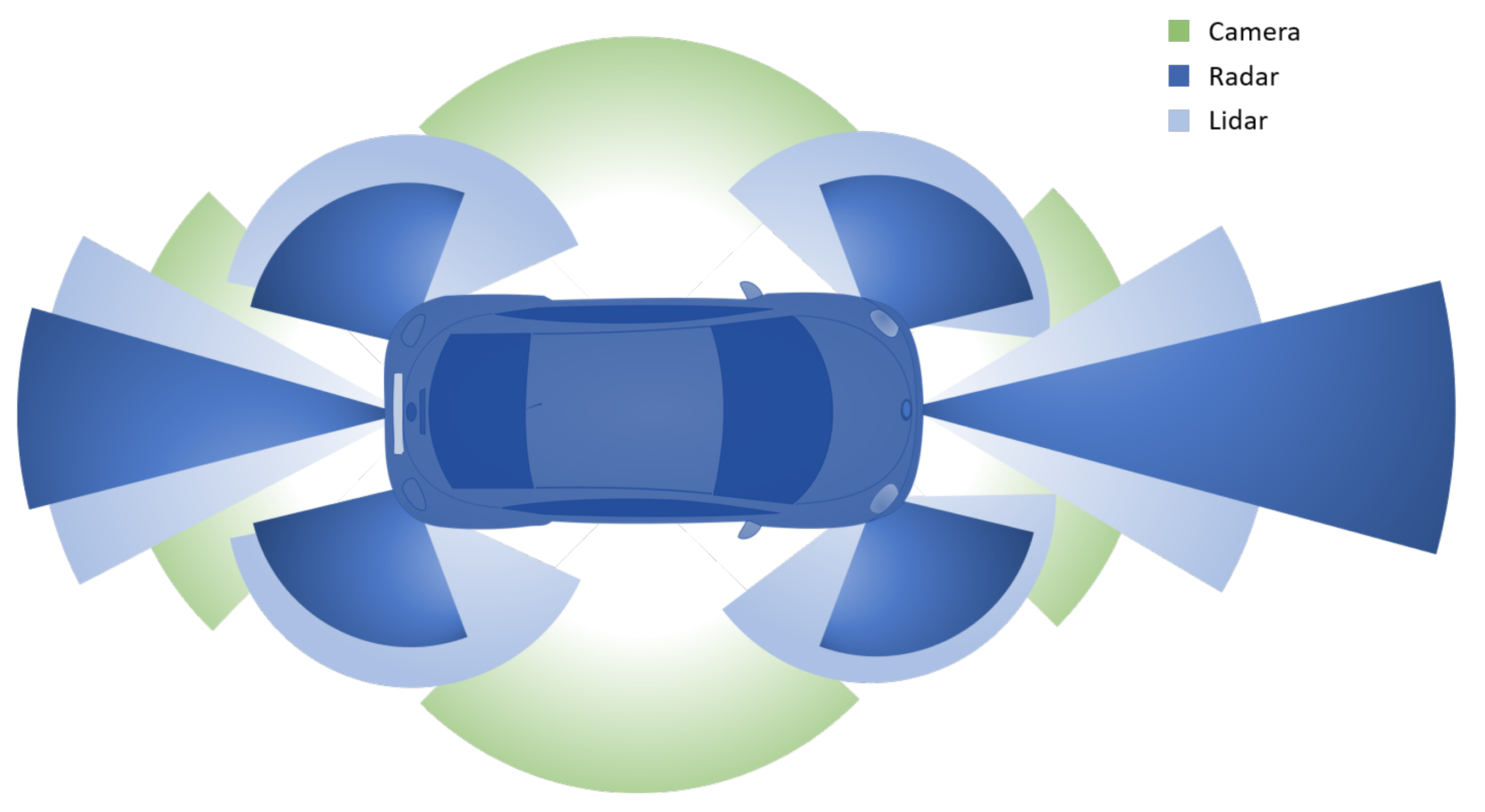
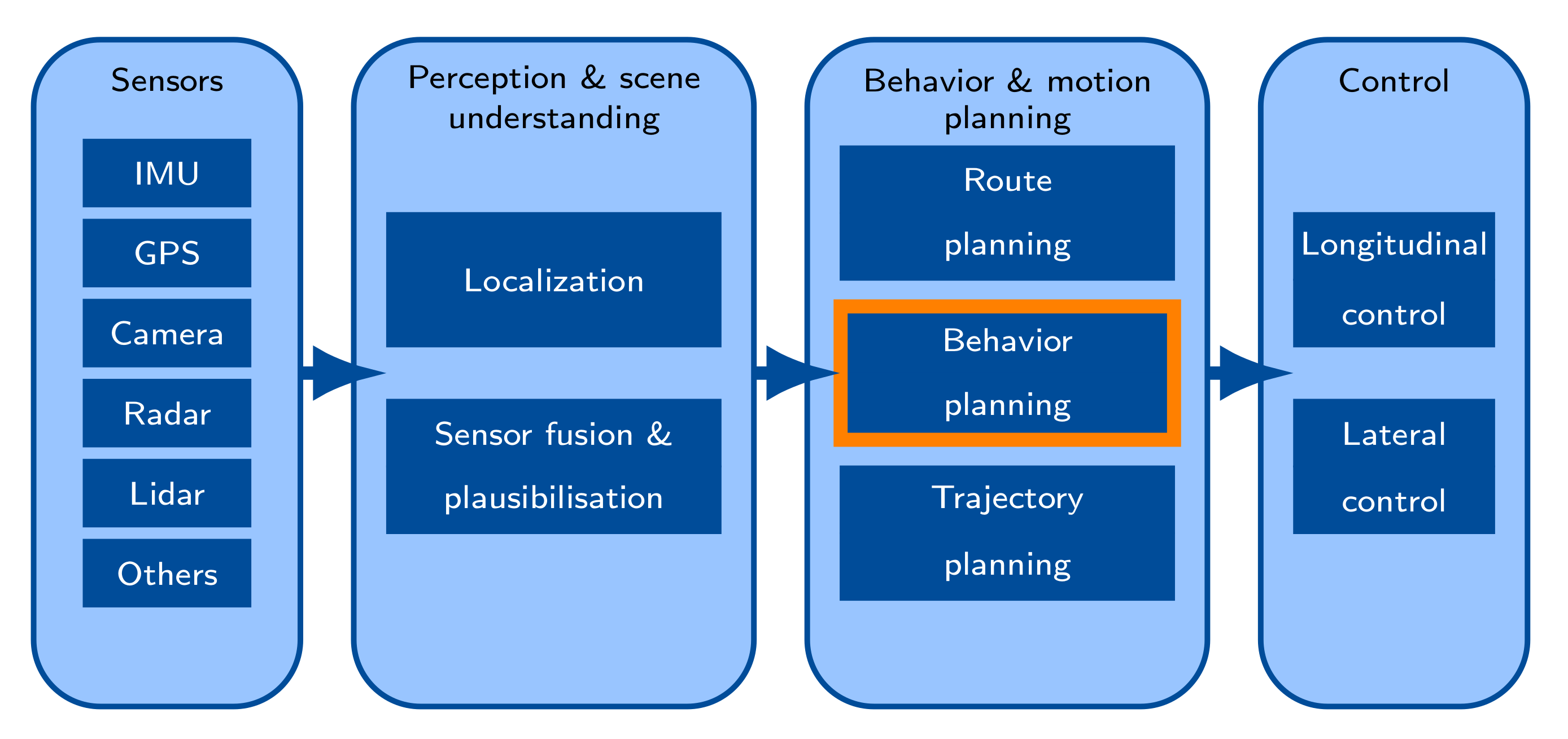
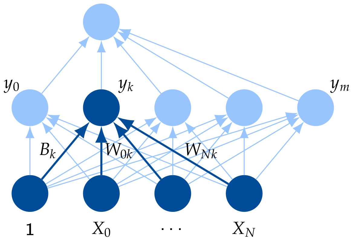
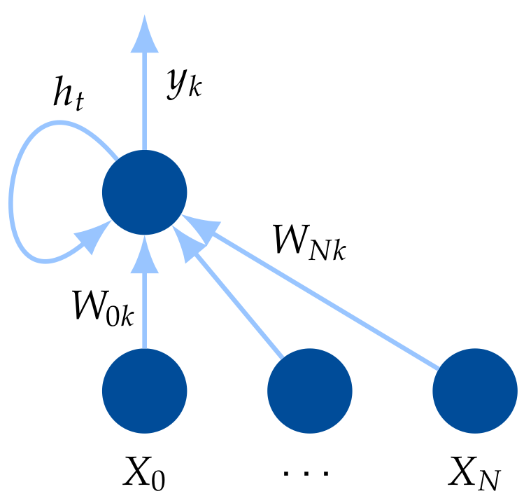
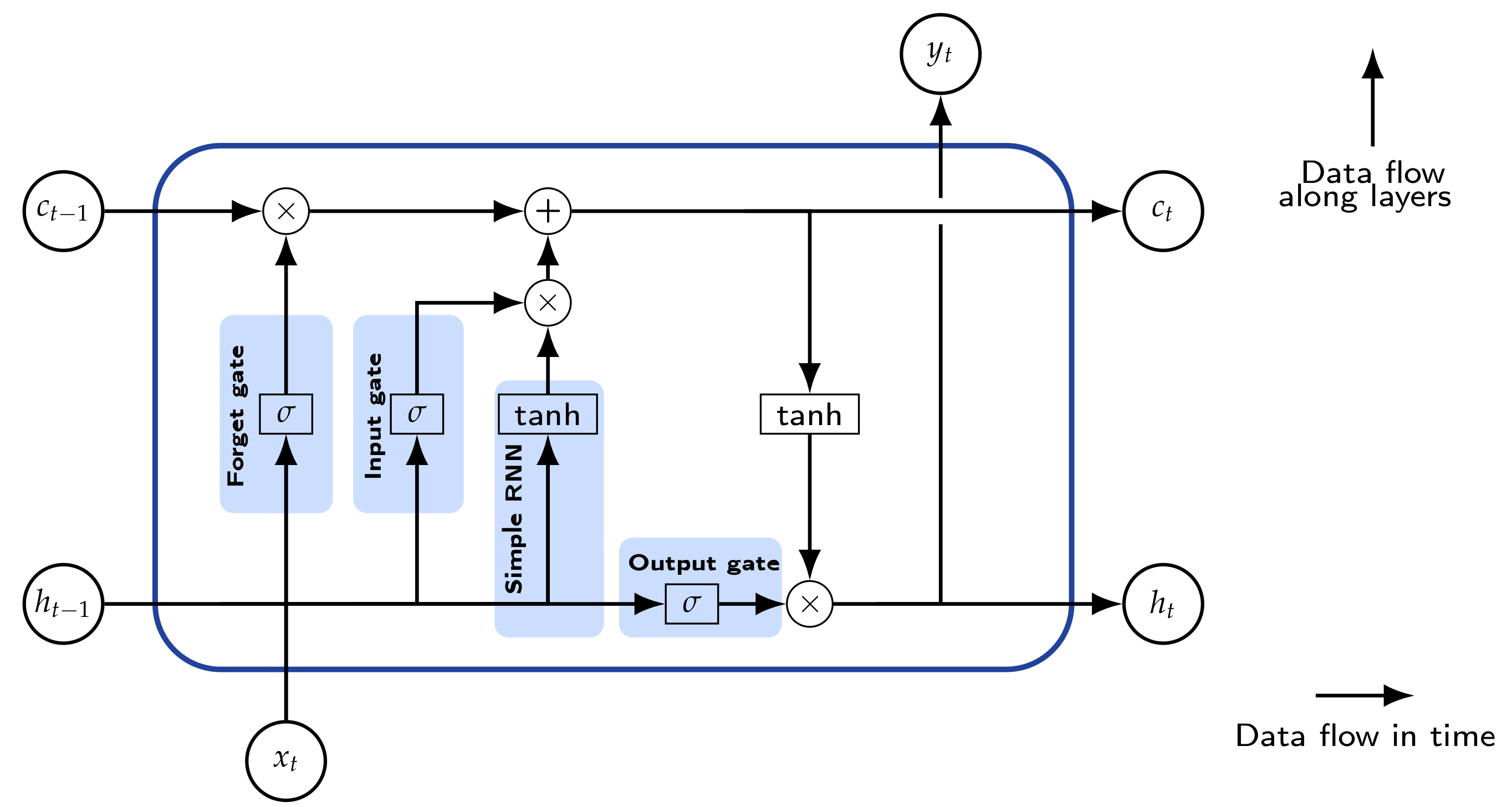
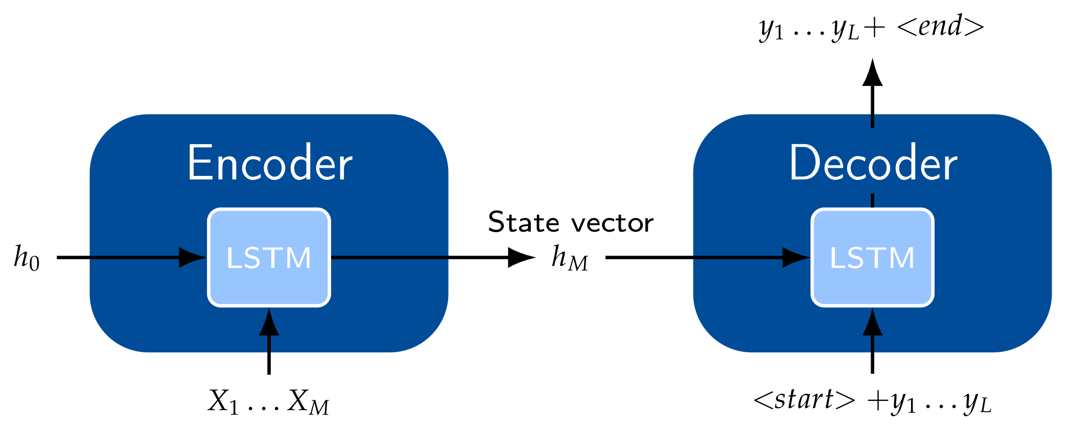
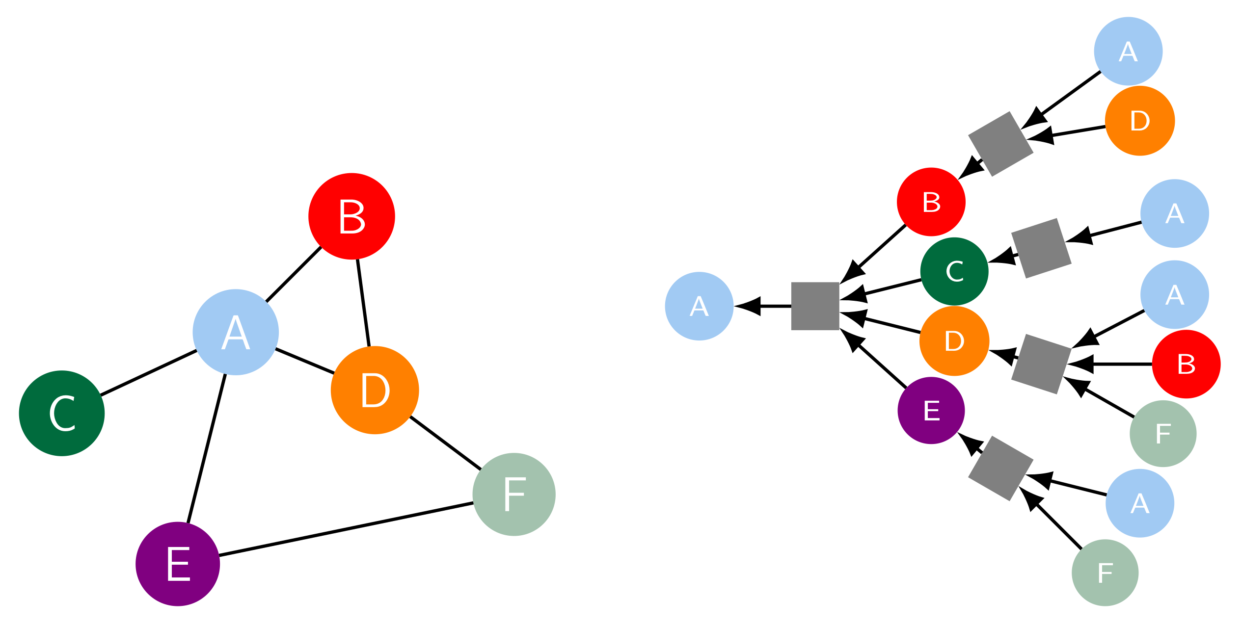
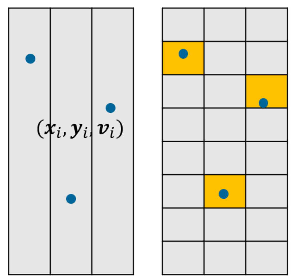
Table 1.
Overview of publications on scene prediction for AD. Neural network models are grouped under “L” (LSTM/GRU), “C” (CNN), “G” (GNN), and “A” (Attention). Some papers are also available at [58]. For the error it is specified the number of modes, K, over which the prediction is sampled, if applicable. See abbreviations list.
| Authors | Data | Year | Method | Horizon [s] | Metrics | Error [m] |
|---|---|---|---|---|---|---|
| Hermes et al. [59] | real | 2009 | Clustering | 3 | RMSE | |
| Houenou et al. [60] | real | 2013 | CYRA | 4 | RMSE | 0.45 |
| Deo et al. [61] | real | 2018 | VGMM | 5 | MAE | 2.18 |
| Casas et al. [62] | real | 2018 | C | 3 | MAE | 1.61 |
| Park et al. [63] | real | 2018 | L | 2 | MAE | 0.93 () |
| Cui et al. [64] | real | 2019 | C | 6 | ADE | 2.31 () |
| Altche et al. [65] | NGSIM | 2017 | L | 10 | RMSE | 0.65 1 |
| Deo et al. [66] | NGSIM | 2018 | L+C | 5 | RMSE | 4.37 |
| Chandra et al. [67] | NGSIM | 2019 | L+C | 5 | ADE/FDE | 5.63/9.91 |
| Zhao et al. [68] | NGSIM | 2019 | L+C | 5 | RMSE | 4.13 |
| Tang et al. [69] | NGSIM | 2019 | G+A | 5 | RMSE | 3.80 () |
| Song et al. [70] | NGSIM | 2020 | L+C | 5 | RMSE | 4.04 |
| Chandra et al. [71] | NGSIM | 2020 | G+L | 5 | ADE/FDE | 0.40/1.08 |
| Lee et al. [72] | KITTI | 2017 | L+C | 4 | RMSE | 2.06 |
| Choi et al. [73] | KITTI | 2020 | G+L+C | 4 | ADE/FDE | 0.75/1.99 () |
| Lee et al. [72] | SDD | 2017 | L+C | 4 | RMSE | 5.33 |
| Chai et al. [74] | SDD | 2019 | C | 5 | ADE | 3.50 () |
| Mangalam et al. [75] | SDD | 2020 | A | 5 | ADE/FDE | 0.18/0.29 () |
| Tang et al. [69] | Argoverse | 2019 | G+A | 3 | ADE | 1.40 () |
| Chandra et al. [71] | Argoverse | 2020 | G+L | 5 | ADE/FDE | 0.99/1.87 |
| Park et al. [76] | Argoverse | 2020 | L+A | 3 | ADE/FDE | 0.73/1.12 () |
| Song et al. [77] | Argoverse | 2021 | L+C+A | 3 | ADE/FDE | 1.22/1.56 () |
| Zeng et al. [78] | Argoverse | 2021 | G+C | 3 | ADE/FDE | 0.9/1.45 () |
| Casas et al. [79] | nuScenes | 2020 | G+C | 3 | RMSE | 1.45 |
| Phan-Minh et al. [80] | nuScenes | 2020 | C | 6 | ADE/FDE | 1.96/9.26 () |
| Liang et al. [81] | nuScenes | 2020 | L+C | 3 | ADE/FDE | 0.65/1.03 |
| Park et al. [76] | nuScenes | 2020 | L+A | 3 | ADE/FDE | 0.64/1.17 () |
| Narayanan et al. [82] | nuScenes | 2021 | C+L | 4 | ADE/FDE | 1.10/1.66 () |
| Casas et al. [79] | ATG4D | 2020 | G+C | 3 | RMSE | 0.96 |
| Liang [81] | ATG4D | 2020 | L+C | 3 | ADE/FDE | 0.68/1.04 |
| Chandra et al. [71] | Lyft | 2020 | G+L | 5 | ADE/FDE | 2.65/2.99 |
| Chandra et al. [71] | Apolloscape | 2020 | G+L | 3 | ADE/FDE | 1.12/2.05 |
| Li et al. [83] | INTERACTION | 2020 | G+C+A | 5 | ADE/FDE | 1.31/3.34 |
| Choi et al. [73] | H3D | 2020 | G+L+C | 4 | ADE/FDE | 0.42/0.96 () |
| Song et al. [70] | HighD | 2020 | L+C | 5 | RMSE | 2.63 |
| Mohta et al. [84] | X17k | 2021 | C | 3 | FDE | 0.85 |
1 Only lateral position considered.
Publisher’s Note: MDPI stays neutral with regard to jurisdictional claims in published maps and institutional affiliations. |
© 2022 by the authors. Licensee MDPI, Basel, Switzerland. This article is an open access article distributed under the terms and conditions of the Creative Commons Attribution (CC BY) license (https://creativecommons.org/licenses/by/4.0/).
Share and Cite
MDPI and ACS Style
Stockem Novo, A.; Krüger, M.; Stolpe, M.; Bertram, T. A Review on Scene Prediction for Automated Driving. Physics 2022, 4, 132-159. https://0-doi-org.brum.beds.ac.uk/10.3390/physics4010011
AMA Style
Stockem Novo A, Krüger M, Stolpe M, Bertram T. A Review on Scene Prediction for Automated Driving. Physics. 2022; 4(1):132-159. https://0-doi-org.brum.beds.ac.uk/10.3390/physics4010011
Chicago/Turabian StyleStockem Novo, Anne, Martin Krüger, Marco Stolpe, and Torsten Bertram. 2022. "A Review on Scene Prediction for Automated Driving" Physics 4, no. 1: 132-159. https://0-doi-org.brum.beds.ac.uk/10.3390/physics4010011