Simulating Three-Wave Interactions and the Resulting Particle Transport Coefficients in a Magnetic Loop


Department of Physics and Astronomy, University of Turku, FI-20014 Turku, Finland
*
Authors to whom correspondence should be addressed.
Physics 2022, 4(2), 394-408; https://0-doi-org.brum.beds.ac.uk/10.3390/physics4020026
Submission received: 10 January 2022
/
Revised: 17 March 2022
/
Accepted: 18 March 2022
/
Published: 31 March 2022
(This article belongs to the Special Issue A Themed Issue in Honor of Professor Reinhard Schlickeiser on the Occasion of His 70th Birthday)
Abstract
:In this paper, the effects of wave–wave interactions of the lowest order, i.e., three-wave interactions, on parallel-propagating Alfvén wave spectra on a closed magnetic field line are considered. The spectra are then used to evaluate the transport parameters of energetic particles in a coronal loop. The wave spectral density is the main variable investigated, and it is modelled using a diffusionless numerical scheme. A model, where high-frequency Alfvén waves are emitted from the two footpoints of the loop and interact with each other as they pass by, is considered. The wave spectrum evolution shows the erosion of wave energy starting from higher frequencies so that the wave mode emitted from the closer footpoint of the loop dominates the wave energy density. Consistent with the cross-helicity state of the waves, the bulk velocity of energetic protons is from the loop footpoints towards the loop apex. Protons can be turbulently trapped in the loop, and Fermi acceleration is possible near the loop apex, as long as the partial pressure of the particles does not exceed that of the resonant waves. The erosion of the Alfvén wave energy density should also lead to the heating of the loop.
1. Introduction
Coronal loops are closed magnetic field structures in the solar atmosphere, filled with dense plasma [1]. They vary greatly in length, ranging from tens to tens of thousands of kilometers, or even further. Loops are important in many regions of the corona, including the active regions where the solar active phenomena, such as flares, are hosted [2].
Non-thermal spectral line broadening, most likely caused by high-frequency Alfvén waves, has been observed in coronal loops; see, e.g., [3,4,5,6], so the transport of these waves in loops is of interest. Under the Wentzel-Kramers-Brillouin (WKB) approximation, a magnetohydrodynamic (MHD) wave propagates in a static background plasma conserving its frequency and refracting under the laws of geometric optics. Alfvén waves have the property that their group velocity is directed along the magnetic field and the refraction of the wave vector is towards the lower values of the Alfvén speed. If the field line is anchored to the solar surface only at one end, all waves injected at the Sun propagate in the same direction along the field, i.e., outward from the Sun. However, in the case of a closed field line, i.e., a loop, both ends of the field line can inject waves into the loop. This leads us to a situation where counter-propagating waves are present. Thus, wave–wave interactions between counter-propagating waves become a topic of investigation to find out how the spectral energy density of the waves is evolving beyond the WKB approximation. Three-wave interactions have been studied theoretically (see, e.g., [7,8,9]), numerically (see, e.g., [10,11,12]), and experimentally (see, e.g., [13,14]). Their descriptions in coronal (see, e.g., [15]), and solar-wind (see, e.g., [16,17]) plasmas, have been a topic of recent research.
MHD wave spectra in magnetized plasmas determine the transport parameters of energetic charged particles [18], which are an important element of solar eruptions such as solar flares and coronal mass ejections; see, e.g., [19,20,21]. Under the weak turbulence approximation, wave–wave interactions can, to the lowest order, be treated as three-wave interactions [22], where two waves either coalesce to produce a single wave or a single wave decays to produce two waves.
In this paper, the effect of three-wave interactions on Alfvén waves propagating in coronal loops is considered. The influence of these on the wave spectra is studied, and the spectra to compute the transport parameters of energetic particles in these loops is used. The modification of the spectra by the three-wave interactions are discussed, and the consequences of the resulting spectra on particle transport inside the loops are considered. It is shown that under plausible assumptions of injected wave spectral energy densities, three-wave interactions lead to a significant modification of wave spectra and the mode of particle transport inside the loop. The study concludes that wave–wave interactions in coronal plasmas should be considered when the coupled evolution of waves and particles is modelled.
2. Theory
To investigate the three-wave interactions of two Alfvén waves and a magnetosonic wave, the model of Chin and Wentzel [22,23] is used which has been extended, e.g., by Zhao et al. [24] and Modi and Sharma [25], and applied to the case of two Alfvén waves and a sound wave by Vainio and Spanier [26] to calculate the cross-helicity of Alfvén waves downstream of a fast-mode shock. Only the low-plasma- regime, where the Alfvén speed is larger than the sound speed, a condition applicable to most of the corona and inner solar wind [27], is studied. For simplicity, the study is limited to the discussion of waves propagating parallel and anti-parallel to the magnetic field. Eigenmodes propagating along the mean magnetic field are circularly polarized and the conservation of angular momentum is equivalent to conservation of polarization in three-wave interactions [28]. In the non-dispersive limit, the same evolution equation applies to both left-handed and right-handed waves. When computing the particle transport coefficients, it is assumed that both circular polarization states have the same intensity, which would be the case for linearly polarized waves. The three-wave interactions applicable to such conditions are an Alfvén wave decaying into a sound wave and a counter-propagating Alfvén wave, or the coalescence of an Alfvén wave and a sound wave into an Alfvén wave, i.e.,
where A and denote Alfvén waves, S denotes sound waves, and the + (−) sign denotes a wave propagating parallel (anti-parallel) to the magnetic field. The three-wave interaction requires the resonance conditions,
to be met, where is the wave angular frequency, k is the wave number, and are the dispersion relations of the waves (applicable to the primed ones, as well), is the Alfvén speed, is the sound speed, B is the magnetic field magnitude, is the mass density, P is the thermal pressure, and is the adiabatic index of the plasma. In the convention used, and the sign of k denotes the propagation direction of the wave. Using the resonance conditions and dispersion relations, one can solve the wave numbers and frequencies of the decay products. In particular, for the Alfvén waves
where primed (unprimed) quantities are for waves on the right-hand (left-hand) side of Equation (1).
The model considered uses the simplified coronal loop presented in Figure 1 to eliminate the effects of field-line geometry on the wave distribution. In particular, it is assumed that the wave speeds remain constant over the whole length of the loop and that the loop has an Alfvén speed lower than its surroundings to allow waves to be ducted and maintain their wavevector as parallel/anti-parallel to the field. Additionally, gravitational stratification is neglected to have a constant density and temperature along the loop length.
Finally, sound waves in a coronal plasma are assumed to quickly damp by thermal particles, leading to only the reactions proceeding from left to right in Equation (1) being relevant. This simplifies the three-wave interaction term in the wave evolution equation so that all terms proportional to sound-wave intensity vanish. Thus, the equations governing the evolution of the Alfvén waves are [26]
where
are the normalized spectral energy densities of the Alfvén waves propagating parallel (+) and anti-parallel (−) to the field, are the wave frequencies in the respective directions, are the wave action densities in the respective directions, and is the background magnetic field energy density. Here, the left-hand side implements the spatial transport of wave-energy density along the magnetic field and the right-hand side the evolution of wave-energy densities due to wave–wave interactions. The net growth rates due to three-wave interactions are given as [26]
The rate is dependent only on the energy density of the counter-propagating wave mode. In particular, the term describes counter-propagating waves from angular frequency decaying into waves at angular frequency and those, in turn, decaying into counter-propagating waves at . The frequency domain under consideration extends to proton cyclotron frequency only, since dispersive effects [7,8,28] are not considered in the model.
Wave–particle interactions between energetic charged particles and MHD waves can be described as a resonant elastic scattering of particles in the frame co-moving with the waves [29,30,31]. In a homogeneous mean magnetic field, when scattering is strong enough to keep the particle distribution close to isotropic, the spatial transport of particles is a diffusion–advection process, where the advection velocity is determined by the mean velocity of the waves and the diffusion coefficient is determined by the rate of scattering. In addition, adiabatic particle energy changes result from gradients of the advection velocity and stochastic acceleration from counter-propagating waves scattering particles in the same volume [18,29]. To analyze the effect of the Alfvén waves on charged particles, here, the transport equations are used, as derived by Schlickeiser [18]:
where is the pitch-angle averaged distribution function of the energetic particles, p and v are the particle momentum and speed, is the spatial diffusion coefficient, is the coefficient of advection and adiabatic cooling, is the coefficient of momentum diffusion, and is the particle source. In the integrals, is the cosine of pitch angle and , , and are the Fokker–Planck coefficients related to momentum-space diffusion produced by wave–particle interactions [18]. For the normalized wave energy density, , they have the following forms:
where
is the wave frequency of parallel/anti-parallel (+/−) propagating waves resonant with particles of speed v and pitch-angle cosine and is the (relativistic) particle cyclotron frequency.
Because of the use of MHD dispersion relations, only ion transport can be considered. Additionally, since the discussion is limited to the frequency range below the ion-cyclotron frequency, one needs to deal with the resonance gap resulting from the cut-off in the spectrum. This is achieved by extrapolating the spectra with a spectral index of from the last frequency considered below the cyclotron frequency, where is defined as
and is the spectral index () solved from the last two cells below the cyclotron frequency. This produces Fokker–Planck coefficients that are approximately consistent with ion-cyclotron waves, with the same spectral index in wavenumber as the highest-frequency Alfvén waves, being responsible for scattering across the gap [32].
3. Numerical Methods
The wave evolution equations are solved on a two-dimensional grid as a function of time. The waves are transported in the spatial dimension using a diffusionless scheme, where wave spectral energy densities are propagated by one grid-cell of size per each time step, . Thus, as the Alfvén speed is constant in the presented model, the time step is defined as
In the angular frequency direction, a logarithmic grid spacing with the last cell being equal to the proton cyclotron frequency is employed. Solving the rest of the cells from there onwards:
where N denotes the last cell of the grid and . The lowest frequency on the grid is set to a sufficiently low value to prevent boundary effects from altering the results of the simulation.
Operator splitting is used so that the spatial transport half-cycle is followed by a half-cycle implementing the wave–wave interactions in a time-explicit scheme. Thus, the approximate solution to the evolution Equation (4) can be written as a single step as
Waves are injected from both ends of the spatial domain and those incident on the spatial boundaries from inside the domain are absorbed. The boundary values for the frequency domain are determined as follows: The lower boundary condition is set as
The upper boundary is set by assuming that cyclotron waves are damped by thermal plasma ions at the lowest wavelengths. That is,
is taken.
The parameters used in the simulations are chosen from ranges provided by [33] for the magnetic field strength and [1] for the rest:
from which one can solve for the cyclotron frequency used as the upper boundary for the angular frequency axis,
where e and are the charge and mass of a proton.
The wave spectra injected at the spatial boundaries are formulated so that the spectrum is flat at low frequencies, below , and obeys a power-law with a spectral index of thereafter. The spectrum is also set to equal zero at the cyclotron frequency to synergize with the frequency boundary condition. The resulting form is
where is a normalization value. Here, is used throughout the study.
Additionally, the injection spectrum contains a temporal ramp to provide a gradual increase in the wave spectral energy densities. The simulation reaches the steady-state injection after the time . Thereafter, once a full wave-transport time has passed (), a steady state emerges.
Thus, the injection spectrum for the wave mode propagating in the positive x direction is of the form
where is a parameter that controls the duration of the ramping up of the injection and the Heaviside step function. The injection of the wave mode propagating in the negative x direction is identical, except that it is set at the other boundary, .
The assumption of broadband wave emission is not based on a particular physical model of Alfvén wave generation in the footpoints of the coronal loop. To note, however, is that similar modelling has been applied, e.g., in connection with cyclotron heating on open field lines; see, e.g., [34,35]. Additionally, the observed heliospheric turbulence evolution suggests a broadband power spectrum of the form , identical to those considered here at low frequencies, being eroded by turbulent processes (see, e.g., [36]). The heliospheric fluctuations are, of course, observed at lower frequencies but the spectrum below the correlation scale still spans several orders of magnitude. Thus, we regard the assumption of broadband wave emission from the footpoints of the loop as a reasonable, albeit not the only possible, assumption.
4. Results
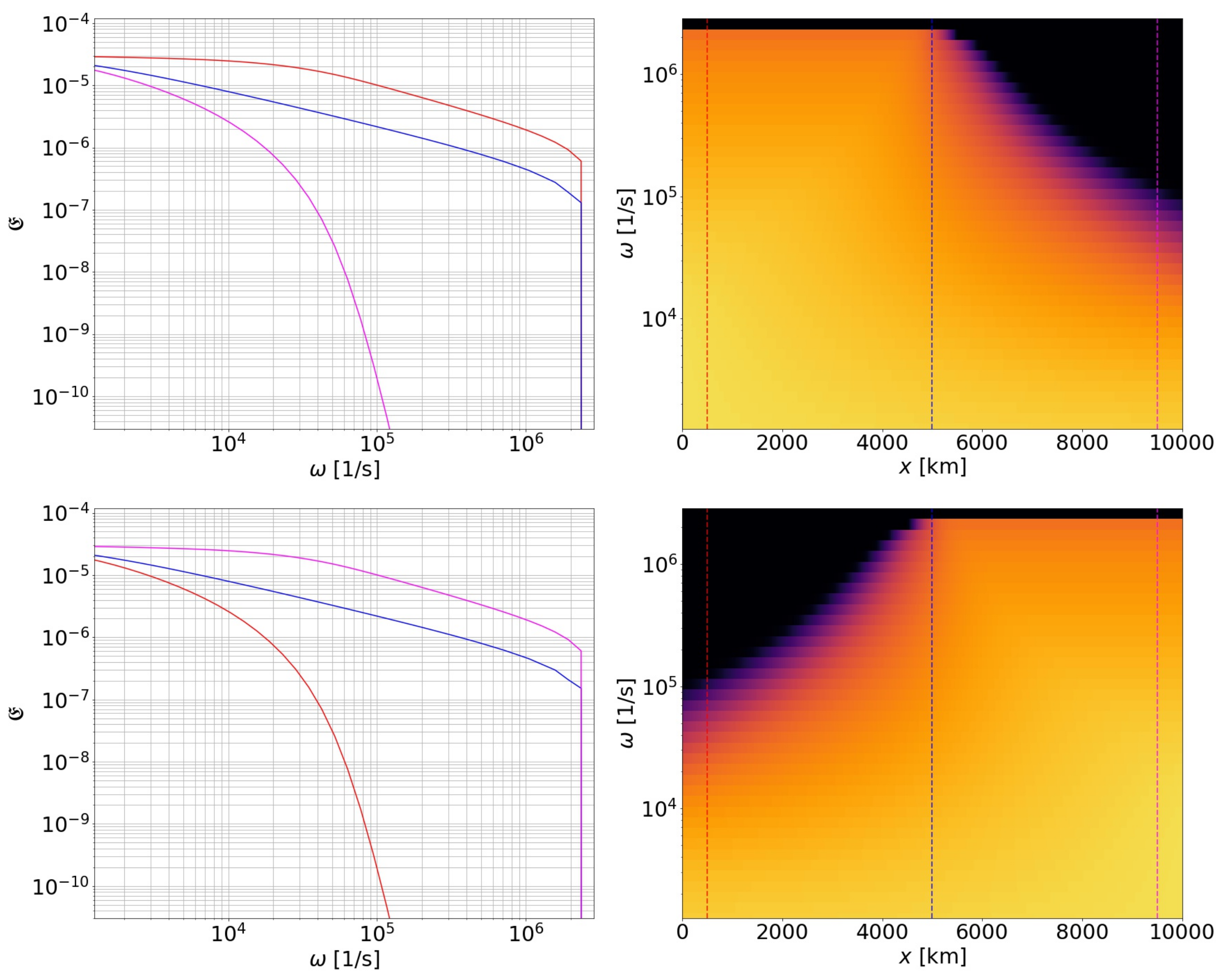
The results on wave spectra are presented as a set of contour plots depicting the wave spectral energy density in x and , and plots of as a function of the wave frequency from three locations in the simulation box. The angular frequency range to be investigated was chosen to correspond to wavelengths above 10 km, and up to the proton cyclotron frequency. Figure 2 presents the spectra with a normalization value of . One can see the three-wave interactions having the largest effect at high frequencies. The wave spectra evolve so that the wave modes propagating away from the closer end of the loop (the surface of the Sun) dominate. In the centre of the loop, both wave spectra are equal, as required by symmetry.
To compute the Fokker–Planck coefficients, the value of is logarithmically interpolated from the simulation data at the resonant frequency . At values of close to , the resonant frequency falls outside the grid, producing the well-known resonance gap. In this study, it is assumed that processes such as wave dispersion [32] and/or resonance broadening [37] fill the gap and prevent the integrals of the Fokker–Planck coefficients from diverging. In particular, the gap is filled by extrapolating the spectral energy density values from the last simulated frequency value on the grid () to the region above that resonant frequency, as if scattering in the resonance gap would be caused by ion-cyclotron waves with a wavenumber spectrum extrapolated from the Alfvénic range to the ion-cyclotron range (see Section 2 above).
Let us consider protons with speeds . The calculations are non-relativistic, in line with (with c being the speed of light) applicable for the parameters studied in this paper.
The bulk velocity of the energetic particles is derived using Equations (6) and (8). If only the leading order dependence of on momentum () is accounted for, the bulk velocity of energetic protons becomes
The integral is evaluated from the Fokker–Planck coefficients using the trapezoidal rule.
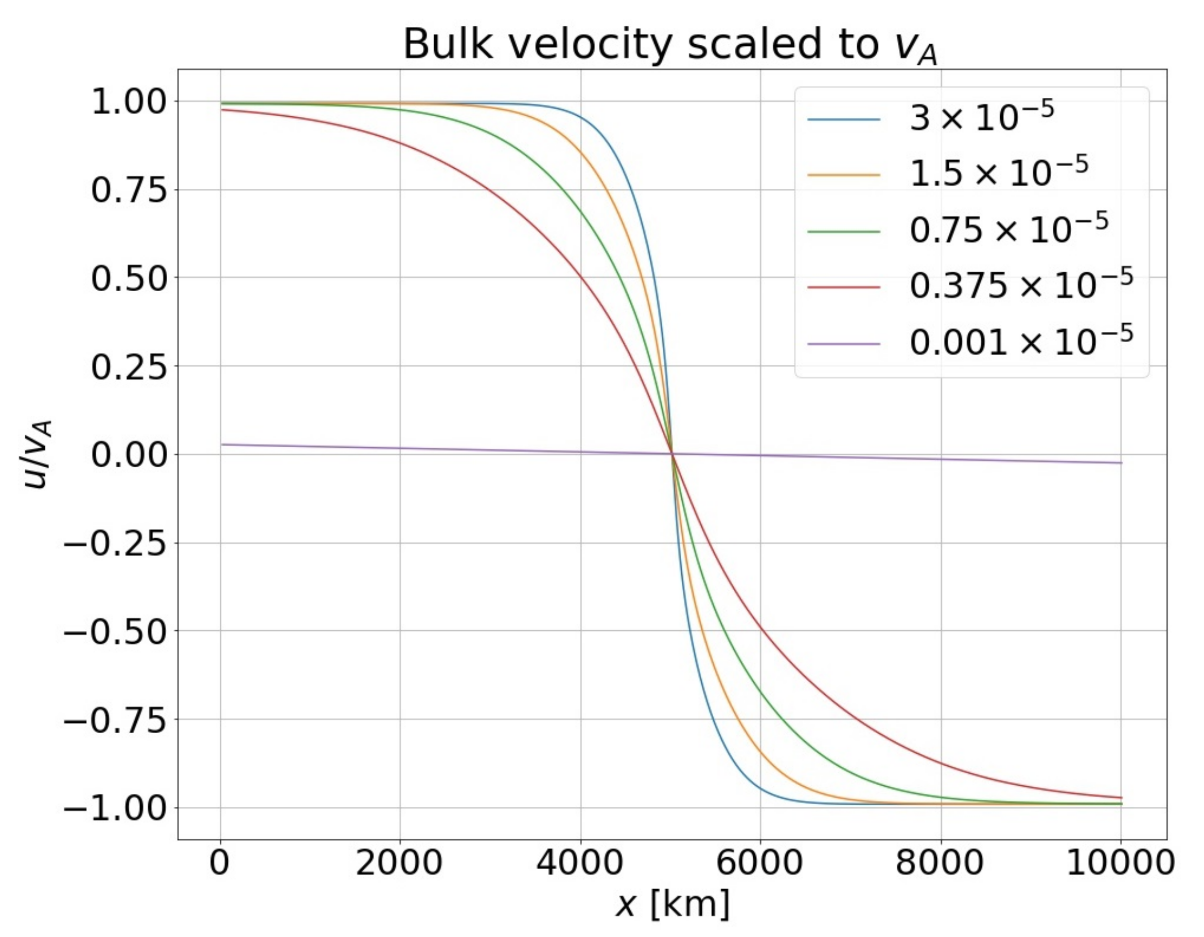
The results for simulations with different normalization values can be seen in Figure 3. In higher injection spectral energy density simulations, particles move away from the surface of the Sun at the Alfvén velocity in almost all of the spatial domain. With lower energy densities, the region in the middle of the loop with a lower bulk speed broadens. The bulk speed approaches zero as the injection spectral energy density vanishes, as expected for non-interacting waves injected at equal intensities from both ends of the loop.
Next, spatial diffusion is considered. The scattering mean free path for the particles is derived using Equation (7) as
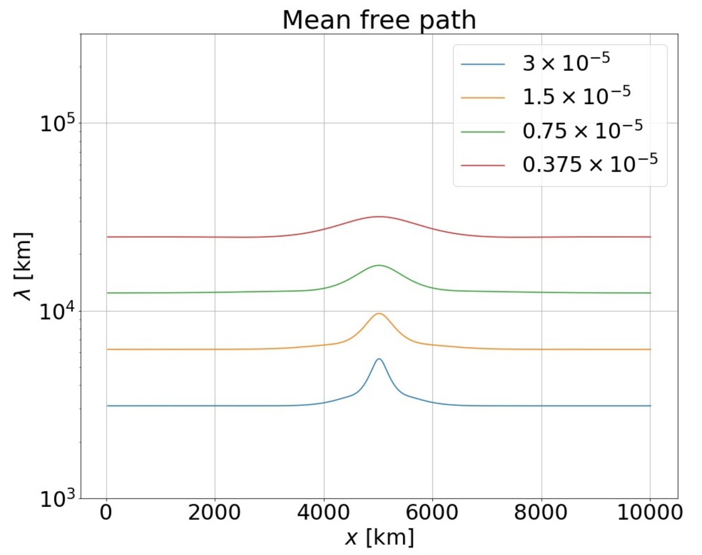
The mean free paths of simulations with different spectral energy densities are presented in Figure 4. In the two lowest presented wave spectral energy densities, mean free paths exceed the loop size, but in the two higher spectral energy densities, the mean free paths are smaller than the loop length. This allows the particles to be efficiently isotropized in the loop, a requirement for the diffusion approximation employed in the transport equation to be valid.
The actual mode of transport of particles inside the loop is determined by the diffusion length, and the length scale particles can diffuse upstream in a flow. For a constant spatial diffusion coefficient and bulk speed (and neglecting momentum diffusion), the transport equation reads
and can be solved as
where A and B are constants to be determined by boundary conditions. One can see that the diffusion length, , is the scale height of the distribution. Thus, a loop with a size certainly larger than the diffusion length can turbulently trap particles with a converging flow of the scattering centres towards the loop apex.
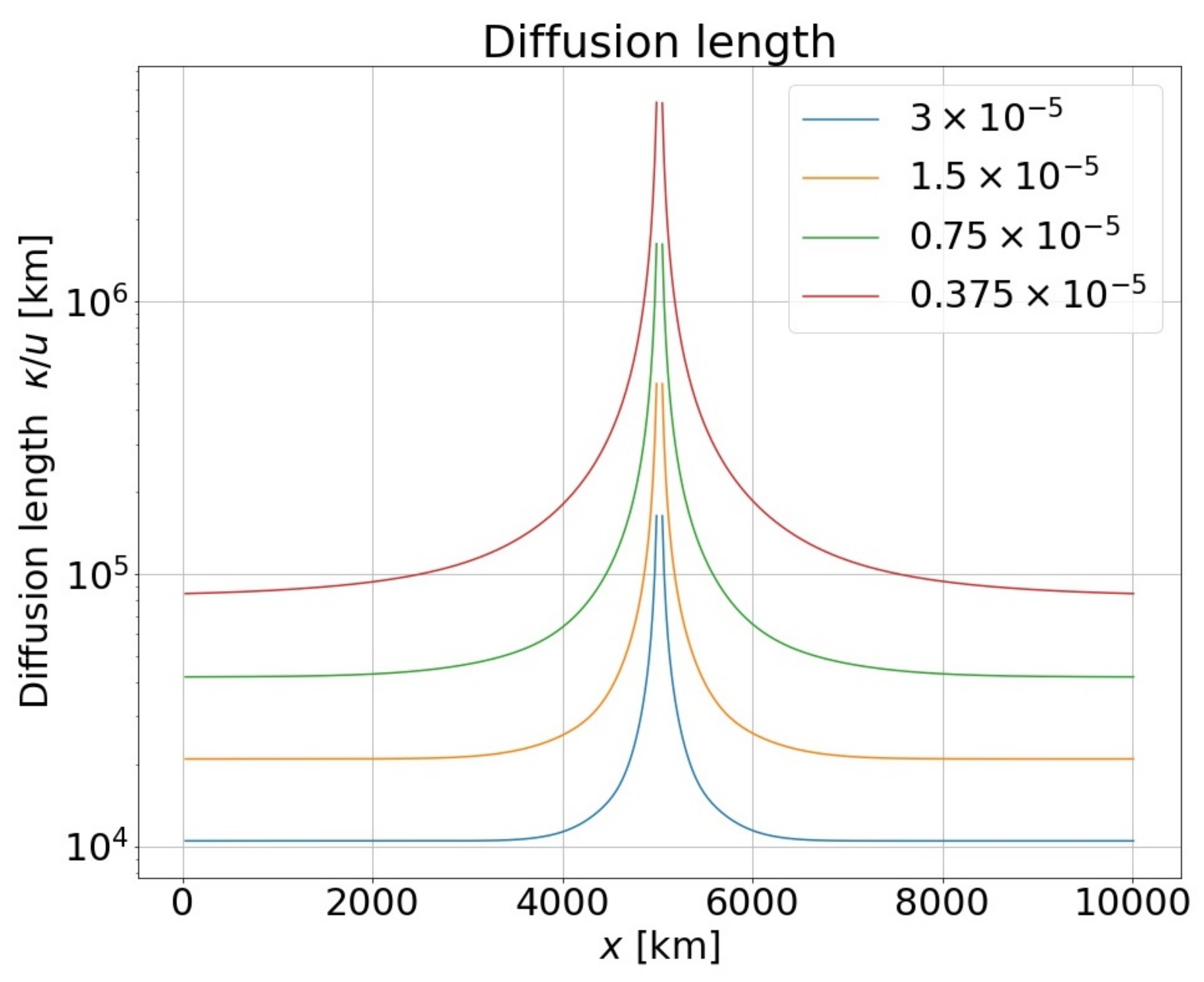
The diffusion lengths of different wave spectral energy density simulations are presented in Figure 5. As the diffusion length diverges in the middle of the loop (since there), the diverging part is cut off in the figure. The diffusion length exceeds the loop length in all injection cases considered, leading to the conclusion that with these wave spectral energy densities the particles would not be confined in the loop but would be able to diffuse out of it quite efficiently.
In order to study this further, longer loops were then investigated. In Figure 6, a 30,000 km loop with a lower injection spectral energy density is presented and compared with the 10,000 km loop with a higher injection spectral energy density presented in Figure 2. An interesting result is the invariant nature of the product between the wave spectral energy density and the loop length: scaling the injected wave spectral energy inversely with the loop length produces identical-shaped wave spectral energy densities in a scaled spatial coordinate and frequency, i.e., in steady state,
where is the dimensionless spatial coordinate scaled to the length of the loop. This can be seen to hold also by applying these scaling laws to the wave transport Equations (4) and assuming a steady state.
To investigate the evolution of the particle transport properties, analyses of the bulk velocity, mean free path, and diffusion length were conducted on the 30,000 km loop with injection normalization parameters and to the 10,000 km loop with identical injections. The results are presented in Figure 7, Figure 8, Figure 9 and Figure 10, where the particle transport coefficients are plotted along the dimensionless spatial coordinate . The curves, representing the spectra, given in Figure 2 and Figure 6, lie on top of each other, as expected. The other cases are ordered so that the higher injection spectral energy density corresponds to the steeper gradient of the bulk speed. The case with a longer loop and higher spectral energy density of the waves now demonstrates a regime where the loop length exceeds the diffusion length and the turbulent trapping of protons in the loop apex seems plausible.
For these cases, where the bulk velocity is directed towards the loop apex and particles can be confined there diffusively, the model predicts an interesting situation, where first-order Fermi acceleration operates in the loop apex. The requirement of the diffusion length being longer than the gradient scale of the velocity while being shorter than the two “upstream regions” is a shock-like situation where particles can scatter back and forth from converging scattering centres and gain energy while being confined. The particle acceleration time scale in diffusive shock acceleration is [38]
where and are the upstream (downstream) diffusion coefficient and bulk speed and . Applying the analogy of the setup to diffusive shock acceleration, i.e., replacing , and , one can express the first-order Fermi acceleration time scale as
which for the considered case of , km/s and km gives about s.
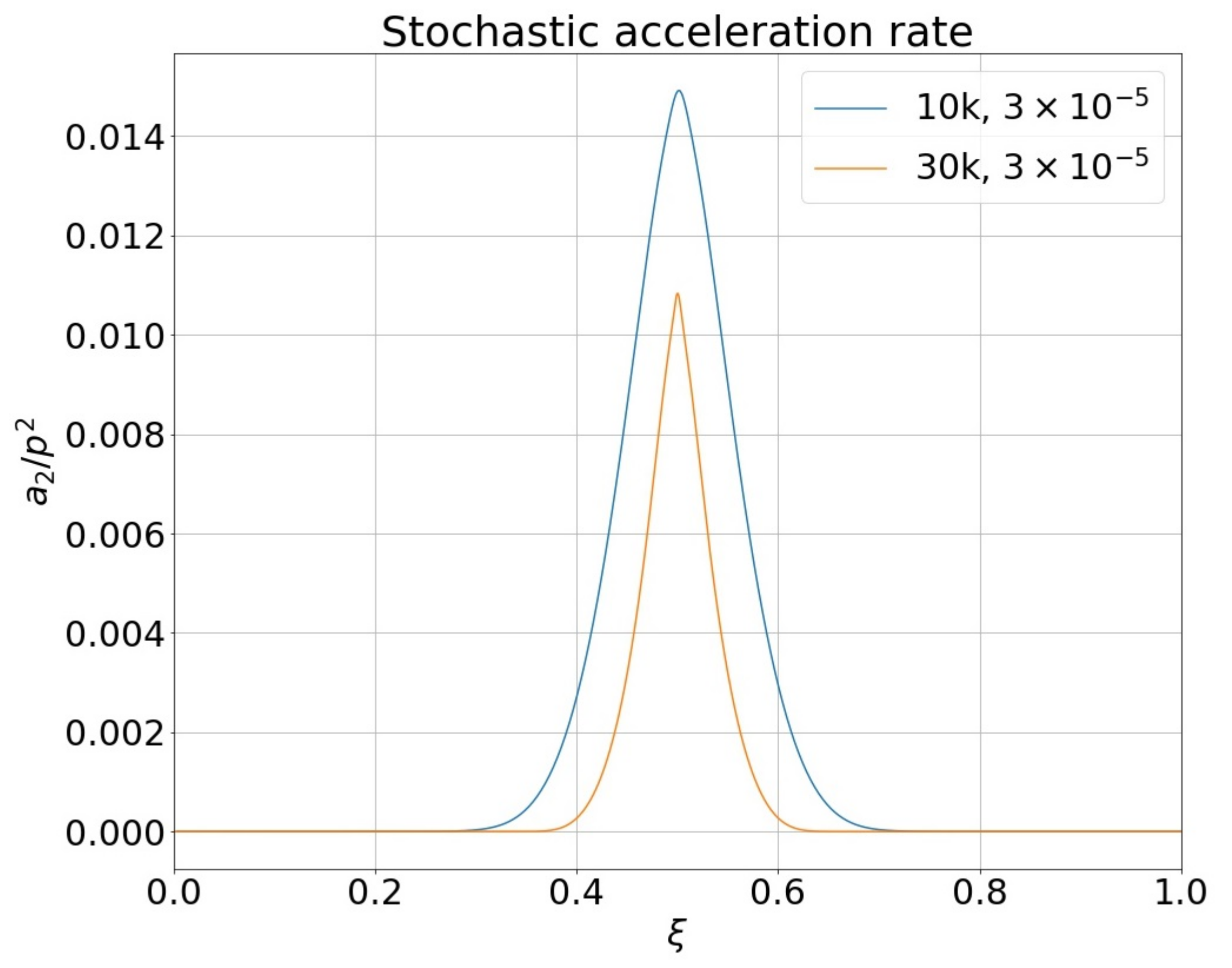
The loop apex is also a potential location for second-order Fermi acceleration, as waves propagating in both directions along the field are present there. Thus, the rate of stochastic acceleration of particles (Figure 10) is also investigated. Let us define it using the coefficient of momentum diffusion (Equation (9)), as , where p is the particle momentum i.e., is the time scale needed for the particles to diffuse a “distance” p in momentum space. The values for the second-order Fermi acceleration rate displayed in Figure 10 are visibly lower than the rate of the first-order Fermi acceleration, s.
5. Discussion and Conclusions
Above, wave transport in a coronal magnetic loop was considered including the effect of three-wave interactions between the counter-propagating Alfvén waves. For wave energy densities still in the weak-turbulence regime (i.e., with values of far lower than unity), it was demonstrated that the interaction of counter-propagating waves erodes the spectrum of the wave mode emitted from the larger distance and leaves the wave field dominated by waves emitted from the closer footpoint. The spectrum erodes in particular at high frequencies. Additionally, the compatibility of the wave amplitudes of the simulation to spectral observations of nonthermal velocities in active regions is investigated. The Alfvén wave amplitude fulfills [39]
where is the amplitude of the velocity fluctuations and is the amplitude of the magnetic field fluctuations. On the other hand, one can write:
due to the definition of as the energy density of the waves (per or , equivalently) divided by the magnetic field energy density. Using an Alfvén wave amplitude of 30 km/s from nonthermal velocity measurements [40] and the Alfvén speed of 2000 km/s from the simulation parameters used, one obtains as an upper limit consistent with observations. Estimating the integral (29) throughout the simulation box for the highest injection value case of and L = 30,000 km gives , showing that the highest values of used in the presented simulations are still comfortably below the limit set by the observations.
One of the major simplifications in the modelling here was the restriction to parallel-propagating waves. If this simplifying assumption is dropped, wave–wave interactions will lead to the development of the spectrum in the perpendicular direction, which may take over the parallel evolution modelled in our study [41]. Wave transport processes such as ducting [42] could allow for the parallel nature of the high frequency Alfvén waves to be maintained, but further studies should be performed to identify the parameters of the coronal loops that could sustain the parallel evolution of the three-wave interactions. Wave–particle interaction processes that produce the highest growth rates for the field-aligned wave modes could also lead to parallel waves dominating but such systems would naturally have more complicated wave transport than this simplified model, where the waves are generated in the loop legs.
In the present study, loops of intermediate lengths were considered corresponding to scales applicable to active regions [1]. It was shown that wave–wave interactions can lead to wave distributions that yield very interesting parameters for charged-particle transport: (1) The bulk velocity of ions interacting with the Alfvén waves is generally directed from the loop legs to the loop apex and is close to the Alfvén speed for most part of the loop if the wave spectral energy density injected into the loop exceeds a threshold value. (2) The diffusion length of energetic (∼MeV) protons can be shorter than the loop length, allowing particles to be turbulently trapped in the loop. (3) The converging velocity of the scattering centres can make the loop apex act as a Fermi acceleration site; the first-order acceleration process seems to dominate over the second-order process, at least with the parameters studied in the modelling here.
However, to point out is that no back-reaction effects of the accelerated particles on the waves were considered in our brief analysis [43,44]. If the accelerated particle pressure greatly exceeds the resonant wave pressure (half of the wave spectral energy density for Alfvén waves), particles streaming away from the acceleration site at the loop apex would actually dampen the waves propagating towards the apex and amplify the waves that propagate towards the footpoints of the loop [43]. Thus, the theory presented here only applies in situations where the externally driven waves are strong enough that their pressure exceeds the partial pressure of the accelerated particles resonant with them. This implies that a full model with all weak-turbulence effects (wave–wave and wave–particle interactions) included would have a natural way of quenching the Fermi acceleration mechanism at the apex.
Let us also point out that as the model predicts the erosion of Alfvén wave spectra by the emission and subsequent absorption of sound waves by the thermal plasma, it leads to the heating of the loop, which might seed the acceleration process with particles from the thermal tail. This is, however, to be a subject of further investigations.
Author Contributions
Conceptualization, R.V.; methodology, S.N. and R.V.; software, S.N.; validation: S.N.; formal analysis, S.N. and R.V.; investigation, S.N. and R.V.; resources, R.V.; data curation, S.N.; writing—original draft preparation, S.N. and R.V.; writing—review and editing, S.N.; visualization, S.N.; supervision, R.V.; project administration, R.V.; funding acquisition, R.V. All authors have read and agreed to the published version of the manuscript.
Funding
This research was funded by the European Union’s Horizon 2020 Programme grant number 870405 (EUHFORIA 2.0).
Data Availability Statement
Not applicable.
Acknowledgments
The authors acknowledge fruitful discussions with A. Afanasiev. This study was performed in the framework of Finnish Centre of Excellence in Research of Sustainable Space (FORESAIL, 2018–2025).
Conflicts of Interest
The authors declare no conflict of interest.
References
- Reale, F. Coronal loops: Observations and modeling of confined plasma. Living Rev. Sol. Phys. 2010, 7, 5. [Google Scholar] [CrossRef] [Green Version]
- Aschwanden, M.J. Physics of the Solar Corona. An Introduction with Problems and Solutions; Springer: Berlin/Heidelberg, Germany, 2005. [Google Scholar] [CrossRef]
- Tian, H.; McIntosh, S.W.; De Pontieu, B.; Martinez-Sykora, J.; Sechler, M.; Wang, X. Two components of the coronal emission revealed by EUV spectroscopic observations. Astrophys. J. 2011, 738, 18. [Google Scholar] [CrossRef] [Green Version]
- Tian, H.; McIntosh, S.W.; Wang, T.; Ofman, L.; De Pontieu, B.; Innes, D.E.; Peter, H. Persistent doppler shift oscillations observed with hinode/eis in the solar corona: Spectroscopic signatures of alfvénic waves and recurring upflows. Astrophys. J. 2012, 759, 144. [Google Scholar] [CrossRef] [Green Version]
- Tian, H.; McIntosh, S.W.; Xia, L.; He, J.; Wang, X. What can we learn about solar coronal mass ejections, coronal dimmings, and Extreme-Ultraviolet jets through spectroscopic observations? Astrophys. J. 2012, 748, 106. [Google Scholar] [CrossRef]
- McIntosh, S.W. The inconvenient truth about coronal dimmings. Astrophys. J. 2009, 693, 1306–1309. [Google Scholar] [CrossRef] [Green Version]
- Shi, Y.; Qin, H.; Fisch, N.J. Three-wave scattering in magnetized plasmas: From cold fluid to quantized Lagrangian. Phys. Rev. E 2017, 96, 023204. [Google Scholar] [CrossRef] [Green Version]
- Shi, Y. Three-wave interactions in magnetized warm-fluid plasmas: General theory with evaluable coupling coefficient. Phys. Rev. E 2019, 99, 063212. [Google Scholar] [CrossRef] [Green Version]
- TenBarge, J.M.; Ripperda, B.; Chernoglazov, A.; Bhattacharjee, A.; Mahlmann, J.F.; Most, E.R.; Juno, J.; Yuan, Y.; Philippov, A.A. Weak Alfvénic turbulence in relativistic plasmas. Part 1. Dynamical equations and basic dynamics of interacting resonant triads. J. Plasma Phys. 2021, 87, 905870614. [Google Scholar] [CrossRef]
- Matteini, L.; Landi, S.; Velli, M.; Hellinger, P. Kinetics of parametric instabilities of Alfvén waves: Evolution of ion distribution functions. J. Geophys. Res. Space Phys. 2010, 115, A09106. [Google Scholar] [CrossRef] [Green Version]
- Matteini, L.; Landi, S.; Zanna, L.D.; Velli, M.; Hellinger, P. Parametric decay of linearly polarized shear Alfvén waves in oblique propagation: One and two-dimensional hybrid simulations. Geophys. Res. Lett. 2010, 37, L20101. [Google Scholar] [CrossRef] [Green Version]
- Chang, O.; Gary, S.P.; Wang, J. Energy dissipation by whistler turbulence: Three-dimensional particle-in-cell simulations. J. Plasma Phys. 2014, 21, 052305. [Google Scholar] [CrossRef] [Green Version]
- Dorfman, S.; Carter, T.A. Nonlinear excitation of acoustic modes by large-amplitude Alfvén waves in a laboratory plasma. Phys. Rev. Lett. 2013, 110, 195001. [Google Scholar] [CrossRef] [Green Version]
- Shi, P.; Yang, Z.; Luo, M.; Wang, R.; Lu, Q.; Sun, X. Observation of spontaneous decay of Alfvénic fluctuations into co- and counter-propagating magnetosonic waves in a laboratory plasma. J. Plasma Phys. 2019, 26, 032105. [Google Scholar] [CrossRef] [Green Version]
- Sharma, P.; Yadav, N.; Sharma, R.P. Nonlinear interaction of kinetic Alfvén waves and ion acoustic waves in coronal loops. J. Plasma Phys. 2016, 23, 052304. [Google Scholar] [CrossRef]
- Zanna, L.D.; Matteini, L.; Landi, S.; Verdini, A.; Velli, M. Parametric decay of parallel and oblique Alfvén waves in the expanding solar wind. J. Plasma Phys. 2015, 81, 325810102. [Google Scholar] [CrossRef] [Green Version]
- Shoda, M.; Yokoyama, T. Nonlinear reflection process of linearly polarized, broadband Alfvén waves in the fast solar wind. Astrophys. J. 2016, 820, 123. [Google Scholar] [CrossRef] [Green Version]
- Schlickeiser, R. Cosmic-ray transport and acceleration. I. Derivation of the kinetic equation and application to cosmic rays in static cold media. Astrophys. J. 1989, 336, 243. [Google Scholar] [CrossRef]
- Le Roux, J.A.; Arthur, A.D. Acceleration of solar energetic particles at a fast traveling shock in non-uniform coronal conditions. J. Phys. Conf. Ser. 2017, 900, 012013. [Google Scholar] [CrossRef] [Green Version]
- Dröge, W.; Kartavykh, Y.Y.; Klecker, B.; Kovaltsov, G.A. Anisotropic three-dimensional focused transport of solar energetic particles in the inner heliosphere. Astrophys. J. 2010, 709, 912–919. [Google Scholar] [CrossRef]
- Effenberger, F.; Petrosian, V. The Relation between escape and scattering times of energetic particles in a turbulent magnetized plasma: Application to solar flares. Astrophys. J. Lett. 2018, 868, L28. [Google Scholar] [CrossRef] [Green Version]
- Chin, Y.C.; Wentzel, D.G. Nonlinear dissipation of Alfvén waves. Astrophys. Space Sci. 1972, 16, 465–477. [Google Scholar] [CrossRef]
- Wentzel, D.G. Coronal heating by Alfvén waves. Sol. Phys. 1974, 39, 129–140. [Google Scholar] [CrossRef]
- Zhao, J.; Wu, D.; Lu, J. A nonlocal wave-wave interaction among Alfven waves in an intermediate-beta plasma. J. Plasma Phys. 2011, 18, 032903. [Google Scholar] [CrossRef] [Green Version]
- Modi, K.V.; Sharma, R.P. Nonlinear interaction of inertial Alfvén wave with magnetosonic wave and cavitation phenomena. Astrophys. Space Sci. 2014, 350, 223–229. [Google Scholar] [CrossRef]
- Vainio, R.; Spanier, F. Evolution of Alfvén waves by three-wave interactions in super-Alfvénic shocks. Astron. Astrophys. 2005, 437, 1–8. [Google Scholar] [CrossRef] [Green Version]
- Gary, G.A. Plasma beta above a solar active region: Rethinking the paradigm. Sol. Phys. 2001, 203, 71–86. [Google Scholar] [CrossRef]
- Spanier, F.; Vainio, R. Three-wave interactions of dispersive plasma waves propagating parallel to the magnetic field. Adv. Sci. Lett. 2008, 2, 337–346. [Google Scholar] [CrossRef]
- Skilling, J. Cosmic ray streaming—I. Effect of Alfvén waves on particles. Mon. Not. R. Astron. Soc. 1975, 172, 557–566. [Google Scholar] [CrossRef]
- Ruffolo, D. Effect of Adiabatic deceleration on the focused transport of solar cosmic rays. Astrophys. J. 1995, 442, 861. [Google Scholar] [CrossRef] [Green Version]
- Kocharov, L.; Vainio, R.; Kovaltsov, G.A.; Torsti, J. Adiabatic deceleration of solar energetic particles as deduced from Monte Carlo simulations of interplanetary transport. Sol. Phys. 1998, 182, 195–215. [Google Scholar] [CrossRef]
- Vainio, R. Charged-particle resonance conditions and transport coefficients in slab-mode waves. Astrophys. J. Suppl. Ser. 2000, 131, 519–529. [Google Scholar] [CrossRef] [Green Version]
- Kuridze, D.; Mathioudakis, M.; Morgan, H.; Oliver, R.; Kleint, L.; Zaqarashvili, T.V.; Reid, A.; Koza, J.; Löfdahl, M.G.; Hillberg, T. Mapping the magnetic field of flare coronal loops. Astrophys. J. 2019, 874, 126. [Google Scholar] [CrossRef]
- Tu, C.-Y.; Marsch, E. Two-fluid model for heating of the solar corona and acceleration of the solar wind by high-frequency Alfvén waves. Sol. Phys. 1997, 171, 363–391. [Google Scholar] [CrossRef]
- Vainio, R.; Laitinen, T.; Fichtner, H. A simple analytical expression for the power spectrum of cascading Alfvén waves in the solar wind. Astron. Astrophys. 2003, 407, 713–723. [Google Scholar] [CrossRef]
- Bruno, R.; Carbone, V. The solar wind as a turbulence laboratory. Living Rev. Sol. Phys. 2013, 10, 2. [Google Scholar] [CrossRef] [Green Version]
- Schlickeiser, R.; Achatz, U. Cosmic-ray particle transport in weakly turbulent plasmas. Part 1. Theory. J. Plasma Phys. 1993, 49, 63–77. [Google Scholar] [CrossRef]
- Drury, L.O. Review Article: An introduction to the theory of diffusive shock acceleration of energetic particles in tenuous plasmas. Rep. Prog. Phys. 1983, 46, 973–1027. [Google Scholar] [CrossRef] [Green Version]
- Zhao, J.S.; Voitenko, Y.M.; Wu, D.J.; Yu, M.Y. Kinetic Alfvén turbulence below and above ion cyclotron frequency. J. Geophys. Res. Space Phys. 2016, 121, 5–18. [Google Scholar] [CrossRef] [Green Version]
- Doschek, G.A.; Warren, H.P.; Mariska, J.T.; Muglach, K.; Culhane, J.L.; Hara, H.; Watanabe, T. Flows and nonthermal velocities in solar active regions observed with the EUV Imaging Spectrometer on Hinode: A tracer of active region sources of heliospheric magnetic fields? Astrophys. J. 2008, 686, 1362–1371. [Google Scholar] [CrossRef] [Green Version]
- Zhao, J.S.; Voitenko, Y.; De Keyser, J.; Wu, D.J. Scalar and vector nonlinear decays of low-frequency Alfvén waves. Astrophys. J. 2015, 799, 222. [Google Scholar] [CrossRef] [Green Version]
- Mazur, V.A.; Stepanov, A.V. The role of Alfven wave dispersion in the dynamics of energetic protons in the solar corona. Astron. Astrophys. 1984, 139, 467–473. [Google Scholar]
- Vainio, R.; Kocharov, L. Proton transport through self-generated waves in impulsive flares. Astron. Astrophys. 2001, 375, 251–259. [Google Scholar] [CrossRef] [Green Version]
- Afanasiev, A.; Vainio, R. Monte Carlo simulation model of energetic proton transport through self-generated Alfvén waves. Astrophys. J. Suppl. Ser. 2013, 207, 29. [Google Scholar] [CrossRef]
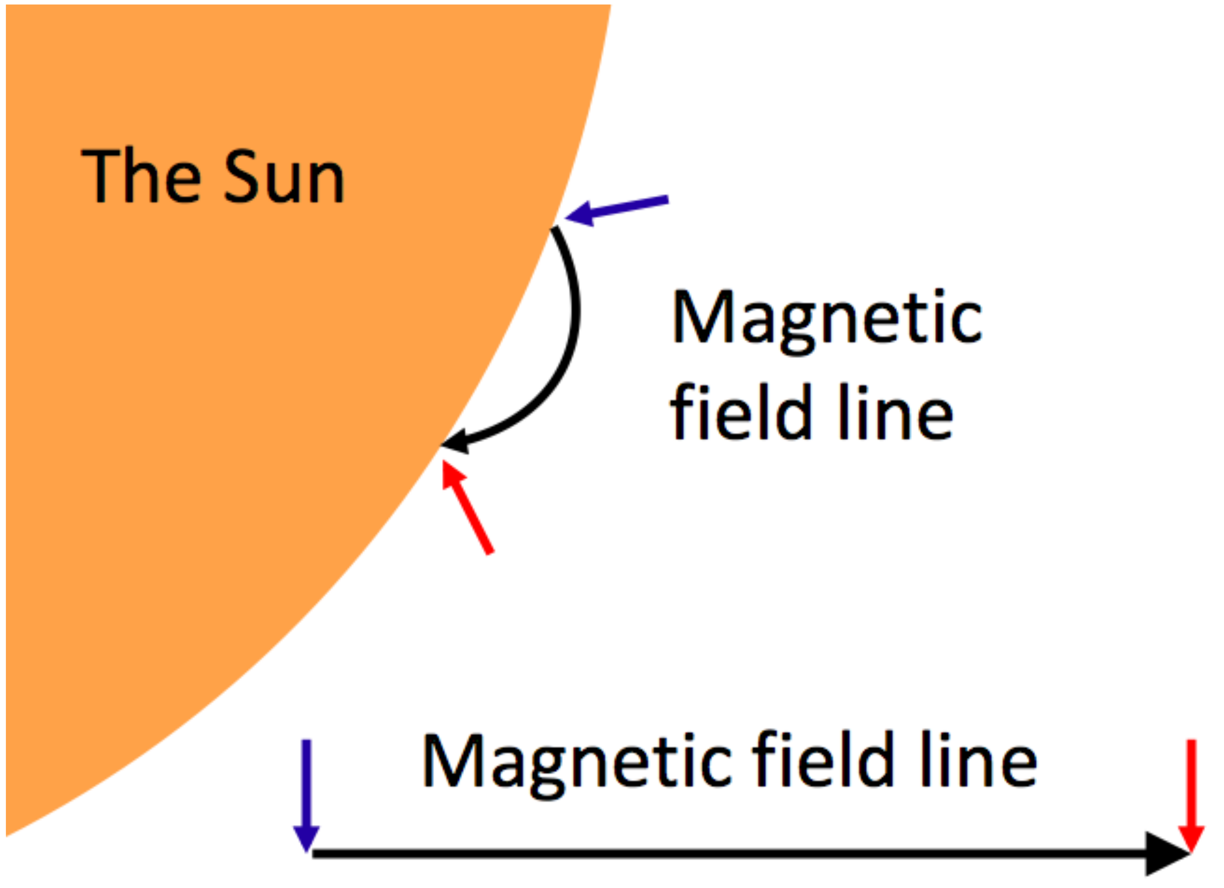
Figure 1.
A depiction of the simplification of the closed field lines of the magnetic field of the Sun. The curved magnetic field line is straightened so that geometrical factors can be ignored in the simulation. The colored arrows indicate the injection points of wave energy to the magnetic field line, blue being the parallel wave mode injection point and red being the anti-parallel wave mode injection point.

Figure 2.
Steady state of the simulation of a coronal loop with equal wave spectral energy density injections at both footpoints. Upper plots contain the parallel-propagating wave spectrum and bottom plots contain the anti-parallel-propagating wave spectrum. The plots on the left contain slices of the wave spectral energy density data at three locations, which are color coded to match the dashed lines on the contour plots. The normalization value for this simulation is , the loop size L = 10,000 km, and the spatial cell size km.

Figure 3.
The calculated bulk velocity of energetic particles normalized to the Alfvén velocity in simulations of a coronal loop with the size L = 10,000 km and the spatial cell size km. Different normalization values are denoted in the legend.
Figure 3.
The calculated bulk velocity of energetic particles normalized to the Alfvén velocity in simulations of a coronal loop with the size L = 10,000 km and the spatial cell size km. Different normalization values are denoted in the legend.

Figure 4.
The calculated mean free path of particles in simulations of a coronal loop with the size L = 10,000 km and the spatial cell size km. Different normalization values are denoted in the legend.
Figure 4.
The calculated mean free path of particles in simulations of a coronal loop with the size L = 10,000 km and the spatial cell size km. Different normalization values are denoted in the legend.

Figure 5.
The calculated diffusion lengths of energetic particles for simulations of a coronal loop with the size L = 10,000 km and the spatial cell size km. The curves are cut off to avoid presenting the diverging values of the diffusion length in the middle. Different normalization values are denoted in the legend.

Figure 6.
Steady state of the parallel-propagating wave mode of a simulation of a L = 30,000 km coronal loop with equal wave spectral energy density injections at both edges. The anti-parallel-propagating wave information is omitted due to symmetry with the parallel-propagating wave information. The plot on the left contains slices of the wave spectral energy density data at three locations, which are color coded to match to the dashed lines on the contour plots. The normalization value is .

Figure 7.
The calculated energetic particle bulk velocities for simulations of coronal loops with the sizes L = 10,000 km and L = 30,000 km. The 30,000 km loop, simulation has a spatial cell size km and the rest have a spatial cell size km. The loop lengths in kilometers and normalization values for the curves are displayed in the legend in the mentioned order.

Figure 8.
The calculated energetic particle mean free paths for simulations of coronal loops with the sizes L = 10,000 km and L = 30,000 km. The 30,000 km loop, simulation has a spatial cell size km and the rest have a spatial cell size km. The loop lengths in kilometers and normalization values for the curves are displayed in the legend in the mentioned order.
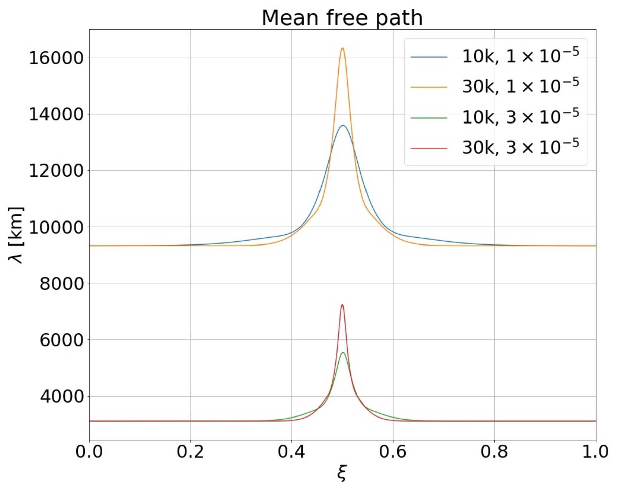

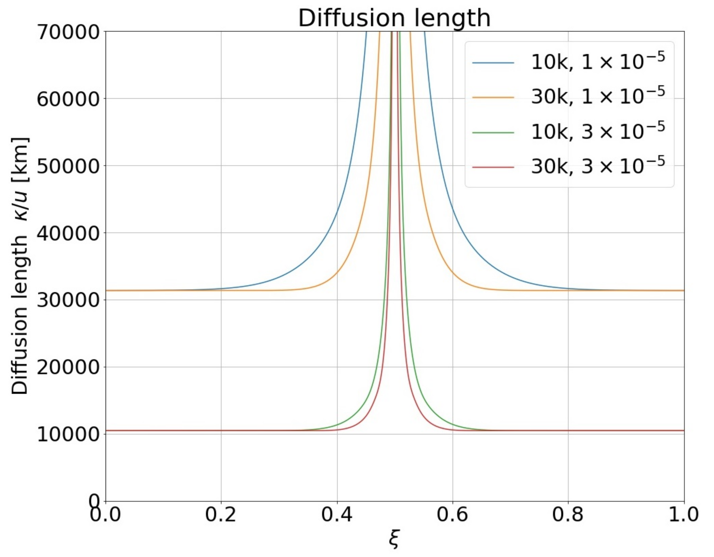
Figure 9.
The calculated energetic particle diffusion lengths for simulations of coronal loops with the sizes L = 10,000 km and L = 30,000 km. The 30,000 km loop simulation has a spatial cell size km and the rest have a spatial cell size km. The loop lengths in kilometers and normalization values for the curves are displayed in the legend in the mentioned order.

Figure 10.
The calculated stochastic acceleration rate of particles for simulations of coronal loops with the sizes L = 10,000 km and L = 30,000 km. The normalization value used for both simulations is . The longer loop has a spatial cell size km and the smaller loop km.
Figure 10.
The calculated stochastic acceleration rate of particles for simulations of coronal loops with the sizes L = 10,000 km and L = 30,000 km. The normalization value used for both simulations is . The longer loop has a spatial cell size km and the smaller loop km.

Publisher’s Note: MDPI stays neutral with regard to jurisdictional claims in published maps and institutional affiliations. |
© 2022 by the authors. Licensee MDPI, Basel, Switzerland. This article is an open access article distributed under the terms and conditions of the Creative Commons Attribution (CC BY) license (https://creativecommons.org/licenses/by/4.0/).
Share and Cite
MDPI and ACS Style
Nyberg, S.; Vainio, R. Simulating Three-Wave Interactions and the Resulting Particle Transport Coefficients in a Magnetic Loop. Physics 2022, 4, 394-408. https://0-doi-org.brum.beds.ac.uk/10.3390/physics4020026
AMA Style
Nyberg S, Vainio R. Simulating Three-Wave Interactions and the Resulting Particle Transport Coefficients in a Magnetic Loop. Physics. 2022; 4(2):394-408. https://0-doi-org.brum.beds.ac.uk/10.3390/physics4020026
Chicago/Turabian StyleNyberg, Seve, and Rami Vainio. 2022. "Simulating Three-Wave Interactions and the Resulting Particle Transport Coefficients in a Magnetic Loop" Physics 4, no. 2: 394-408. https://0-doi-org.brum.beds.ac.uk/10.3390/physics4020026