About the Data Analysis of Optical Emission Spectra of Reactive Ion Etching Processes—The Method of Spectral Redundancy Reduction

Abstract

In this study, we present the Method of Spectral Redundancy Reduction (MSRR) for analyzing OES (optical emission spectroscopy) data of dry etching processes based on the principles of spectral clustering. To achieve this, the OES data are transformed into abstract graph matrices whose associated eigenvectors directly indicate anomalies in the data set. We developed an approach that allows for the reduction in temporally resolved optical emission spectra from plasma structuring processes in such a way that individual emission lines can be algorithmically detected, which exhibit a temporal behavior different from the collective behavior of the temporally resolved overall spectrum. The proportion of emission lines that behave consistently throughout the entire process duration is not considered. Our work may find applications in which OES is used as a process-monitoring technique, especially for low-pressure plasma processing. The major benefit of the developed method is that the scale of the original data is kept, making physical interpretations possible despite data reductions.

1. Introduction

The complete analysis of large amounts of data from the optical emission spectra of dry etching processes requires mathematical methods from multivariate data analysis, such as PCA (Principal Component Analysis) or machine learning. Already 20 years ago, Shadmehr et al. [1] demonstrated that PCA can be used to predict process characteristics. Furthermore, machine learning is continuously gaining importance and gradually establishing itself as a control tool in the processing and analysis of optical emission spectra. Park et al. [2] employed machine learning to predict plasma parameters, specifically the electron density and electron temperature, from optical emission spectroscopy (OES) data. They propose the use of this method for the noninvasive determination of relevant plasma parameters. Clustering methods are also widely employed in the literature to evaluate OES data. For example, Jang et al. [3] applied a modified k-means algorithm to cluster emission lines and optimize endpoint detection for the patterning of silicon nitride. They introduce a time-resolved cluster validation factor to reliably separate the OES data set into two clusters—data before and after the endpoint. Lee et al. [4] published a similar approach to enhance the sensitivity of endpoint detection for silicon oxide patterning with a very low etch load, using a modified Gaussian mixture model for clustering instead of k-means. Additionally, Flynn and McLoone proposed the Max Separation Clustering method, which decomposes emission lines into different groups to analyze the temporal characteristics of emission data [5]. The methods based on clustering are mainly designed to detect the endpoint at the end of a dry etching process. However, a small amount of scientific reports currently describe methods for extracting the emission lines of a plasma process that have particular significance for that process. For example, Yang et al. [6] reported on a method that they named Internal Information Redundancy Reduction (IIRR). Their approach involves removing all wavelength variables that exhibit saturation at a given time point. This means that all lines showing temporal variation over the process time are detected. The advantage of this method lies in the fact that the data reduction occurs at the scale of the original data. This simplifies the interpretation of the obtained results, which can become complex when applying PCA to data from optical emission spectroscopy. This complexity arises from the fact that the calculated principal components are linear combinations of all discrete wavelengths [7], making it challenging to attribute observed effects solely to individual plasma species. Our method for reducing temporally resolved emission spectra allows us to still make statements about specific characteristics of the original data after dimension reduction. In this study, we demonstrate that the Method of Spectral Redundancy Reduction (MSRR) can be effectively used to identify spectral positions in the data set that deviate from the collective temporal behavior of the emission spectrum. The MSRR is also based on the concept of spectral clustering. However, in this study, we demonstrate that unconventional methods need to be employed for the spectral analysis of optical emission spectroscopy data, or existing approaches need to be expanded in order to make reliable assertions about a reduced data set. In particular, we show that anomalies can be read directly from the results by the skillful transformation of data matrices.

2. Theory

2.1. Spectral Clustering

An OES data set is typically organized in a matrix $\mathit{X}$, where the elements $x_{i,j}$ denote the intensities of emission lines at specific time points and corresponding wavelengths. Therefore, the rows of this matrix may represent the discrete time points, while the columns are associated with discrete wavelengths. The proposed approach of the MSRR is based on Spectral Clustering, as described in [8]. The objective of these methods is to identify groups within a data set so that variables within the same group exhibit high similarity while the variables from different groups exhibit low similarity to one another. These methods are based on graph theory. The collected measurement data $\mathit{X}$ are transformed into an abstract graph (or a graph matrix), which refers to the generation of a symmetric neighborhood matrix, also known as adjacency matrix $\mathit{A}$. The entries of $\mathit{A}$ contain information about the similarities or distances between the objects under investigation. In the context of graph theory, the objects being studied are referred to as the vertices of the graph, while the similarities or distances are understood as weighted edges [9]. Therefore, the adjacency matrix represents the connectivity pattern of the vertices in the graph. Consequently, each entry greater than 0 represents a connection (or edge) between two vertices of the graph. An important requirement for spectral clustering is that the calculated graph matrices do not contain loops, meaning that the main diagonal elements of the adjacency matrix must be zero. In a general form, the adjacency matrix associated with a matrix $\mathit{X}$ with q columns takes the following form:

$${\left(a_{ij}\right)}_{q,q}=\left\{\begin{array}{cc}{a}_{ij}\geqq 0\hfill & ,\mathrm{if}i\ne j\hfill \\ a_{ij}=0\hfill & ,\mathrm{if}i=j\hfill \end{array}\right.$$

(1)

In addition to the adjacency matrix, the degree matrix $\mathit{G}$ is defined as a diagonal matrix whose elements are the sums of the individual column vectors of $\mathit{A}$ [8]:

$$\mathit{G}=\mathrm{diag}\left(\sum _{i=1}^n{a}_{ij}\right)$$

(2)

Thus, the Laplacian matrix and normalized Laplacian matrices can be calculated as follows:

$$\mathit{L}=\mathit{G}-\mathit{A}$$

(3)

$${\mathit{L}}_{\mathrm{norm}}={\mathit{G}}^{-1}\mathit{L}$$

(4)

The fundamental principles of spectral clustering are described in [8]. In this study, Luxburg explains the basic functioning of the algorithm by using an example of randomized data, discussing both the Laplacian matrix and the normalized Laplacian matrix. Formally, the method consists of four main steps:

• Construction of the adjacency matrix.
• Computation of the (normalized) Laplacian matrix.
• Computation of the first k eigenvectors of the Laplacian matrix.
• Analysis of the eigenvectors.

2.2. Calculation of the Adjacency Matrix

Each spectral analysis requires an adjacency matrix $\mathit{A}$ from the given data $\mathit{X}$. However, $\mathit{A}$ is not uniquely defined in general because the similarity or distance values $a_{i,j}$ can be computed in different ways. Consequently, multiple adjacency matrices can be calculated for a given data set. In the following, the matrices will be named differently in order to distinguish them from each other. To construct an adjacency matrix, while considering that the data matrix $\mathit{X}$ is already presented in the form described above, the calculation rule of the Euclidean norm is used, which represents the distance of the column vectors ${\mathit{x}}_l$ and ${\mathit{x}}_m$:

$$d_{L2}({\mathit{x}}_l,{\mathit{x}}_m)=\sqrt{\sum _{i=1}^n{(x_{i,l}-x_{i,m})}^2}$$

(5)

Utilizing the binomial formula, Equation (5) can be reformulated:

$$\begin{array}{cc}\hfill d_{L2}({\mathit{x}}_l,{\mathit{x}}_m)& =\sqrt{\sum _{i=1}^n(x_{i,l}^2-2x_{i,l}{x}_{i,m}+x_{i,m}^2)}\hfill \end{array}$$

(6)

$$\begin{array}{cc}\hfill d_{L2}^2({\mathit{x}}_l,{\mathit{x}}_m)& =\sum _{i=1}^n{x}_{i,l}^2-2\sum _{i=1}^n{x}_{i,l}{x}_{i,m}+\sum _{i=1}^n{x}_{i,m}^2\hfill \end{array}$$

(7)

$$\begin{array}{cc}\hfill & =|{\mathit{x}}_l{|}^2-2\sum _{i=1}^n{x}_{i,l}{x}_{i,m}+{\left|{\mathit{x}}_m\right|}^2\hfill \end{array}$$

(8)

It can be observed that the first and last terms correspond to the squared magnitudes of the vectors associated with the variables or vertex for which the distance is to be determined. Additionally, the middle term represents the double scalar product of ${\mathit{x}}_l$ and ${\mathit{x}}_m$. According to the definition, scalar multiplication involves multiplying a row vector with a column vector. Hence, the vector ${\mathit{x}}_l$ needs to be transposed. This implies that

$$d_{L2}^2({\mathit{x}}_l,{\mathit{x}}_m)=|{\mathit{x}}_l^{\mathbf{T}}{|}^2-2·{\mathit{x}}_l^{\mathbf{T}}•{\mathit{x}}_m+{\left|{\mathit{x}}_m\right|}^2,$$

(9)

when examining the relationship between columns l and m of the given data matrix. To generalize this procedure to a data matrix $\mathit{X}$ with q columns, we start by multiplying the transposed data matrix with itself:

$${\mathit{X}}^{\mathbf{T}}\mathit{X}={\left(p_{ij}\right)}_{q,q}={\left({\mathit{x}}_i^{\mathbf{T}}•{\mathit{x}}_j\right)}_{q,q}$$

(10)

This operation calculates the scalar product for each pair of columns in the data matrix $\mathit{X}$, resulting in a $q\times q$ matrix. Taking the square root of the vector composed of the elements on the main diagonal of the matrix product yields the length of each column vector in $\mathit{X}$:

$$\mathit{b}=\sqrt{\mathrm{diag}\left({\mathit{X}}^{\mathbf{T}}\mathit{X}\right)}=\sqrt{{\left({\mathit{x}}_i^{\mathbf{T}}•{\mathit{x}}_i\right)}_{q,q}}=\left(\begin{array}{c}|{\mathit{x}}_1|\\ |{\mathit{x}}_2|\\ ⋮\\ |{\mathit{x}}_q|\end{array}\right)$$

(11)

With a matrix

$$\mathit{S}=\left(\begin{array}{cccc}{\mathit{b}}^2& {\mathit{b}}^2& \cdots & {\mathit{b}}^2\end{array}\right)=\left(\begin{array}{ccc}{s}_{11}& \cdots & s_{1q}\\ ⋮& \ddots & ⋮\\ s_{q1}& \cdots & s_{qq}\end{array}\right)\mathrm{with}{s}_{ij}={\left|{\mathit{x}}_i\right|}^2\mathrm{for}i\mathrm{and}j\mathrm{from}1\mathrm{to}q,$$

whose dimension is equal to ${\mathit{X}}^{\mathbf{T}}\mathit{X}$ and whose columns are all ${\mathit{b}}^2$, the adjacency matrix associated with the data matrix $\mathit{X}$, using the distance measure of the squared Euclidean norm, can be calculated by using

$${\mathit{A}}^2={\mathit{S}}^{\mathbf{T}}-2·{\mathit{X}}^{\mathbf{T}}\mathit{X}+\mathit{S}.$$

(12)

Taking the square root of each matrix element $a_{ij}^2$ then results in the Euclidean distance matrix, where the entries $a_{ij}$ correspond to the result of Equation (5):

$$\mathit{A}={\left(\sqrt{a_{ij}^2}\right)}_{q,q}={\left(d_{L2}({\mathit{x}}_i,{\mathit{x}}_j)\right)}_{q,q}$$

(13)

When the vector $\mathit{b}$, as defined in Equation (11), is multiplied by its transpose, a matrix with elements $b_{ij}$ is obtained, which contains the products of the magnitudes of all column vectors of $\mathit{X}$ with each other:

$${\left(b_{ij}\right)}_{q,q}=\left(\mathit{b}•{\mathit{b}}^{\mathbf{T}}\right)={\left(|{\mathit{x}}_i\left|\right|{\mathit{x}}_j|\right)}_{q,q}$$

(14)

By normalizing each entry $p_{ij}$ of ${\mathit{X}}^{\mathbf{T}}\mathit{X}$ with $b_{ij}$, it is possible to construct a similarity matrix whose entries correspond to the cosine of the angle between the column vectors of $\mathit{X}$:

$$\mathit{A}={\left(\frac{p_{ij}}{b_{ij}}\right)}_{q,q}={\left(\frac{{\mathit{x}}_i^{\mathbf{T}}•{\mathit{x}}_j}{|{\mathit{x}}_i\left|\right|{\mathit{x}}_j|}\right)}_{q,q}={\left(cos<)({\mathit{x}}_i,{\mathit{x}}_j)\right)}_{q,q}$$

(15)

The measure of similarity of $\mathit{A}$ is referred to as the cosine similarity. Furthermore, the similarity matrix (Equation (15)) can be transformed by using

$$cos{\left(x\right)}^2+sin{\left(x\right)}^2=1$$

(16)

into an adjacency matrix with values representing the unsimilarity of the columns with each other:

$$\mathit{A}={\left(\sqrt{1-{\left(\frac{p_{ij}}{b_{ij}}\right)}^2}\right)}_{q,q}={\left(sin<)({\mathit{x}}_i,{\mathit{x}}_j)\right)}_{q,q}$$

(17)

The entries $a_{ij}$ of this matrix $\mathit{A}$ contain information about the differences between the considered vertices, similar to the case when using the Euclidean norm (Equation (13)). It should be noted that in this adjacency matrix, the loops in the graph are eliminated solely through the calculation rule. In contrast, in Equation (15), this elimination must be performed separately (e.g., by subtracting $\mathit{A}$ from a diagonal matrix with the same main diagonal elements, $\mathit{A}-\mathrm{diag}\mathit{A}$).

2.3. Calculation of the Gaussian Similarity

Each given $\mathit{A}$ with its distance entries $a_{ij}$ can be transformed into an adjacency matrix by element-wise applications of the Gaussian similarity function. The individual edge weights $g_{i,j}$ are then determined by the Gaussian similarity. However, the resulting loops must be removed after the application. The entries of the Gaussian similarity matrix are then

$${\left(g_{ij}\right)}_{q,q}=\left\{\begin{array}{cc}{g}_{ij}=exp\left(\frac{-a_{ij}^2}{2{\sigma }_i{\sigma }_j}\right)\hfill & ,\mathrm{if}i\ne j\hfill \\ g_{ij}=0\hfill & ,\mathrm{if}i=j.\hfill \end{array}\right.$$

(18)

However, the calculation of $g_{ij}$ is not unique, as any type of distance or similarity measure can be used for $a_{ij}$. Additionally, the parameter ${\sigma }_i$ (or ${\sigma }_j$) is arbitrarily chosen (in [8], ${\sigma }_i={\sigma }_j=1$ is set) and, based on our literature research, does not have a well-defined determination procedure. According to Zelnik-Manor and Perona [10], $g_{i,j}$ can be “locally scaled” by the parameter $\sigma$. Each vertex ${\mathit{x}}_i$ of the graph has its “own” scaling parameter ${\sigma }_i$, which is determined by the distance $a_{ij}$ of a neighboring vertex ${\mathit{x}}_j$ (not necessarily the direct neighbor). Hence, in Equation (18), ${\sigma }_i{\sigma }_j$ is used instead of the usual ${\sigma }^2$ in the Gaussian equation. The approach of [10] was adopted and varied by Kong et al. The authors propose determining ${\sigma }_i$ not only based on a single nearby vertex but also by considering a certain number of surrounding vertices around ${\mathit{x}}_i$ [11]. They compute ${\sigma }_i$ by using the distances of the K nearest neighbors, applying the equation

$${\sigma }_i=\sum _{j=1}^K\frac{1}{{\sum }_{k=1}^L\frac{1}{a_{jk}}}=\sum _{j=1}^K\frac{1}{\frac{1}{a_{j,1}}+\frac{1}{a_{j,2}}+\frac{1}{a_{j,3}}+\cdots +\frac{1}{a_{j,L}}}$$

(19)

where, in the cited source, $L=K$ is used (the explanation of L is given later). In Equation (19), the $a_{jk}$ represents the K smallest distances between vertex ${\mathit{x}}_j$ and its nearest K neighbors (the index variables j and k do not correspond to matrix indices here). The scaling parameter for vertex ${\mathit{x}}_i$ is thus not determined by the distances or edge weights between ${\mathit{x}}_i$ and its immediate neighboring vertex, but rather by the edge weights between ${\mathit{x}}_j$ and their nearest neighbors, excluding ${\mathit{x}}_i$. In a more intuitive sense, Equation (19) can be interpreted as the “collective impact” of K neighbors on vertex ${\mathit{x}}_i$. The individual impact of a vertex ${\mathit{x}}_j$ is determined by the sum of the inverted distances to its own K nearest neighbors. This quantity is referred to as the edge impact. However, when determining the scaling factor ${\sigma }_i$ according to [11], the edge impact of ${\mathit{x}}_i$ itself is neglected. Although an approach to formulate it for ${\mathit{x}}_i$ was not found, the overall edge impact resulting from all vertices in the graph can still be determined. ${\sigma }_i$ for vertex ${\mathit{x}}_i$ can then be described not as the impact of its neighbors on it but indirectly as the effective impact in the graph region around ${\mathit{x}}_i$. One simple solution is to calculate the scaling factor ${\sigma }_i$ by summing up all the K overall edge impacts in the graph region around ${\mathit{x}}_i$. The calculation of ${\sigma }_i$ is modified in this study and is performed as follows:

$${\sigma }_i=\sum _{j=1}^K{\sigma }_j=\sum _{j=1}^K{\left(\sum _{k=1}^K\frac{1}{{\sum }_{l=1}^L\frac{1}{a_{kl}}}\right)}_j.$$

(20)

Each individual term ${\sigma }_j$ in Equation (20) is determined based on the procedure described in [11] (Equation (19)). Thus, they represent the respective collective impacts on the vertices from $j=1$ to K, where $j=1$ corresponds to the collective impact on vertex ${\mathit{x}}_i$. Note that by including the reference vertex ${\mathit{x}}_i$, K now refers to all the contributing vertices, and the number of influencing neighboring vertices becomes $(K-1)$. Another difference from Kong et al. [11] is the parameter L, which is chosen in the interval $\{3K\dots 4K\}$. This interval was found to be practical within the scope of this study. This means that the number of necessary neighboring vertices L and $(K-1)$ are separately chosen for the calculation of the edge impact and collective impact in order to compute the individual entries of the Gaussian similarity matrix.

3. Materials and Methods

3.1. Algorithms of the MSRR

For the OES data analysis, the principles described above were transferred to specific algorithms. Each tested similarity measure was calculated by using a programmed function, which returns the pairwise distances or similarities between the recorded wavelengths. The input data matrix for each function was prepared similarly, according to predefined criteria, by using an algorithm. The basis for determining an adjacency is always Equation (10) in combination with Equation (11). Therefore, it is sufficient to formally apply Equation (10) to the data matrix and store the main diagonal of the product as a column vector. Based on this, the desired adjacency matrix can then be further calculated.

3.1.1. Euclidean Distance

To calculate the Euclidean distance matrix (Equation (13)), it should be noted that the used algebra software (octave) works with row vectors by default, which is why the subalgorithm deviates from the formulation in Section 2. The squares of the absolute values of the main diagonal of the matrix product are introduced as a column vector by using Equation (11). However, in the program code, its square is stored as a row vector. The squares of the absolute values are not determined by ${\mathit{X}}^{\mathbf{T}}\mathit{X}$ but by squaring all the elements of the data matrix and then using the row sums as a row vector. Instead of using $\mathit{S}$, ${\mathit{S}}^{\mathbf{T}}$ is calculated to apply Equation (12). The details for calculating the Euclidean distance matrix can be found in Algorithm 1.

Algorithm 1: Calculation of the Euclidean distance

Input   : Data matrix $\mathit{X}$ with q columns and n rows     Output: Distance matrix $\mathit{A}$ of dimension $q\times q$ 1 Square the entries of $\mathit{X}$; 2 Calculate the q column sums of the squared entries; 3 Generate a row vector $\mathit{s}$, such that $\mathit{s}=\left({\sum }_{i=1}^m{x}_{i,1}^2,{\sum }_{i=1}^m{x}_{i,2}^2,{\sum }_{i=1}^m{x}_{i,3}^2,\dots ,{\sum }_{i=1}^m{x}_{i,\mathrm{q}}^2\right);$ 4 Repeat $\mathit{s}$ q times vertically to create the matrix ${\mathit{S}}^{\mathbf{T}}$; 5 Calculate the squared Euclidean distance matrix ${\mathit{A}}^2$ by applying Equation (12); 6 Take the square root of all entries of ${\mathit{A}}^2$ to compute the Euclidean distance matrix $\mathit{A}$ (see Equation (13))

3.1.2. Cosine and Sine Similarity

While an alternative calculation method is used for the Euclidean distance matrix, the Equations (10), (11), (14) and (15) can be implemented almost directly for the cosine similarity matrix. This is achieved by using the Octave function $\mathrm{diag}\left(\right)$, which returns the main diagonal of a matrix as a column vector. This means that the necessary normalization factors for each element of the matrix product are easily accessible and can be determined and used further through Equation (14). Algorithm 2 illustrates the steps for calculating the cosine similarity matrix.

Algorithm 2: Calculation of the cosine similarity matrix

Input   : Data matrix $\mathit{X}$ with q columns and n rows     Output: Similarity matrix $\mathit{A}$ of dimension $q\times q$ 1 Calculate the matrix product with the elements $p_{ij}$: $\mathit{P}={\mathit{X}}^{\mathbf{T}}\mathit{X}$ (see (10)); 2 Define a column vector with the absolute values of the column vectors of $\mathit{X}$: ${\mathit{b}}^{\mathbf{T}}=(\sqrt{p_{11}},\sqrt{p_{22}},\sqrt{p_{33}},\dots ,\sqrt{p_{q-1q-1}},\sqrt{p_{qq}})$ (see Equation (11)); 3 Calculate the pairwise products of the absolute values of all columns of $\mathit{X}$ using Equation (14): $\mathit{B}=\mathit{b}•{\mathit{b}}^{\mathbf{T}}$; 4 Calculate the cosine similarity matrix using Equation (15): $\mathit{A}={\left(\frac{p_{ij}}{b_{ij}}\right)}_{q,q}$ for $i=1$ to q and $j=1$ to q

By using Equation (16), the two trigonometric functions $sin\left(x\right)$ and $cos\left(x\right)$ are related. This means that Algorithm 2 can be directly used to calculate the sine similarity in the first step. Solving Equation (16) for $sin\left(x\right)$ then provides the squared sine values. Taking the square root of the elements of the resulting matrix results in the sine similarity (see Algorithm 3).

Algorithm 3: Calculation of the sine similarity

Input   : Data matrix $\mathit{X}$ with q columns and n rows     Output: Adjacency matrix $\mathit{A}$ of dimension $q\times q$ 1 Calculate the cosine similarity matrix using Algorithm 2; 2 Calculate ${\mathit{A}}^2$ using Equation (16), where the equation is solved for $sin{\left(x\right)}^2$; 3 Take the square root of all entries of ${\mathit{A}}^2$ to compute the adjacency matrix (see Equation (17))

3.1.3. Gaussian Similarity

The calculation of the Gaussian similarity matrix follows Equation (18) and is shown as Algorithm 4 below. For the input distance measure, one of the Algorithms 1–3 is used. To determine the scaling parameter (Equations (19) or (20)), the graph needs to be loop-free (i.e., the main diagonal elements must be set to zero when using Algorithm 2). Based on the resulting vertices degrees, the necessary number of neighbor vertices involved in calculating the scaling parameter is determined. To apply Equations (19) and (20), each row or column index of the adjacency matrix is considered as the number of a vertex (the matrix is symmetric, so the row index is sufficient). The columns of the adjacency matrix are sorted in increased order. At the same time, the row indices are stored in a separate index matrix according to the sorting order. In this specific case, the first row of the index matrix contains the numbers from 1 to q in increasing order because the main diagonal elements are zero—the distance from a vertex to itself is the smallest. Both matrices are reduced by deleting the first row and using only the top rows starting from the second row (for the adjacency matrix up to row L and for the index matrix up to row K). The entries of the reduced index matrix uniquely identify the nearest neighbors for each vertex in the graph. The column vectors of the sorted (reduced to L rows) adjacency matrix are then combined according to the index matrix. Specifically, the entries of the column vectors of the (reduced to K rows) index matrix determine the order in which the columns of the (reduced) adjacency matrix are chained. For example, if the first column vector of the (reduced) index matrix returns the values 4, 9, 2, and 7 for a choice of $K=5$ (considering 4 neighboring vertices), the fourth, ninth, second, and seventh columns of the (reduced) adjacency matrix are placed side by side in this order. This concatenation continues from the second column to the last column of the reduced index matrix. All entries are then inverted and summed column-wise. Each element of the resulting row vector corresponds to the denominator of Equation (19), the edge impact of each vertex. To determine the collective impact on each node, the reshaped row vector is considered. Refer to Figure 1 for an illustration (where the representation is limited to a graph with 5 vertices and considering 3 neighboring vertices; $K=4$).

Algorithm 4: Calculation of the Gaussian similarity

Input   : Data matrix $\mathit{X}$ with q columns and n rows     Output: Adjacency matrix $\mathit{A}$ of dimension $q\times q$ 1 Calculate the adjacency matrix using one of the Algorithms 1, 2, or 3; 2 If necessary: Remove loops of the graph; 3 Calculate the number of impacting neighboring vertices using: $$K=\frac{max\left\{M\right\}}{\overline{M}}\mathrm{where}M=\left\{\sum _{i=1}^q{a}_{i1};\sum _{i=1}^q{a}_{i2};\sum _{i=1}^q{a}_{i3};\dots ;\sum _{i=1}^q{a}_{ij};\dots ;\sum _{i=1}^q{a}_{iq}\right\}$$ if ($K<4$) $K=4$ (the smallest distance to a node is 0; with $K=4$, 3 neighboring nodes are considered) $L=3K\dots 4K$; 4 Sort each column of the adjacency matrix in increasing order and store each original row index in an index matrix ${\mathit{I}}_{idx}$; 5 Calculate a row vector with all edge impacts of each included neighboring vertex: Create an auxiliary matrix of dimension $L\times \left(\right(K-1)·q)$ where the entries follow the order of the reduced index matrix starting from the 2nd row; Invert all entries of the auxiliary matrix, except for the first row (the entries are 0); Calculate the column sums; 6 Calculate the collective impact on each individual vertex: Reshape the obtained row vector with $(K-1)·q$ columns into a matrix of dimension $(K-1)\times q$ Calculate the column sums of this matrix and store the result in a row vector; 7 Calculate the effective impact around each individual vertex in the graph: Generate an array where the row vector with the collective impacts is repeated vertically q times; Create a new row vector from the elements of the array, where the entries of the index matrix from row 1 to K determine which array entries are used and in which order they are set; Reshape the obtained row vector with $K·q$ columns into a matrix of dimension $K\times q$; Calculate the column sums of this matrix and store them in a row vector $\mathit{w}$; 8 Calculate the denominator of Equation (18) for each pairwise combination of the effective impacts (scaling parameters) using ${\mathit{w}}^{\mathbf{T}}•\mathit{w}$ and store a matrix with the elements $w_{ij}$; 9 Calculate for $i=1\cdots q$ and $j=1\cdots q$: $exp\left(\frac{-a_{ij}^2}{2w_{ij}}\right)$; 10 Replace the elements on the main diagonal with 0

   The row vector containing all the necessary edge impacts (the gray squares) is divided into equal segments, where the number of segments corresponds to the number of vertices in the graph, and each segment has the same number of elements (the number of neighboring vertices to be considered). The segments are transposed, and the segments are chained column-wise. Then, the column sums are calculated, which determines the collective impact (Equation (19)) of each vertex’s neighbors on the vertex. This vector is then repeated vertically as many times as the number of columns in the graph matrix dictates. The reduced index matrix determines the access to elements in the constructed array. The row access is given by the column number of the index matrix. The corresponding array columns are returned by the entries of the reduced index matrix. Applied to the example above, for the first column with entries 4, 9, 2, and 7, the access to elements in the array is (1,4), (1,9), (1,2), and (1,7), respectively. These are the collective impacts on the first 4 neighboring vertices of vertex 1, while the element (1,1) in the array represents the collective impact on the first vertex. The values are summed to obtain the effective impact in the graph area around vertex 1 (see Equation (20)). One “jumps” through the constructed array and records the obtained values in a row vector. For further calculation, Equation (18) requires the pairwise combination of all the scaling parameters. To calculate this, the constructed row vector is multiplied from the left with its transpose. Each entry of the input adjacency matrix is then normalized to the corresponding product of the scaling parameters, and the Gaussian similarity is determined. The equation inevitably leads to a similarity matrix with ones on the main diagonal. Finally, these elements are replaced by 0.

3.1.4. Full Algorithm of MSRR

The final procedure of the MSRR can be understood based on Algorithm 5. The input similarity matrix was defined as the sine similarity. The subsequent proposed calculation of the Gaussian similarity matrix is performed with $L=3K$, while the normalized Laplacian matrix is determined by using Equation (4). According to the principles of spectral clustering, the determination of the number of eigenvalues to consider is implemented in the MSRR too. Typically, the eigenvalues of the graph matrix are used for this purpose, and they are examined for a concept called the spectral gap [8]. However, based on our research, this approach is not applicable for analyzing OES data because the spectral gap cannot be reliably identified. Therefore, to determine the number of necessary eigenvectors, we implemented the algorithm proposed by [11] without any further restrictions. The authors determine the required number based on the analysis of cosine similarity between the rows of the eigenvectors. The goal is to find the cosine similarity matrix in which the entries strongly accumulate around the values of 0 and 1. This means that the number of values that significantly differ from 0 or 1 will be very small. In each iteration, starting from the second eigenvector, the cosine similarity matrix is computed multiple times by including the eigenvector corresponding to the next larger eigenvalue. The aim is to count (not sum) the values in the cosine correlation matrix that fall within the interval $[\xi ;1-\xi ]$. Here, $\xi$ is chosen to be close to zero. The necessary 2 to k eigenvectors are found when the count of the values falling within the interval $[\xi ;1-\xi ]$ is smaller for the first time compared to the counts obtained when the cosine similarity matrix is computed by using eigenvectors 2 to $k-1$ or 2 to $k+1$. In our final algorithm of the MSRR, the parameter $\xi$ is fixed at $0.001$ because we observed a negligible effect of this parameter in our study. The reduced spectrum is then obtained by calculating the variance over the number of columns used, from 2 to k, of the eigenvector matrix.

Algorithm 5: Method of spectral redundancy reduction

Input   : Data matrix $\mathit{X}$ with q columns and n rows     Output: Reduced spectrum (a vector of length q) 1 Calculate the adjacency matrix using Algorithm 4 Calculate the sinus similarity using Algorithm 3 Set the parameter L to $3K$; 2 Calculate the normalized Laplace matrix according to Equation (4); 3 Calculate the eigenvectors of the normalized Laplace matrix; 4 Determine the number k of eigenvectors to be included using the Algorithm from [11]; 5 Calculate the variance along the rows of the eigenvector matrix from column 2 to k

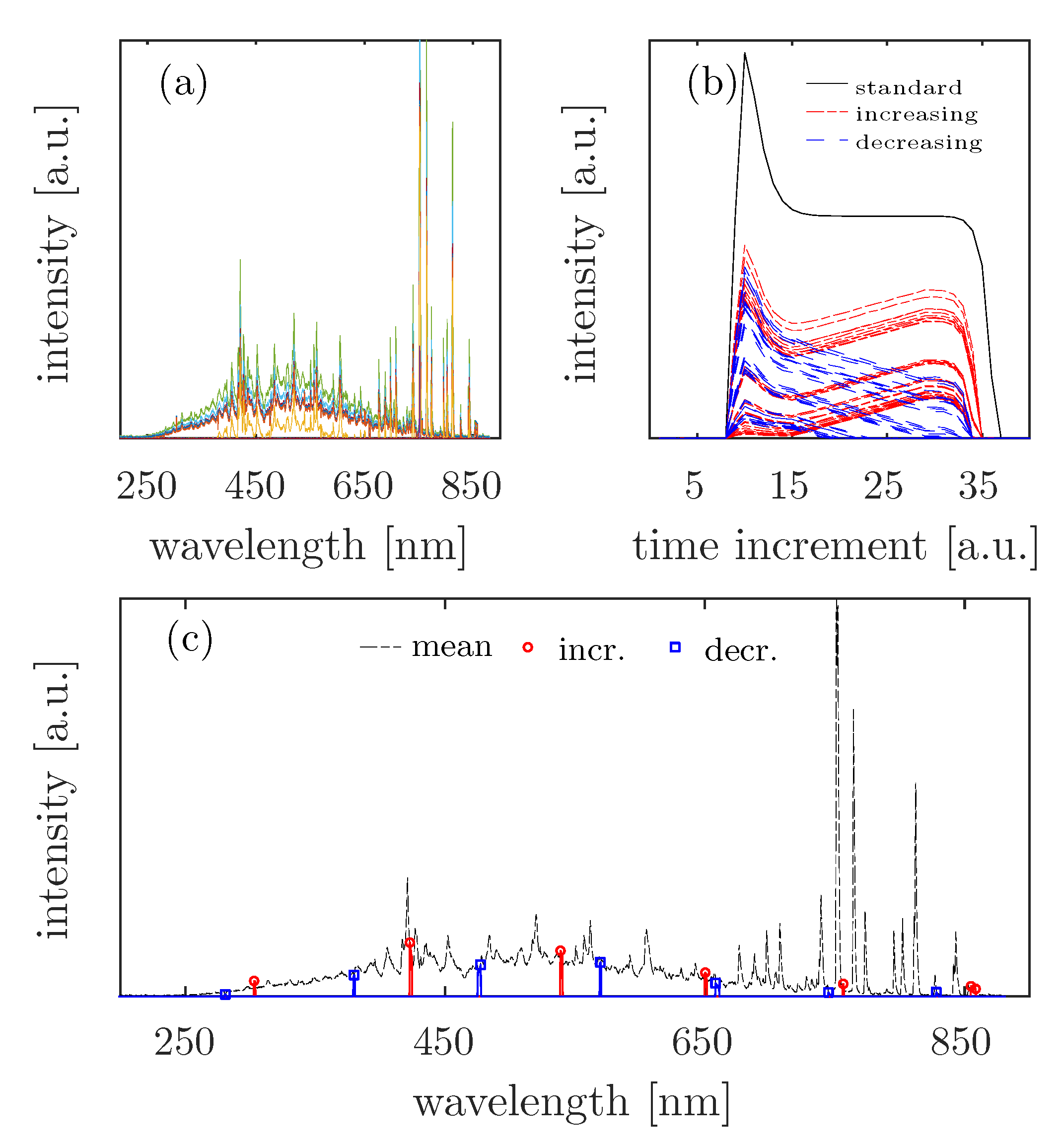
3.2. Generation of Test Data Sets

To assess the quality of a generated graph or evaluate the results obtained from a spectral analysis of the graph matrix, it is best to generate a test data set with known information before the analysis. The approach is based on investigating if implanted information in a test data set is actually detected after the data analysis. In this case, a single optical emission spectrum of an etching process is used to generate such a data set. To simulate the temporal intensity variation, the single measurement curve is repeated multiple times. In a matrix representation, the rows correspond to different time points and the columns correspond to wavelengths. The resulting matrix has a column count of q, representing discrete time points in each row. The artificially generated time-resolved emission spectrum should include plasma ignition and shut-off events. Both events are generated analytically across all columns (or wavelengths). Typically, optical emission measurements exhibit a curve with an initial intensity overshoot of individual emission lines. Without further physical significance, an initial time evolution is arbitrarily chosen based on Equation (21), with the shape-determining parameters arbitrarily selected. The first m rows of the test matrix, with row vectors of intensity ${\mathit{i}}_i$ (with $i=1$ to m), are created by

$${\mathit{i}}_i=\mathit{u}+\frac{3·\mathit{u}-\mathit{u}}{\tau }(i-k)exp\left(-\frac{i-k}{\tau }\right)\mathrm{für}i=\{1...m\}\mathrm{und}k>i,$$

(21)

where i represents the discrete time points, $\mathit{u}$ is the row vector with entries of the individual emission spectrum, $\tau$ is an arbitrarily chosen decay time, and k corresponds to the row index or time point at which the plasma ignition is simulated. All the rows generated by using Equation (21) with an index smaller than k result in entries smaller than zero, which are replaced with a zero entry. Similarly, the shut-off of the plasma is modeled in the same way, with an exponential decay in the intensity, now denoted as ${\mathit{o}}_i$ (with $i>m$):

$${\mathit{o}}_i={\mathit{i}}_i+(i-m)·(-1)exp(i-m).$$

(22)

The set of generated row vectors then yields a matrix of the following form:

$$\mathit{I}=\left(\begin{array}{ccccc}0& 0& 0& \cdots & 0\\ 0& 0& 0& \cdots & 0\\ 0& 0& 0& \cdots & 0\\ ⋮& ⋮& ⋮& & ⋮\\ I_{k,1}& I_{k,2}& I_{k,3}& \cdots & I_{k,q}\\ ⋮& ⋮& ⋮& & ⋮\\ I_{m,1}& I_{m,1}& I_{m,1}& \cdots & I_{m,q}\\ O_{1,1}& O_{1,2}& O_{1,2}& \cdots & O_{1,q}\\ O_{2,1}& O_{2,2}& O_{2,3}& \cdots & O_{2,q}\\ O_{3,1}& O_{3,2}& O_{3,3}& \cdots & O_{3,q}\\ ⋮& ⋮& ⋮& & ⋮\\ 0& 0& 0& \cdots & 0\\ 0& 0& 0& \cdots & 0\end{array}\right).$$

Until row k, their entries are all zero. At $i=k$, the plasma ignites. All the subsequent rows represent the evolution according to Equation (21) until time point m. The remaining entries $O_{i,j}$ follow the defined exponential decay after plasma shutdown (Equation (22)). In this form, the matrix does not contain meaningful information yet, as all the column vectors are nearly parallel and thus strongly linear dependent. Before composing the test spectrum, individual columns of the upper part of the matrix ($I_{i,j}$) are modified such that their entries are negatively correlated with each other, simulating the decrease or increase in the intensity of individual emission lines over time. The number and index of columns whose entries should decrease or increase across rows are randomized. To account for different peak widths, the randomly determined individual columns are combined with a random number of adjacent columns, symmetrically arranged around the initially determined columns. Only the degree of “temporal” change is determined by the prescribed increase. This results in individual wavelengths whose intensity increases with time while others decrease. The number of increasing lines is not necessarily equal to the number of decreasing lines. The indices of these columns (corresponding to wavelengths) are stored to compare them with the result of the analysis method later. Figure 2 illustrates such a data set.

The figure shows three individual plots. Panel (a) illustrates the change in all the column entries with an increasing row index—a generated temporal evolution of an emission spectrum. In panel (b), selected column entries are plotted against the row index, representing a time-dependent intensity measurement of selected wavelengths. The solid line (black) represents the standard case. The dashed lines represent all the columns in the data set that increase (red) or decrease (blue) with an increasing row index. The third plot (panel (c)) shows the average curve of the spectrum and the wavelength positions of the decreasing (☐) and increasing values (⃝   ). For the analysis of such artificial data, the threshold value $\xi$ required for the calculation of the reduced spectra was always chosen to be very small at ${10}^{-4}$ since the data are highly idealized and the implemented noise information is very small compared to the introduced variations.

3.3. Dry Etching Processes

To evaluate the MSRR on real data, the optical emission spectra of plasma-etching processes were recorded by using the USB2000 spectrometer (Ocean Optics, Orlando, FL, USA) with a sample rate of 10 Hz. The etching or structuring was performed on a DPS (decoupled plasma source) chamber of a Centura 5200 cluster system (Applied Materials, Santa Clara, CA, USA). The configuration of the plasma-etching chamber is based on the concept of inductive coupled plasma (ICP). We chose to investigate “easy” material-plasma systems, meaning that emission spectra from plasma-etching processes were used, where

• Layer materials consisting of a single component were etched.
• The layer to be etched did not have density gradients.
• Ideally, the material was completely removed, i.e., no mask materials generated additional plasma species contributing to the spectrum.
• The precursor mixture included only components that allowed for the clear identification of depletion effects (the intensity loss or increase caused by variations in species consumption or generation).

In particular, metal layers and semiconductor layers were sufficiently isotropic for the purpose used here. Additionally, these materials are partially plasma chemically etched by using a single gas. So, Germanium was structured in an SF₆-based plasma with a gas flow rate of 30 sccm; a process pressure of 10 mTorr; and coupled powers of 100 W and 500 W by using RF and ICP sources, respectively. Platinum structuring was performed with the process parameters of 100 sccm Cl₂, 50 sccm, 10 mTorr, 250 W bias power, and 100 W ICP power. Additionally, spectra from copper-etching processes based on hydrogen plasmas and titanium nitride-etching processes using pure Cl₂ plasmas were employed to test the MSRR.

4. Results

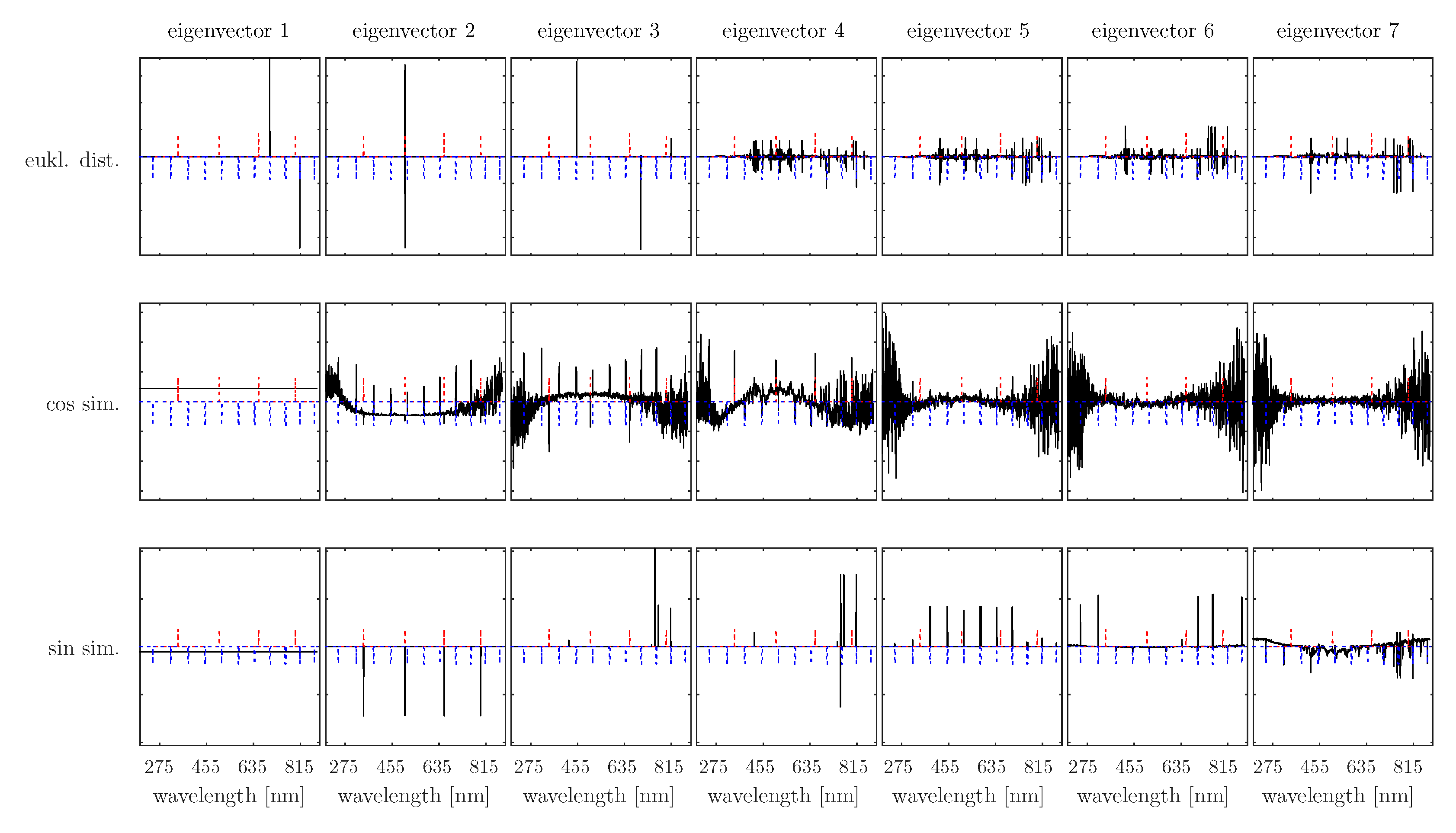
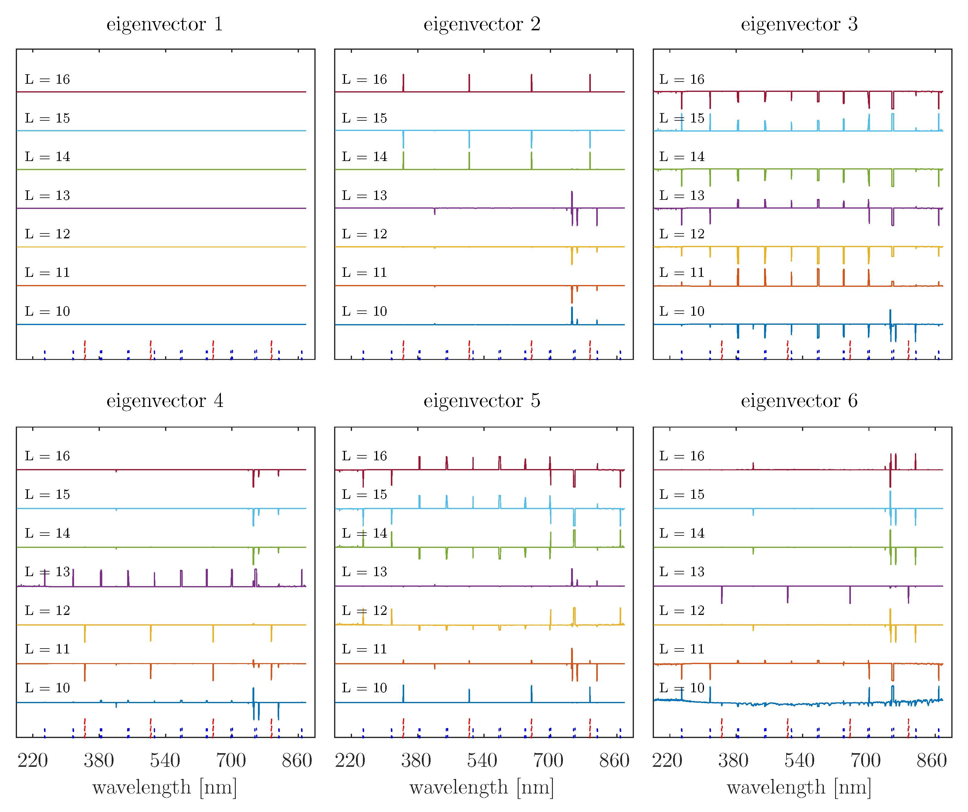
4.1. Eigenvector Analyses

For illustrative purposes, the results of the spectral analysis in this subsection are always discussed by using the same test data set to ensure comparability for result presentation. In Figure 3, the average spectrum and the corresponding randomly placed decreasing and increasing lines of the used test data set are shown. The positions of the varying columns (wavelengths) in the data set differ, due to randomized placement, from those shown in Figure 2. The wavelength positions of decreasing and increasing values are also symbolized here with ☐ in blue (flnd) and ⃝    in red (stgd).

Before starting to analyze the test data, it should be noted that the aim is not to find all the implanted information. The main focus is to identify changes in the data set.

Examples of the eigenvectors of graph matrices based on the different adjacency matrices are shown in Figure 4. Plotted are the first seven eigenvectors of the normalized Laplacian matrices (computed according to Equation (4)). For the calculation of the Gaussian similarity matrices, the approach of determining the local scale parameter (according to (19)) proposed by Kong et al [11] was used.

For all three distance measures, the local scaling parameters were calculated considering seven neighboring vertices ($K=8$, see Algorithm 4). The most notable are eigenvectors 2 to 6 in the last row of the figure, which are based on sine similarity. It can be observed that the peaks of these eigenvectors clearly indicate the artificially introduced variations in the data set. When cosine similarity is used (second row in the figure), there are also overlaps between the peaks of the eigenvectors and the implanted information, but there is significant noise in the outer regions of all the eigenvectors. In these regions, peaks of the eigenvectors are also located at positions of increasing or decreasing columns. In real-world scenarios, the spectral position of the variations in the data set is generally unknown (except for information about the endpoint), and any peaks in these outer regions might not be assigned any further significance. With the Euclidean distance measure, the first three eigenvectors do suggest some indication, but there is only a sparse agreement with the actual variations in the data set. Both the Euclidean norm and cosine similarity lose their relevance as input measures for an adjacency matrix for the analysis conducted here and are excluded from further analysis. Both the Euclidean norm and the cosine similarity lost their relevance as input measures for an adjacency matrix of the OES data and were therefore excluded by us in the development of the MSRR. At this point, it is important to inform the reader that within the scope of our study, we also examined nonmodified adjacency matrices and Gaussian similarity matrices with a constant scaling parameter. However, in all cases, we did not find any usable eigenvectors. According to [11], the choice of the number of neighboring vertices to be included appears to be arbitrary. If one iterates over the number of neighboring vertices for the calculation, different collective impacts (Equation (19)) are obtained for each iteration, resulting in different eigenvectors of the Laplacian matrix derived from the Gaussian similarity matrix. Refer to Figure 5, where K was increased from 4 to 10, resulting in seven different calculations.

In the diagrams, the first six eigenvectors are plotted against the wavelength axis for each iteration. The absolute values of the entries of the eigenvectors are generally of minor importance. To facilitate comparison, all the eigenvectors were normalized to their respective maxima and offsets along the ordinate axis based on the input value of K. In each diagram, the lowest eigenvector corresponds to the calculation with $K=4$, and the highest eigenvector corresponds to the calculation with $K=10$, indicating the inclusion of 3 to 9 neighboring vertices. All the eigenvectors in between are arranged in ascending order. Additionally, the implanted information is plotted in each diagram. To distinguish between increasing and decreasing columns, longer and shorter peaks are plotted below all the eigenvectors. As expected, the peaks of the eigenvectors tend to indicate the positions of increasing or decreasing columns in the data set. However, no discernible pattern is observed that would allow for further conclusions to be drawn. Particularly noteworthy are the two lowest first eigenvectors when using $K=4$ and 5. According to the principles of graph theory, the first eigenvector of a graph matrix should be the zero vector and contain only equal values (because in any case, the first eigenvalue of the graph matrix must be zero). Here, only the first eigenvalue should be zero, as the calculation generates a connected graph [8,9]. Obviously, when using 3 or 4 neighboring vertices, Gaussian similarity matrices are generated that are unsuitable for analysis. As K is increased, the properties of a connected graph are regained, and overlaps between the peaks of the eigenvectors are observed. However, it should be noted that the results depend on the manually set parameter K. When setting $K=6$ or 7, the second and fifth eigenvectors indicate the information. Still, the third and fourth eigenvectors do not provide significant information. Increasing the number further, the information provided by the second eigenvector remains the same, but now the fourth eigenvector indicates agreement with the positions of the decreasing columns in the data set. Due to the induced changes in the eigenvectors, the authors consider the method to be very sensitive to the parameter K. Regardless of the normalization of the Laplacian matrix, there is a risk of losing the desired information. In summary, there is a risk of obtaining false emission lines in the case of real data if the number of neighboring vertices is chosen unfavorably. In other words, when analyzing real recorded OES spectra, emission lines could be identified as deviating, but not differing from the collective behavior at all. The same applies to the reverse case, where emission lines with a significant difference in temporal behavior may not be detected. However, given that the eigenvectors indicate changes in the data set very well when K is chosen appropriately, the authors do not question the fundamental nature of the approach. Instead, the calculation of the collective impact based on Equation (19) is seen as unsuitable for evaluating data from OES. The result highlights the need for the modification of Kong et al.’s approach, as introduced in Section 2.3.

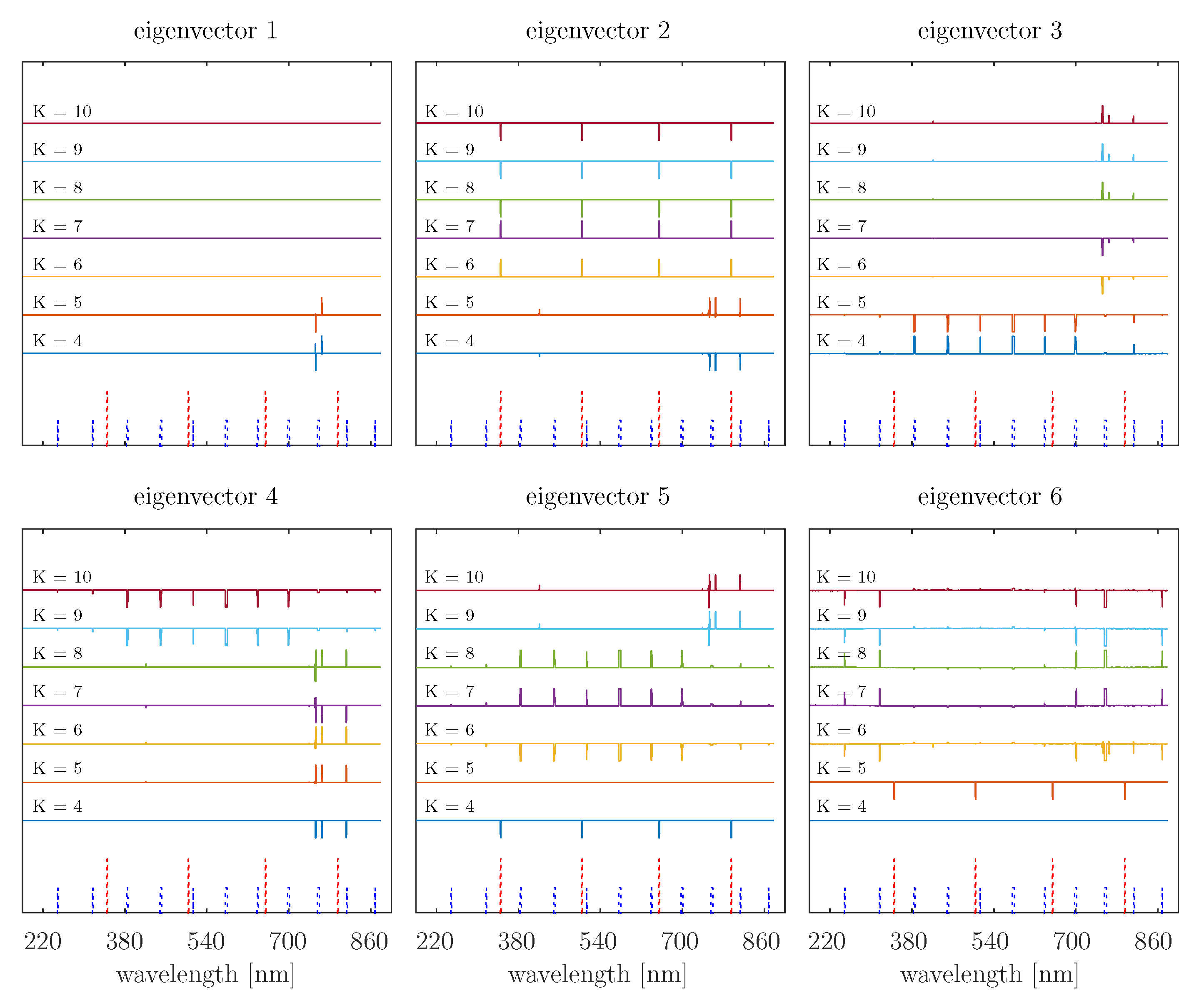
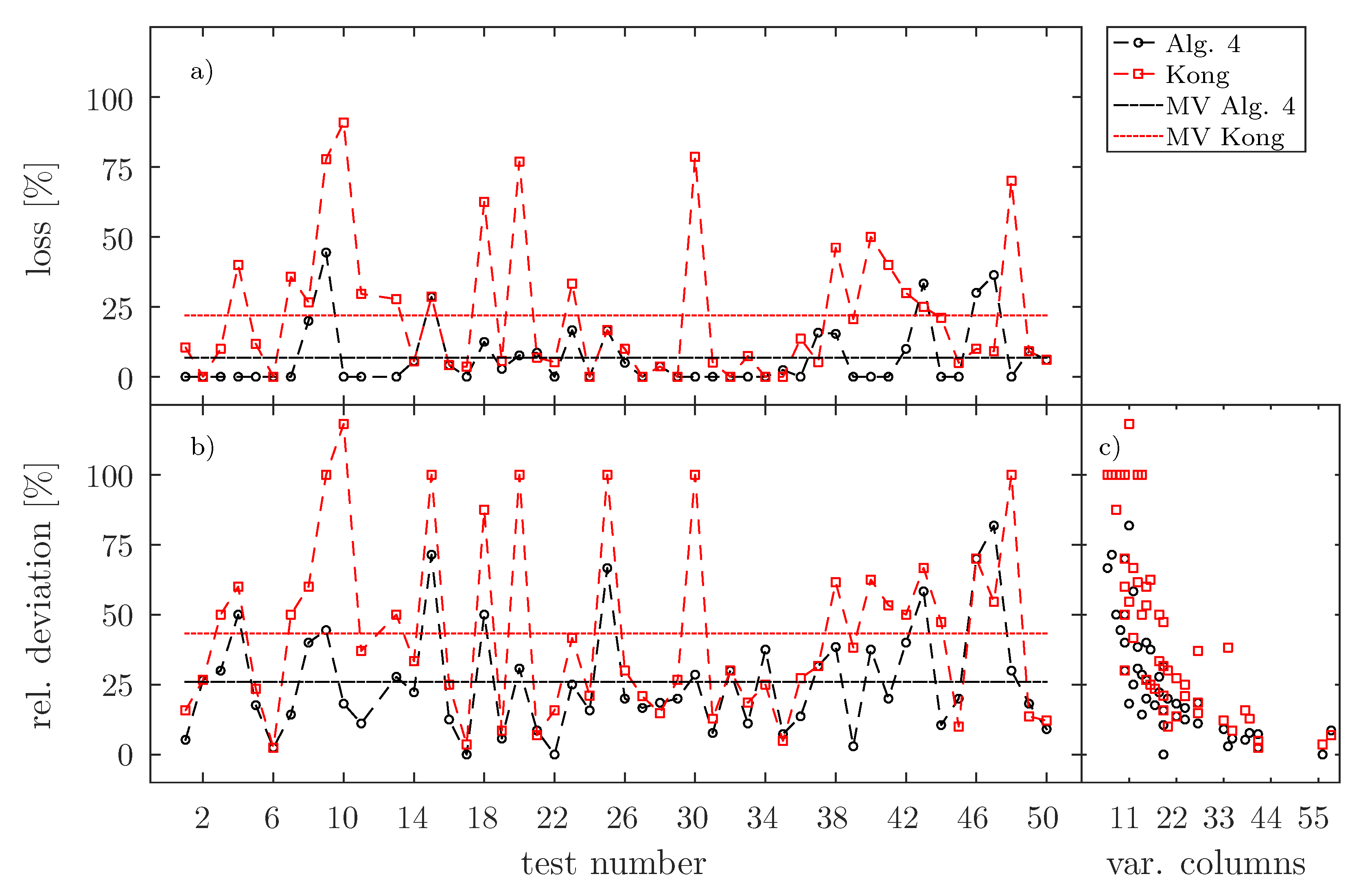
4.2. Application of the Proposed Calculation of the Gaussian Similarity Matrix

If the test is conducted as described above, using Algorithm 4, the result shown in Figure 6 is obtained. Rather than determining the collective impact and edge impact by using an equal number of neighboring vertices (Equation (19), with $K=L$), the scaling parameters ${\sigma }_i$ were calculated by iterating over the parameter L according to Equation (20), allowing for a variation in the number of vertices for the edge impact. In other words, instead of using K, iterations were performed over L ranging from 10 to 16.

In contrast to the application of Kong et al.’s method, for each iteration, the first eigenvector is always computed as the null vector. Furthermore, it must be reported that the calculation of K for this data set resulted in a value of three. According to the literature [10,11], the number of neighboring vertices to be included should be at least three. Therefore, the minimum value of K is four. Taking into account the explanations regarding Figure 5, it becomes evident that only the autarkic determination of K is insufficient to compensate for the inconsistencies found in the resulting eigenvectors. This indirectly justifies the need for a different approach to calculating the Gaussian similarity matrix for the analyses of OES data. However, it cannot be ruled out that there might be another way to calculate K such that Kong’s method can still be applied. In fact, the necessity to modify Kong’s method to compute the Gaussian similarity matrix results from the fact of using the K calculation.

With further comparisons of Figure 5 and Figure 6, it is evident that changes in the boundary region of the data set, particularly for wavelengths below 360 nm and above 720 nm, are more clearly indicated in the second case. While according to Kong et al.’s method, for K ranging from 6 to 10, based on a visual evaluation, all five eigenvectors (2–6) are needed, and the application of Algorithm 4 with $L=14$ to 16 fully suffices with only eigenvectors 2 and 3 to detect all the changes in the data set. Even for the incoming $L=11$ to 13, eigenvectors 2 to 4 would be sufficient (although the discussed boundary regions would be less discernible for $L=11$). Only for $L=10$ would all the displayed eigenvectors be required. Smaller values of L in these investigations lead to eigenvectors with peaks that less convincingly represent changes in the data set. This is also the reason for the investigation interval of $L=10\cdots 16$. Algorithm 4 appears to be less sensitive to the incoming parameter L in the range of 12 to 16 than the calculation method by Kong et al. about its input parameter K.

When considering the eigenvectors in Figure 6 from the perspective of spectral clustering, particularly focusing on eigenvectors 2 and 3 with an incoming $L=14$ to 16, the possibility of separating decreasing and increasing columns in the data set becomes evident. The peaks of eigenvector 2 consistently point in the opposite direction to the peaks of eigenvector 3. Compared to the embedded information, it can be seen that the second eigenvector exclusively indicates increasing columns, while the third eigenvector exclusively indicates decreasing columns in the data set. This demonstrates the potential, in terms of the optical emission spectroscopy of a plasma process, to distinguish between species consumption and species generation. However, this has not yet been achieved for two reasons: Firstly, consider the second eigenvector for the incoming $L=14$ and $L=15$. The peaks point in opposite directions. The assignment to columns with increasing values is only possible because the information is already known before the analysis. This is not always the case for real data. Assignment without further analysis of the nontransformed data is not possible. Secondly, despite the eigenvectors suggesting the possibility of grouping the peaks, this has not been achieved in this study thus far. The application of the k-means algorithm, commonly used for clustering [8], to the eigenvectors of the graph matrix did not yield reliable results in this study. Of course, it would be possible to “manipulate” the eigenvectors in the same way as in the representation of Figure 5 and Figure 6. However, such approaches were not further pursued, and the possibility of grouping emission lines remains for future studies.

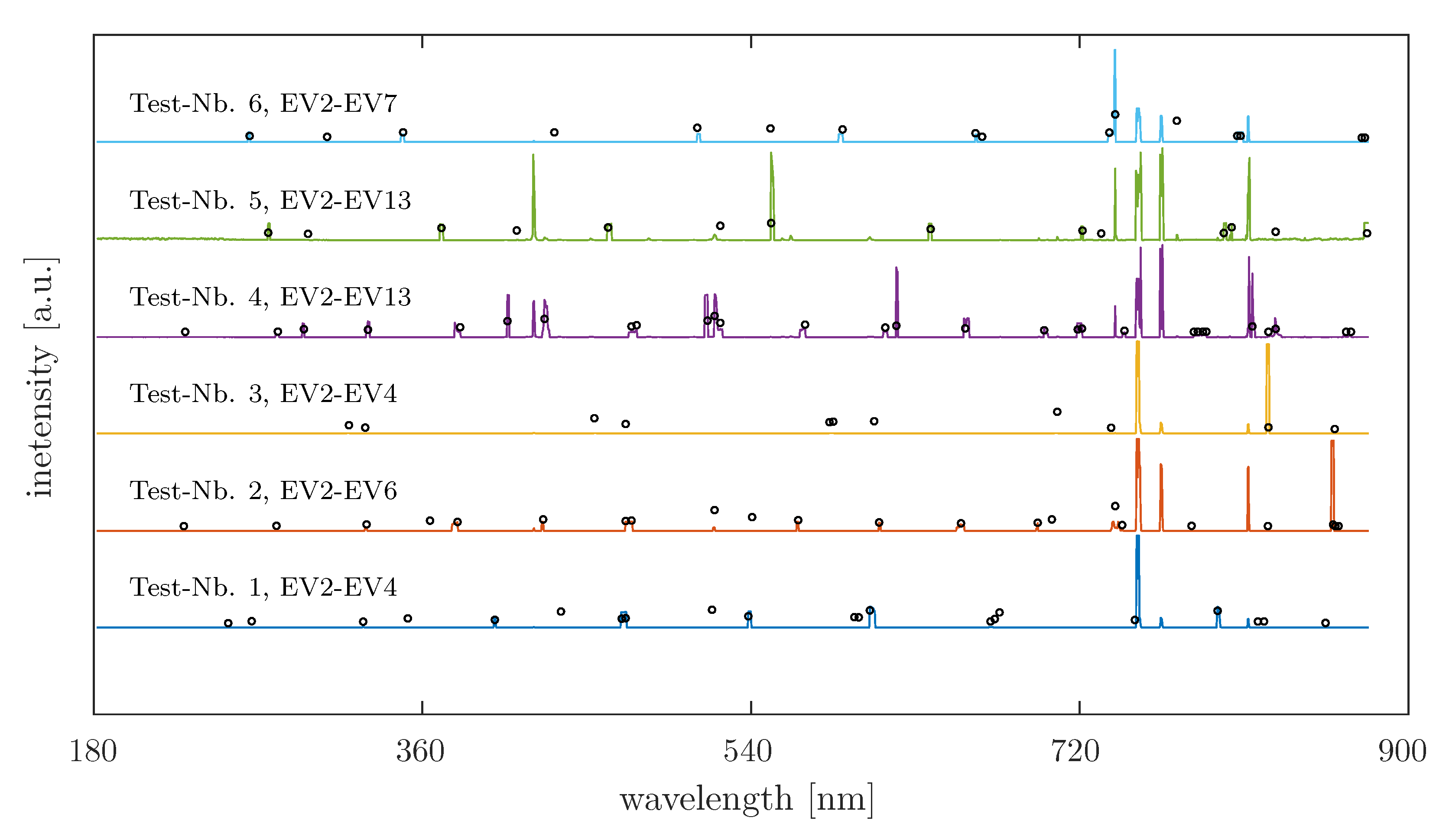
4.3. The Reduced Spectrum of Artificial Generated Data

The reduced spectrum refers to the variance over a previously determined number of eigenvectors of a graph matrix. When examining the effect of input parameters K and L, it was found that if the Gaussian similarity matrix is calculated by using the proposed method, the reduced spectrum appears to be less dependent on the input parameter L compared to the method by Kong et al. with the input parameter K. Therefore, L can be fixed at $L=3K$ for the proposed method of calculating the Gaussian similarity. Regarding the determination of the input parameter K, it was found during testing based on the same artificial input data that K should be fixed at six when using Kong’s method. Figure 7 and Figure 8 show two diagrams with six reduced spectra each, calculated based on artificial data.

The input adjacency is the sinus similarity in both cases. The difference lies in the calculation of the Gaussian similarity matrix. For Figure 7, Kong’s method was used, with the parameter K always chosen as six. The alternative approach introduced in this study is the basis for the reduced spectra in Figure 8. The necessary parameter L was redetermined for each calculation as $L=3K$. The data basis was the same for each calculation. This means that when a data set with randomly set information was generated, the reduced spectrum was calculated by using both variant 1 (Gaussian similarity according to Kong et al.) and variant 2 (an introduced alternative approach). For each individual spectrum, the randomly set changing wavelength positions are marked with ⃝   , indicated at the same positions in both figures. It is immediately apparent that not every implemented change is returned. The results also appear comparable. However, if the set variation that is not detected in the reduced spectrum is counted, it will be found that for this snapshot, $38\%$ of the variations in the data set are not detected when the Gaussian similarity is calculated by using Kong’s method. In contrast, there is an information loss of $12\%$ when our approach is used to calculate the reduced spectrum. Furthermore, it can be seen that in both cases, a change is always indicated at 752 nm, even though a change is not always set at that position. This is particularly noticeable in the third test in the diagrams, where the number of set variations is relatively small. The position corresponds to the highest peak in the mean spectrum (see Figure 3). When generating the test data, all the columns of the input matrix are subject to Equations (21) and (22). As a result, columns with very small entries reach the value zero faster than entries with large numerical values. Therefore, there is a weaker correlation between such columns compared to those with equivalent entries. For this reason, the eigenvectors indicate the pronounced peak especially when there is seldom actually set information. Consequently, the existence of the peak in the reduced spectrum should not be considered an error. However, both the information loss and additional found peaks must be considered when making a statement regarding the better suitability of either method. The result for 50 data sets with differently set information is summarized in Figure 9.

The diagram is divided into three parts. Figure 9a) shows the information loss, i.e., the part of the set-varying columns that were not found again in the reduced spectrum for both variants. Figure 9b) shows the relative deviation of the reduced spectrum compared to the implemented variation in the data set. The absolute deviation is obtained from the sum of the nonfound and nonset but detected variations. Figure 9c) shows the relationship between relative deviation and the number of varying columns in the data set. In the entire diagram, the relative values for variant 1 (Kong et al.) are denoted with ☐, and for variant 2 (Algorithm 4) with ⃝   , while the lines represent the means. It can be seen that the information loss is lower when the Gaussian similarity is calculated by using Algorithm 4. In this series of experiments, 95 % of the set information was found when using the proposed calculation method, whereas for the approach by Kong et al., 84 % can be indicated. On average, with variant 2, 7 % of the information contained in the data set is not found, while with variant 1, 22 % can be reported. Looking at the relative deviations (Figure 9b), the situation is similar. Here, it can be seen that the deviations from the implemented information for the reduced spectrum are lower on average for variant 2 than for variant 1. For both variants, very large deviations are observed in some cases. These occur when the implemented number of varying columns is small, which can be observed with the plot in Figure 9c). Over these 50 experiments, variant 1 has an average deviation of 43 %, while variant 2 can be indicated as 26 %. Obviously, the reduced spectrum is more dominated by differences in the values in the underlying data matrix when using variant 1, especially when there are few variations. The proposed modification of the approach by Kong et al., i.e., calculating the Gaussian similarity matrix by using the introduced effective impact (Equation (20)), seems to create a benefit. Due to the summarized results in Figure 9, we decided to implement Algorithm 4 in the Method of Spectral Redundancy Reduction (Algorithm 5), and the calculation method according to Kong et al. was not used.

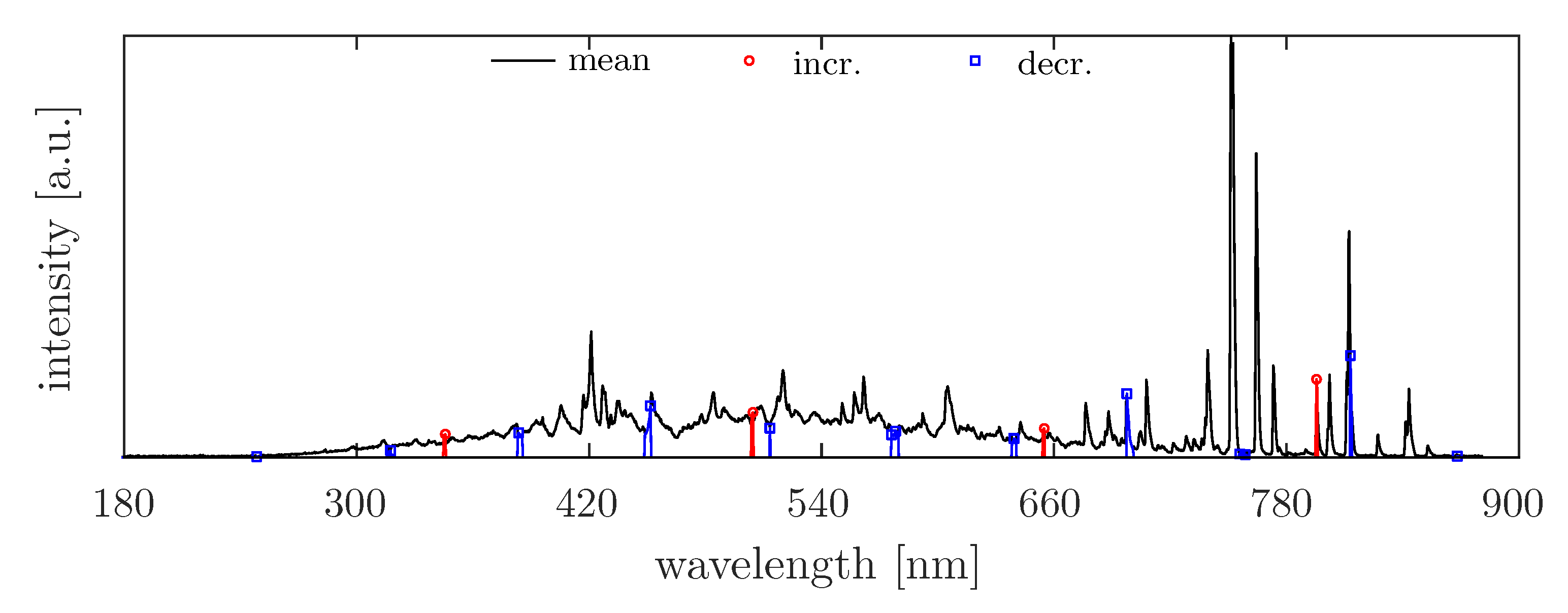
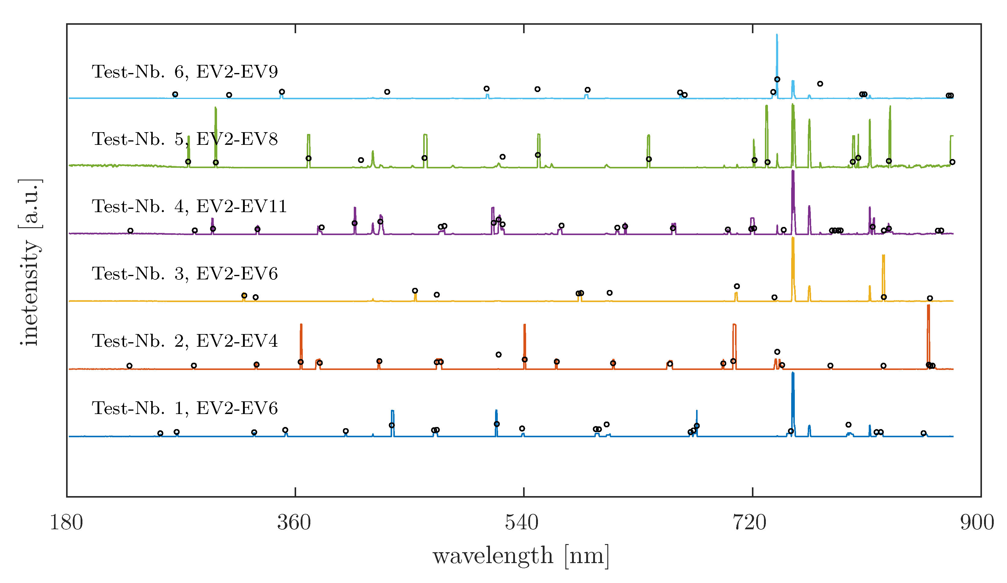
4.4. Analysis of Real OES Data

To demonstrate the effect of the parameter $\xi$ on the reduced spectrum, the result of the MSRR for a chlorine-based TiN etching is shown in Figure 10.

Two diagrams are presented, analyzing the optical emission of a 25-second titanium nitride-etching process. In this process, titanium nitride was not structured but etched uniformly without complete removal. The left diagram shows the mean spectrum and four reduced spectra, calculated with increasing values of $\xi$ from ${10}^{-4}$ to $5·{10}^{-3}$. The right diagram depicts the time dependence of different emission lines of the real data. The used eigenvectors for each reduced spectrum are indicated in the figure too. In this case, the parameter $\xi$ does not influence the reduced spectrum, as eigenvectors 2–6 consistently capture the variation in the data set for each $\xi$. A total of seven peaks are detected, with each peak marked by a different symbol in the mean spectrum. The same symbols can be found in the right diagram, allowing the individual time evolutions to be assigned to the peaks indicated in the reduced spectrum. The dashed lines represent selected emission lines not marked in the mean spectrum, included for comparison purposes. All the emission lines found in the reduced spectrum exhibit differences in their temporal behavior, showing an increase in the signal compared to the other comparison temporal behaviors provided. The legend additionally indicates the plasma species to which the identified emission lines are attributed (the information was obtained from the NIST Atomic Spectra Database [12]). These plasma species are atomic chlorine and titanium, with the most significant change observed for Cl.

Regarding the extraction of variable emission lines, a similar result was obtained when analyzing the optical emission spectra of a 150-second copper-etching process. In this process, copper was also not structured but completely removed. The result is shown in Figure 11, which has a similar layout to the previous figure.

In this data set, an influence of the parameter $\xi$ on the number of certain eigenvectors is observed. As expected, the set of eigenvectors 2–10 is the largest when $\xi$ is chosen to be very small. For larger $\xi$ values, eigenvectors 2–7 are consistently utilized. It can be seen that the result is negligibly affected by the parameter $\xi$ since peaks at the same wavelength positions (325 nm, 386 nm, 431 nm, 486 nm, 517 nm, and 658 nm) are found in each reduced spectrum. The temporal behavior of the detected peaks is diverse in this case. Comparing the time behaviors of copper (Cu(I)) and atomic hydrogen (H(I)) emissions in the real data, it can be observed that these emission lines show opposite trends. The complete removal of copper and the resulting reduced consumption of atomic hydrogen are thus “detected” through the two peaks at 325 nm and 486 nm in the reduced spectrum.

A negligible influence of $\xi$ on the MSRR result was also observed in the optical emission spectra of platinum structuring. For $\xi ={10}^{-4}$ and $\xi =5\times {10}^{-4}$, eigenvectors 2–8 were determined, while for $\xi ={10}^{-3}$ and $\xi =5\times {10}^{-3}$, eigenvectors 2–7 were obtained. Again, no differences were found by comparing the reduced spectra. Therefore, a comparative representation is omitted here, and Figure 12 shows the result for $\xi =0.001$.

During the structuring of platinum, not only individual emission lines varied, but large ranges in the entire spectrum. Instead of showing an average spectrum, three individual time points of the plasma process are plotted. In the upper region of the left diagram, the spectra at time points of 10 s, 50 s, and 140 s are shown. The lower part shows the reduced spectrum, with the peaks associated with possible plasma species using the database [12]. The connection between the time behavior (shown on the right side of the figure) and the peak positions is indicated by different symbols. Thus, the emission at 289 nm and 440 nm can be attributed to the platinum plasma species. Additionally, lines from the Ti species are extracted. The presence of Ti is due to the construction of the structured layer system. For these substrates, titanium was used as an adhesion layer between platinum and the substrate. Comparing the temporal behavior of the emissions at 289 nm and (e.g.,) 501 nm, it can be observed that when the titanium emission increases sharply (starting at approximately 120 s), the radiation intensity at 289 nm weakens. In this example as well, the algorithm detects the emission of the material that is being etched. At the same time, it becomes clear that the emission lines of platinum are unsuitable as an endpoint criterion due to their low intensity. For this type of substrate, the titanium emissions are much more suitable for serving as an endpoint signal for the etching process. This means that the MSRR also detects the end point of the etching process in this example.

The situation for the recorded OES data of a Germanium structuring process is illustrated with the diagrams in Figure 13, which also shows the result of the calculation by using $\xi =0.001$.

Mainly, the reduced spectrum for this example returns the relevant emission lines of the plasma species Germanium, silicon, Fluorine, and sulfur (Ge, Si, F, and S), as well as the etching products GeF and GeS (a selection is shown in the lower-left diagram). It can be observed that a definitive assignment based on the database information is not possible. Individual peaks can originate from the etching product and fragments of the precursor gas. To understand this, consider the temporal behavior of the intensity for the extracted peaks (the right diagram in Figure 13). The intensity at 425 nm shows a continuous decrease after plasma ignition, followed by a rapid drop at around 60 s, and then a slight increase (the black curve with the ✩ symbol). The 425 nm peak can be attributed to the etching product GeF or sulfur (the precursor gas is SF₆). When Germanium is completely removed, the plasma species GeF is no longer formed, leading the intensity of the line to decrease. The subsequent increase in intensity at 425 nm can be explained by the fact that the additional etching product GeS also cannot be formed anymore. The consumption of sulfur disappears, and the concentration of the species increases again in the plasma chamber. The same applies to the temporal behavior of the peak at 398 nm (). 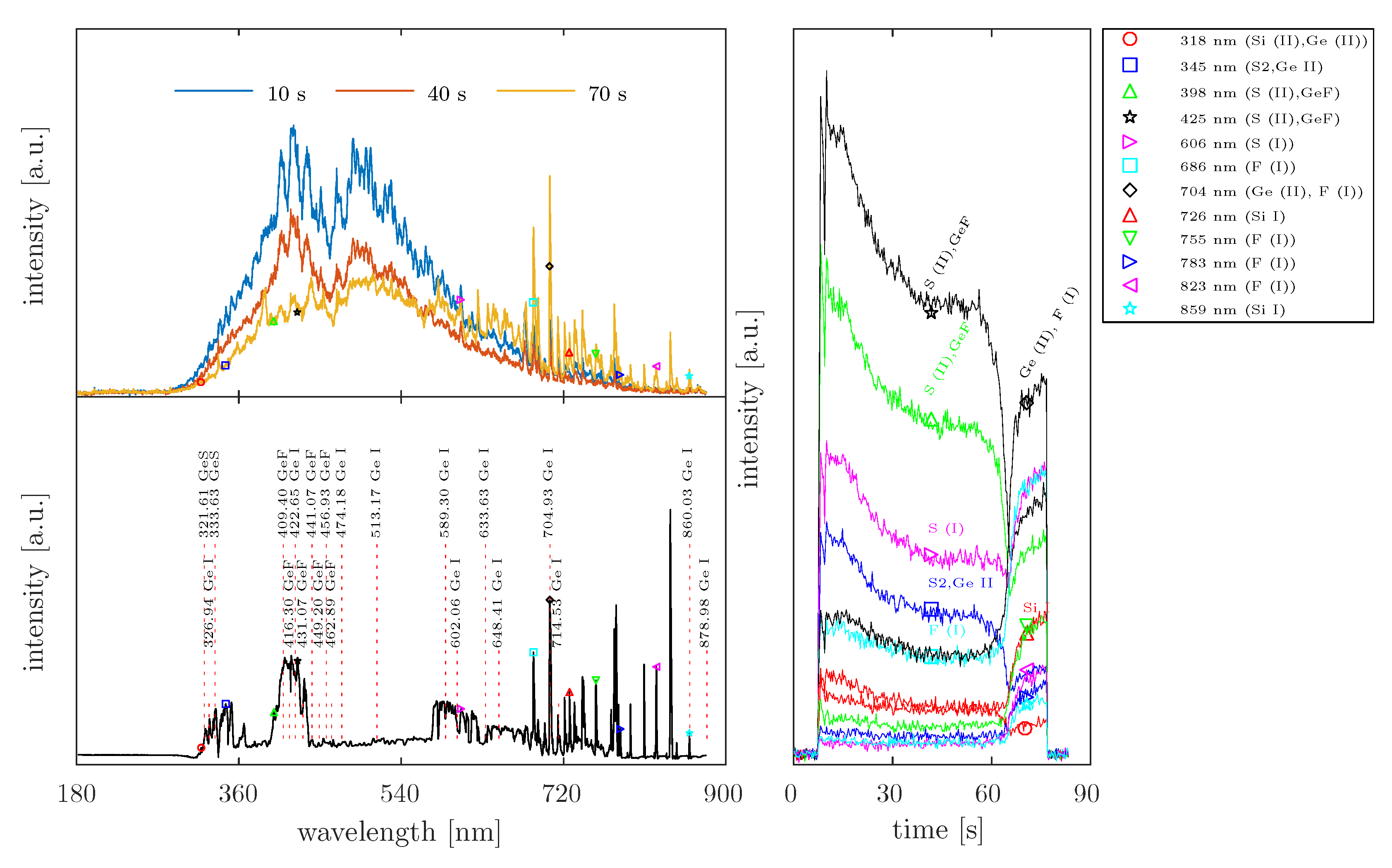When considering the intensity variation in the Fluorine emission (686 nm, 755 nm, and 823 nm), an increase in intensities is only observed after the complete removal of Ge. The peak at 704 nm, which was assigned to both the plasma species Germanium and Fluorine, shows an equivalent temporal intensity behavior to the other emission lines associated with Fluorine. Based on this background, the emission of Germanium at this position would be excluded, which disagrees with the findings in the database entries. This aspect is not interpreted in the present study. In addition, a complete assignment of the emission lines found to plasma species is not attempted, because in this study, the OES data sets were used exclusively to test the developed Method of Spectral Redundancy Reduction.

5. Discussion

Although our MSRR is based on spectral clustering approaches, it differs in various aspects from other methods used for the analysis of optical emission spectra. Typically, the Euclidean distance, Pearson correlation matrix, or cosine similarity are used to construct the adjacency matrix [5,8,11]. In contrast, this study demonstrated that these matrices appear unsuitable for analyzing time-resolved emission spectra and that similarity based on sine similarity leads to better results. Similar to what Puggini and Maclone indirectly suggest in their report on anomaly detection by using OES [7], we do not examine the OES data set for similarity but for “un-similarity” between individual wavelengths. The core of the MSRR algorithm is the calculation of Gaussian similarity through an extension of the approach proposed by [11]. Our proposed Algorithm 4 for computing the Gaussian similarity matrix differs from Kong et al.’s method in three aspects. Firstly, the parameter for including neighboring vertices is determined by the graph itself, specifically by the inhomogeneity across the trace of the graph matrix or calculation step 3 of Algorithm 4). Secondly, the edge impact (the divisor in Equation (19)) is determined by the parameter L, which must be larger than K. Thirdly, instead of the collective impact (Equation (19)), the effective impact (Equation (20)) is computed. It is explicitly noted here that parts of the approach were also arbitrarily chosen. The authors fail to mathematically justify why the inhomogeneity across the vertices degrees should define the necessary input parameter for including neighboring vertices. Furthermore, the determination of the edge impact by using a higher number of neighbors than K is also unjustifiable. Rather, this approach proved to be practical during the course of the study and was confirmed during the evaluation of analyzed data sets.

Currently, the MSRR extracts only two clusters, of which only one is evaluated. Similarly to [3,4], with our algorithm, clustering is naturally predetermined, while in the literature cited, the clusters are divided into the time domain before and after reaching the endpoint. Our intention is to divide the data set into clusters of collective behavior and deviating behavior. However, there is a significant difference: the work of Jang et al. [3] and Lee et al. [4] demonstrates, with their approaches to increase the sensitivity of the endpoint signal in the dry structuring of dielectrics (Si₃N₄ and SiO₂), how powerful the modified k-means clustering or the modified Gaussian mixture model is. However, in both cases, the result is a time-resolved validation factor that is very suitable for process control but does not allow for physical interpretations that contribute to process understanding. With our similarly simple basic assumption of the two-group separation of the OES data, we provide the possibility to make statements about relevant plasma species. Our results also show that the clustering of plasma species based on the eigenvector analysis of graph matrices can work, especially for clusters that represent the consumption and generation of plasma species (the intensity decrease and increase in emission lines) (see Figure 6). This is also suggested by the work of Flynn and McLoone [5], who demonstrated the feasibility of grouping emission lines into more than just two clusters by using “Max Separation Clustering”. However, the authors clearly show that the clustering of emission lines can be strongly disturbed by the effect of noise. To ensure clustering, they reduce the size of the input data set by input channels with a too-high signal-to-noise ratio, but this eliminates the spectral data of the plasma, which can lead to information loss. Generally, the authors of [5] treat the found clusters similarly to the principal components of a PCA. In their report, clustering is solely motivated by the effective representation of patterns through a small number of representative variables, whereas our approach directly uses the methods of (spectral) clustering to ”display” anomalies on the scale of the origin data, thereby ensuring that the result remains physically interpretable even after data reduction, which we demonstrated based on the species assignment of various reactive-ion-etching processes.

In general, according to our research, the methods for reducing the OES data of reactive-ion-etching processes have been primarily used for anomaly detection [7,13] or improved endpoint detection [14,15,16] for more than 10 years and have been continuously optimized. The aim of the methods presented in this work is to address the fundamental nature of the challenges prevailing in reactive-ion-etching processes. In particular, from the perspective of the scientific community interested in reactive etching processes, an optimized endpoint signal without clear physical meaning is not satisfactory. Therefore, ongoing investigations focus on the time-resolved application of the MSRR to evaluate whether a “time-resolved reduced spectrum” similar to that presented in [3,4,17] can be used as a “real-time endpoint control” with increased sensitivity. In contrast to the literature listed here, the advantage would be that the calculated endpoint signal can be directly assigned to specific plasma species.

Furthermore, some methods of optical emission spectra analysis demonstrate the possibility of visualizing the well-known conditioning effect in plasma processing. However, this seems to happen currently at a very abstract level by using a value called “anomaly score” [7,13]. From the perspective of the plasma physics of reactive-ion-etching processes, this type of visualization may provide limited insights. By evaluating the totality of the time-resolved emission spectrum with the proposed method and assuming that the reduced spectra at constant process conditions should not differ with multiple process execution, further investigations will examine if the Method of Spectral Redundancy Reduction—more concretely, the reduced spectrum—can also serve as an instrument for the inspection of the conditioning of the process chamber.

6. Conclusions

In this study, we developed a method based on spectral clustering for the evaluation and analysis of optical emission spectra in reactive-ion-etching processes. Instead of conventional spectral clustering, in which eigenvectors are mainly used for clustering via k-means, our method deals directly with the “display potential” of the eigenvectors of a calculated graph matrix. We showed that the eigenvectors of the underlying adjacency matrix with values of sinus similarity return eigenvectors that best display the emission lines deviating from the collective behavior. The algorithm uses an advanced method to calculate Gaussian similarity, and we further demonstrated that the result is less dependent on the input parameters compared to the other known methods in the literature.

The Method of Spectral Redundancy Reduction calculates a reduced spectrum from a time-resolved optical emission spectrum. The peaks of the spectrum correspond exactly to those that differ from the collective behavior of the entire spectrum, which is why they are referred to as the relevant emission lines of a process.

References

1. Shadmehr, R.; Angell, D.; Chou, P.B.; Oehrlein, G.S.; Jaffe, R.S. Principal Component Analysis of Optical Emission Spectroscopy and Mass Spectrometry: Application to Reactive Ion Etch Process Parameter Estimation Using Neural Networks. J. Electrochem. Soc. 1992, 139, 907. [Google Scholar] [CrossRef]
2. Park, J.H.; Cho, J.H.; Yoon, J.S.; Song, J.H. Machine Learning Prediction of Electron Density and Temperature from Optical Emission Spectroscopy in Nitrogen Plasma. Coatings 2021, 11, 1221. [Google Scholar] [CrossRef]
3. Jang, H.; Lee, H.; Lee, H.; Kim, C.K.; Chae, H. Sensitivity Enhancement of Dielectric Plasma Etching Endpoint Detection by Optical Emission Spectra With Modified K -Means Cluster Analysis. IEEE Trans. Semicond. Manuf. 2017, 30, 17–22. [Google Scholar] [CrossRef]
4. Lee, S.; Jang, H.; Kim, Y.; Kim, S.J.; Chae, H. Sensitivity Enhancement of SiO2 Plasma Etching Endpoint Detection Using Modified Gaussian Mixture Model. IEEE Trans. Semicond. Manuf. 2020, 33, 252–257. [Google Scholar] [CrossRef]
5. Flynn, B.; McLoone, S. Max Separation Clustering for Feature Extraction From Optical Emission Spectroscopy Data. IEEE Trans. Semicond. Manuf. 2011, 24, 480–488. [Google Scholar] [CrossRef]
6. Yang, J.; McArdle, C.; Daniels, S. Dimension Reduction of Multivariable Optical Emission Spectrometer Datasets for Industrial Plasma Processes. Sensors 2014, 14, 52–67. [Google Scholar] [CrossRef] [PubMed]
7. Puggini, L.; McLoone, S. Feature Selection for Anomaly Detection Using Optical Emission Spectroscopy. IFAC-PapersOnLine 2016, 49, 132–137. [Google Scholar] [CrossRef]
8. von Luxburg, U. A tutorial on spectral clustering. Stat. Comput. 2007, 17, 395–416. [Google Scholar] [CrossRef]
9. Mohar, B. Some applications of Laplace eigenvalues of graphs. In Graph Symmetry: Algebraic Methods and Applications; Springer: Dordrecht, The Netherlands, 1997; pp. 225–275. [Google Scholar] [CrossRef]
10. Zelnik-Manor, L.; Perona, P. Self-Tuning Spectral Clustering. In Advances in Neural Information Processing Systems; MIT Press: Cambridge, MA, USA, 2005; pp. 1601–1608. [Google Scholar]
11. Kong, W.; Hu, S.; Zhang, J.; Dai, G. Robust and smart spectral clustering from normalized cut. Neural Comput. Appl. 2013, 23, 1503–1512. [Google Scholar] [CrossRef]
12. Kramida, A.; Ralchenko, Y.; Reader, J.; NIST ASD Team. NIST Atomic Spectra Database (ver. 5.9); National Institute of Standards and Technology: Gaithersburg, MD, USA, 2021. Available online: https://physics.nist.gov/asd (accessed on 26 November 2021).
13. Puggini, L.; McLoone, S. An enhanced variable selection and Isolation Forest based methodology for anomaly detection with OES data. Eng. Appl. Artif. Intell. 2018, 67, 126–135. [Google Scholar] [CrossRef]
14. Zakour, S.B.; Taleb, H. Shift Endpoint Trace Selection Algorithm and Wavelet Analysis to Detect the Endpoint Using Optical Emission Spectroscopy. Photonic Sens. 2016, 6, 158–168. [Google Scholar] [CrossRef]
15. Kyounghoon, H.; Kun, J.P.; Heeyeop, C.; En, S.Y. Modified PCA algorithm for the end point monitoring of the small open area plasma etching process using the whole optical emission spectra. In Proceedings of the ICCAS 2007—International Conference on Control, Automation and Systems, Seoul, Republic of Korea, 17–20 October 2007; pp. 869–873. [Google Scholar] [CrossRef]
16. White, D.A.; Goodlin, B.E.; Gower, A.E.; Boning, D.S.; Chen, H.; Sawin, H.H.; Dalton, T.J. Low open-area endpoint detection using a PCA-based T statistic and Q statistic on optical emission spectroscopy measurements. IEEE Trans. Semicond. Manuf. 2000, 13, 193–207. [Google Scholar] [CrossRef]
17. Lee, S.; Choi, H.; Kim, J.; Chae, H. Spectral clustering algorithm for real-time endpoint detection of silicon nitride plasma etching. Plasma Process. Polym. 2023, 20, e2200238. [Google Scholar] [CrossRef]
Figure 1. Diagram illustrating the calculation of the collective impact on each individual vertex in the graph.
Plasma 07 00015 g001
Figure 2. Generated test data for the evaluation of the MSRR: (a) the temporal change in the entire emission spectrum; (b) the time course of nonvarying (standard), increasing and decreasing lines; and (c) the corresponding average spectrum with marked increasing (incr.) and decreasing (decr.) positions.
Plasma 07 00015 g002
Figure 3. Artificially generated spectrum for eigenvector analysis of various graph matrices.
Plasma 07 00015 g003
Figure 4. The first 7 eigenvectors of normalized Laplacian matrices are as follows. For the distance matrix (Euclidean norm), cosine similarity, and sine similarity (first, second, and third rows), Gaussian similarity matrices with local scaling parameters were obtained by using Kong’s method. A total of 7 neighboring vertices were used to determine the scaling.
Plasma 07 00015 g004
Figure 5. Influence of the number of neighboring vertices on the eigenvectors of the Gaussian similarity matrix.
Plasma 07 00015 g005
Figure 6. Effect of parameter L on eigenvectors 1 to 6. Starting from the 2nd eigenvector, they represent the embedded information in the test data set.
Plasma 07 00015 g006
Figure 7. Reduced spectra calculated based on Gaussian similarity using the method of Kong et al. In total, 38 % of the set-varying positions (symbolized by a circle) are not detected by this approach.
Plasma 07 00015 g007
Figure 8. Reduced spectra based on the proposed method of calculating the Gaussian similarity. Only 12 % of the set-varying positions (symbolized by a circle) are not detected.
Plasma 07 00015 g008
Figure 9. Comparison of the accuracies of reduced spectra using different underlying Gaussian similarity matrices based on (a) relative information loss, (b) relative deviation, and (c) the relationship between relative deviation and the number of varying columns in the data set. Black circle symbols represent 4 and square red symbols represent the method by Kong et al.
Plasma 07 00015 g009
Figure 10. Effect of the parameter ξ on the reduced spectrum using the example of a TiN-etching process. (Left): The reduced spectra for varying ξ values and the mean spectrum of the process. (Right): The time evolution of detected varying positions. In both diagrams, the symbols connect the time evolution with the corresponding spectral position. Dashed lines indicate no anomalies and were not found in the reduced spectrum.
Plasma 07 00015 g010
Figure 11. Effect of the parameter ξ on the reduced spectrum using the example of a copper-etching process. The parameter ξ does not influence the detection of varying spectral positions.
Plasma 07 00015 g011
Figure 12. Result of the MSRR using the example of platinum structuring. (Left): the original data of the optical emission at three different time points, with the reduced spectrum below and probable plasma species indicated. (Right): the time evolutions of detected peaks. The symbols in both diagrams connect the time evolutions with the spectral position.
Plasma 07 00015 g012
Figure 13. Result of MSRR using OES data of a Germanium patterning process.
Plasma 07 00015 g013
Disclaimer/Publisher’s Note: The statements, opinions and data contained in all publications are solely those of the individual author(s) and contributor(s) and not of MDPI and/or the editor(s). MDPI and/or the editor(s) disclaim responsibility for any injury to people or property resulting from any ideas, methods, instructions or products referred to in the content.