In a number of steps, the most important features of the deformation mechanism under impact conditions will be described and connected. It is assumed that the rubber particle size distribution (PSD) is monodisperse. The ligament sizes are calculated using Wu’s regular cubic stacking equation, thereby assuming that all ligament sizes are equal. The cavitation will be described by the Lazerri–Bucknall energy criterion, whereas the response of the ligament will be described by means of the model first described by Van der Sanden, Meijer and Tervoort (VMT) in 1993 [
11]. In order for this model to describe impact, the VMT equation, which describes the energy balance at failure of a ligament, will have to be adapted to the constitutive behavior at high strain rates and low temperatures.
4.1. The Role and Determination of Surface Energy
Both in the Lazerri–Bucknall energy balance description of the cavitation of the disperse rubber particles and in the description of the fracture strength of the matrix ligaments in the VMT model the surface energy Γ appears. Following the original definition of surface energy by Kramer and Berger [
12,
13]:
where
γ is the Van der Waals surface energy contribution,
Ub is the strength of the covalent C–C bond (i.e., 346 kJ/m
2) and
is the node density of load bearing chains at the time scale and the temperature of the experiment, where the suffix e stands for effective.
de is the point-to-point node distance measured along the chain which is related to
ve via the number of Kuhn segments
nL with length
lk and mass
mK in a chain segment.
The Kuhn segment length is the virtual statistical step length for which a polymer chain can be described as a freely jointed chain. The Kuhn segment length is also a measure for the free space mechanical stiffness of the chain, expressed by the persistence length, which is equal to
lk/2 [
14]. Combination of Equation (1) with Equation (2) shows that Γ ~
scales as
. Σ
e represents the axial density i.e., the number of load bearing chains crossing a mathematical surface which is topologically related to
νe as Σ
e = 1/2
νede.
Equation (2) is, of course, only valid when the chain segment between nodes is sufficiently long to allow for Gaussian statistics to be applied, which is usually the case in polyolefin melts and rubbers. However, with increasing network densities, the number of Kuhn segments may require another statistics to calculate
de. For shorter chain segments, the Porod worm chain model should be adopted [
13]:
where
Le is the contour length of the
Me segment. Clearly Equation (4) reduces to Equation (3) for larger
nL. Therefore, in this work, the Porod model is adopted for all calculations of
de, irrespective of the network density up to a network with shear modulus of 5 MPa, which would make
de smaller than the Kuhn length, which is physically impossible.
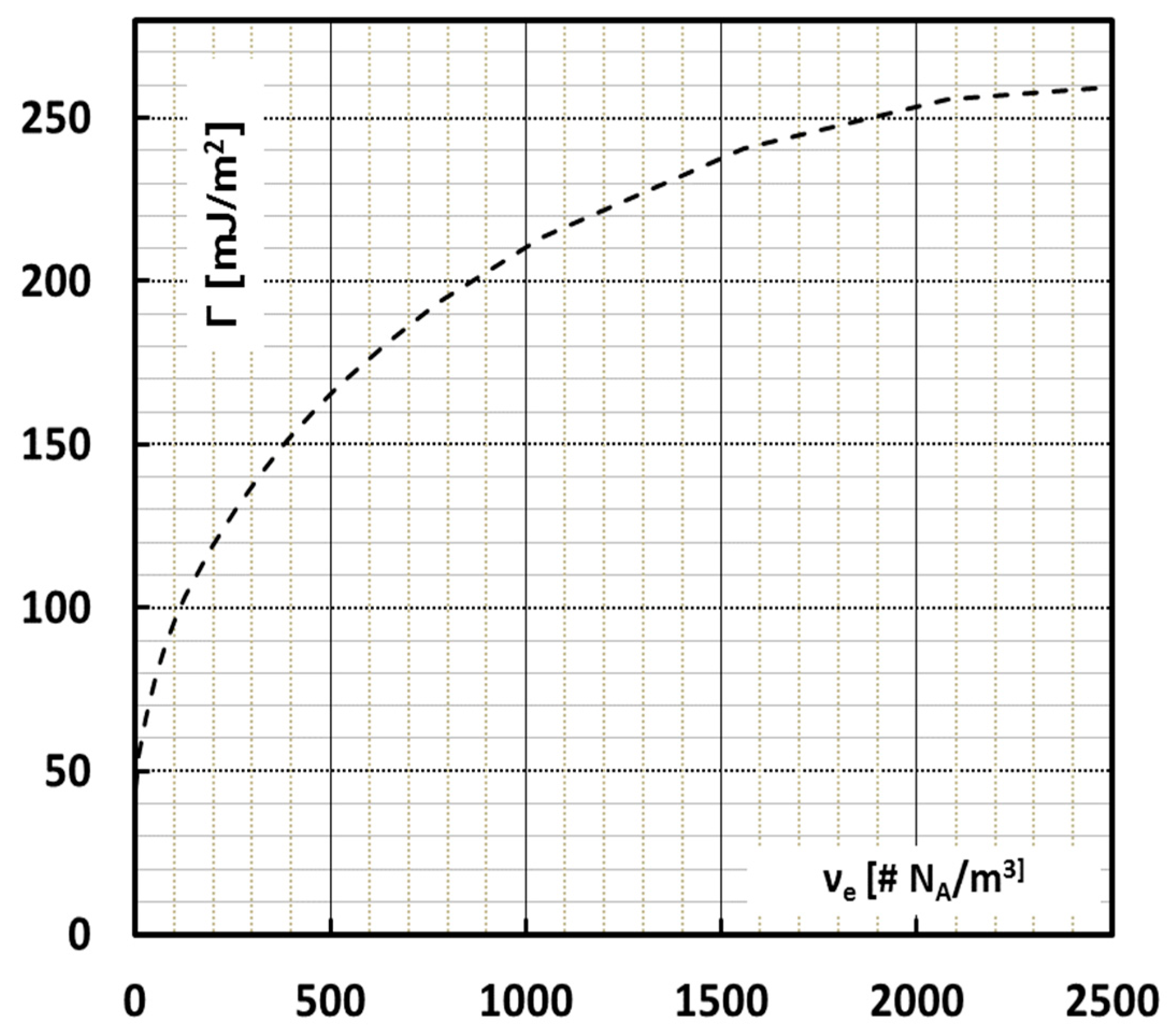
Figure 5 shows the surface energy as a function of the available network density according to Equation (1) taking into account the Porod statistics.
The nodal network with density
can be described by its shear modulus
G′ following rubber elastic theory:
where
A is the network topology factor which we assume to be unity following the work of Fetters [
15]. Equation (5) describes a system of fixed nodes connected by Gaussian chains (i.e., a cross linked rubber) but it is also used to describe time-dependent networks with both fixed and transient nodes [
16]. This rubber elastic description assumes that there is a proportionality of the network shear modulus with temperature and we know that this is not the case. The shear modulus of an uncrosslinked melt entanglement network and the strain hardening modulus in the solid state both decrease with
T and increase with the strain rate which indicates that this network response is mainly enthalpic [
17,
18] and probably mainly caused by segmental and monomeric friction. Notwithstanding this enthalpic nature, Van Melick et al. found that in glassy polymers there is still a proportionality of the strain hardening modulus with the melt entanglement density with a negative linear T dependence, which scales with the yield stress [
19].
The craze microstructure at the time of failure in a slow crack growth process and the time of failure at a given stress in such an experiment have recently been shown to be determined by the strain hardening modulus, determined above the alfa transition [
20]. A practical way of representing the surface energy is therefore via its proportionality with the network shear modulus
G′:
where
ρam is the amorphous density and
mk is the mass of one Kuhn segment. Notice that when the shear modulus vanishes, the surface energy reduces to the Van der Waals value
γ indicative of disentanglement crazing at low strain rates and high
T [
12].
Physical validity of this surface energy concept can be derived from comparison with available experiments and estimations. In Kramer and Berger’s work on craze propagation in amorphous polymers, the value for Γ is taken from the rubber plateau modulus [
12]. This is justified because the mechanically activated continuum at the craze tip is actually in a mechanically liquefied state, comparable to the melt. For polystyrene, this leads to a total surface energy of 0.080 J/m
2, assuming a plateau modulus of 0.20 MPa and a Van der Waals surface energy of 0.04 J/m
2. In that same work, also a strain rate or a temperature dependence of the network density and hence of Γ is assumed in order to describe the transition from scission crazing to disentanglement crazing as a thermally activated process of chain slip.
4.2. The Solid State Surface Energy in Impact Conditions
For the description of the surface energy in the semi-crystalline solid state at short time scales and low T we need to know the number of chains that can be loaded effectively and broken in the course of the surface creation process. There are some obvious Gedankenexperiment-like upper limits to that value; for example, if one were to fracture all chains aligned in a crystal one would have to muster 1.57 J/m
2 for an orthorhombic Polyethylene crystal and for Polypropylene in the monoclinic α phase this would be 0.840 J/m
2. Another upper bound estimate comes from following Huang and Brown’s argument [
21] that in an isotropical amorphous phase, geometrically, one third of the molecular stems are sufficiently oriented and assuming that no slip is possible for all these chains, 30% of that upper bound crystalline surface energy is available, i.e., 253 mJ/m
2 for PP. A lower bound estimate finally would be to take the entanglement density at the rubber plateau
G′ =
GN0 which leads to a value of 0.107 J/m
2.
There are not many experiments that try to relate the fracture stress to the available load-bearing surface (potential surface energy). This surface fraction of tie molecules in polyethylene has been estimated by Brown and Ward, in their famous fracture experiment at 90 K [
22] on polyethylenes. They find up to 23% of surface to be effectively load bearing during the fracture test, which leads us to an estimate of 0.361 J/m
2, in PE. For PP the equivalent estimate would be 0.196 J/ m
2. This compares well with the above estimates.
An experimental attempt to estimate the surface energy from Griffith’s fracture mechanics [
1] approach leads to surface energies, three to four orders of magnitude too large. When one assumes that the critical stress intensity K
1c of iPP lays typically around 3.3 MPam
1/2, Griffith’s theory leads to a surface energy of 5 kJ/m
2. This huge discrepancy is attributed to volume plasticity contributions, typical for a fracture mechanics test, which was exactly what Brown and Ward tried to avoid in their experiment [
22].
It is clear that the surface energy needed to fracture a semicrystalline polymer will be determined by the number of chains that can be loaded and broken in an impact experiment and that number will for impact conditions be higher than the rubber plateau network. We surmise that a valid measure for that number of chains, Σ
e is the solid state strain-hardening modulus [
5], following the work of Haward [
23,
24] and Duffo et al. [
25]. For longer time scales, like in slow crack growth processes, the contribution of the crystal phase will be transient and the network will be limited to a number in the neighborhood of the plateau modulus, with typical shear moduli of the order of 0.5–1.5 MPa. For shorter time-scale processes such as impact at low temperatures, the crystalline phase will function as a robust restraint for the chain segments to slip and virtually all the available nodes will act as fixed nodes. The strain-hardening modulus of solid iPP in the α phase varies from 0.46 MPa at 110 °C to 4.6 MPa at room temperature [
25]. This would indicate that, going from slow (high
T) to fast deformation (low
T) processes, the number of chains loaded may increase a decade or even more. Of course one should be aware that in this transition the material goes from a rubber-like state to a heterogeneous semicrystalline material with some strain localisation caused by the crystals, both in the isotropic regime around yield as in the strain hardening. The working hypothesis we adopt here is that, notwithstanding varying tractability of the crystals, the material can still be considered to form a rubber-like continuum where the strain-hardening response is a measure for the number of load bearing molecular stems at the temperature and the strain rate of the experiment. The surface energies calculated from the assumption that the strain hardening modulus is a direct measure of the number load bearing chains between
Gp = 0.46 and 4.6 MPa, range from 0.107 to 0.205 J/m
2 where it was taken into account that there is a physical limit to the network density when the chain segment becomes equal to the Kuhn length. In our set of experiments, Γ then typically lies between 0.170 and 0.205.
The order of magnitude difference in the network density going to higher strain rates and lower temperature can also be rationalized by looking at the ratio between the number of slipping network links and the number of fixed links in a normal tensile experiment, as calculated from a fit with a slip link model [
26,
27,
28] which is typically a factor of 10.
Conclusion of this section is that depending on strain rate and temperature, the network density may vary and consequently the surface energy will also vary leading to a reformulation of Equation (1) to include the rate and temperature dependence:
4.3. Cavitation, the Lazerri–Bucknall Energy Criterion
Provided that the rubber phase is able to build up sufficient elastic energy, the negative hydrostatic stress will cause rubber particles to void prior to shear deformation of the PP matrix, if the yield stress of the remaining ligament happens to be lower than the brittle fracture stress. This can only happen above the glass temperature (
Tg) of the rubber phase; otherwise, the rubber phase will not localize the strain nor build up elastic energy. This
Tg has of course to be adapted for the strain rate of the experiment, for example, the
Tg at 1 Hz (the standard frequency of a dynamic mechanical thermal analysis (DMTA) test) of the rubber phase in rubber-toughened PP lies around −60 °C. In Izod impact tests the rate is equal to a frequency of 3000 Hz, three decades faster than the DMTA
Tg measurement, in a standard time-temperature equivalence shift (7.8 K/decade), and this implies that rubber particle cavitation is limited to about −36 °C in impact. This generally fits the lowest observed ductile temperatures in rubber-toughened PP well [
9].
A lower brittle–ductile transition temperature could be reached if a lower Tg of the rubber phase is achieved. The lowest possible limit would be achieved by the glass temperature of silane rubbers which is around −125 °C in a DMTA measurement, resulting in about −100 °C under impact conditions.
4.4. The Energy Balance Description within the Rubber Particle
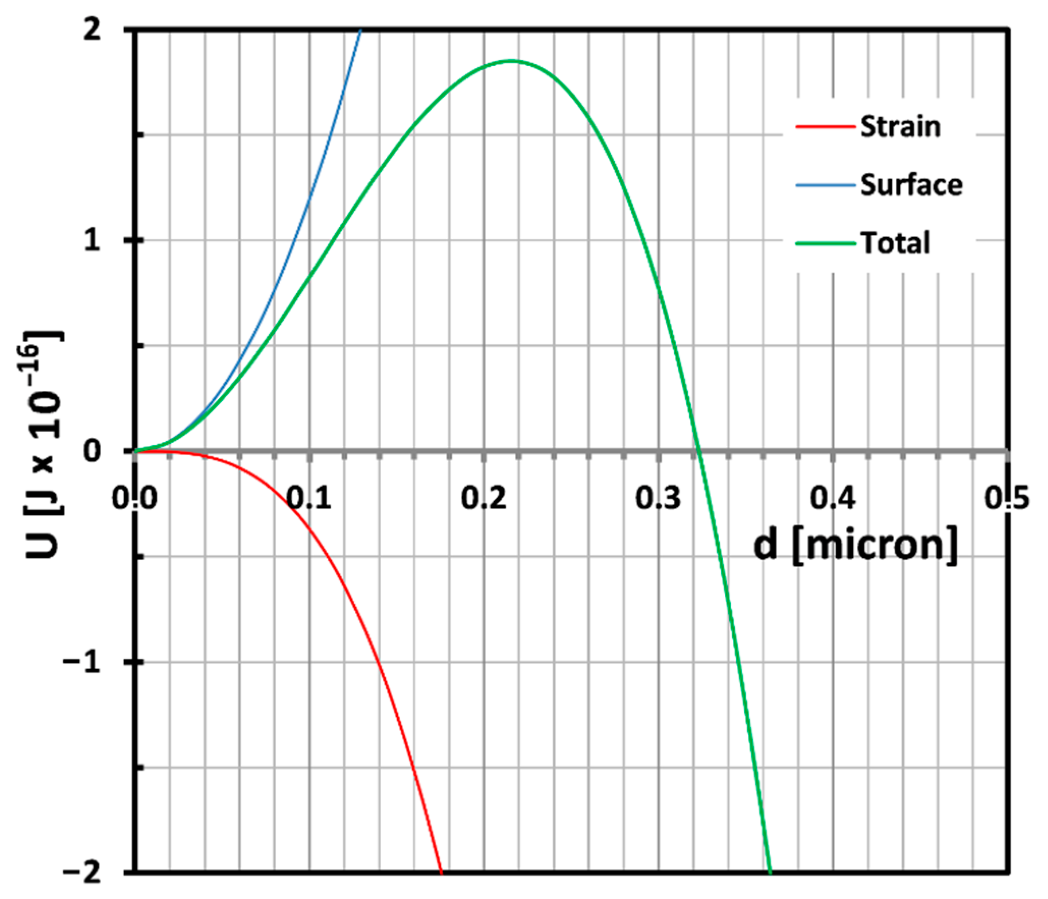
The critical size of the rubber particle
dc for cavitation to occur can be calculated from the cavitation energy balance equation as formulated by Lazzeri and Bucknall [
29]. The energy of a cavitated rubber particle:
where Δ is the volume strain of the rubber particle,
R is the particle radius and
r the cavity radius.
Kr is the bulk modulus of the rubber in the particle. Γ represents the energy required to create surface as defined in Equation (4),
G is the shear modulus of the rubber.
ρ is the density ratio of the rubber phase prior and after cavitation which can to good approximation be considered to be 1.
F(
λf) is a strain function at biaxial failure strain which is typically of the order of unity [
29]. Prior to cavitation (
r = 0) there is only the elastic volume strain energy built up. Equation (7) allows the contributions prior to and after cavitation to be calculated. As stated by Lazzeri and Bucknall the driving force of the cavitation will be lowering of the total energy to a minimum i.e.,
.
They found that minimum to be close to
, i.e., complete vanishing of the accumulated strain energy. One can further assume that the third term in Equation (7) will be balanced by a quasi equal traction on the surrounding matrix [
30], so that the energy balance within the rubber particle before and after cavitation comes down to equating the two first terms of Equation (7). Switching from radia to diameters
d0 = 2R and
di = 2
r and using the relation
di = Δ
1/3d0, the condition for cavitation to occur becomes:
where
Ue and
UΓ are the elastic and the surface energy respectively.
Kr is the bulk modulus of the rubber particle, Δ is the volume strain,
d0 is the initial rubber particle size, and Γ is the surface energy as described by Kramer and Berger’s equation shown in Equation (2).
The energy criterion as shown in Equation (9) has also been formulated by Dompas and Groeninckx [
31].
The critical condition
Utot = 0 yields the critical particle diameter from Equation (9) combined with Equation (6):
This equation shows clearly that the critical particle size depends on the ratio of the shear modulus over the bulk modulus. If easy cavitation is the goal, a high bulk modulus and a low shear modulus are desirable. Typical values for shear moduli and bulk moduli range around 0.5–1.5 MPa and 2–3 GPa respectively. A typical candidate for good cavitation properties in that respect should be a polydimethyl siloxane (PDMS) rubber. The balance described in Equation (9) is plotted in
Figure 6 for a shear modulus of 0.4 MPa and a bulk modulus of 2.5 GPa assuming a volume strain of 0.75% which is a typical value for cavitation occurrence [
32].
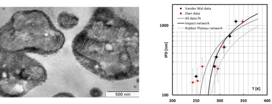
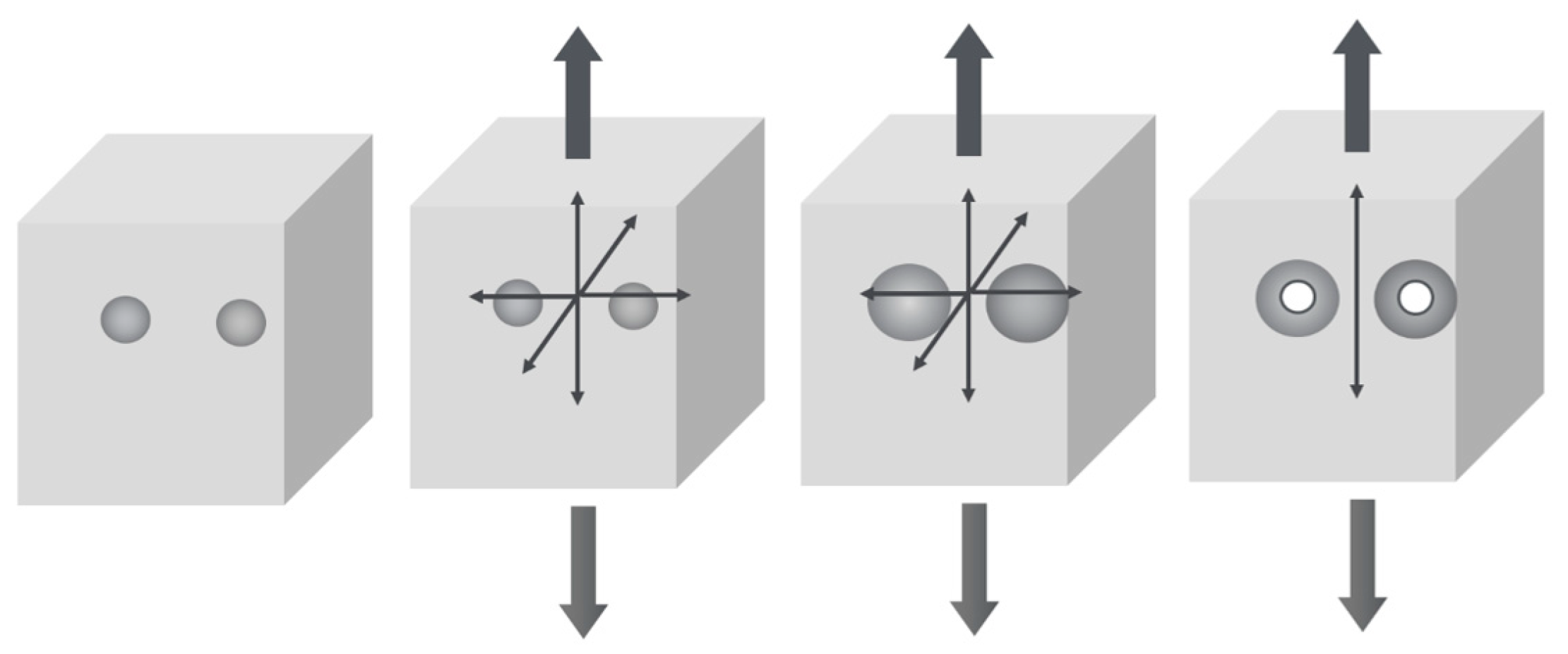
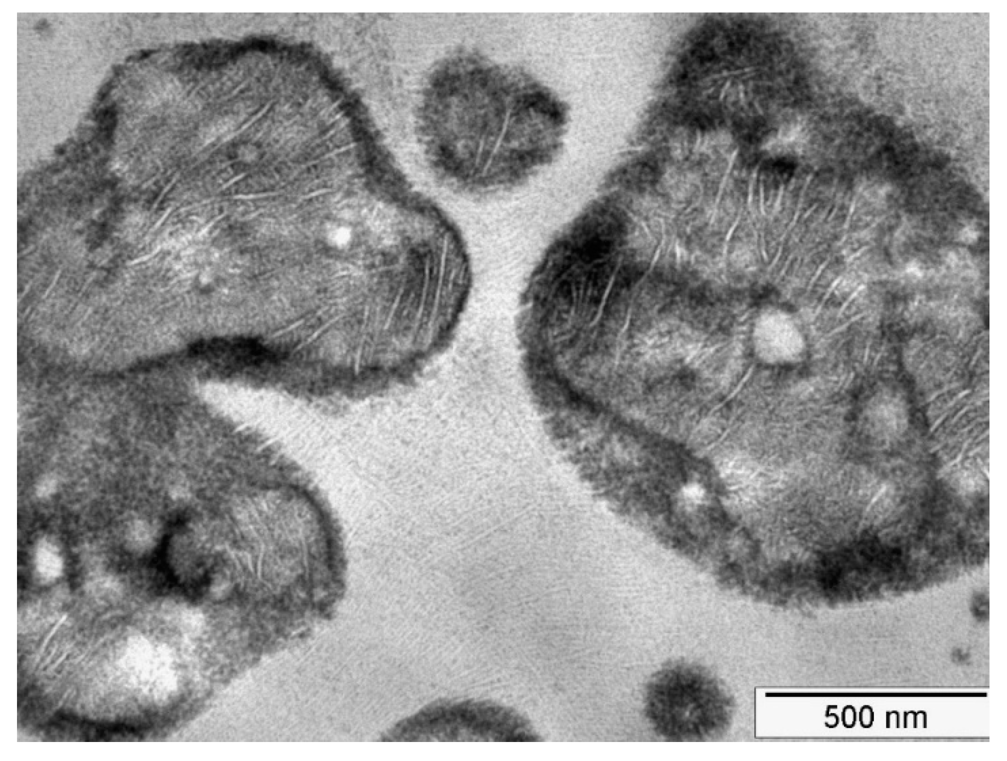
In the present kind of impact-resistant EPR copolymers, the rubber particles are heterogeneous in nature. They are composed of areas with varying composition ranging from PE-rich LLDPE-like areas (featuring the typical morphology of Linear Low Density Polyethylene) to PP-rich occlusions, as shown in the transmission electron microscopy (TEM) image in
Figure 7.
Such a morphology with large differences in local modulus will lead to strain localization in the EPR domains. Because of the low surface energy, these EPR areas will cavitate preferentially as has been shown by means of Scanning Transmission Electron Microscopy computer tomography [
33]. In these images it is also easily seen that the PE and the PP domains do not feature cavitation which is also to be expected in view of the tenfold higher surface energy of these areas. It is assumed that the stored elastic energy that drives the cavitation in these particles will be identical to the energy stored in a homogenous particle.
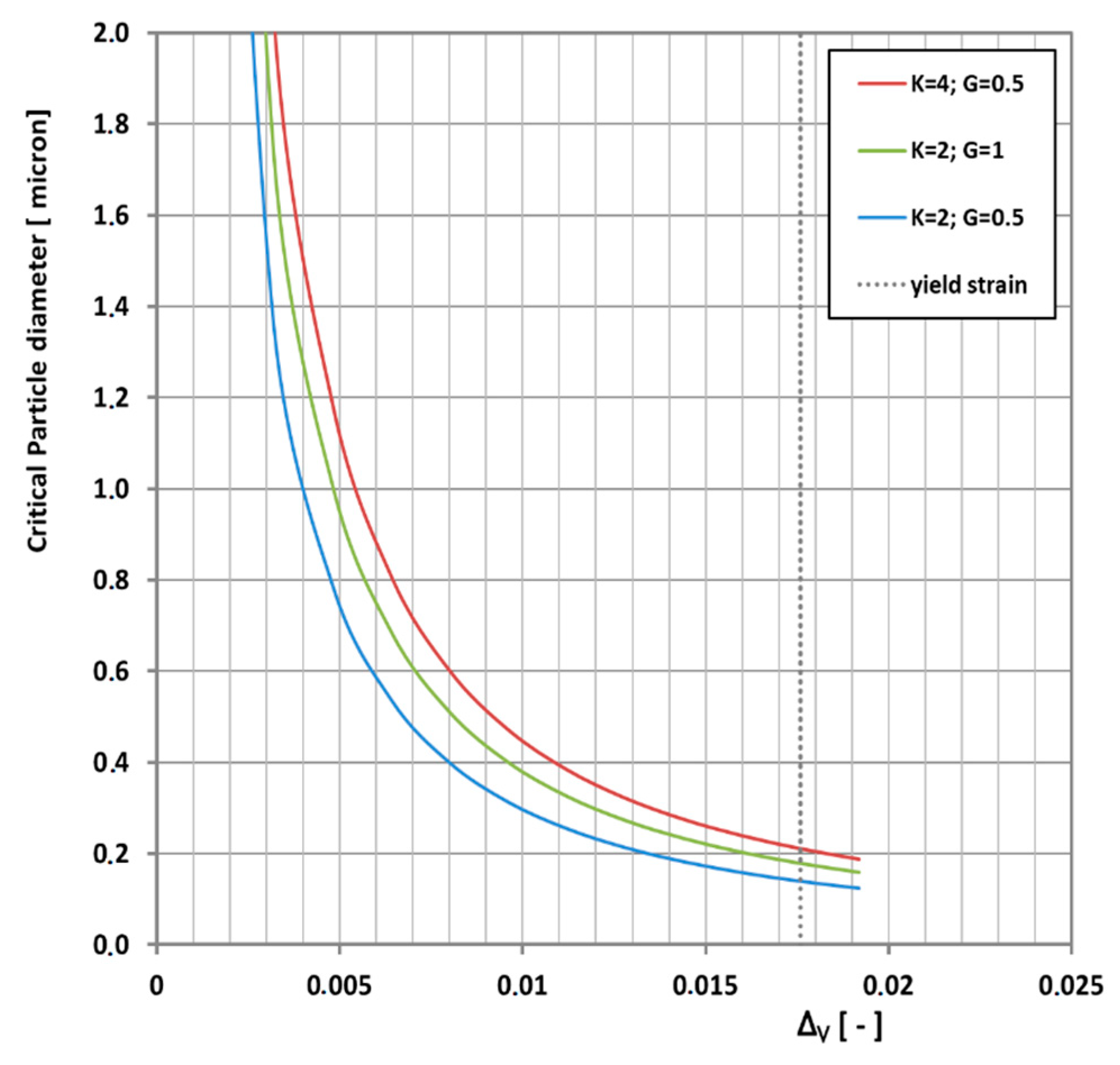
Equation (10) is shown in
Figure 8 for some plausible combinations of bulk and shear moduli.
Increasing the bulk modulus (or density) decreases the critical particle size and increasing the shear modulus increases the critical particle size. Furthermore, it is physically impossible to go beyond yield strain, because when the matrix yields it cannot convey elastic stress to the rubber particles anymore. Particles smaller than the critical particle size will deform affinely with the matrix and will not cavitate. This limit is indicated by the vertical dotted line in
Figure 8.
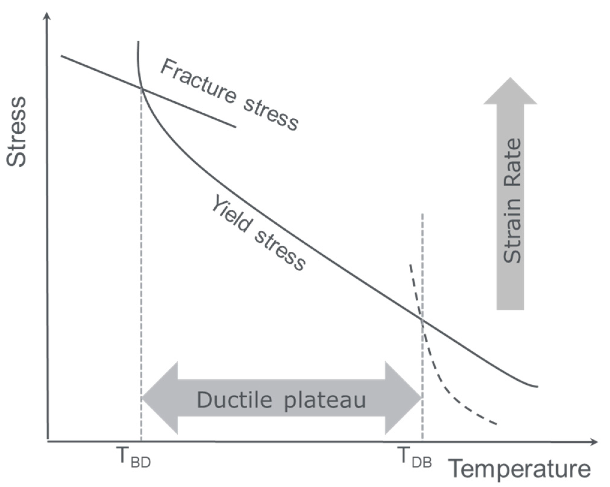
4.5. The Critical Matrix Ligament Thickness for Ductile Failure
After cavitation, the failure mechanism depends on the properties of the matrix ligaments. Two major factors need to be studied: the glass temperature of the matrix PP, and the ligament thickness. An elegant way of calculating the critical matrix ligament thickness for ductile failure is the Van der Sanden, Meier and Tervoort (VMT) criterion [
11]:
This is derived from the energy balance between the available elastic energy within the deforming ligament, represented by the yield stress, and the energy required to create a brittle fracture, represented by Γ. Em is the matrix tensile modulus, is the yield stress of the PP matrix and λmax is the maximum draw ratio of the matrix. The matrix Tg as it will be shown later influences mainly σym, but also Γ, Em and even λmax. Assuming literature melt entanglement densities and normal tensile test conditions at room temperature, the critical ligament size in rubber-toughened PP to achieve toughness is of the order of 2 µm.
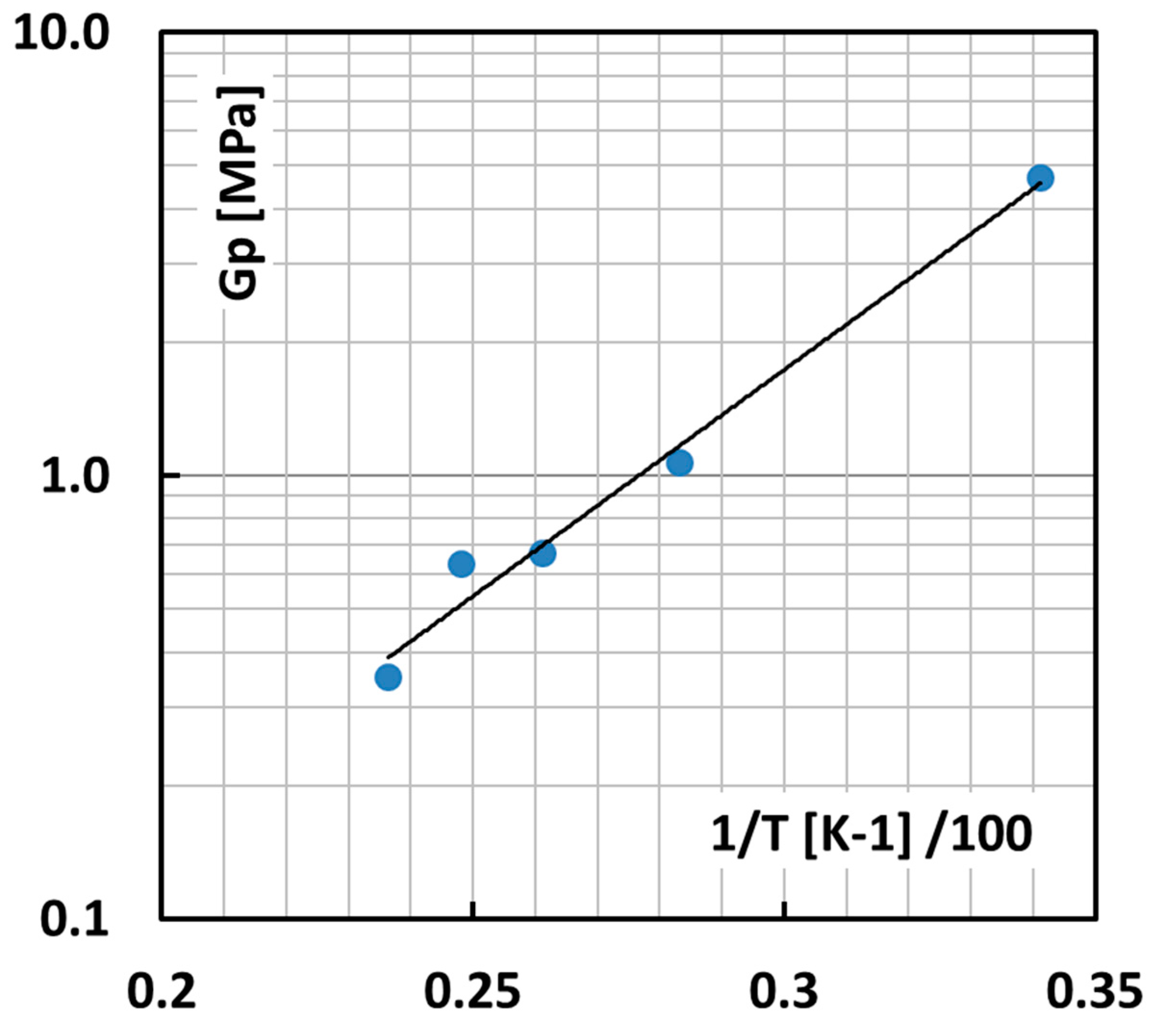
4.7. The Rate and Temperature Dependence of the Network and its Physical Limits
Now that we have realized that the surface energy is determined by the available rate and temperature dependent network density i.e., the available assembly of effective tie molecules, it is necessary to calculate this density. As stated above in
Section 4.2 we assume that this network density is described by the shear modulus of the perceived rubbery response [
5], the strain-hardening modulus
Gp.
The temperature dependence of the strain hardening modulus of isotactic PP has been measured very accurately [
25].
This leaves us with a useful experimental range for the T dependence of the apparent node density in the solid state between room temperature (RT) and 150 °C as shown in
Figure 9 as a log
G′ versus 1/T plot.
The straight extrapolation of the line in
Figure 9 to low T leads eventually to non-physically dense networks with shear moduli far beyond 5 MPa, meaning contour lengths tend to become smaller than the Kuhn length. In this case, it is assumed that the contour length is at least equal to the Kuhn length and consequently
nL = 1 and
λmax = 1. The surface energy then reaches a maximum of a very acceptable 0.205 J/m
2.
4.8. Rate and Temperature Dependence of the Matrix Yield Stress
The iPP matrix typically has a
Tg of 273 K and it is possible that the amorphous PP rubber is in its glassy state at the time scale of a typical impact test. Therefore, it is important to know the influence of the bulk
Tg on the yield stress of iPP. To this end, the literature was screened for such data and some valid and useful plane stress compression measurements for a very wide strain rate range from Okereke et al. [
34] was found. Since the iPP matrix ligaments are tensile loaded in the direction of the applied stress, the compression tests of Okereke et al. need to renormalized to tensile data. Such tensile data were obtained by Van Erp et al. [
35]. As usual the tensile values are lower. This is attributed to two major causes; the first is the opposite sign of the hydrostatic stress in a compression test as compared to a tensile test. This has already been investigated by Mears et al. [
36] who investigated the effect of hydrostatic pressure on both PE and iPP. Kanters et al. [
37] demonstrated how large the hydrostatic effect can be and explains that it can depend on the crystallinity and processing conditions. A second important reason is the friction with the compression plates, which is expected to increase linearly with strain rate, i.e., the ratio between the compression and the tensile value of the yield stress must be constant. However, in sound experiments this friction contribution should be reduced to negligible values, especially at the yield stress where the strain is still quite low.
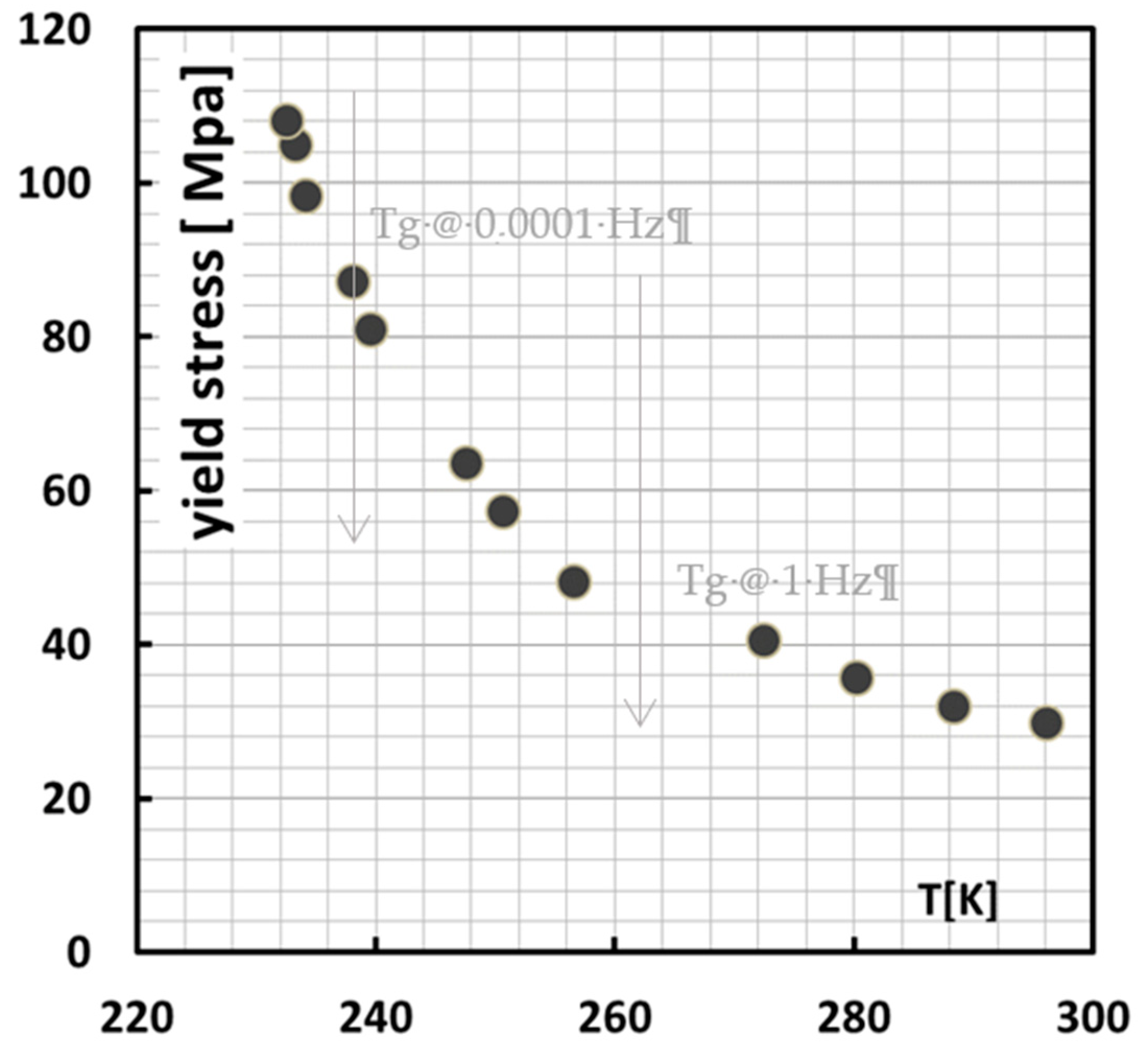
Neglecting friction contributions, an average ratio between compression yield stress and tensile yield stress of 1.38 was observed and applied to transform the compression data to tensile data as it is shown in
Figure 10. This way an estimate of the high strain rate tensile behavior of an iPP matrix ligament is obtained. A note of caution may be necessary here, since our renormalisation implicitly assumes that the processing conditions for both data sets are comparable, which might not have been the case.
Assuming a t,T shift factor of 7.8 K/decade, which is quite common for all t,T shifts in polymers [
38] for creep and yield, this rate dependence can be calculated into a T dependence. The reference rate is taken at the lowest rate, i.e., 0.0001 Hz as is shown in
Figure 11. From RT, for example, it would then take, starting at the lowest test rate, ~3–4 decades to attain
Tg. This would situate the
Tg at around 1–10 Hz, which is what the grey arrow in
Figure 11 suggests, where indeed an extra rate-dependent regime kicks in.
What
Figure 10 and
Figure 11 also suggest is that this strain rate/temperature dependence beyond
Tg is not typically an Eyring process, which would imply a straight line in log (t), but rather a curved Williams Landel Ferry (WLF)-type dependence [
38].
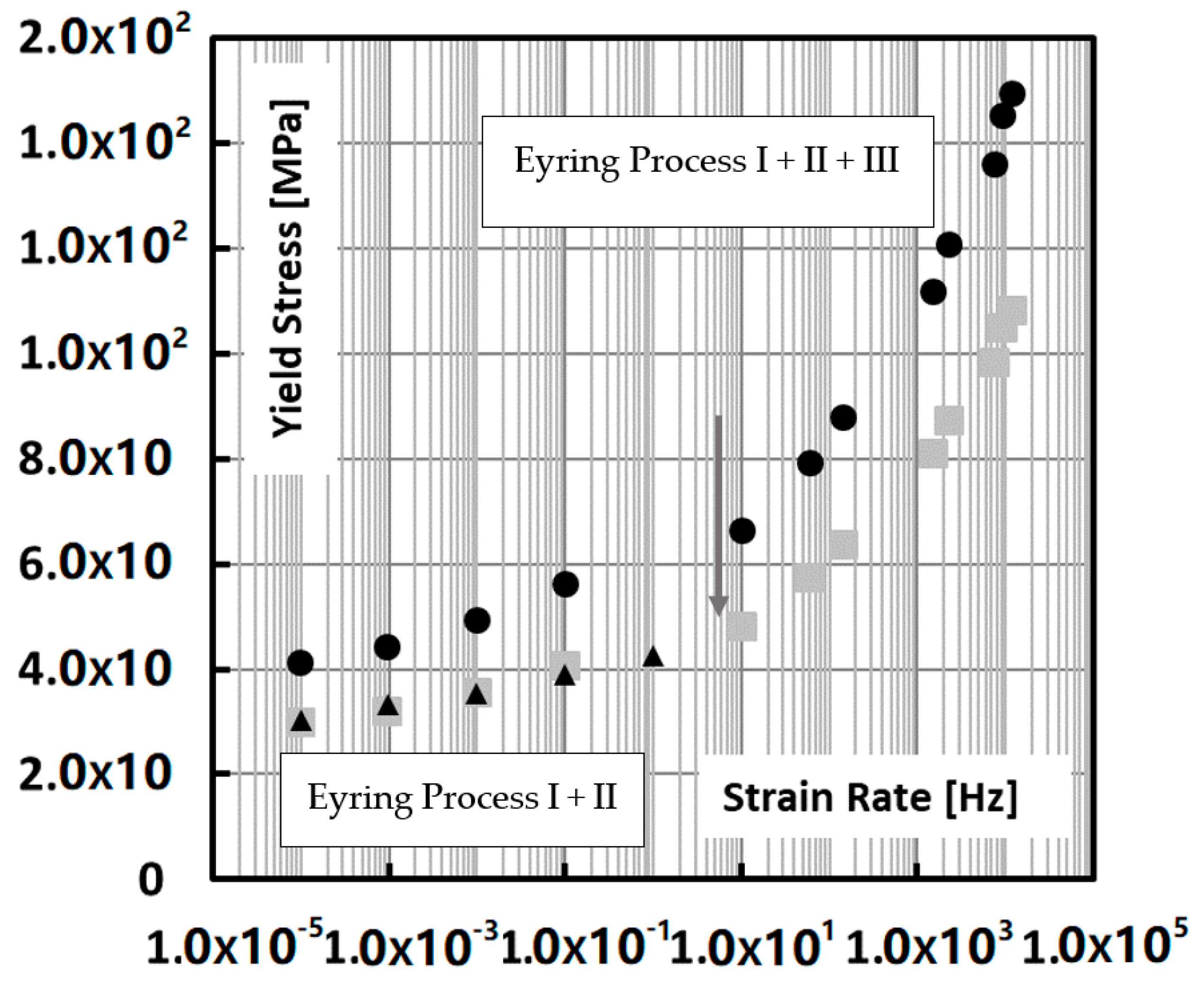
At this point, it is also meaningful to look closer into the work of Van Erp who analysed the rate dependence of polypropylenes in terms of the Ree–Eyring activated flow model [
35]. Generally two Eyring rate regimes are encountered, i.e., process I (low strain rates, high temperatures) and process II that kicks in on top of process I at increased strain rates and lower temperatures. In the range of the Okereke data, there appears to be a third relaxation process on top of process II, most probably caused by the vitrification of the amorphous phase. This third relaxation process has also been confirmed by Caelers et al. in their research on the differences in the creep response of iPP polymorphs [
39].
The present data for the constitutive behavior of isotactic polypropylene shown in
Figure 10 and
Figure 11 are used to calculate the yield stress by inter- or extrapolation of the properly temperature or rate shifted data. However, there is a hard physical limit to this extrapolation in that the estimated yield stress should never exceed the true fracture stress which is typically 250 MPa. This limit is set as a threshold value in the in the calculation of the critical ligaments thickness.
4.9. The Rate and Temperature-Dependent Van der Sanden, Meijer and Tervoort (VMT) Equation for Impact
With the yield stress, drawability and the surface energy dependency on rate and temperature made explicit we are able to fill in the rate and temperature-dependent VMT equation:
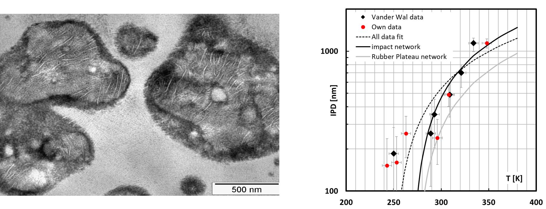
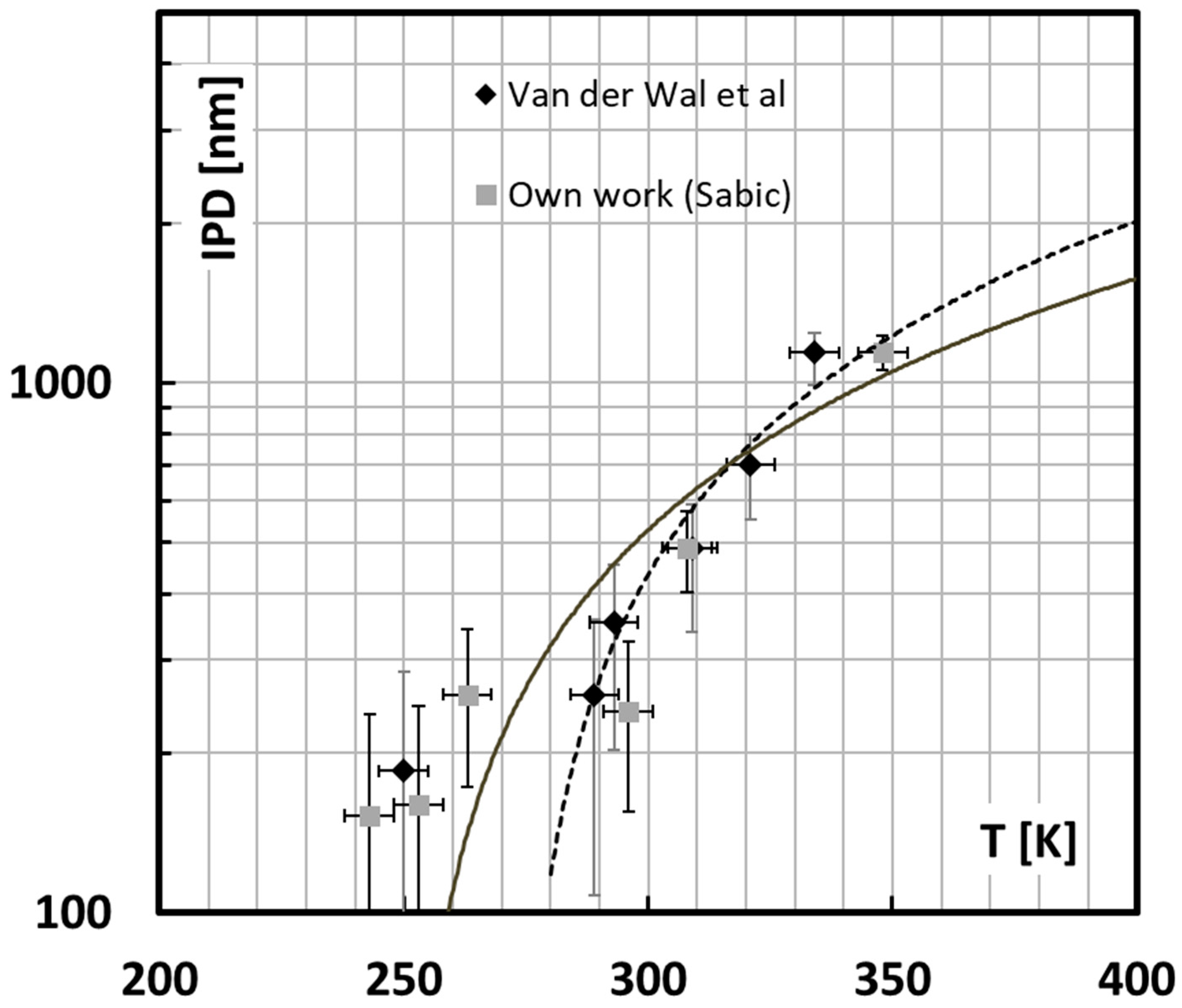
It becomes now possible to use Equation (13), respecting the physical limits of the network density and the yield stress to interpret the available experimental data from Van der Wal’s dataset [
6,
7,
8,
9,
10] and from our own work, shown in
Figure 12. For this calculation it is assumed that the rubber particles are monodisperse and stacked according to a cubic stacking scheme so that all matrix ligaments have the same size. One can then plot the critical interparticle distance as a function of the brittle ductile transition temperature and compare it to these experiments as shown in
Figure 13.
In view of the relative simplicity of the model and the assumptions on the morphological analysis, this is a very satisfying result. The overall trend of the observations is followed albeit the model predicts a much smaller critical interparticle distance than the observations reveal for high rubber content. This is because in a real blend the heterogeneous spatial distribution allows much smaller interparticle distances than the average calculated from the blend morphology especially at high rubber content.
In a next stage it becomes plausible to investigate possible gains in toughness from adapting the morphology according to this simplified model.
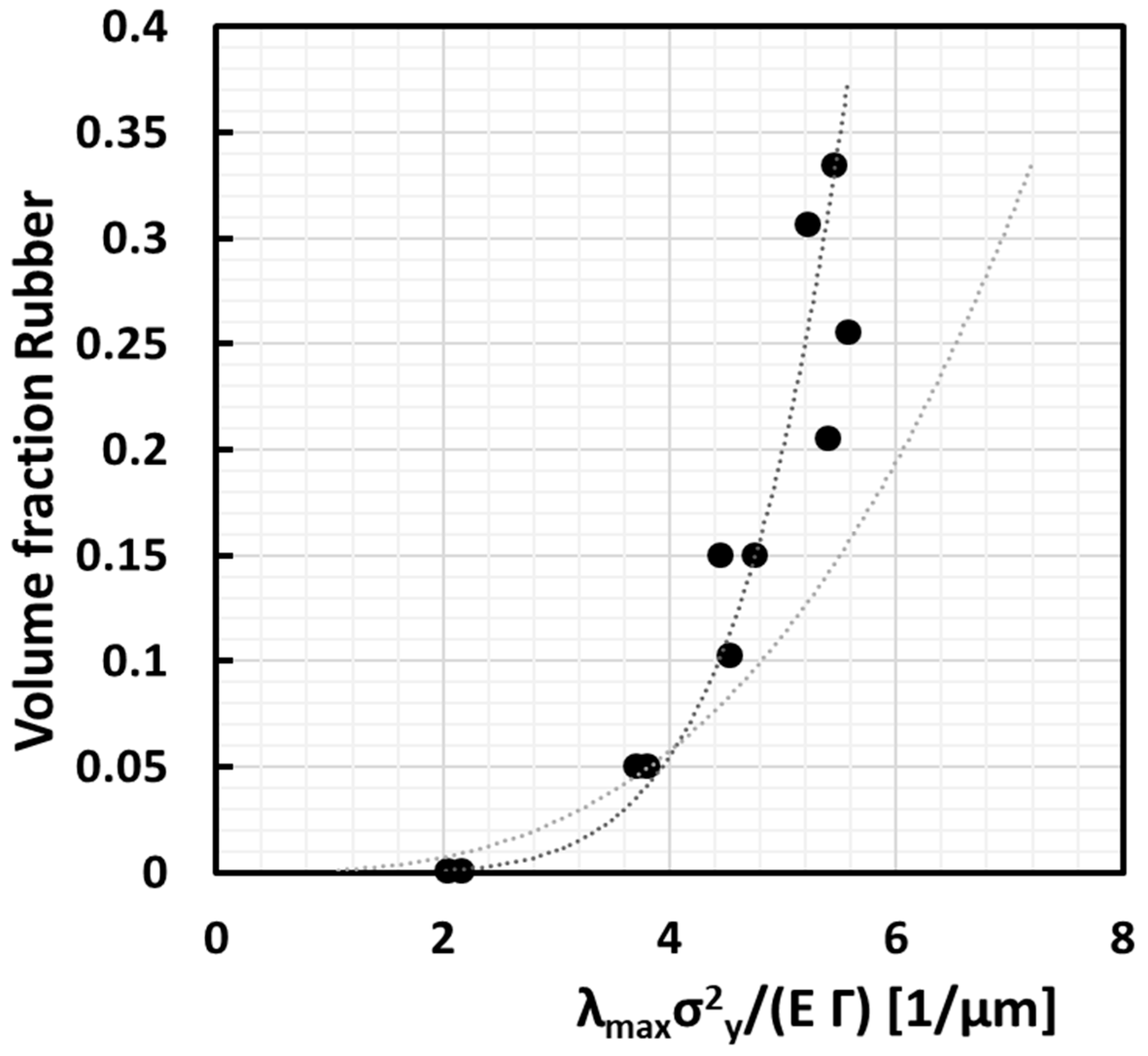
4.10. Effectivity of Rubber Dispersion
Combination of the Lazerri–Bucknall energy criterion of Equation (9), assuming a cubic stacking of monodisperse particles from Equation (1), with the VMT model of Equation (12) taking <
d> =
d0c allows to single out the volume fraction of rubber
φr written to first order as a proportionality with
, which is proportional with the inverse critical ligament thickness
IDc.
where it is assumed that the volume expansion at cavitation, the bulk modulus and the surface energy of the rubber are constant observables.
Figure 13 shows this ideal proportionality (grey curve) compared with the experimental data (black curve). The final fit looks more than good with the exception that the black curve increases with a power higher than 3, i.e., 5.3. This may be attributed to the fact that actually a lot more rubber is needed whenever the distribution deviates from the ideal monodisperse and homogeneous distribution. The theoretical achievable limit for a perfect dispersion should follow a third power ideally. It is clear from
Figure 13 that rubber can probably be distributed much more effectively to achieve a given average ligament size. This would allow achieving a much better toughness/stiffness balance because a rubber content of evenly distributed monodisperse rubber particles of 15 vol % could then already lead to the same brittle ductile temperature as the 30 vol % polydisperse case.


