Article

Sliding Mode Observer-Based Fault Detection and Isolation Approach for a Wind Turbine Benchmark

by
Vicente Borja-Jaimes
1,*,
Manuel Adam-Medina
1,
Betty Yolanda López-Zapata
2,
Luis Gerardo Vela Valdés
1,
Luisana Claudio Pachecano
1 and
Eduardo Mael Sánchez Coronado
3
1
Centro Nacional de Investigación y Desarrollo Tecnológico, Interior Internado Palmira s/n Col Palmira, Cuernavaca 62490, Morelos, Mexico
2
Departamento de Mecatrónica, Universidad Politécnica de Chiapas, Tuxtla Gutiérrez 29082, Chiapas, Mexico
3
Departamento de Ingeniería Mecatrónica, Universidad Tecnológioca del Centro de Veracruz, Cuitláhuac 94910, Veracruz, Mexico
*
Author to whom correspondence should be addressed.
Submission received: 15 November 2021 / Revised: 7 December 2021 / Accepted: 8 December 2021 / Published: 28 December 2021

Abstract

:
A fault detection and isolation (FDI) approach based on nonlinear sliding mode observers for a wind turbine model is presented. Problems surrounding pitch and drive train system FDI are addressed. This topic has generated great interest because the early detection of faults in these components allows avoiding irreparable damage in wind turbines. A fault diagnosis strategy using nonlinear sliding mode observer banks is proposed due to its ability to handle model uncertainties and external disturbances. Unlike the reported solutions, the solution approach does not need a priori knowledge of the faults and considers system uncertainty. The robustness to disturbances, uncertainties, and measurement noise is shown in the dynamic of the generated residuals, which is sensible to only one kind of fault. To show the effectiveness of the proposed FDI approach, numerical examples based on a wind turbine benchmark model, considering closed loop applications, are presented.

1. Introduction

Wind energy has been one of the fastest growing renewable energy sources in recent years [1]. Recently, alternative research has emerged, known as hybrid wind and photovoltaic (PV)-based systems, which provide information on the improvements of these two activities together, as described in [2]. Therefore, development of new wind turbines and wind energy conversion systems, to increase the efficiency and reliability of the energy conversion process, has become one of the main activities (and challenges) of the power industry, as well as the design of new approaches for fault diagnosis. From the reliability analysis carried out by leading countries in the production of wind energy, it is known that most of the faults that occur in wind turbines are located in the pitch system, drive train, and the control system [3]. Moreover, other faults that commonly occur are located on input and output sensors of the different subsystems that make up the wind energy conversion system [4].
In addition to their susceptibility to faults, wind turbines present significant control challenges due to the fact that they include several subsystems and due to the non-linear nature of their input [5]. Therefore, there are different approaches that describe the wind turbine model, such as in [6], where a method is proposed to analyze the parameters in the propeller design, such as drag force, lift force, thrust coefficient, power coefficient, and lift coefficient, among others. These mathematical formulations used in the QBlade software were based on the blade element moment (BEM) theory. In the work [7], specific airfoil simulations were performed for wind turbines of less than 1 kW, considering that the nominal wind speed was 8.4 m/s. In the presented simulations, lift and drag coefficients for different angles of attack are compared. Furthermore, a blade design and performance analysis were published in [8], where the main objective was to optimize the number of blades and tip speed ratio. A frequency regulation model for a wind farm and a thermal power plant was established in [9], where the main variable to be controlled was the load frequency of the produced power. To obtain an equivalent model of a wind farm, different wind turbines were compared, computing the gap metrics of 11 models under different operating conditions. One way to avoid wind turbine failures is through early fault detection methods. An FDI-based approach to dynamic systems, where faults can be detected and located, is described in [10]. This is based on data-driven, intelligent, and analytical modeling methods. In the literature, data-based diagnostic systems use multi-sensors that are a set of signals with fusion technology, which allows estimating, combining, and correlating the data obtained from sensors or information sources [11]. In the sense of the use of multi-sensors, but applied to fault diagnosis in engines, there is a proposal using infrared thermal imaging data, and vibration measurements for automatic fault detection [12]. In the multisensory integration to perform FDI in rotating machines, there is work using data fusion and artificial neural networks [13], FDI was also done using learning algorithms limited to rotor faults [14], the latter later proposed another work based on the same fault detection strategy, but on the gearbox [15]. Multi-sensor techniques represent an interesting and novel alternative to perform FDI in wind turbines.
On the other hand, model-based methods for fault diagnosis in wind turbines present good results, such as in [16], where the diagnosis is carried out using Kalman filters for residual generation. The model-based approach is more frequent in the literature than the data-driven approach, since it is possible to use existing mathematical methods based on differential equations to design control approaches based on fault diagnosis for wind turbine systems [17]. The methods proposed in the literature generally use thresholds for the residual values generated by the difference between the outputs of observer banks and the output signals of the system, as shown in [18]. Fault detection in wind turbine systems is reported in [19] and fault diagnosis based on state estimation is presented in [20]; these works describe the detection and isolation of faults in sensors and actuators of reference wind turbines. An approach to detect faults in actuators and sensors of wind turbines using unknown input observers (UIOs), is presented in [21]. Fault detection is carried out using residual signals and fault localization is achieved by estimating states, output signals, and controlled input signals without considering step faults. In [22], an adaptive diagnosis based on an observer is designed to perform FDI in wind turbines. In [23], three different FDD approaches are addressed, in the power train subsystem, in the generator, and in the wind turbine converter. A robust fault estimation scheme is presented in [24], where actuator and sensor faults in the pitch and drive train system are considered. Robustness is achieved by decoupling the faulty dynamics from the system using a series of coordinate transformations. For the non-faulty dynamics, an observed reduced order input is used for state estimation. While for dynamic faults, an accommodation approach based on sliding mode observers is presented. In [25], a wind speed estimator is developed to remedy the inaccuracies in the single point measurement in the WECS gondola by using the discrete Kalman filter to perform the aerodynamic torque estimation and subsequently calculate the effective wind speed. The design procedure, calculation, and estimation procedure are repeated by implementing an extended Kalman filter (EKF). The results of both algorithms are compared by simulation.
Sliding mode designs for observer and/or control are well known for their robustness properties [26]. Therefore, in [27], an approach based on adaptive sliding mode observers in wind turbines is proposed to perform fault diagnosis as part of an adaptive fault tolerant control (AFTC). In this approach, the adaptive sliding mode observer is used to simultaneously detect both the actuator and sensor faults. In the FTC design, model uncertainty and wind speed variations are considered as unknown disturbances. This allows accurate state estimation and reconstruction of the disturbances. However, the proposed scheme does not consider the faults in the pitch and drive train.
From the literature review, it can be observed that, to solve the problem of detecting faults in the pitch system and handling dynamics introduced by faults, most of the authors have presented methods of compensating for the dynamics introduced by faults. However, the main drawback of the methods presented is that a priori knowledge of the magnitude of the faults is required. On the other hand, the problem of the lack of precision in the measurement of the rotor torque has been addressed through estimation approaches, which do not consider the uncertainty present in the estimation and the system itself.
In this work, a benchmark model is used, which consists mainly of three parts: the blade and pitch system, the generator and converter, as well as the drive train, for which a three-bladed horizontal wind turbine coupled to an electric generator with a capacity of 4.8 MW is considered. The model allows proposing faults in the actuators, sensors, and systems in the pitch actuators, the drive train, as well as in the converter system. In addition, it offers the possibility to analyze and study the operation with different types of structures for the detection and localization of faults in the wind turbine model in a more realistic context [28]. A fault diagnosis approach is proposed on this model. The main contribution of this work is the design of a fault diagnosis for the pitch system and the drive train of a wind turbine model-based. The novelty of the proposed approach is that the problem of the dynamics introduced by the faults, and the uncertainty associated with the system, in a simple way, is addressed, and eliminates the need to know a priori the behavior of the faults. Fault detection and isolation is done using the concept of residual signals and fault signatures. For the residual generation, a bank of sliding mode observers is proposed, which are designed to be sensitive only to one type of fault and to be robust to both, the dynamics of the faults and system uncertainty. This is accomplished through proper handling of the observer’s error injection term and a transformation of the model in which the error introduced by the faults and the uncertainty of the system act on the input signal. The results obtained in simulation show the effectiveness of the proposed scheme.
The document is organized as follows: in Section 2 we present the wind turbine model, sliding mode observer design, and FDI scheme based on sliding mode observers, Section 3 describes the results obtained from numeric examples; Section 4 is a discussion about the results analyzed and finally the conclusion is presented.

2. Materials and Methods

2.1. Wind Turbine Model

The nonlinear wind turbine model considered in this paper is the benchmark described in [28]. This benchmark model considers the wind turbine at the system level as shown in Figure 1. This figure shows the interconnection of the subsystems that make up the wind turbine. The input to the system is the wind speed v ω , which causes the turbine blades to rotate. This motion propagates through the rotor at a speed ω r , and a torque τ r . The drive train couples this motion with the shaft of the generator, which rotates at a speed ω g , and has a torque τ g . The generator is in charge of transforming the mechanical energy into electrical energy. The electrical power generated by the system is controlled by modifying the turbine aerodynamics through pitch control or by controlling the rotational speed of the generator (torque control). In either case, the objective of the control system is to track the reference electric power P r e f , or, if not possible at least, to minimize the tracking error. The pitch control block in Figure 1 receives as inputs the measurements of the pitch angle β i , the generator speed ω g , and the generated electrical power P g . The output of the block is the pitch position reference signal β r e f , which will allow the capture of the kinetic energy needed to produce the desired electrical power output. On the other hand, the torque control block has as input the generator speed measurement and the generated electrical power. The controller generates as output the reference torque τ r e f , which will allow us to reach the desired electrical power output.
The mathematical model of each component of the wind turbine shown in Figure 1 is presented in the following lines.

2.1.1. Blade and Pitch Model

This model is a combination of the aerodynamic model and the wind and pitch model. The wind turbine nonlinear aerodynamic model is modeled as a torque acting on the blades. This aerodynamic torque is defined as
τ r ( t ) = 1 2   π ρ R 3 υ ω 2   ( t ) S   ( λ , β )
where S ( λ , β ) is the power coefficient, R is the rotor ratio, ρ is the density of the air, and v w ( t ) is the wind speed.
The hydraulic pitch system is modeled as a second order transfer function
β i ( s ) β r e f ( s ) = ψ 2 s 2 + 2 ζ ψ   s + ψ 2
where β i is the i t h pitch system whose position is measured with two sensors β i , m 1 and β i , m 2 ; β r e f ( t ) is the reference value, ζ is the damping factor, and ψ is the natural frequency.

2.1.2. Drive Train Model

The drive train system is modeled by a simple two-mass model. Therefore, a drive train model can be represented by
J r ω ˙ r ( t ) = τ r ( t ) K dt θ ( H dt F r ) ω r ( t ) + H dt N g ω g ( t ) J g ω ˙ g ( t ) = ( η dt K d t ) N g θ + ( η dt H dt ) N g ω g ( t ) ( ( η dt H d t ) N g 2 + F g ) ω g ( t ) τ g ( t ) θ ˙   ( t ) = ω r ( t ) 1 N g ω g ( t )
where ω r and ω g are the rotor and generator speed, both measured by two sensors ω r , m i and ω g , m i (with i = 1   = 2 ). Moreover, θ denotes the torsion angle of the drive train. τ g and τ r are the converter and aerodynamic torques. J r y J g are the moment of inertia of the low- and high-speed shafts, respectively. F r and F g are the viscous frictions of the low- and high-speed shafts, respectively. K d t . is the torsion stiffness of the drive train, H d t is the torsion damping coefficient of the drive train, N g is the gear ratio and η d t is the efficiency of the drive train.

2.1.3. Generator and Converter Model

The generator and converter dynamics can be modeled by a first–order transfer function:
τ g ( s ) τ g , r e f ( s ) = γ s + γ
where τ g , r e f is the reference value and γ is the cutoff frequency. The power produced by the generator is given by
P g ( t ) = η g ω g ( t ) τ g ( t )
The efficiency of the generator is determined by η g and P g is the power produced by the generator.

2.2. Sliding Mode Observer

The objective of an observer is to estimate the states of a system, which are generally not measurable. In essence, an observer is a mathematical model of the system, which receives the inputs of the system and the estimation error obtained from the difference between the output of the system and the output of the observer himself.
The simplest form of an observer is the Luenberger observer, in which the estimation error is fed back linearly through a gain. However, the Luenberger observer is very sensitive to measurement noise and the success of the estimation is highly dependent on the accuracy of the system model. Therefore, if the model presents some uncertainty, or is affected by external disturbances, the estimation results will be very poor. To overcome this drawback, the design of a type of non-linear observer is proposed, known as a sliding mode observer. This observer shows to be insensitive to parametric variations and presents robustness to disturbances, which represents a great advantage over other types of observers [29]. In particular, in this work, these properties are used to obtain accurate estimates of the measurements made by the sensors, even in the presence of system faults and uncertainty.
To appreciate the properties of the sliding mode observers, namely, their robustness to modeling uncertainties and disturbances, the design considers a system with uncertainty with representation in the state space given by:
x ˙ ( t ) = A x ( t ) + B u ( t ) + D ξ ( t , x , u ) y ( t ) = C x ( t )
where A R n × n , B R n × m , C R p × n , and D R n × q with p q . Assume that the matrices  B ,   C are the full rank and the function ξ : R + × R n × R m R q is unknown, but bounded so that ξ ( t , x , u ) r 1   u + α ( t , y ) and α : R + × R p R + .
Suppose that exits a liner change of coordinates T so that the system can be written as
x ˙ 1 ( t ) = A 11 x 1 ( t ) + A 12 x 2 ( t ) + B 1 u ( t ) x ˙ 2 ( t ) = A 21 x 1 ( t ) + A 22 x 2 ( t ) + B 2 u ( t ) + D 2   ξ   y ( t ) = C x ( t )
where x 1 R ( n p ) ,  x 2 R p , and the matrix A 11 has stable eigenvalues. The observer structure that will be considered can be written in form
  x ^ 1 . ( t ) = A 11 x ^ 1 ( t ) + A 12   x ^ 2 ( t ) + B 1 u ( t ) A 12 e y ( t ) x ^ ˙ 2 ( t ) = A 21 x ^ 1 ( t ) + A 22 x ^ 2 ( t ) + B 2 u ( t ) ( A 22 A 22 s ) e y ( t ) + w   y ^ ( t ) = x ^ 2 ( t )
where A 22 s is a stable design matrix, e y ( t ) = y ^ ( t ) y ( t ) and the discontinuous vector w is defined as
w = { σ D 2 P 2 e y ( t ) P 2 e y ( t )   if   e y 0   0   otherwise  
where P 2 R p × p is a symmetric positive defined Lyapunov matrix for A 22 s .
The scalar σ is chosen so that ξ < σ . If the state estimation error is defined as e 1 ( t ) = x ^ 1 ( t ) x 1 ( t ) , then it is straightforward to show
e ˙ 1 ( t ) = A 11   e 1 ( t ) e ˙ y ( t ) = A 21   e 1 ( t ) + A 22 s   e y ( t ) + w D 2   ξ
It is shown in [30] that the error system Equation (10) is quadratically stable and a sliding motion takes place, forcing e y   ( t ) = 0 in finite time.
If x ^ ( t ) represents the state estimate for x ( t ) and e ( t ) = x ^ ( t ) x ( t ) , it follows that if
G l = T 1 [ A 12 A 22 A 22 s ]   and   G n l = [ D 2 ] T 1 [ 0 I p ]
then the robust observer given in Equation (8) can be written in terms of the original coordinates in the form
x ^ . ( t ) = A x ( t ) + B u ( t ) G l C e ( t ) + G n l w
where the nonlinear function is given by
w = { σ P 2 C e ( t ) P 2 C e ( t )   if   C e 0   0   otherwise
It is important to note that, even when the model considered for the design of the sliding mode observer has an uncertainty term, the dynamics of the observer does not depend on the uncertainty; therefore, the convergence of the observer is achieved even in the presence of uncertainty.
The methodology for the design of the sliding mode observer described in this section is applied in the following sections for the development of fault diagnosis schemes in the pitch and drive train system.

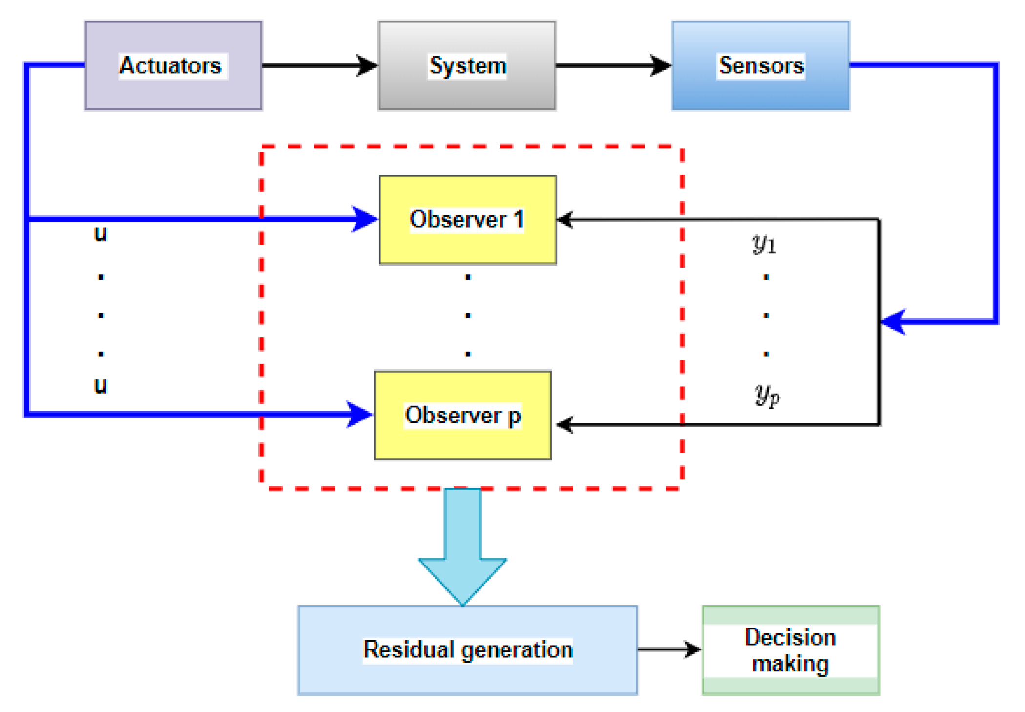
2.3. FDI Scheme Based on Sliding Mode Observers

The principal purpose of the FDI scheme is to generate an alarm when a fault develops in the system and to identify the source and location. To detect and isolate faults on the wind turbine, a model based FDI is proposed. To achieve fault detection and isolation in the model-based approach with the observer-based method, some authors have proposed particular configurations of observer banks. In this work, the proposed scheme is based on the configuration presented in [31], and is shown in Figure 2. In this scheme, a set of observers dedicated to isolate p sensor faults are designed, the proposed configuration allows observer p to use all inputs and only output p. In this way, observer p is sensitive to sensor p faults. The residue generator block generates a set of structured residues from the difference of the measured variables and those estimated by the observer bank. In the decision block, the decision is made to detect the fault if the residual exceeds a predefined threshold.
Since the wind turbine system is subject to modeling uncertainty and unknown disturbance, to achieve the effective fault detection, a robust fault detection scheme is needed. Since the sliding mode techniques are well known for their robustness properties, the bank of the observer is designed using these techniques.
The novelty of the proposed scheme is that it does not require a priori knowledge of the failures and considers the uncertainty of the system. This is achieved by treating the dynamics of the faults in the pitch system and the uncertainty in the estimation of the rotor torque, as coupled disturbances acting on the input signal. Under this condition, it is possible to observe the characteristics of the sliding mode observer. The faults considered in this paper cover the pitch systems and drive train, and these are independent. Therefore, an FDI scheme was designed separately for each one.
The configuration proposed for the development of the fault diagnosis scheme in the pitch system is presented below, considering the general structure described in Figure 2.

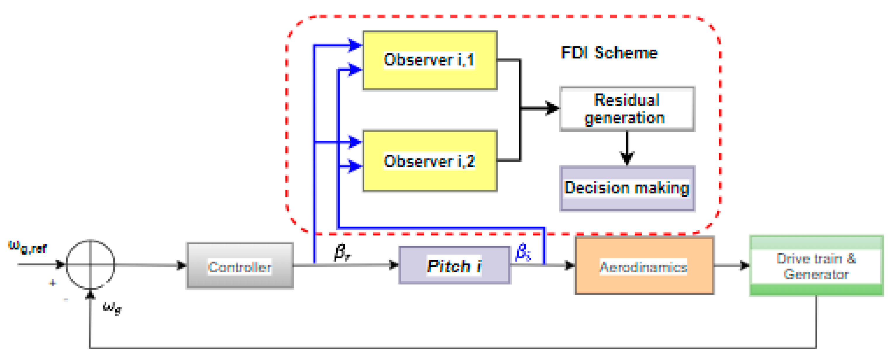
2.3.1. FDI Architecture for Pitch System

In this section, the FDI scheme for each pitch position system is presented. It considers only sensor faults, which are characterized by either a fixed value or a change gain factor on the sensor measurements. Since all three pitch positions are measured with two sensors, the aim of the FDI scheme is to detect and isolate faults in one of the two sensors. In order to perform the detection and isolation of faults in the pitch system, the architecture shown in Figure 3 is proposed. The figure shows the particular configuration of the observer bank used to estimate the pitch angle measurements, which is measured with two sensors for reasons due to hardware redundancy. Since the pitch system is integrated by three identical subsystems, there are a total of six sensors. The configuration of the observer bank allows the observer in charge of estimating the output 1 of pitch i, i.e., observer i , 1 , to use only the measurement of sensor 1 of pitch i. In this way, the observer is sensitive only to faults in that sensor. The residual generator block generates a set of structured residues from the difference between the variables measured and those estimated by the observers. In the decision block, an alarm is generated if any of the residuals exceeds a pre-established threshold, which is established from the behavior of the residuals before and after the fault.
The FDI design only considers that one fault occurs at a time and, therefore, two fault scenarios for each pitch position are considered. The first assumes that sensor 1 is faulty and sensor 2 is healthy. The second assumes sensor 2 is faulty and sensor 2 is healthy. Under this consideration, two residual signals are needed for each pitch position system. Because residual signals are generated from the difference between the estimates of the measurement and real measurement, a set of two sliding mode observers for each pitch position system is needed.
Since sensor faults directly influence the pitch system through the feedback, in order to consider this influence, the function ξ p b i is used to model the position error introduced by the sensor fault. Then, the continuous-time state space model of ith pitch position is as follows:
x ˙ p b i ( t ) = A p b i x p b i ( t ) + B p b i β r e f i ( t ) + D ξ p b i y p b i ( t ) = C p b i x p i ( t )
where x p b i ( t ) = [ β ˙ i ( t ) ,   β i   ] ] T . A p b , B p b and C p b are the system matrices and ξ p b i represents the position error introduced by the sensor fault given by ξ p b i = β i 0.5 i ( β i , m 1 + β i , m 2 ) with i = 1 ,   2 ,   3 .
For system (14), we used the sliding mode observer described in Section 2.2. From Equation (12), two sliding mode observers for the ith pitch position can be designed as:
x ^ ˙ p b 1 i ( t ) = A p b i x ^ p b 1 i ( t ) + B p b i β r e f i ( t ) G l i e y 1 i + G n l i w 1 i y ^ p b 1 i ( t ) = β ^ i , m 1   ( t )
x ^ ˙ p b 2 i ( t ) = A p b i x ^ p b 2 i ( t ) + B p b i β r e f i ( t ) G l i e y 2 i + G n l i w 2 i y ^ p b 2 i ( t ) = β ^ i , m 2   ( t )
where x ^ p b i ( t ) and y ^ p b i denote, respectively, the estimate of state and the estimate of output. G l i and G n l i are appropriate gain matrices to guarantee the stability and convergence of the dynamics of error. The estimation error is defined as e y 1 i = β ^ i , m 1 ( t ) β i , m 1 ( t ) and e y 2 i = β ^ i , m 2 ( t ) β i , m 2 ( t ) . The w represents a discontinuous switched component to induce a sliding motion.
The observer proposed has the capacity to handle the influences of a fault if ξ < σ , where σ represents the gain in the discontinues injection term w and is obtained from Equation (12).
Under this consideration, the sliding mode observer proposed can estimate the state accurately, even in the presence of sensor faults; therefore, it is clear that the estimated ith pitch position must be close to the real value before the fault occurrence and after the sensor fault. To isolate sensor faults, a structured set of residual signals is constructed to be sensitive to only one fault and is given in Table 1.
The residual signal r i , j is used to indicate a fault in the sensor j of the ith-pitch position system, with i = 1 ,   2 ,   3 and j = 1 , 2 . Each residual is sensitive to only one fault. The details of the residual combinations, which are used to isolate different faults, are given by the fault signature.
The following subsection describes the proposed architecture for the transmission train fault diagnosis scheme. In a similar way to the scheme proposed for the pitch system, for the generation of residual signals, an observer bank configuration is proposed.

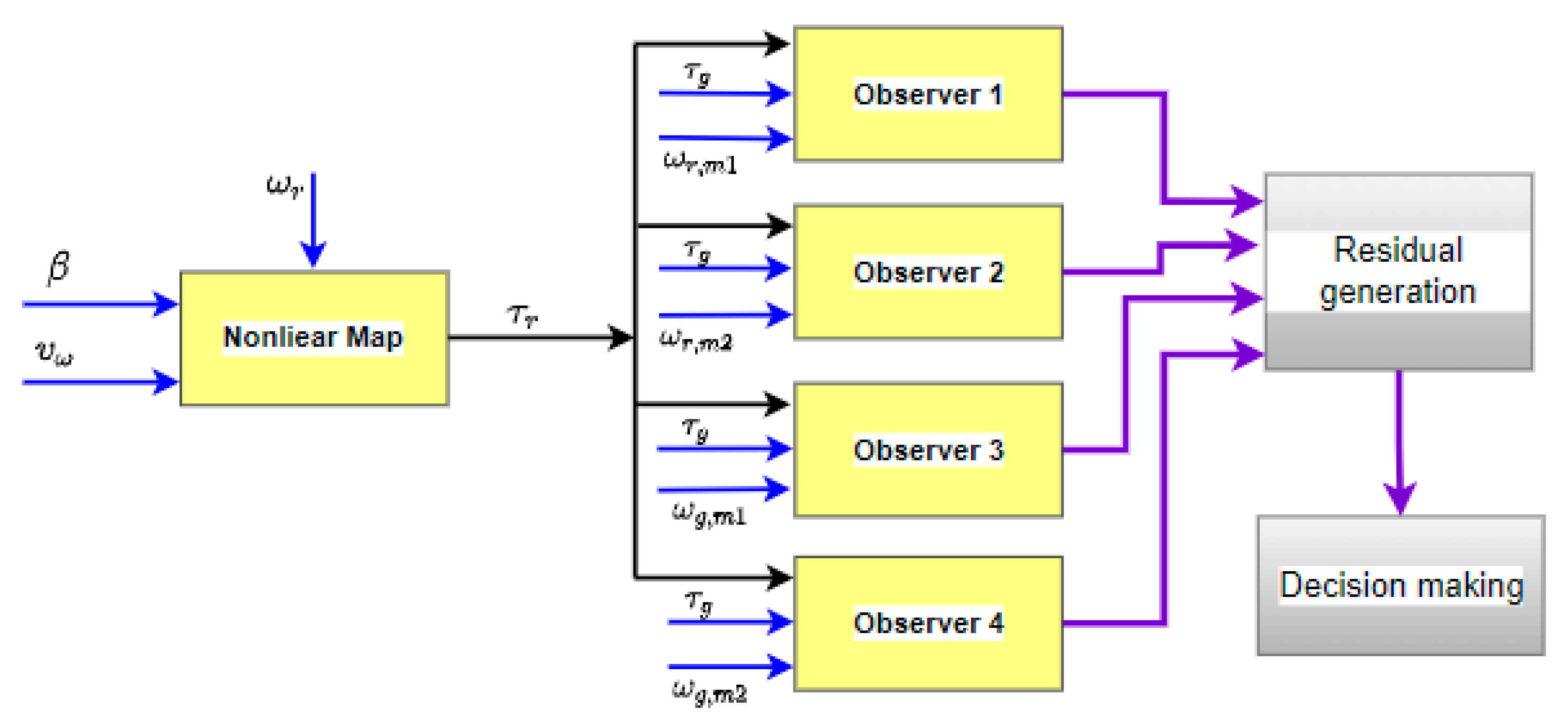
2.3.2. FDI Configurations for Drive Train System

To achieve fault detection and isolation in the drive train, the architecture shown in Figure 4 is proposed, where each observer has all drive train inputs, i.e., rotor torque and generator torque, and only the corresponding sensor measurement. The drive train has hardware redundancy so that the rotor and generator speed measurement is performed with two sensors respectively. Therefore, a bank of four observers is required so that each observer is sensitive only to faults present in the sensor feeding the output signal corresponding to the observer. Since the rotor torque cannot be measured, an estimator based on an algebraic map that depends on the measurement of wind speed, pitch angle, and generator speed is used in this scheme. This algebraic map is described in more detail in [19]. In the residual generator block, the estimation errors of each of the outputs are used as residuals. Then in the decision-making block, an alarm is generated if any of the residuals exceed a preset threshold.
To ensure physical redundancy, both the generator and rotor speed are measured with two sensors. Therefore, the aim of the FDI scheme is to detect and isolate faults in one of the four sensors. Since both the rotor and generator speed are measured using encoders, the fault signals are characterized by either a fixed value or a change gain factor on the sensor measurements. The FDI design only considers that one fault occurs at a time and, therefore, two fault scenarios for both rotor and generator speed sensors are considered. The first assumes that sensor 2 is faulty and sensor 1 is healthy. The second assumes that sensor 1 is faulty and that sensor 2 is healthy. Under this consideration, four residual signals are needed to isolate a fault in the drive train system. Therefore, a set of four sliding mode observers to estimate each sensor measurement was designed.
On the other hand, since the aerodynamic torque is not possible to measure, it depends on wind speed, which can only be roughly measured, and imposes a challenge to the design of the FDI scheme. To overcome this issue, the nonlinear aerodynamics torque is obtained using an aerodynamic torque estimator based on the measured rotor speed ω r , pitch position β i , wind speed v ω , and a mapping of the toque coefficient S (λ, β). It is important to note that due to the difficulty to accurately estimate the aerodynamics torque, an unknown bounded disturbance, ξ d t , is added in the model. The disturbance is modeled as a bounded matching uncertainty entering the system through the input channel.
For the design of the sliding mode observers, consider the model in state space of the drive train system written as
x ˙ d t ( t ) = A d t x d t ( t ) + B d t u d t ( t ) + D ξ d t   y d t ( t ) = C d t x d t ( t )
where x d t ( t ) = [ ω r ( t ) ,   ω g ( t ) , θ Δ ( t ) ] T , u = [ τ r ( t ) τ g ( t ) ] T and A d t , B d t , and C d t are the system matrices, and ξ d t , represents represent the system uncertainty, which are unknown but bounded.
Based on Equation (12), two sliding mode observers of FDI on the drive train are designed, in which ω r ( t ) and ω g ( t ) measurements are used separately.
The proposed sliding mode observers to estimate the rotor speed are given by:
x ^ ˙ d t j ( t ) = A d t ( t ) x ^ d t j ( t ) + B d t u d t ( t ) G l j e y r j + G nl j w r j   y ^ d t r j ( t ) = ω ^ r , m j  
and the proposed sliding mode observers to estimate the generator speed are given by:
x ^ ˙ d t j ( t ) = A d t ( t ) x ^ d t j ( t ) + B d t u d t ( t ) G l j e y g j + G n j v g j   y ^ d t g j ( t ) = ω ^ g , m j  
with e y r j ( t ) = ω ^ r , m j ω r , m j ,   e y g j ( t ) = ω ^ g , m j ω g , m j , and j = 1 , 2 . where ω ^ r , m j and ω ^ g , m j are the rotor speed and generator speed estimations and are computed by observer 1 and 2, respectively. G l and G n l are the observer gains matrices.
The residuals of the FDI scheme are presented in Table 2. From Table 2, each residual is sensitive to only one fault. The residuals r 4 , 1 and r 4 , 2 indicate the rotor speed sensor faults, while the residuals r 5 , 1 and r 5 , 2 indicate the generator speed sensor faults.
In the next section, the effectiveness of the proposed configuration to diagnose faults in both the pitch system and the transmission train is put to the test.

3. Results

In this section, the proposed FDI scheme based on sliding mode observers is tested on the benchmark model of the wind turbine.
The test only considers sensor faults in the pitch system and the drive train. The type of fault is either electrical or mechanical and may result in a fixed value or a change gain factor on the measurements. In general, the severity of these faults is low, but if these are not handled correctly, can result in a breakdown. In order to prevent this situation, early fault detection and isolation are needed.
The wind turbine is a nonlinear system, driven by a disturbance, namely the wind. The residual signals can be nonzero, even when there are no faults. Therefore, the design of the FDI scheme is expected to be robust, in order to achieve a low false alarm rate and a high fault detection rate.
To solve this challenge, the proposed FDI scheme is based on a set of sliding mode observers, robust against disturbances and model uncertainties. The effectiveness of the proposed scheme is demonstrated by a test that includes five sensor faults, three for the pitch and two for the drive train system. These faults are defined in [25] and set as:
First fault: this fault is present at the first pitch system in sensor 1 and outcome in a fixed value:   β 1 , m 1 = 5 ° at time 2000–2100 s.
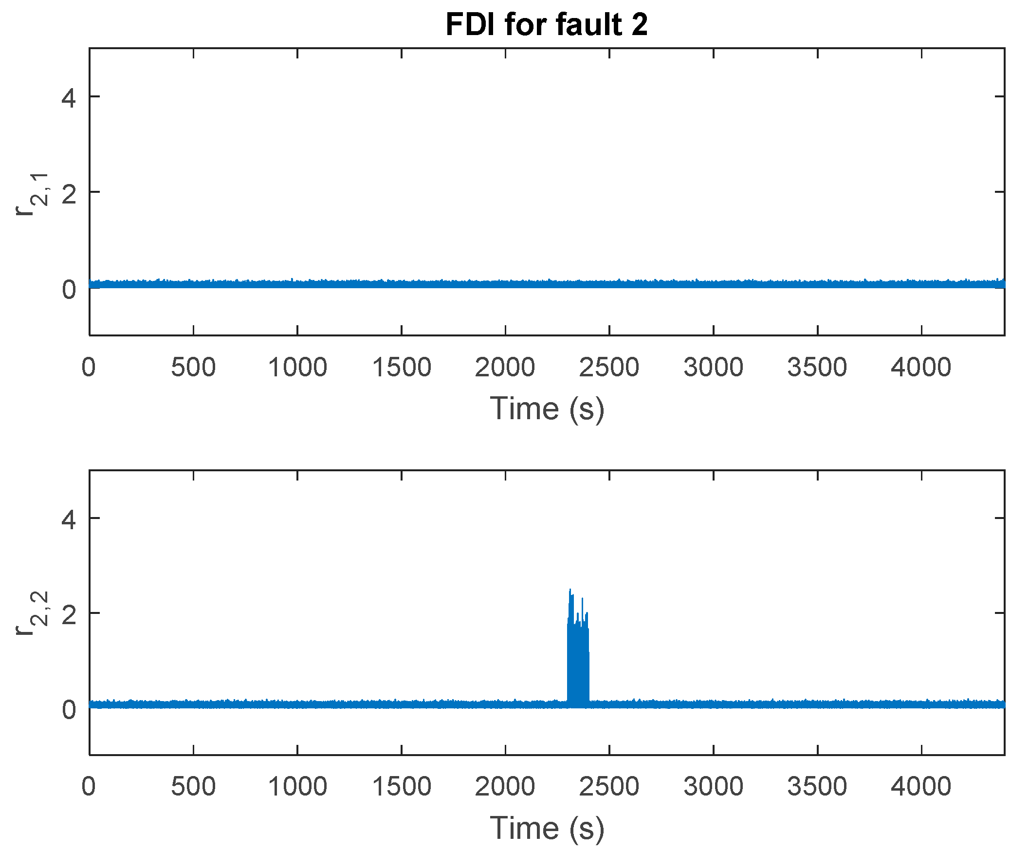
Second fault: the sensor 2 in second pitch system is faulty and outcomes in a gain factor on the measurements: β 2 , m 2 = 1.2 β 2 , m 2 at time 2300–2400 s.
Third fault: the sensor 1 in third pitch system is faulty and outcomes in a fixed value: β 3 , m 1 = 10 ° at time 2600–2700 s.
Fourth fault: the rotor speed sensor signal is faulty and outcomes in a fixed value:   ω r , m 1 = 1.4   rad / s at time 1500–1600 s.
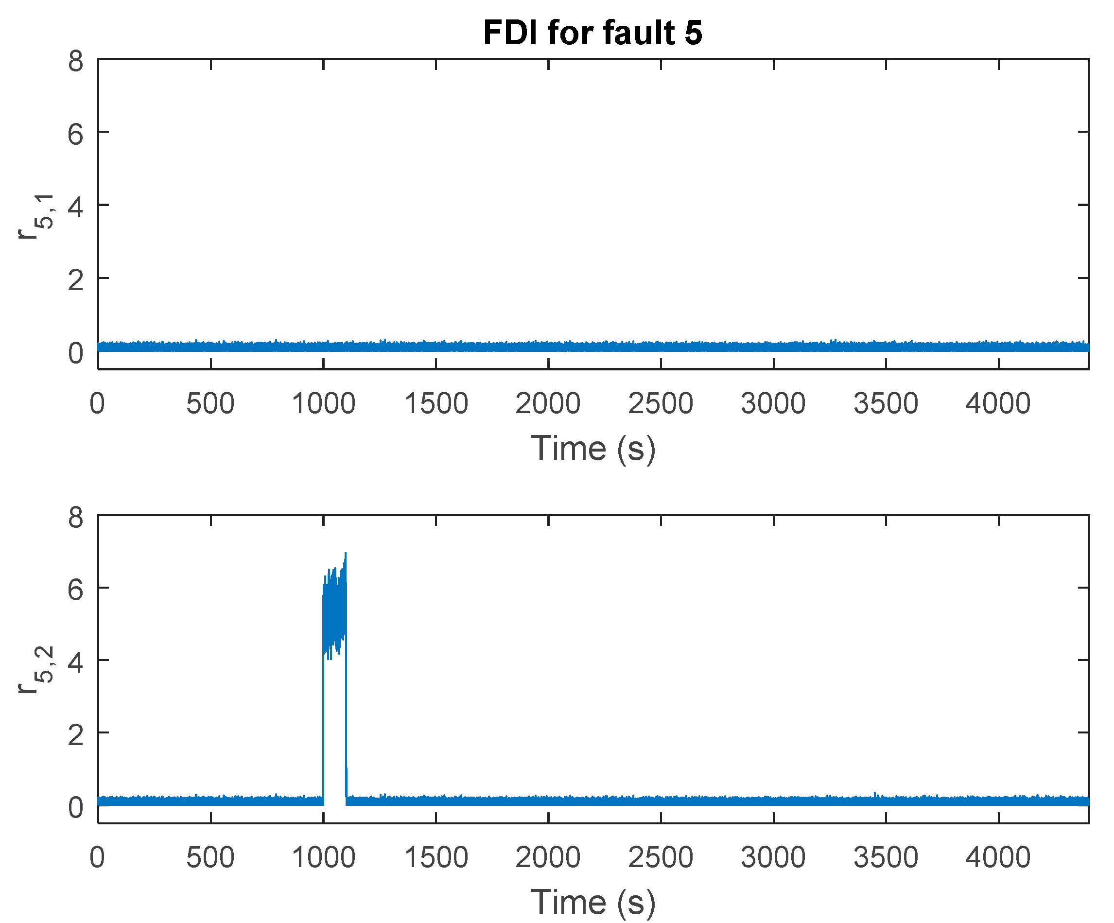
Fifth fault: the generator speed sensor signal is faulty and outcomes in a gain factor on the measurements:   ω g , m 2 = 0.9   ω g , m 2 at time 1000–1100 s.
The results of the FDI scheme for the pitch 1 system when the fault occurs are shown in Figure 5. Fault 1 occurs in sensor 1 of pitch 1, in the time interval from 2000 to 2100 s. As can be seen in the residuals plot in Figure 5, the behavior of the residuals allows identifying the presence of fault 1. It can be observed that the residual r 1 , 1 presents a remarkable abrupt change during the time interval of the occurrence of fault 1, while the residual r 1 , 2 remains very close to zero. Therefore, it can be concluded that a fault occurred in the pitch 1 system, specifically in sensor 1. Ideally, it would be expected that the residuals remain at zero, while there is no fault in the sensors; however, due to the presence of noise in the sensors, the residuals present small deviations around zero, even when the fault has not occurred.
For the pitch 2 system, a scaling fault is considered during a time interval of 2300–2400 s, acting on sensor 2. Figure 6 shows the behavior of the residuals generated from the observer bank in sliding modes. In the graph, it can be noticed that the residual r 2 , 2 presents an erratic behavior in the fault incidence interval, while the residual r 2 , 1 does not present any atypical behavior and remains at a value close to zero. Therefore, from the fault signature of the two residuals, it is shown that the fault occurred in sensor 2 of pitch 2. We should note that the magnitude of the change of the fault-sensitive residual 2 is much smaller with respect to the behavior of the fault-sensitive residual 1. This is because a scaling error fault does not have as noticeable an effect on the sensor signal as a fixed value fault does.
For the pitch 3 system, the fault occurs in sensor 1. It is a fixed value fault acting in the time interval 2600–2700 s. The results of the fault detection scheme in the pitch 3 system are presented in Figure 7. It can be observed that fault 3 can be detected by means of the residual r 3 , 1 , which presents a significant deviation in the time interval of the fault. While the residual r 3 , 2 does not present significant changes, it remains very close to zero. From the behavior of the residuals of the pitch system, it can be observed that these were shown to be sensitive to the presence of faults, thus solving the problem of fault detection in the pitch system. Moreover, since each of the presented residuals was shown to be sensitive to only one fault, fault isolation is achieved with the help of the fault signature table.
The proposed scheme for the detection and isolation of faults in the drive train employs a bank of four observers whose function is to estimate the turbine rotor speed and the generator speed. From the difference between the estimates made by the observers and the measurements obtained by the sensors, a set of four residuals is generated. Figure 8 shows the behavior of the residuals designed to be sensitive to fault 4. Fault 4 corresponds to a scaling error in the signal of sensor 1 in charge of measuring the rotor speed. Since sensor 2 is fault free, it can be observed that the residual r 4 , 2 remains practically invariant during the whole simulation interval. While the residual r 4 , 1 shows an atypical behavior during the1500–1600 s interval. The magnitude of the deviation observed in the residual in the mentioned interval is high enough to infer the presence of a fault in the sensor.
Finally, the behavior of the residuals sensitive to fault 5 is shown in Figure 9. Fault 5 is a fixed value in sensor 2 responsible for measuring the generator speed, during the time interval 1000–1100 s. It is important to note that, from the point of view of fault dynamics, in a fixed value fault a more significant deviation of the residual can be observed, this compared to the case of a scaling error type fault. This is evident in the magnitude of the deviation of the residual r 5 , 2 . From which it can be concluded that a fault has occurred in sensor 2 responsible for the measurement generator speed. While the behavior of the residual r 5 , 1 confirms that sensor 1 is free of fault.

4. Discussion

The faults considered in this paper only cover the pitch system and drive train, and since these are modeled independent, an FDI scheme was designed separately for each one. The FDI scheme proposed for the pitch system considers the error introduced by sensor faults as an uncertainty acting on the input channel. Under this condition, a sliding mode observer bank was capable of estimating the system outputs, even in the presence of faults is proposed. The differences between the estimates made by the observers and the sensor measurements were used to regenerate a structured set of residuals for each pitch system. The structure of the FDI scheme for the pitch system is shown in Figure 3. It considers a set of six observers. To detect sensor faults, each sliding mode observer is dedicated to detect one sensor fault and generate one residual. The residual signals are generated from the measurements and estimates made by the bank of observers. After successful fault detection, the next task is to isolate the faults, which is done using a signature Table 1.
Secondly, to overcome the problem of coupled dynamics and the absence of aerodynamic torque measurement, the proposed FDI approach for the drive train employed an aerodynamic torque estimator based on an algebraic map. The uncertainty associated with the estimation was modeled as a disturbance in the input channel of the system model. The aerodynamic torque estimate was fed to a bank of observers in sliding modes each of which employed different sensor measurements in order to be sensitive to only one fault. Each observer was dedicated to one sensor fault; consequently, the generated residual was sensitive to only one sensor fault. For the task of isolating the faults, a signature Table 2 was used.
The effectiveness of the FDI schemes is demonstrated from the evaluation of five sensor fault scenarios as described in the results section. Due to the measurement noises and the uncertainties in the system, the residual signals are not zero, even for the fault-free case. To overcome this issue, residual evaluation and threshold are employed. The thresholds are designed based on the expressions of the residuals and uncertainties and measurement noise in the system. From the results presented in the last section, it can be easily seen that the residual remains around zero before and after the occurrence of fault, but during the fault interval, the residual rises significantly. To achieve a low false alarm, the thresholds are set at the maximum absolute value of the residuals. Therefore, a fault is presented in the system if it causes significant deviations from zero on some of the residuals.

5. Conclusions

In this article, a fault detection and isolation approach is proposed for the sensors of the pitch system and drive train in a benchmark wind turbine model. This approach employs a bank of sliding mode observers, designed to receive all of the inputs of the system and only one measurement of the set of available sensors. This allows each observer to be sensitive only to faults present in the sensor input signal. The dynamics introduced by the fault in a sensor of the pitch system, as well as the uncertainty associated with the estimation of the rotor torque in the transmission train, are modeled as disturbances acting on the input channel of their respective subsystem. Under this condition, the convergence of the observers turns out to be independent of the fault dynamics and the uncertainty present in the system. The difference between observer bank outputs and the measurements of the sensors is used to generate a structured set of residues for the pitch system and the drive train. It is shown that the residuals are capable of detecting a sensor fault occurrence, and, on the other hand, they remain very close to zero when the system is fault-free. This allows decision-making on fault detection using the concept of a fixed threshold. The value of the thresholds was selected based on the behavior of the residues before and after the appearance of the fault. To achieve fault isolation, fault signature matrix constructed from the residuals was used.

Author Contributions

Conceptualization, V.B.-J. and M.A.-M.; methodology, V.B.-J. and B.Y.L.-Z.; software, V.B.-J. and E.M.S.C.; validation, V.B.-J. and M.A.-M.; formal analysis, M.A.-M. and V.B.-J.; investigation, V.B.-J., M.A.-M. and B.Y.L.-Z.; resources, M.A.-M., B.Y.L.-Z., E.M.S.C., L.C.P.; writing—original draft preparation, V.B.-J., B.Y.L.-Z., L.G.V.V.; writing—review and editing, M.A.-M., E.M.S.C., V.B.-J., L.G.V.V., L.C.P.; supervision, M.A.-M. All authors have read and agreed to the published version of the manuscript.

Funding

This research received no external funding.

Institutional Review Board Statement

Not applicable.

Informed Consent Statement

Not applicable.

Data Availability Statement

Not applicable.

Acknowledgments

The development of this project is the product of the support provided by the National Council of Science and Technology (CONACYT), the National Technological Institute of Mexico (TecNM)/CENIDET.

Conflicts of Interest

The authors declare no conflict of interest.

Nomenclature

A System matrix
B Input matrix
C Output matrix
D Distribution matrix
e Estimation error
F Viscous friction
G Observer gain
H Torsion damping coefficient
J Moment of inertia
K Torsion stiffness
N Gear ratio
P Power
R Rotor ratio
r Residual signal
S Power coefficient
T Change of Coordinates Matrix
v Wind speed
w Discontinue function
x System states
x ^ Estimate of x
y Output system
y ^ Estimate of y
α a known function
β Pitch angle
γ Cutoff frequency
ζ Damping coefficient
η Efficiency
θ Torsion angle
λ Tip speed ratio
ξ Bounded uncertainty
ρ Wind density
σ Scalar
τ Torque
ψ Natural frequency
ω Speed
Subscripts
d t Drive train
g Generator
l Linear
n l Nonlinear
p b Pitch blade
r Rotor
r e f Reference
ω Wind

References

  1. Sawant, M.; Thakare, S.; Rao, A.; Feijóo-Lorenzo, A.; Bokde, N. A Review on State-of-the-Art Reviews in Wind-Turbine- and Wind-Farm-Related Topics. Energies 2021, 14, 2041. [Google Scholar] [CrossRef]
  2. Mazzeo, D.; Matera, N.; De Luca, P.; Baglivo, C.; Congedo, P.M.; Oliveti, G. A literature review and statistical analysis of photovoltaic-wind hybrid renewable system research by considering the most relevant 550 articles: An upgradable matrix literature database. J. Clean. Prod. 2021, 295, 126070. [Google Scholar] [CrossRef]
  3. Pfaffel, S.; Faulstich, S.; Rohrig, K. Performance and Reliability of Wind Turbines: A Review. Energies 2017, 10, 1904. [Google Scholar] [CrossRef] [Green Version]
  4. Márquez, F.P.G.; Tobias, A.M.; Pérez, J.M.P.; Papaelias, M. Condition monitoring of wind turbines: Techniques and methods. Renew. Energy 2012, 46, 169–178. [Google Scholar] [CrossRef]
  5. Bianchi, F.D.; De Battista, H.; Mantz, R.J. Wind Turbine Control Systems: Principles, Modelling and Gain Scheduling Design; Springer: London, UK, 2007; Volume 19. [Google Scholar]
  6. Alaskari, M.; Abdullah, O.; Majeed, M.H. Analysis of Wind Turbine Using QBlade Software. IOP Conf. Series Mater. Sci. Eng. 2019, 518, 032020. [Google Scholar] [CrossRef]
  7. Raut, S. Simulation of Micro Wind Turbine Blade in Q-Blade. Int. J. Res. Appl. Sci. Eng. Technol. 2017, 5, 256–262. [Google Scholar] [CrossRef]
  8. Chaudhary, M.; Roy, A. Design & optimization of a small wind turbine blade for operation at low wind speed. World J. Eng. 2015, 12, 83–94. [Google Scholar] [CrossRef]
  9. Liu, J.; Yao, Q.; Hu, Y. Model predictive control for load frequency of hybrid power system with wind power and thermal power. Energy 2019, 172, 555–565. [Google Scholar] [CrossRef]
  10. Chen, J.; Patton, R.J. Robust Model-Based Fault Diagnosis for Dynamic Systems; Springer Science & Business Media: Berlin/Heidelberg, Germany, 1999; Volume 11. [Google Scholar]
  11. Luo, G.; Hurwitz, J.; Habetler, T.G. A survey of multi-sensor systems for online fault detection of electric machines. In Proceedings of the 2019 IEEE 12th International Symposium on Diagnostics for Electrical Machines, Power Electronics and Drives (SDEMPED), Toulouse, France, 27–30 August 2019; pp. 338–343. [Google Scholar]
  12. Janssens, O.; Loccufier, M.; Van Hoecke, S. Thermal Imaging and Vibration-Based Multisensor Fault Detection for Rotating Machinery. IEEE Trans. Ind. Inform. 2019, 15, 434–444. [Google Scholar] [CrossRef] [Green Version]
  13. Luwei, K.C.; Yunusa-Kaltungo, A.; Sha’Aban, Y.A. Integrated fault detection framework for classifying rotating machine faults using frequency domain data fusion and Artificial Neural Networks. Machines 2018, 6, 59. [Google Scholar] [CrossRef] [Green Version]
  14. Yunusa-Kaltungo, A.; Cao, R. Towards Developing an Automated Faults Characterisation Framework for Rotating Machines. Part 1: Rotor-Related Faults. Energies 2020, 13, 1394. [Google Scholar] [CrossRef] [Green Version]
  15. Cao, R.; Yunusa-Kaltungo, A. An Automated Data Fusion-Based Gear Faults Classification Framework in Rotating Machines. Sensors 2021, 21, 2957. [Google Scholar] [CrossRef] [PubMed]
  16. Chen, W.; Ding, S.; Haghani, A.; Naik, A.; Khan, A.; Yin, S. Observer-based FDI Schemes for Wind Turbine Benchmark. IFAC Proc. Vol. 2011, 44, 7073–7078. [Google Scholar] [CrossRef]
  17. Hwas, A.; Katebi, R. Model-based fault detection and isolation for wind turbine. In Proceedings of the 2012 UKACC International Conference on Control, Cardiff, UK, 3–5 September 2012; pp. 876–881. [Google Scholar]
  18. XiaHou, K.; Li, M.S.; Liu, Y.; Wu, Q.H. Sensor Fault Tolerance Enhancement of DFIG-WTs via Perturbation Observer-Based DPC and Two-Stage Kalman Filters. IEEE Trans. Energy Convers. 2017, 33, 483–495. [Google Scholar] [CrossRef]
  19. Sharan, B.; Jain, T. Actuator and Sensor Fault Diagnosis for Wind Energy Conversion Systems. In Proceedings of the 2018 15th International Conference on Control, Automation, Robotics and Vision (ICARCV), Singapore, 18–21 November 2018; pp. 955–959. [Google Scholar]
  20. Zhang, X.; Zhang, Q.; Zhao, S.; Ferrari, R.; Polycarpou, M.; Parisini, T. Fault detection and isolation of the wind turbine benchmark: An estimation-based approach. IFAC Proc. Vol. 2011, 44, 8295–8300. [Google Scholar] [CrossRef] [Green Version]
  21. Odgaard, P.F.; Stoustrup, J. Unknown input observer based detection of sensor faults in a wind turbine. In Proceedings of the 2010 IEEE International Conference on Control Applications, Yokohama, Japan, 8–10 September 2010; pp. 310–315. [Google Scholar]
  22. Mokhtari, A.; Belkheiri, M. An adapative observer based FDI for wind turbine benchmark model. In Proceedings of the 2016 8th International Conference on Modelling, Identification and Control (ICMIC), Algiers, Algeria, 15–17 November 2016; pp. 742–746. [Google Scholar]
  23. Dey, S.; Pisu, P.; Ayalew, B. A Comparative Study of Three Fault Diagnosis Schemes for Wind Turbines. IEEE Trans. Control Syst. Technol. 2015, 23, 1853–1868. [Google Scholar] [CrossRef]
  24. Ziyabari, S.H.S.; Shoorehdeli, M.A.; Karimirad, M. Robust fault estimation of a blade pitch and drivetrain system in wind turbine model. J. Vib. Control 2021, 27, 277–294. [Google Scholar] [CrossRef]
  25. Song, D.; Yang, J.; Dong, M.; Joo, Y.H. Kalman filter-based wind speed estimation for wind turbine control. Int. J. Control Autom. Syst. 2017, 15, 1089–1096. [Google Scholar] [CrossRef]
  26. Edwards, C.; Spurgeon, S. Sliding Mode Control: Theory and Applications; CRC Press: Boca Raton, FL, USA, 1998. [Google Scholar]
  27. Habibi, H.; Howard, I.; Simani, S.; Fekih, A. Decoupling Adaptive Sliding Mode Observer Design for Wind Turbines Subject to Simultaneous Faults in Sensors and Actuators. IEEE/CAA J. Autom. Sin. 2021, 8, 837–847. [Google Scholar] [CrossRef]
  28. Odgaard, P.F.; Stoustrup, J.; Kinnaert, M. Fault-tolerant control of wind turbines: A benchmark model. IEEE Trans. Control Syst. Technol. 2013, 21, 1168–1182. [Google Scholar] [CrossRef] [Green Version]
  29. Edwards, C.; Spurgeon, S. On the development of discontinuous observers. Int. J. Control 1994, 59, 1211–1229. [Google Scholar] [CrossRef]
  30. Edwards, C.; Spurgeon, S.; Patton, R.J. Sliding mode observers for fault detection and isolation. Automatic 2000, 36, 541–553. [Google Scholar] [CrossRef]
  31. Simani, S.; Fantuzzi, C.; Patton, R.J. Model-Based Fault Diagnosis Techniques. In Advances in Industrial Control; Springer: London, UK, 2003; pp. 19–60. [Google Scholar]
Figure 1. Interconnection of subsystems of the wind turbine in benchmark.
Processes 10 00054 g001
Figure 2. Architecture of observer-based FDI.
Processes 10 00054 g002
Figure 3. Architecture for FDI in the pitch system.
Processes 10 00054 g003
Figure 4. FDI architecture for drive train.
Processes 10 00054 g004
Figure 5. Faults in the first pitch system.
Processes 10 00054 g005
Figure 6. Fault bias in the second pitch during the time 2300 to 2400 s.
Processes 10 00054 g006
Figure 7. Fault bias in the third pitch during the time 2600 to 2700 s.
Processes 10 00054 g007
Figure 8. The abrupt fault of rotor speed sensor 1 in the time period of 1500 to 1600 s.
Processes 10 00054 g008
Figure 9. The abrupt fault in the speed of the generator in the period time of 1000 to 1100 s.
Processes 10 00054 g009
Table 1. Pitch system FDI logic.
ResidualsDefinitionFault 1Fault 2Fault3
r 1 , 1 β ^ 1 , m 1 β 1 , m 1 100
r 1 , 2 β ^ 1 , m 2 β 1 , m 2 000
r 2 , 1 β ^ 2 , m 1 β 2 , m 1 000
r 2 , 2 β ^ 2 , m 2 β 2 , m 2 010
r 3 , 1 β ^ 3 , m 1 β 3 , m 1 000
r 3 , 2 β ^ 3 , m 2 β 3 , m 2 001
Table 2. Drive train system FDI logic.
ResidualsDefinitionFault 4Fault 5
r 4 , 1 y ^ d t r 1 ω r , m 1 10
r 4 , 2 y ^ d t r 2 ω r , m 2 00
r 5 , 1 y ^ d t g 1 ω g , m 1 00
r 5 , 2 y ^ d t g 2 ω g , m 2 01
Publisher’s Note: MDPI stays neutral with regard to jurisdictional claims in published maps and institutional affiliations.

