
Multi-Objective Optimization for the Radial Bending and Twisting Law of Axial Fan Blades
by
 , ,
, ,
Yanyan Ding
1, 
Jun Wang
1,*,
Boyan Jiang
1,
Zhiang Li
1,
Qianhao Xiao
1, 
Lanyong Wu
2 and
Bochao Xie
2 1
School of Energy and Power Engineering, Huazhong University of Science and Technology, Luoyu Road No.1037, Wuhan 430074, China
2
Guang Dong Nedfon Air System Co., Ltd., Taicheng Road No.15, Taishan 529200, China
*
Author to whom correspondence should be addressed.
Processes 2022, 10(4), 753; https://0-doi-org.brum.beds.ac.uk/10.3390/pr10040753
Submission received: 13 March 2022
/
Revised: 7 April 2022
/
Accepted: 8 April 2022
/
Published: 13 April 2022
Abstract
:The performance of low-pressure axial flow fans is directly affected by the three-dimensional bending and twisting of the blades. A new blade design method is adopted in this work, where the radial distribution of blade angle and blade bending angle is composed of standard-form rational quadratic Bézier curves. Dendrite Net is then trained to predict the pneumatic performance of the fan. A non dominated sorting genetic algorithm is employed to solve the global optimization problem of the total pressure coefficient and efficiency. The simulation results show that the optimal blade load distribution along the radial direction becomes uniform, and the suction surface separation vortex and passage vortex are restrained. On the other hand, the tip leakage vortex is enhanced and moves toward the blade leading edge. According to the experimental results, the maximum efficiency increases by 5.44%, and the maximum total pressure coefficient increases by 2.47% after optimization.
1. Introduction
The axial fan is a core component of the pipeline system and is widely applied in air ventilation and transport devices. As carbon neutralization is becoming increasingly important due to global warming, reducing flow loss and increasing fan efficiency are necessary.
The modern fan design method realizes passive control of the internal flow by changing the three-dimensional structure of the rotor. Li et al. [1] investigated the performance change of axial fans with impeller trimming quantities of 5%, 10%, and 15% of the blade height. Pascu et al. [2] optimized the blade profile by the three-dimensional inverse method to achieve the minimum loss in an axial fan. Ye et al. [3] designed several blade tip patterns to explore the relationship between the shape of the groove tip and leakage losses. Pogorelov et al. [4] proposed two tip clearance ratio widths to research the turbulent transition near the blade suction surface. Further research has focused on performance improvement using skewed and swept blades. Rzadkowski et al. [5,6] analyzed unsteady forces acting on rotor blades of compressors and explored the influencing factor of the low-frequency and high-frequency harmonics. In the process of blade design, the bending and twisting laws of the blade in the radial direction directly affect the radial load distribution of the impeller, thereby affecting the internal flow of the fan. However, few studies have focused on the radial bending and twisting of blades.
Fan performance optimization by numerical simulation requires significant computing resources. With the continuous improvement of deep computational learning, performance prediction by establishing an approximate model of fluid machinery has been extensively applied in fluid machinery design. Ghorbanian and Gholamrezaei et al. [7] compared the prediction accuracy of different types of artificial neural networks (ANNs), obtaining good agreement between the experimental and predictive data using a multilayer perceptron network. Cortés et al. [8] employed ANNs to predict the compressor pressure ratio and isentropic efficiency, while Kamar et al. [9] developed an ANN to predict the cooling capacity of an air-conditioning system. The prediction methods mentioned above are black-box systems, which means that the performance map can be successfully obtained. However, identifying the impact of different input parameters on the fan efficiency and the total pressure is challenging.
In this study, bending and twisting laws constructed by Bézier curves are adopted for the blade design and optimization of a low-pressure axial flow fan. Dendrite Net (DD), a new white-box system, is then introduced to establish the mapping between blade modeling parameters and impeller performance. While predicting the performance of the fan, the relation spectrum is obtained, which reflects the influence of different input parameters on the fan’s performance. The input parameters with the most significant influence on fan performance are selected according to the relationship spectrum, and the corresponding constraint conditions are set. Finally, a multi-objective genetic algorithm is introduced to optimize the fan pressure and efficiency.
2. Research Objective
2.1. Geometric Model
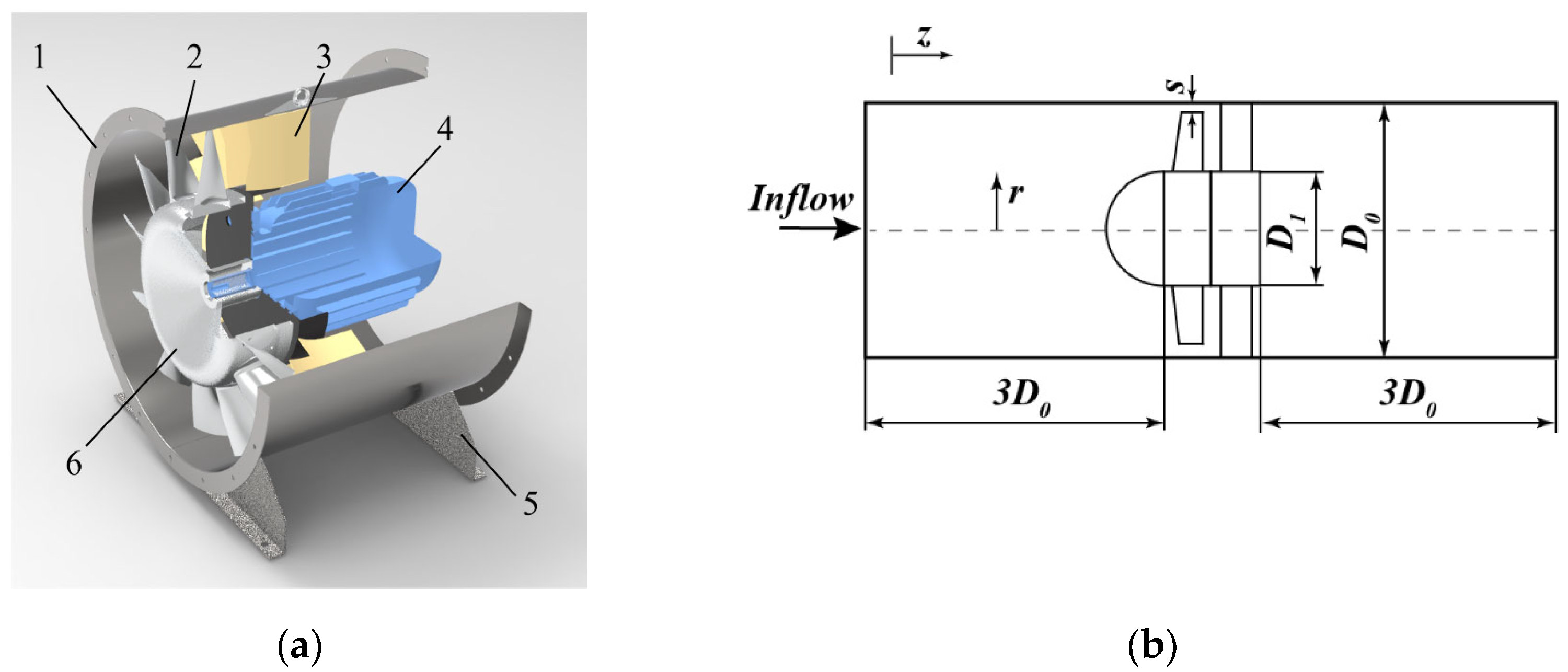
We employ an industrial low-pressure axial fan with a rear guide blade structure as the prototype for multi-objective optimization problems in this study. As shown in Figure 1a, the fan is composed of an impeller, rear guide vane, machine shell, and other flow-passing parts. The axial fan located in the pipeline is shown in Figure 1b and is part of the air conveying system’s air supply component. An extension section is located at the inlet and outlet of the fan system to reproduce the actual flow, and the motor embedded in the fan center exerts specific flow resistance on the fan. The flow field is simplified to facilitate analysis by removing complex structures in the following simulation. Table 1 summarizes the key design parameters of the original axial fan.
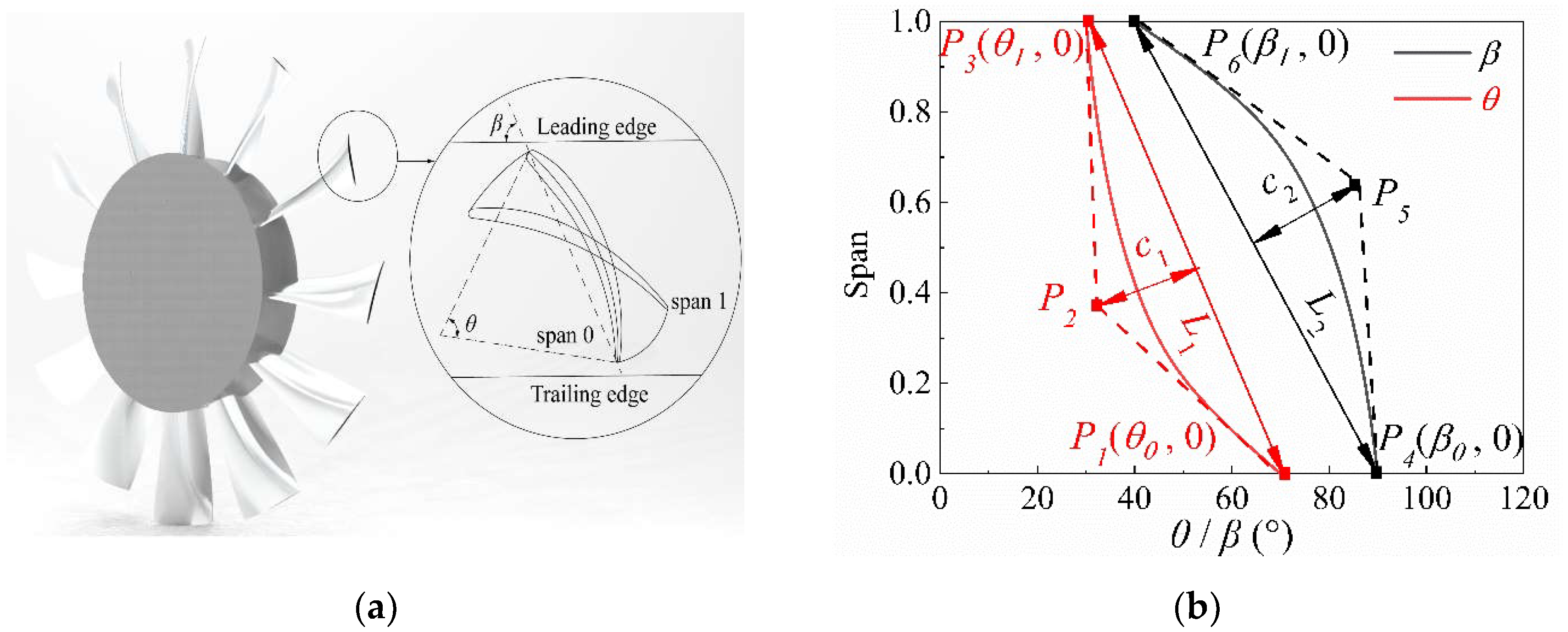
A new blade design method is adopted in this study. The mean camber line is a circular curve. The blade pattern is generated by a NACA 65-010 airfoil developed by the National Advisory Committee for Aeronautics (NACA) [10]. Here, we define the angle between the chord and leading-edge as the blade angle β and define the central angle of the mean camber line as the blade bending angle θ. The angle position is shown in Figure 2a, where “span 0” represents the base of the blade and “span 1” represents the top position of the blade. The distribution of blade angle β along the span determines the blade twist law, and the distribution of blade bending angle θ along the span determines the blade bending law.
The radial distribution of θ and β is composed of standard-form rational quadratic Bézier curves [11,12]. The position of the three control points determines the shape of each curve. Figure 2b shows the radial distribution curves of θ and β along the spanwise direction. The distribution curves are created by the second-order rational Bézier curve, whose shape is determined by three control points. Taking the distribution of θ as an example, the x-coordinate of control points P1 and P3 represent the θ at spans 0 and 1. The camber of the θ distribution curve (A), which is determined by the position of point P2, is defined as follows:
where: c1 is the distance between P2 and ; L1 is the distance between P1 and P3; and “±” is the curve concavity and convexity.
Similarly, the camber of the β distribution curve (B) can be defined as:
where: c2 is the distance between P5 and ; L2 is the distance between P4 and P6; and “±” is the curve concavity and convexity.
2.2. Numerical Method
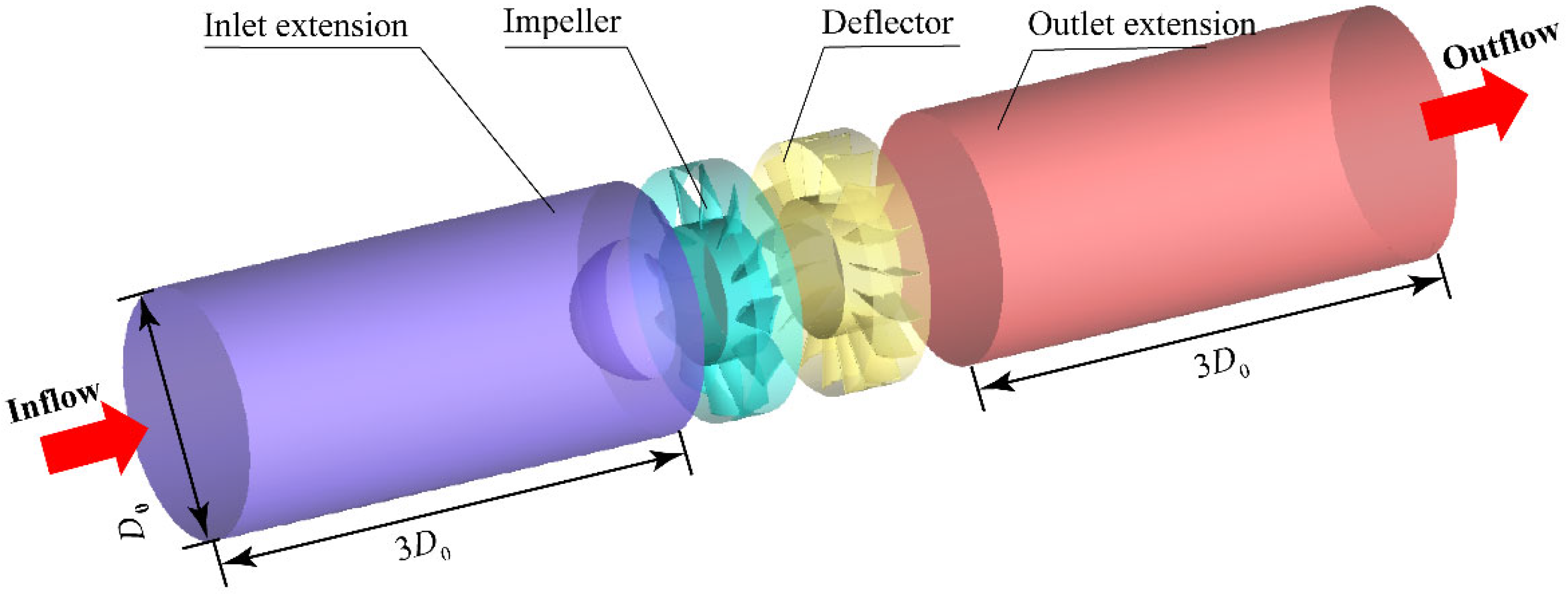
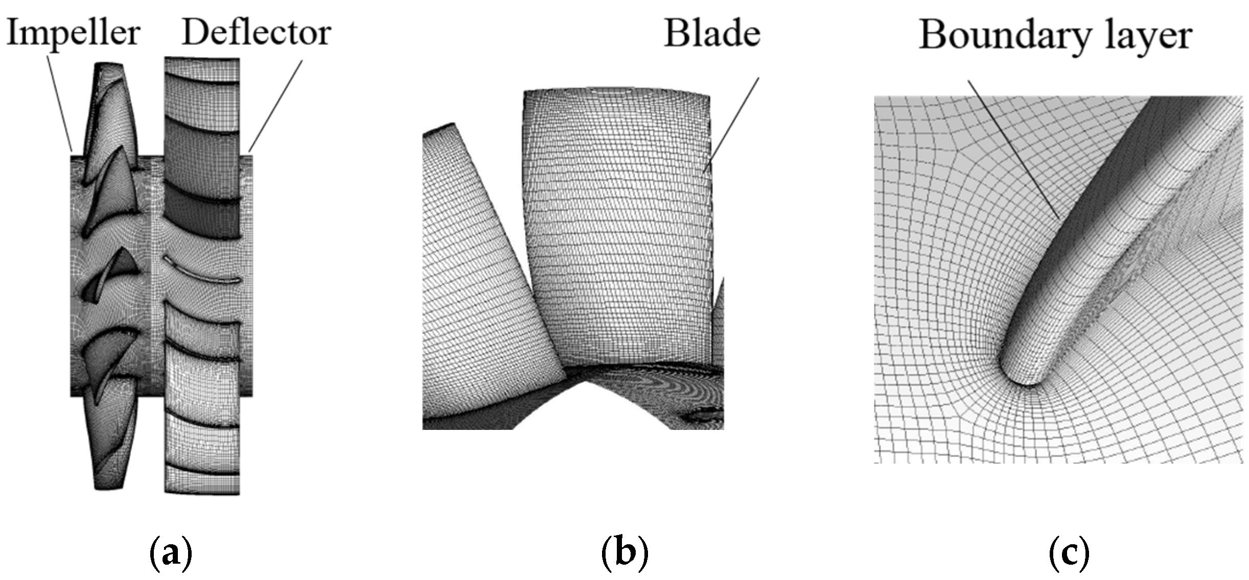
The three-dimensional (3D) numerical simulation of the fan system is carried out using the computational fluid dynamics (CFD) software Fluent to acquire the internal flow of the fans. The computing domain of the fan system is shown in Figure 3, where the whole domain is divided into inlet extension, impeller, deflector, the outlet extension. Both the inlet and outlet extensions are obtained by extending the adjacent interfaces to the length of 3D0 [13]. A fine hexahedral mesh is applied to capture the details in the flow field. The mesh model of the key parts, such as the impeller and deflector, is locally encrypted to ensure the appropriateness of the average y+ near the wall shear. The mesh model is shown in Figure 4.
Three-dimensional steady simulations are performed by solving the incompressible Reynolds-averaged Navier–Stokes (RANS) equations in Fluent’s commercial CFD software. The realizable k–ε [14] is adopted, which was proven to be effective in calculating the turbulent viscosity accurately in previous studies [15].
We set the inlet boundary condition as the velocity-inlet. The inlet air is considered to be fully developed, and the turbulence intensity and turbulence viscosity ratios are set to 5% and 10%, respectively. The outlet boundary condition is set as the outflow. The SIMPLEC algorithm is adopted for the pressure velocity coupling method, and the multiple reference frame (MRF) is used to deal with rotor stator interference. The second-order upwind scheme is imposed as the convection term, and the pressure and diffusion term is the central difference scheme [16].
2.3. Grid Independence
Mesh precision has a significant effect on the accuracy of the fan performance simulation. In this study, various grid models are established to increase the grid quantity from 2.6 million to 11.02 million. After solving the flow field inside the fan, the physical quantities in the calculation domain are counted to calculate the performance parameters of the fan as follows:
where is the outlet section’s average total pressure (or static pressure) of the outlet section, is the average total pressure (or static pressure) of the inlet section, is the volume flow rate of the fan, is the impeller torque, and is the rotation angular velocity of the impeller.
The aerodynamic performance of the original axial fan is investigated in a ducted test device, following the performance testing standard of the International Organization for Standardization (ISO) 5801:2017 Industrial fans—performance testing using standardized airways [17]. Figure 5 shows the structure diagram of the fan test system and a photograph of the fan test site.
The results of grid independence are provided in Figure 6. In this figure, the predicted and change with the grid quantity. The performance curves of the experiment exhibit the same trend as that of the simulation results. When the number of grids is small, the calculated total pressure and efficiency are greater than the experimental values. The calculated performance parameters gradually move closer to the experimental value as the grid density increases. When the grid quantity exceeds 11.0 × 10⁶, the change rate of performance parameters is less than 1%. In this case, we believe that the fan performance does not change with the number of model grids. The grid quantity in each flow area is shown in Table 2.
The deviation in maximum total pressure (εPtF) and maximum efficiency (εη) and are 3.02% and 2.28%, respectively. Based on the authors’ knowledge, the deviation is mainly caused by two factors. The first is the simplifition of geometry, as the motor structure is simplified to generate a series of high-quality full-structured meshes. The second is due to inevitable errors in both the numerical simulation and the experimental test. The deviation between the calculated and experimental data is lower than 5%, which is acceptable according to previous studies [18,19,20,21]. The total grid quantity selected eventually reaches approximately 11.02 × 10⁶.
3. Optimization
3.1. Optimization Objective
The nonlinear second-order consolidation differential Navier–Stokes equation is used to predict the performance of axial flow fans. Thus, the fan optimization mathematical model is a complex nonlinear problem with constraints and multiple peak values. In this study, the optimization variables are six parameters that determine the spanwise distortion laws of the fan. The optimization objectives are maximizations of the total pressure coefficient and maximum efficiency, marked as ψOPT and ηOPT. The flow coefficient is in the range of 0.24–0.45 The mathematical model of the optimization process can be expressed as a search: X = (θ0, θ1, A, β0, β1, B) with the constraint , so that:
where represents the number of constraints, C is the constraint limit value, m is the number of working conditions, n is the number of objective functions, is the linear weighted average of the kth objective function, and represents the weighting factor of the kth objective function under the ith working condition [22].
3.2. Optimization Process
We adopt the Latin hypercube design method (LHD) [23] to generate a sample space of six variables. The impeller design platform is built based on MATLAB, and the impeller model and computing grid are generated in batches. The total pressure coefficient (ψOPT) and efficiency (ηOPT) of the fan are then predicted by CFD numerical simulation, and the original sample database is established. Enormous computing resources are needed to complete the numerical calculation of all samples in genetic algorithm optimization. Dendrite Net (DD) [24] is introduced to improve optimization efficiency to establish a variable mapping between the impeller and performance parameters. The predicted fan performance parameters are obtained by training the DD network. Finally, DD is coupled with the non-dominated sorting genetic algorithm-II (NSGA-II) [25]. The optimization process was finished once the prediction results reach the termination conditions of the genetic algorithm. The optimization process is shown in Figure 7.
3.3. Dendrite Net
Dendrite Net (DD) is an essential machine learning algorithm that is similar to support vector machines (SVMs) or multi-layer perceptron (MLP). It transforms the fan system to a Taylor expansion, through which we can identify the importance of the system parameters. A graphical illustration of the learning process is shown in Figure 8, where X denotes the input space of the DD, Al is the input of the lth DD module and output of the (l-1)th DD module, and W l,l−1 is the weight matrix from the (l-1)th module. Additionally, ◦ is the Hadamard product, L expresses the number of modules, and Y denotes the output space of DD.
The forward-propagation of the DD and liner modules is denoted as:
The error-backpropagation of DD and linear modules is:
The weight adjustment of DD is:
where and Y are the DD’s outputs and labels, respectively, m denotes the number of training samples in one batch, and the learning rate α can either be adapted with epochs or fixed to a small number based on heuristics [26].
Employing the six blade parameters generated by LHD, the maximum total pressure coefficient ψOPT and maximum efficiency ηOPT are obtained by numerical simulation. The initial sample space used to train the DD network is obtained from the LHD method (shown in Table 3).
A total of 40 groups are collected in the initial sample space. In order to predict the ψOPT and ηOPT, the DD is trained twice.
Each column in the sample space is first normalized. The normalized equation is as follows [27]:
where is column i of the normalized sample space, is the column i of the original sample space, is the maximum value in , and is the minimum values in .
The normalized impeller structural parameters are then set as input variables, and the corresponding impeller performance parameters are set as output variables. The effect of each blade parameter on fan performance is a complex nonlinear problem. In order to clearly explore the influence of each parameter on fan performance parameters, two Dendrite Nets with six modules are trained to predict the ψOPT and ηOPT.
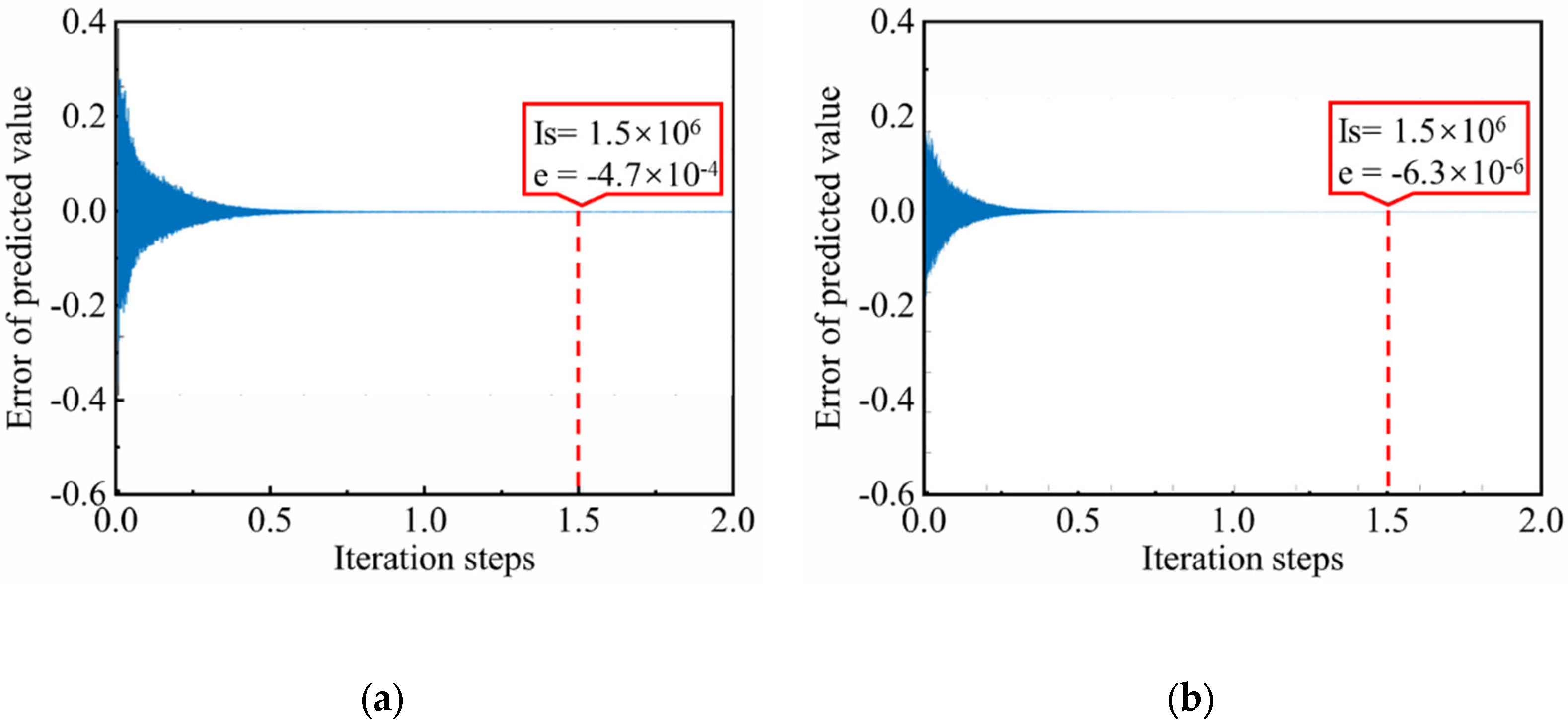
Figure 9 shows the variation in DD prediction total pressure and efficiency error with iteration steps (Is). When the number of iteration steps (Is) exceeds 1.5 × 10⁶, the error of prediction value (e) of ψOPT and ηOPT is reduced to −4.7 × 10⁻⁴ and −6.3 × 10⁻⁶, respectively. The prediction results are in complete agreement with the sample space, indicating that the calculation is convergent.
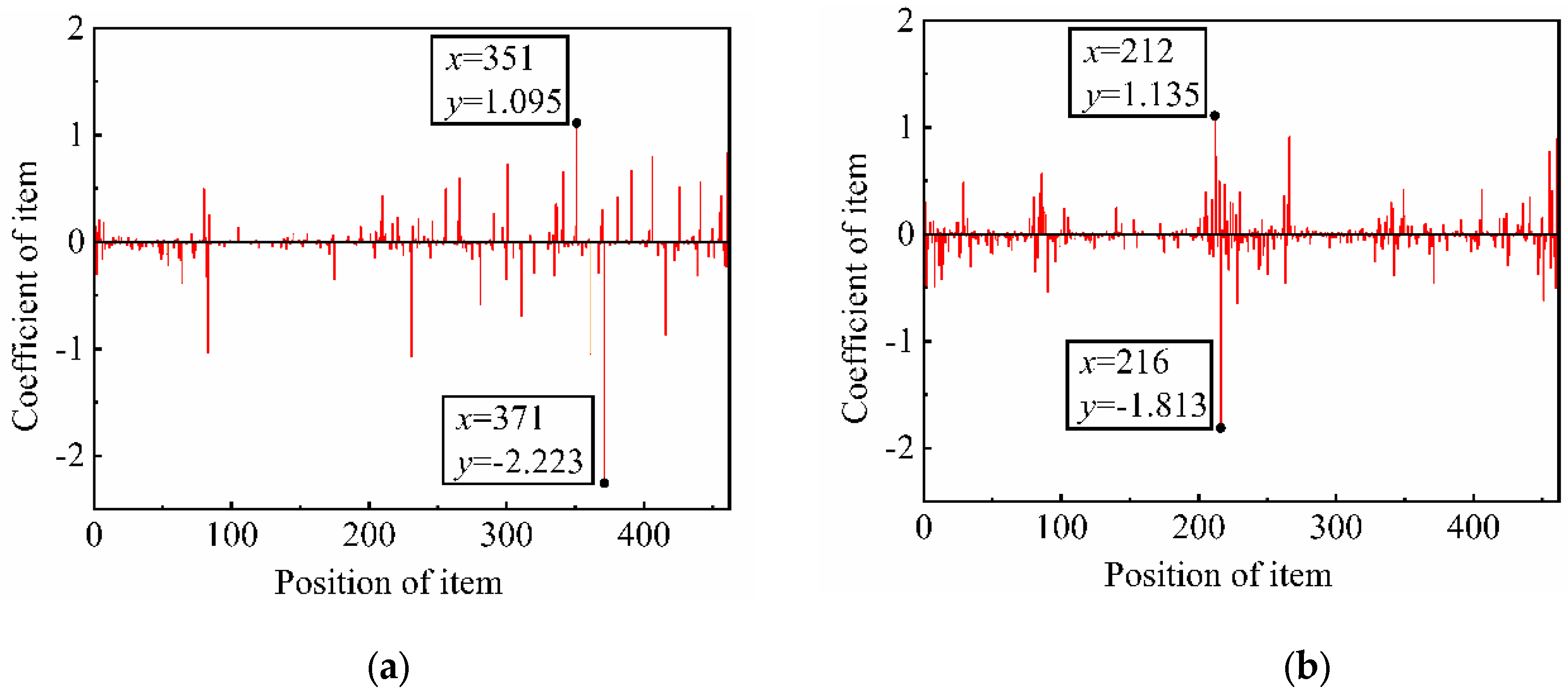
It is well known that the relationship between the inputs and outputs of the system can be expressed by the accumulation of the trigonometric function or polynomial. This study uses DD as a tool to transform the complex system into a polynomial. The relation spectrum shown in Figure 10 expresses the impact of the blade angle parameters on ψOPT and ηOPT, and the impact contains independent and interaction effects in different orders. The relation spectrum can be read by way of a checklist. “Position of items” corresponds to “Items” in Table 4. The relationship between blade angle parameters and ψOPT /ηOPT can be expressed as:
ψOPT = 0.154β05 − 0.301β04β1 + … + 0.253β0 + … − 0.269β14 + … + 1.095A3 + … − 2.223B2 − 0.111
ηOPT = 0.036β05 − 0.036β04β1 + … + 1.135β0 + … −1.813β14 + … − 0.011A3 + …− 0.462B2 + 0.242
According to the relation spectrum [28], the values of curve camber A and curve camber B have the most significant influence on the total pressure coefficient ψOPT. ψOPT is positively correlated to curve camber A but negatively correlated to curve camber B. As for the efficiency ηOPT, the most influential parameters are the blade angles in span 0 and span 1 (β0, β1). The ηOPT is positively correlated with β0 and negatively correlated with β1.
3.4. Optimization Algorithm
As there are two independent objectives in the optimization process of an axial fan, no single solution is globally optimal. For this reason, a multi-objective evolutionary algorithm is required to return a set of promising solutions. This study uses the non dominated sorting genetic algorithms with elite strategy (NSGA-II) to solve the global optimization problem [29]. We take the blade parameters (β0, β1, θ0, θ1, A, B) of the fan as optimization variables and the fan performance parameters (ψOPT, ηOPT) as the optimization objective. The two polynomials, trained to predict the fan performance parameters (ψOPT, ηOPT) in DD, are taken as the fitness function. The NSGA-II settings are shown in Table 5.
The constraint range of the optimization variables should generally be set based on the inherent parameters of the prototype scheme. However, according to the relationship spectrum, the performance parameters are sensitive to some blade parameters. In order to speed up the optimization process, the constrained range of the most critical parameters is modified based on the relation spectrum. The constrained range of blade parameters that are beneficial for the ψOPT and ηOPT, such as curve camber A and blade angles β0, are higher than those of the prototype. In contrast, the unfavorable blade parameters, such as curve camber B and blade angles β1, are lower than those of the prototype. The constraint range of the blade parameters is provided in Table 6.
We use the polynomial trained by DD to predict the fan performance parameters, which save computation time in the 3D numerical simulation. Thus, the population of the optimization algorithm can be appropriately increased to search the global optimization result. The population size is set at 500, and the algorithm evolution last for 200 generations. The convergence factor is defined to determine the convergence of the Pareto front as:
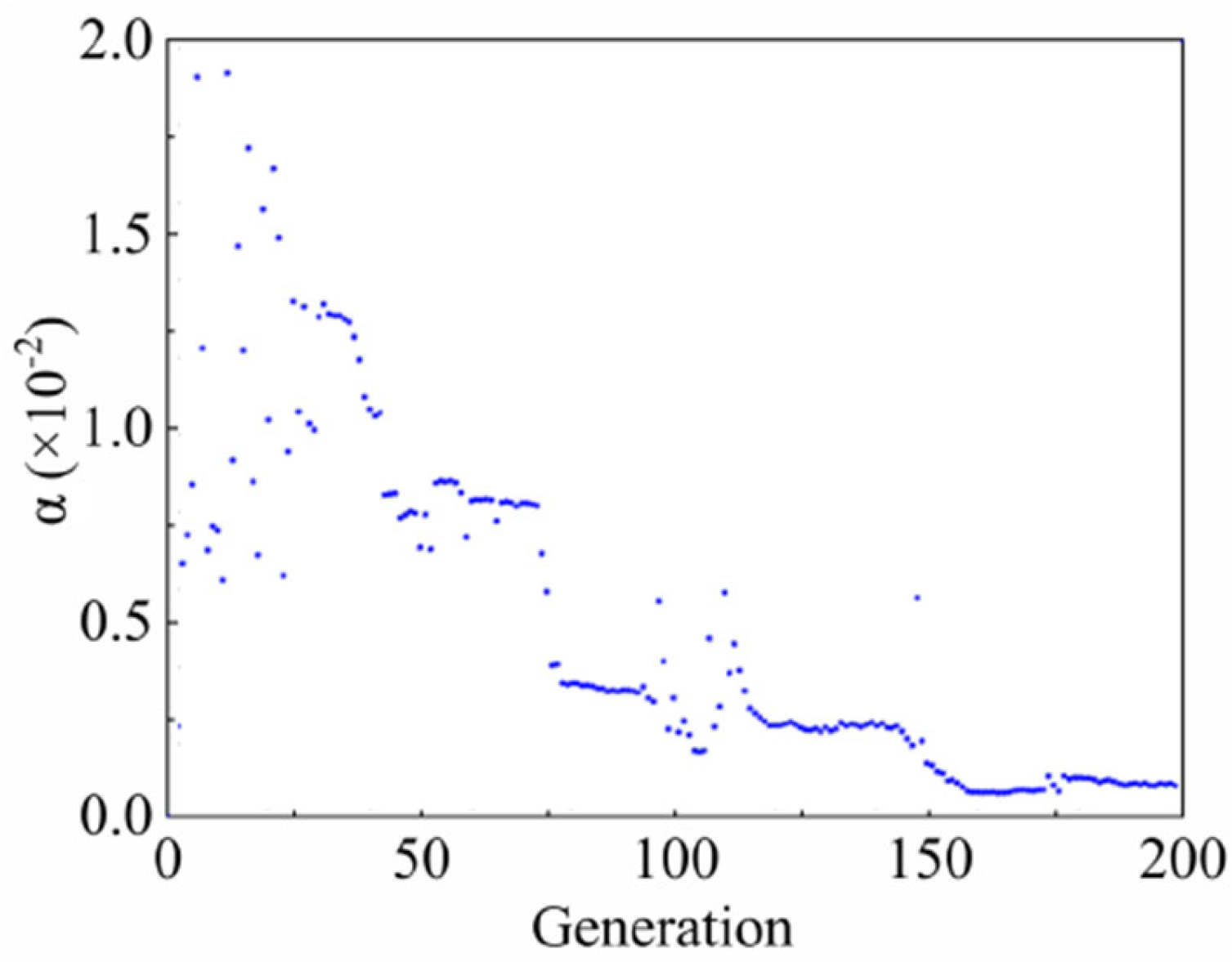
where is the kth dimension objective of the ith individual along the Pareto front in the tth generation population. The convergence factor α represents the average Euclidean distance between the leading-edge individual and the previous generation. Figure 11 shows the change in α with the evolution generation. As illustrated, α decreases rapidly in the first 100 generations, indicating that the objectives gradually converge in the process of crossover, mutation, and migration. After generation 130, the evolution slows down, and the α is reduced to 0.001.
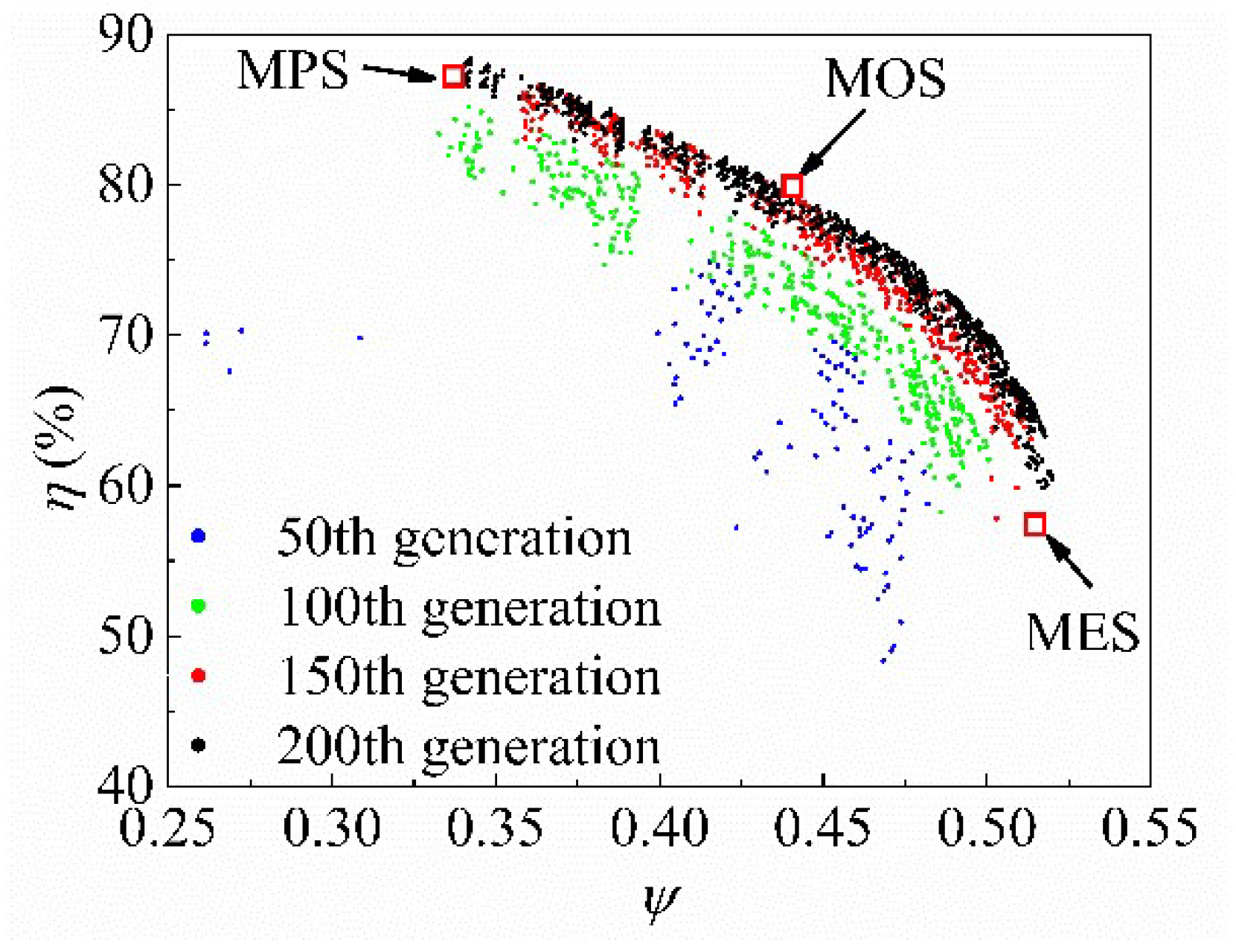
Figure 12 shows the Pareto front shape of the 50th, 100th, 150th, and 200th generations after transformation. As the initial population is randomly generated, the distribution position of the population at the 50th generation is relatively disorderly and scattered. When the evolution generation reaches 100, the Pareto front shape initially becomes an approximate arc. Then, the population distribution of the 150th generation moves to the upper right, and the spacing between individuals decreases. Finally, the distance between individuals further reduces in the 200th generation. As the Pareto front shape barely changes compared with the 150th generation, it can be assumed that the optimization process has converged.
The efficiency of the Pareto front ranges from 52.5% to 80.35%, and the pressure coefficient ranges from 0.38 to 0.56. A specific weight factor is generally needed to balance the two objectives to select the final scheme. As there is no apparent bias between pressure and efficiency in this optimization, the equal weight factors are adopted for the normalized efficiency and pressure coefficient. A scheme in the middle of the Pareto front is selected as the mean optimal scheme (MOS). Meanwhile, the maximum pressure scheme (MPS) and the maximum efficiency scheme (MES) are employed to analyze the internal flow variation compared with the original scheme (ORI).
4. Results and Analysis
4.1. Model and Parameter Comparison
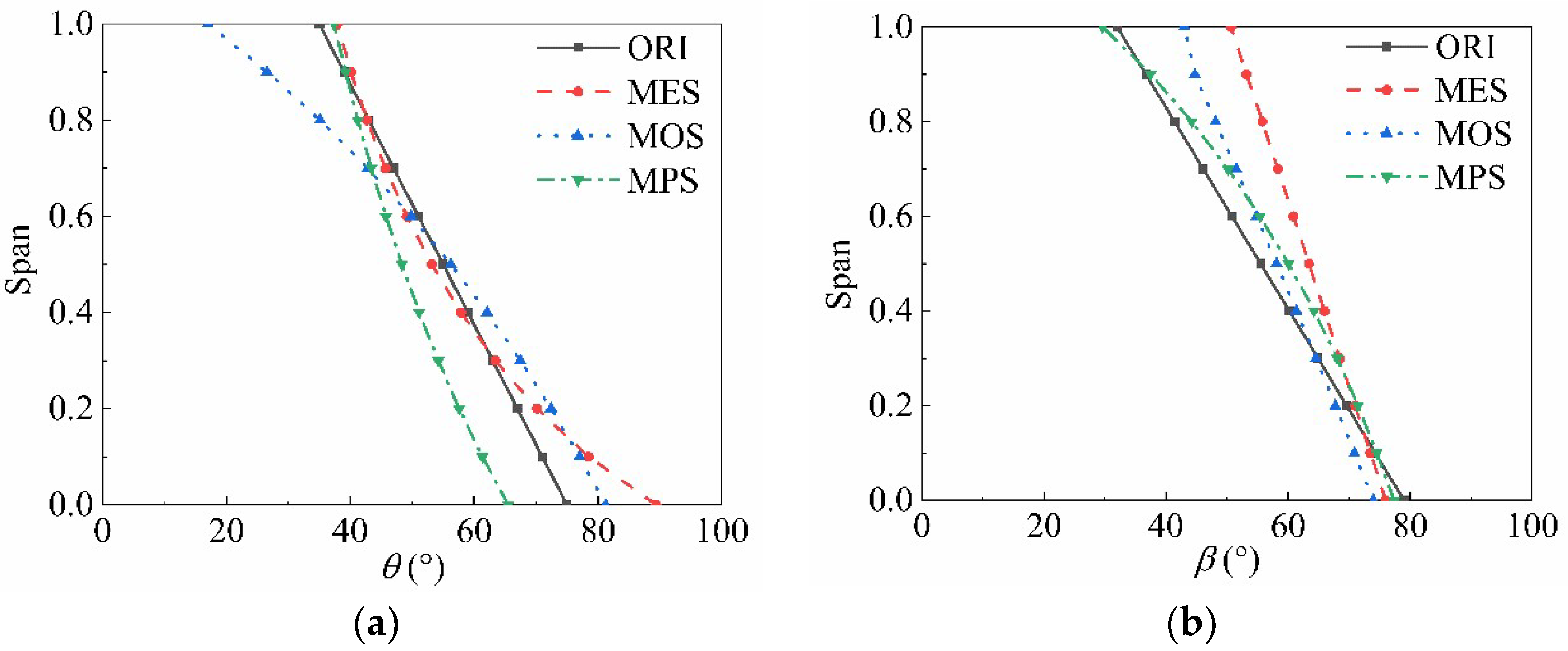
The distribution curves of θ and β along the spanwise direction are shown in Figure 13. The θ and β of the ORI linearly decrease with the impeller radius. Bézier curves are also used to construct the distribution of θ and β in the three optimization schemes. When the distribution is approximate to a concave function, the angle near the blade root section (span 0) changes rapidly. When the distribution is approximate to a convex function, the same angle change trend exists near the blade tip section (span 1).
Figure 14 shows the blade profiles of different schemes. The blade bending angle (θ) of the MES and MPS changes little along the spanwise direction under the three optimization schemes. Using the MOS, the blade bending angle decreases rapidly, making the arc at the top of the blade approximate a straight line. In addition, the maximum radial twist of blades exists in the MPS. Due to the rapid change in β at the blade tip, the blade twists most severely near the blade tip section (span 1). For MES and MOS, the change in β angle is approximately linear, and MES provides the minimum radial twist of blades.
4.2. Comparison of Blade Load
The models of the three optimization schemes are reconstructed, and the refined grid models are generated for numerical simulation to verify the optimization results. The static pressure loss coefficient is defined to describe the pressure distribution of different spanwise sections:
where is the static pressure on the blade surface, is the atmospheric pressure, and is the stagnation pressure at the leading edge of each spanwise section. It can be assumed that all spanwise sections experience constant stagnation pressure, ignoring the local blade geometry and flow condition.
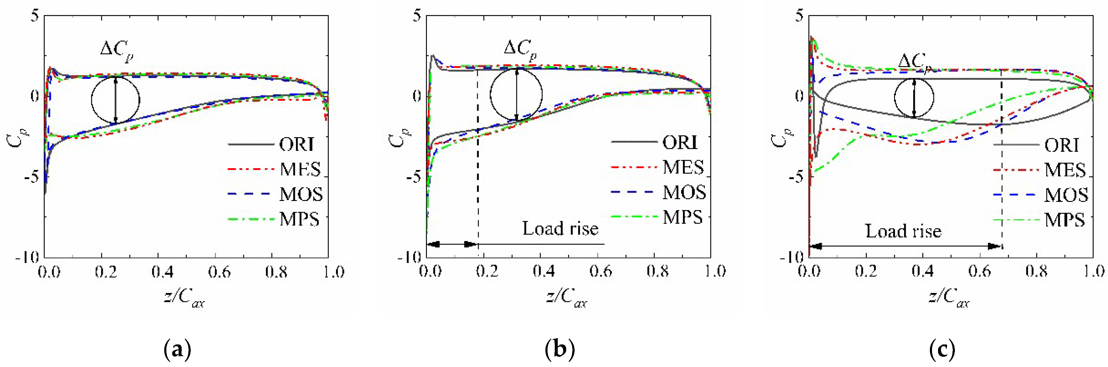
Figure 15 shows the distribution in three spanwise sections. The static pressure loss coefficient difference between the suction and pressure surface (ΔCp) represents the blade load in a specific relative chord position. At the blade root section (10% span), the distribution of different schemes shows a high coincidence. At the blade middle section (50% span), the ΔCp of the three optimal schemes slightly increases in the blade leading edge compared to the ORI, demonstrating that the blade load in this area is improved. At the blade middle section (90% span), the loading increase area extends to the middle of the blade, and the increase in blade load is enhanced.
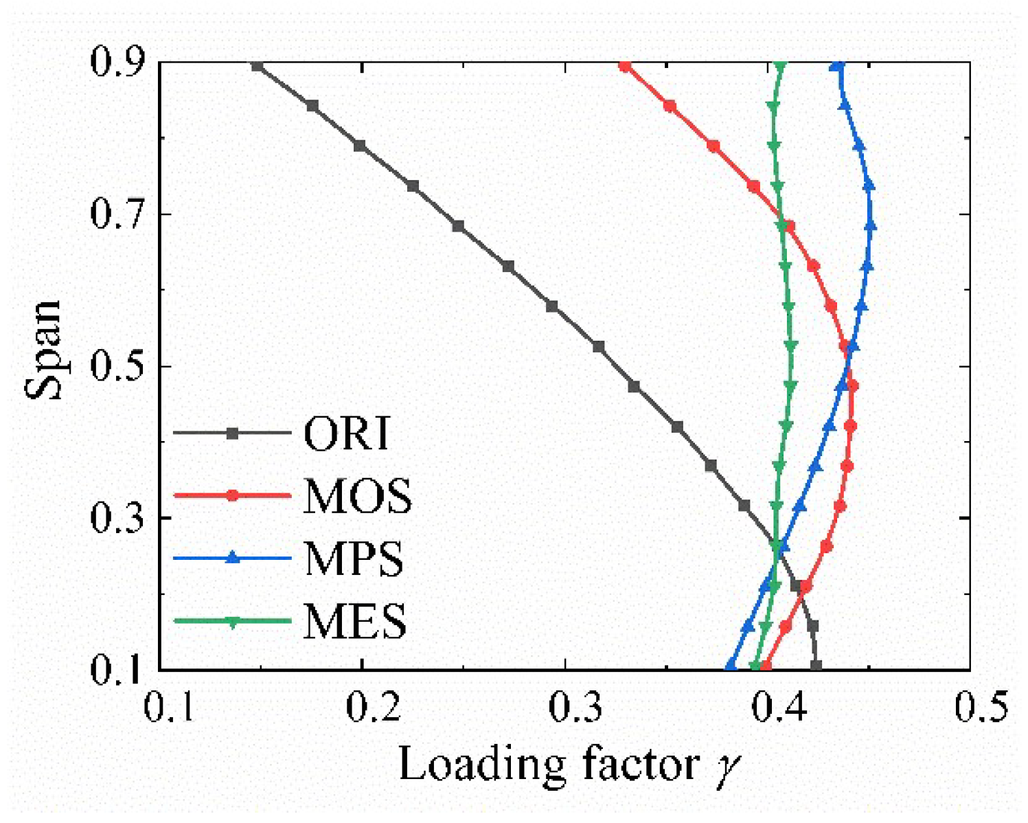
The results indicate that the new blade twist law leads to the redistribution of blade circumferential load. To further analyze blade load distribution along the span, the load factor γ is defined as follows:
where is the static pressure difference between the suction and pressure surface, and is the average axial velocity at the fan inlet. Figure 16 shows the blade load factor distribution along the spanwise direction. Among the four schemes, only the MES has a nearly linear distribution of the load factor. The load factor curves of ORI, MOS, and MPS show nonlinear shapes with different curvatures. The blade load decreases gradually along the spanwise direction for the ORI scheme, which indicates that the blade load concentrates on the blade area near the endwall. The blade load of the MES increases first and then decreases along the spanwise direction, and the maximum load point (MLP) is located at 45% of the span. For the MOS, the blade load factor distribution along the span is almost constant. The blade load of the MPS exhibits the same form as the MES, though the MLP moves to 65% of the span. It is noteworthy that the load distribution of all three optimized models is more uniform along the spanwise direction relative to the original scheme, and the MLP moves toward the middle of the blade.
4.3. Mechanism Analysis
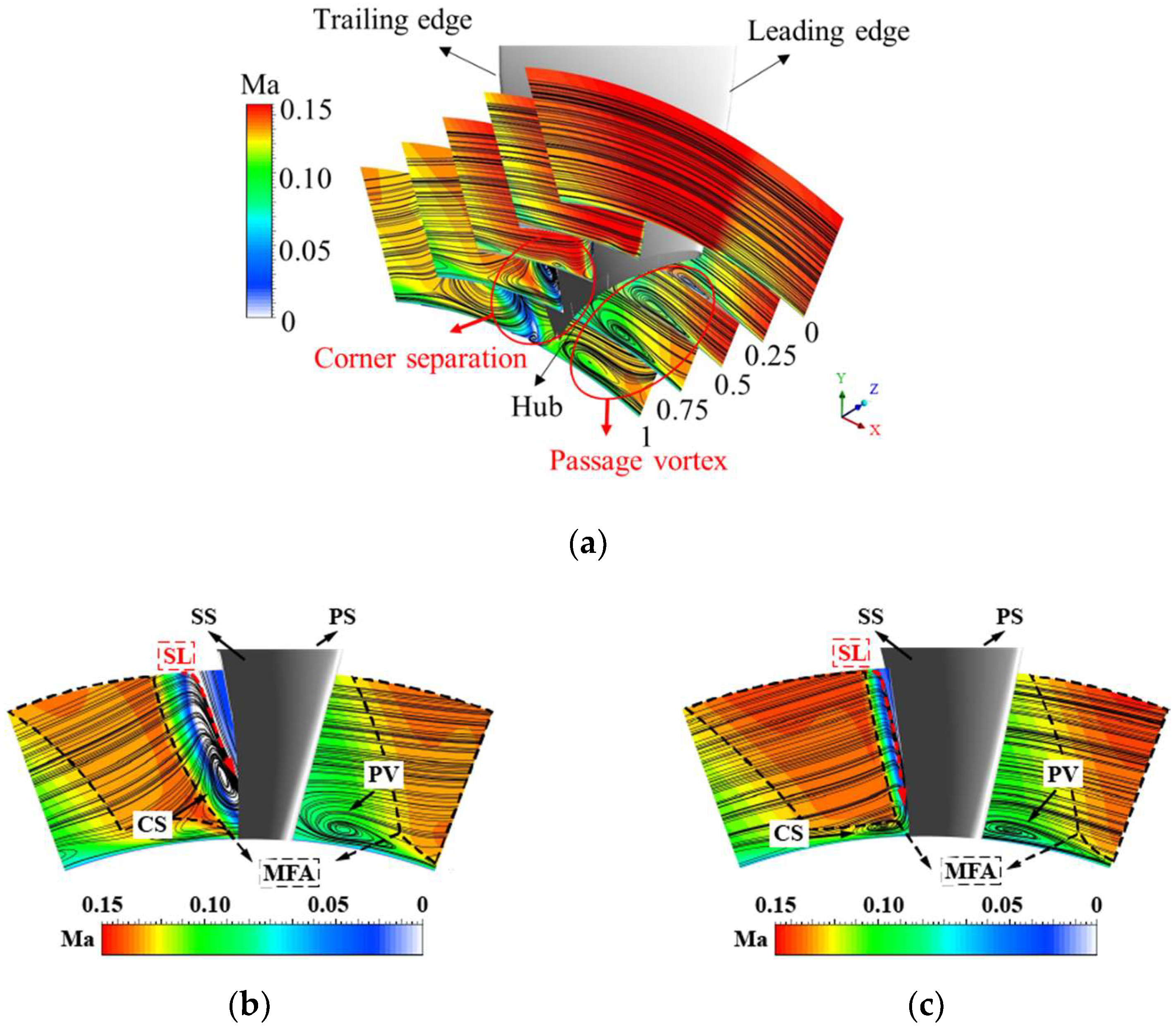
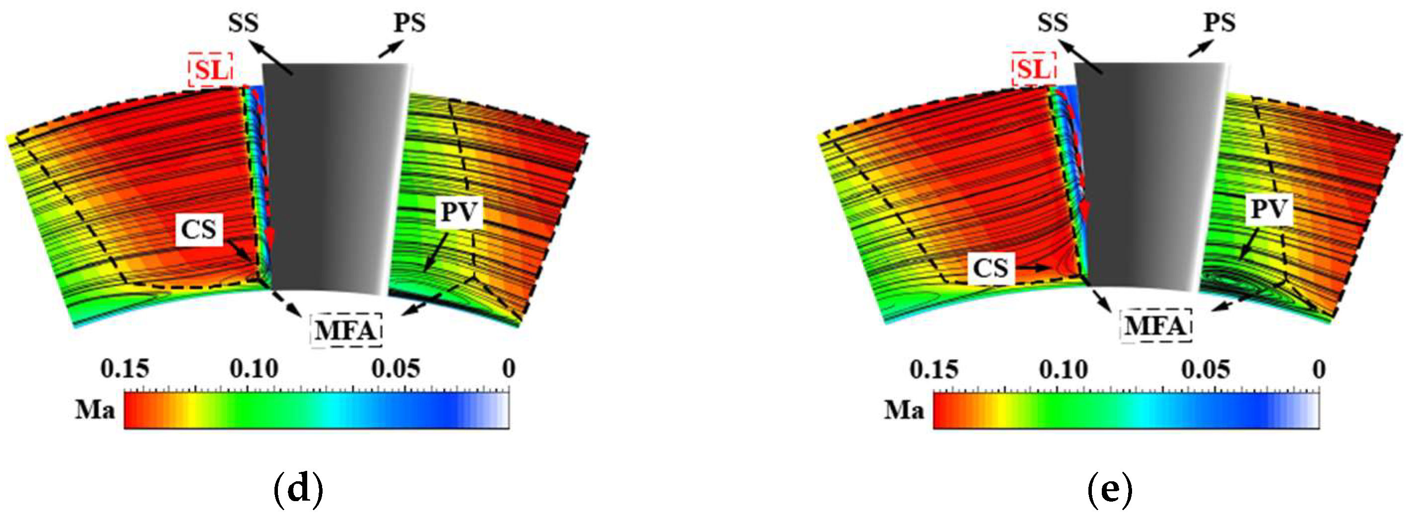
The streamline distribution and Mach contour near the endwall are provided in Figure 17 to illustrate the effect of the blade bending and twisting law. The rapid growth of the endwall boundary layer near the endwall and the secondary flow interaction lead to massive low-energy fluids localizing in the corner area, resulting in corner separation. Separation begins to form in the middle of the blade suction surface (z/Cax = 0.5) and develops continuously along the flow direction. A suction surface separation vortex (SSV) is formed near the suction surface of the ORI impeller at the trailing edge of the blade (z/Cax = 0.75). In the three optimized schemes, the separation line (SL) shifts to the suction side due to the uniform load distribution, and the separation vortex core is more inclined to the endwall, demonstrating that corner separation at the blade trailing edge is inhibited. In the adjacent passage, the centrifugal force in the mainstream fails to offset the pressure gradient, which leads to a flow separation near the endwall. The flow separation develops along the mainstream and generates a passage vortex (PV) at the blade trailing edge. Compared with the ORI impeller, the load changes more smoothly along the spanwise direction, which leads to a less adverse pressure gradient. The passage vortex (PV) of the three optimal schemes becomes narrow, and the flow velocity of the main flow area (MFA) increases. Most significantly, the redistribution of the blade load substantially restricts the flow separation and flow blockage near the endwall.
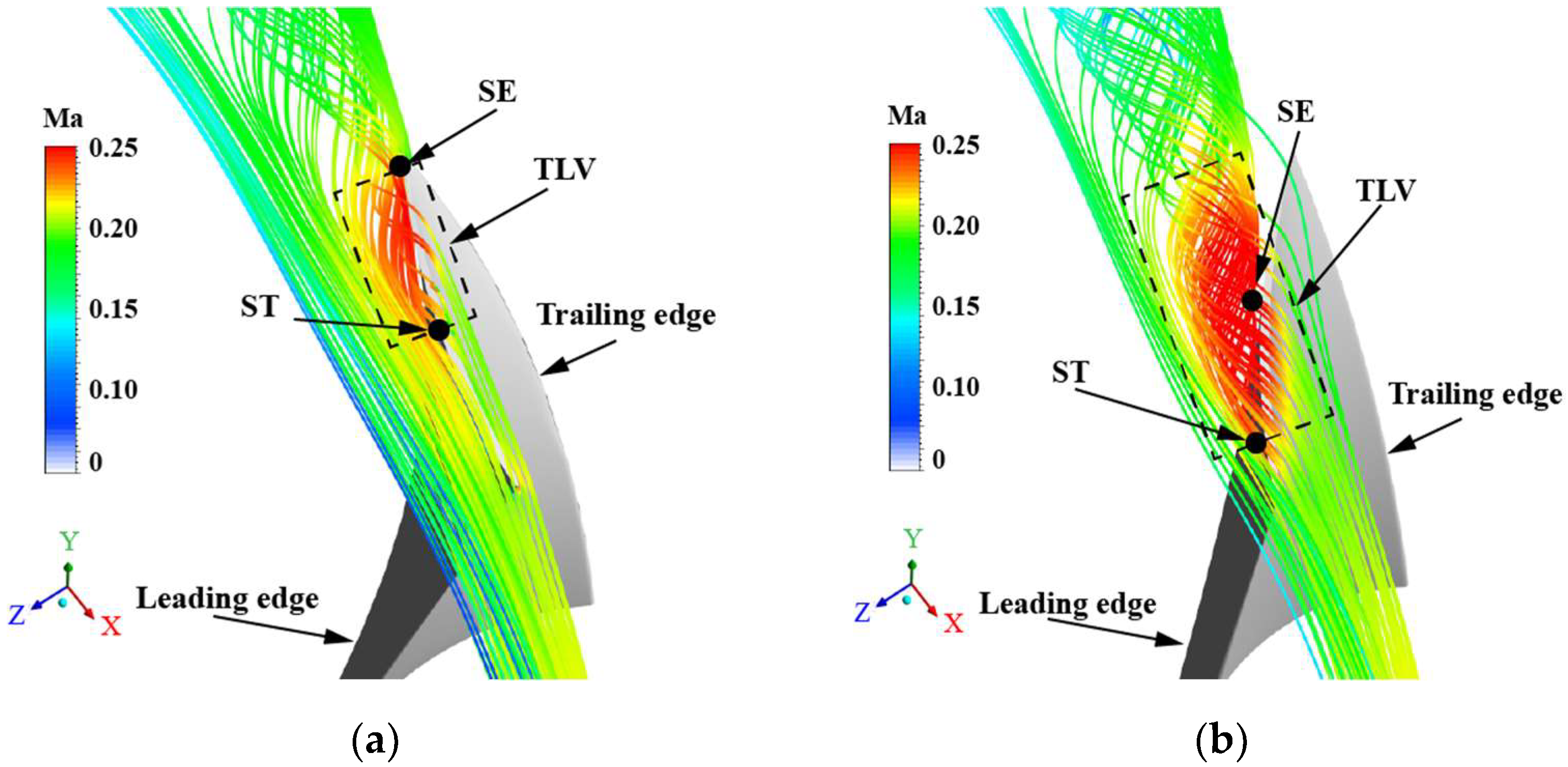
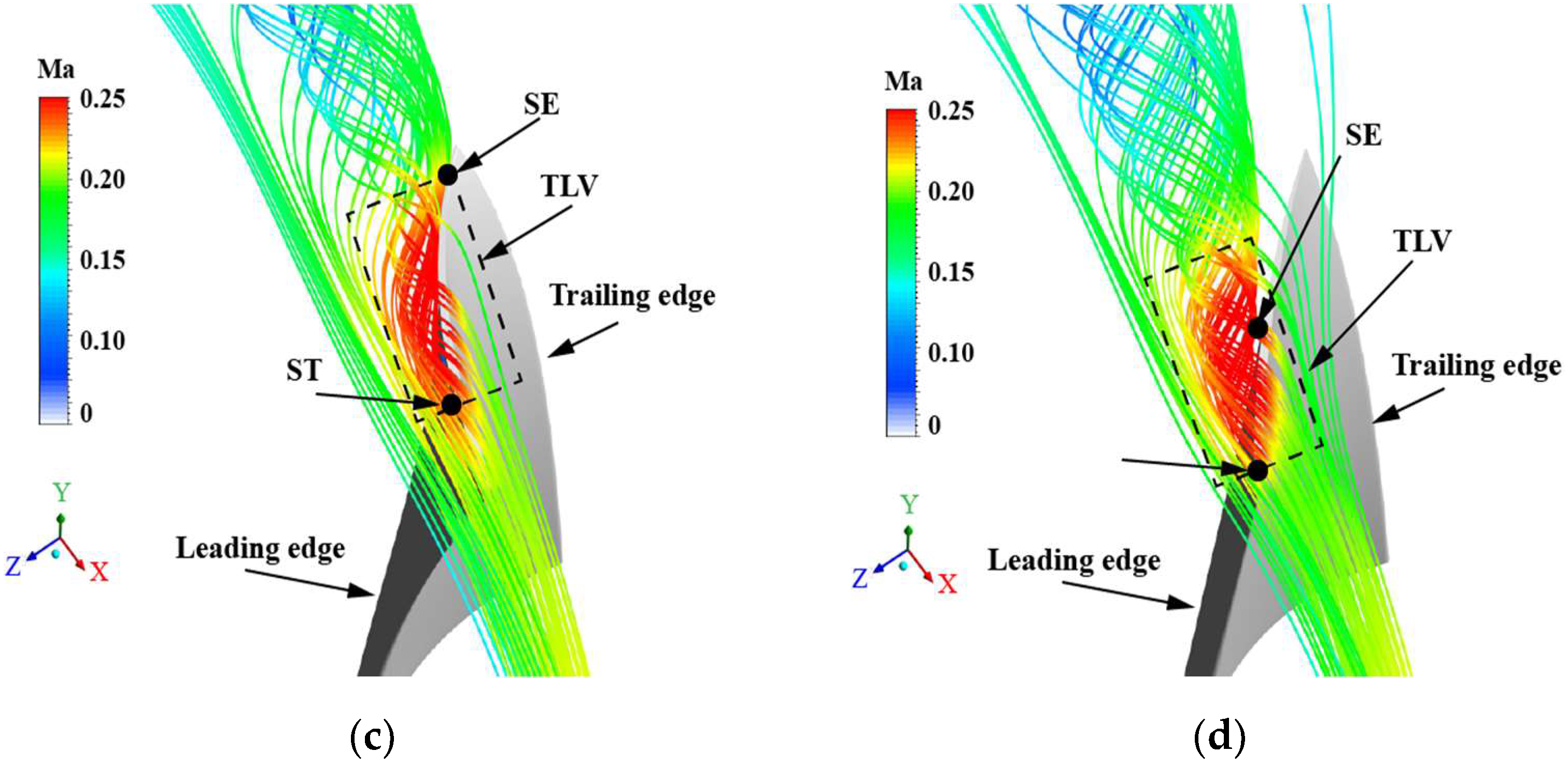
The new blade bending and twisting law imparts a smooth blade load distribution near the endwall. However, the blade tip load increases simultaneously. Figure 18 shows a comparison of the streamline at the tip clearance region. For the ORI impeller, a pressure difference between the suction and pressure side exists in the blade tip. The tip leakage vortex (TLV) is generated at the middle position of the blade and detaches at the trailing edge. After optimization, the pressure difference increases, indicating that the tip leakage vortex’s starting position (ST) and separation position (SE) have changed accordingly. The tip leakage vortex of the MES scheme starts from the middle of the blade. It develops along the blade suction surface and separates at the blade’s trailing edge. Tip leakage vortices in the MPS and MOS schemes are formed at the blade’s leading edge, separate from the blade surface near the middle of the blade suction surface.
4.4. Experimental Results
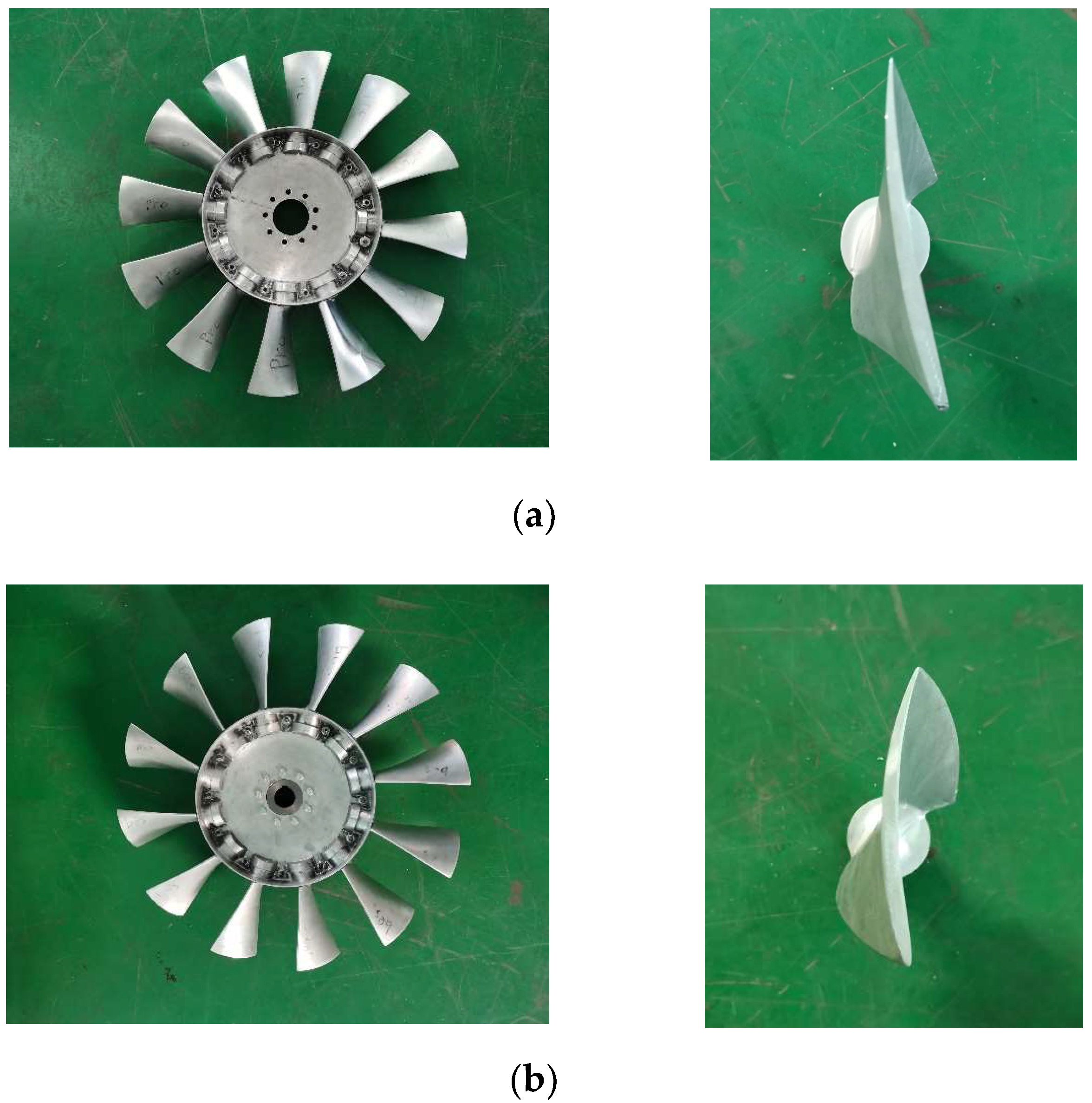
There is no apparent bias between the two optimization objectives of fan efficiency and total pressure in this study. Therefore, MOS is selected as the final scheme for our fan entity model. A comparison of the impeller models is shown in Figure 19. The aerodynamic characteristics are then tested on the pneumatic performance test bench shown in Figure 5.
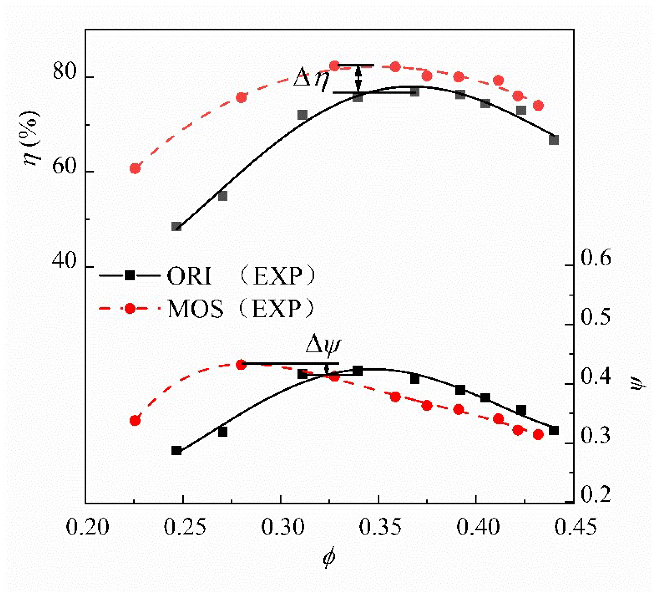
The total pressure and efficiency performance curves of the optimized and prototype fans are shown in Figure 20, indicating that the fan efficiency is improved under different flow rate conditions. The most significant improvement appears under the low-flow-rate condition, and the difference in fan efficiency before and after optimization decreases as flow rate increases. The maximum efficiency increases by 5.44%. On the other hand, the total pressure coefficient of the fan increases obviously at the low flow rate but is slightly lower than that of the prototype fan at the high flow rate. The maximum total pressure coefficient increases by 2.47%. In general, the MOS fan’s optimum working condition moves to the low-flow-rate zone. Combined with the previous analysis, the following explanation is given: The low-flow-rate condition approaches the stall point, which means the flow loss is mainly caused by the corner separation between the suction surface and endwall. Additionally, the flow separation in the corner area of the MOS fan is significantly suppressed after the redefinition of the blade bending and twisting law. As the flow rate increases, the flow velocity at the blade tip rises rapidly, leading to a severe tip leakage flow. After optimization, the load at the blade tip is enhanced, and the pressure difference between the pressure and suction surface increases. Tip leakage flow in the blade tip clearance is further aggravated, which induces the rapid reduction in fan efficiency and total pressure coefficient.
5. Conclusions
This study defined blade bending and twisting laws by changing the radial distribution of the blade angle and blade bending angle. A three-dimensional RANS simulation is then combined with the Dendrite Net to predict fan performance. The fan’s total pressure coefficient and efficiency are selected as the optimization objectives, and the NSGA-II algorithm is used to optimize the performance of the low-pressure axial flow fan.
The radial distribution of blade load can be influenced by changing the radial twist law of the blade. The blade angle parameters of the prototype fan are linearly distributed along the radial direction. Thus, the blade load is concentrated in the blade area near the endwall, which resulted in flow separation and passage vortex in the blade corner region. When the blade angle distribution is fitted reasonably by a Bézier curve, the load distribution along the radial direction is more uniform, and the maximum load point moved to the middle of the blade. Compared with the prototype fan, the suction surface separation vortex and passage vortex of the three optimal schemes are suppressed. On the other hand, the blade tip load of the three optimal schemes increased, which induced the tip leakage vortex to move towards the blade’s leading edge.
The mean optimal scheme (MOS) model is selected as the final scheme, and a pneumatic performance test is carried out. Compared to the prototype fan, the maximum efficiency increased by 5.44%, and the maximum total pressure coefficient increased by 2.47%. Thus, the optimum working condition of the MOS fan moved to a low-flow-rate zone.
Author Contributions
Conceptualization, Y.D. and J.W.; methodology, Y.D.; software, Y.D. and Q.X.; validation, L.W., B.X. and J.W.; formal analysis, Y.D. and Z.L.; investigation, Y.D.; resources, Q.X.; data curation, B.J.; writing—original draft preparation, Y.D.; writing—review and editing, Y.D.; visualization, Y.D.; supervision, J.W.; project administration, B.J. and L.W. All authors have read and agreed to the published version of the manuscript.
Funding
This research received no external funding.
Institutional Review Board Statement
Not applicable.
Informed Consent Statement
Not applicable.
Data Availability Statement
Not applicable.
Acknowledgments
The authors are deeply grateful for the provision of an experimental platform and assistance from the Nedfon Company, and the computing resources provided from SCTS/CGCL HPCC of HUST. The authors also appreciate all other scholars for their advice and assistance in improving this article.
Conflicts of Interest
The authors declare no conflict of interest.
Nomenclature
| DD | Readable polynomial neural network | θ | Blade bending angle |
| D0 | Shroud diameter | Flow coefficient | |
| Di | Hub diameter | Total pressure coefficient | |
| s/D0 | Tip-gap | Total pressure efficiency | |
| A | Camber of the θ distribution curve | Convergence factor | |
| B | Camber of the β distribution curve | ||
| Fan total pressure rise | Subscripts | ||
| Static pressure loss coefficient | 0 | Shroud side | |
| α | Load factor | 1 | Hub side |
| β | Blade angle | max | Maximum value |
| Qv | Volume flow rate | min | Minimum value |
References
- Li, C.; Li, X.; Li, P.; Ye, X. Numerical investigation of impeller trimming effect on performance of an axial flow fan. Energy 2014, 75, 534–548. [Google Scholar] [CrossRef]
- Pascu, M.; Miclea, M.; Epple, P.; Delgado, A.; Durst, F. Analytical and numerical investigation of the optimum pressure distribution along a low-pressure axial fan blade. Proc. Inst. Mech. Eng. Part C J. Mech. Eng. Sci. 2008, 223, 643–657. [Google Scholar] [CrossRef] [Green Version]
- Ye, X.; Li, P.; Li, C.; Ding, X. Numerical investigation of blade tip grooving effect on performance and dynamics of an axial flow fan. Energy 2015, 82, 556–569. [Google Scholar] [CrossRef]
- Pogorelov, A.; Meinke, M.; Schröder, W. Effects of tip clearance ratio width on the flow field in an axial fan. Int. J. Heat Fluid Flow 2016, 61, 466–481. [Google Scholar] [CrossRef]
- Rzadkowski, R.; Gnesin, V.; Kolodyzhnaya, L. 3D viscous flutter of 11th configuration Blade Row. Adv. Vib. Eng. 2009, 8, 213–221. [Google Scholar]
- Rzadkowski, R.; Gnesin, V.; Kolodyazhnaya, L.; Kubitz, L. Aeroelastic behaviour of a 3.5-stage aircraft compressor rotor blades following a bird strike. J. Vib. Eng. Technol. 2018, 6, 281–287. [Google Scholar] [CrossRef]
- Ghorbanian, K.; Gholamrezaei, M. Axial Compressor Performance Map Prediction Using Artificial Neural Network. In Proceedings of the ASME Turbo Expo 2007: Power for Land, Sea, and Air, Montreal, QC, Canada, 14 May 2007; pp. 1199–1208. [Google Scholar]
- Cortés, O.; Urquiza, G.; Hernández, J.A. Optimization of operating conditions for compressor performance by means of neural network inverse. Appl. Energy 2009, 86, 2487–2493. [Google Scholar] [CrossRef]
- Kamar, H.M.; Ahmad, R.; Kamsah, N.B.; Mohamad Mustafa, A.F. Artificial neural networks for automotive air-conditioning systems performance prediction. Appl. Therm. Eng. 2013, 50, 63–70. [Google Scholar] [CrossRef]
- Herrig, L.J.; Emery, J.C.; Erwin, J.R. Systematic Two-Dimensional Cascade Tests of NACA 65-Series Compressor Blades at Low Speeds; UNT Digital Library: Denton, TX, USA, 1957. [Google Scholar]
- Han, X.-A.; Ma, Y.; Huang, X. A novel generalization of Bézier curve and surface. J. Comput. Appl. Math. 2008, 217, 180–193. [Google Scholar] [CrossRef] [Green Version]
- Farin, G. Algorithms for rational Bézier curves. Comput. -Aided Des. 1983, 15, 73–77. [Google Scholar] [CrossRef]
- Jiang, B.; Wang, J.; Yang, X.; Wang, W.; Ding, Y. Tonal noise reduction by unevenly spaced blades in a forward-curved-blades centrifugal fan. Appl. Acoust. 2019, 146, 172–183. [Google Scholar] [CrossRef]
- Xiao, Q.; Shi, X.; Wu, L.; Wang, J.; Ding, Y.; Jiang, B. Squirrel-Cage Fan System Optimization and Flow Field Prediction Using Parallel Filling Criterion and Surrogate Model. Processes 2021, 9, 1620. [Google Scholar] [CrossRef]
- Xia, G.; Medic, G.; Praisner, T.J. Hybrid RANS/LES Simulation of Corner Stall in a Linear Compressor Cascade. J. Turbomach. 2018, 140, 081004. [Google Scholar] [CrossRef]
- Bamberger, K.; Carolus, T. Development, Application, and Validation of a Quick Optimization Method for the Class of Axial Fans. J. Turbomach. 2017, 139, 111001. [Google Scholar] [CrossRef]
- ISO 5801; Fans—Performance Testing Using Standardized Airways. ISO: London, UK, 2017.
- Yang, X.; Jiang, B.; Wang, J.; Huang, Y.; Yang, W.; Yuan, K.; Shi, X. Multi-objective optimization of dual-arc blades in a squirrel-cage fan using modified non-dominated sorting genetic algorithm. Proc. Inst. Mech. Eng. Part A J. Power Energy 2020, 234, 1053–1068. [Google Scholar] [CrossRef]
- Wang, W.; Wang, J.; Liu, H.; Jiang, B.-Y. CFD Prediction of Airfoil Drag in Viscous Flow Using the Entropy Generation Method. Math. Probl. Eng. 2018, 2018, 4347650. [Google Scholar] [CrossRef] [Green Version]
- Brunet, V.; Croner, E.; Minot, A.; de Laborderie, J.; Lippinois, E.; Richard, S.; Renac, F. Comparison of Various CFD Codes for LES Simulations of Turbomachinery: From Inviscid Vortex Convection to Multi-Stage Compressor. In Proceedings of the ASME Turbo Expo 2018: Turbomachinery Technical Conference and Exposition, Lillestrøm, Norway, 11–15 June 2018. [Google Scholar]
- Nazmi Ilikan, A.; Ayder, E. Influence of the Sweep Stacking on the Performance of an Axial Fan. J. Turbomach. 2015, 137, 061004. [Google Scholar] [CrossRef]
- Rosin, C.D.; Belew, R.K. New methods for competitive coevolution. Evol. Comput. 1997, 5, 1–29. [Google Scholar] [CrossRef]
- Steinberg, D.M.; Lin, D.K.J. A construction method for orthogonal Latin hypercube designs. Biometrika 2006, 93, 279–288. [Google Scholar] [CrossRef]
- Liu, G.; Wang, J. Dendrite Net: A White-Box Module for Classification, Regression, and System Identification. arXiv 2020, arXiv:2004.03955. [Google Scholar] [CrossRef]
- Deb, K.; Agrawal, S.; Pratap, A.; Meyarivan, T. A fast elitist non-dominated sorting genetic algorithm for multi-objective optimization: NSGA-II. In Parallel Problem Solving from Nature PPSN VI, Proceedings of the International Conference on Parallel Problem Solving from Nature, Paris, France, 18–20 September 2000; Springer: Berlin/Heidelberg, Germany, 2000; pp. 849–858. [Google Scholar]
- Rumelhart, D.E.; Hinton, G.E.; Williams, R.J. Learning representations by back-propagating errors. Nature 1986, 323, 533–536. [Google Scholar] [CrossRef]
- Dyall, K.G. Interfacing relativistic and nonrelativistic methods. I. Normalized elimination of the small component in the modified Dirac equation. J. Chem. Phys. 1997, 106, 9618–9626. [Google Scholar] [CrossRef]
- Zhang, J.; Zhu, H.; Yang, C.; Li, Y.; Wei, H. Multi-objective shape optimization of helico-axial multiphase pump impeller based on NSGA-II and ANN. Energy Convers. Manag. 2011, 52, 538–546. [Google Scholar] [CrossRef]
- Zhang, W.; Yuan, J.; Si, Q.; Fu, Y. Investigating the In-Flow Characteristics of Multi-Operation Conditions of Cross-Flow Fan in Air Conditioning Systems. Processes 2019, 7, 959. [Google Scholar] [CrossRef] [Green Version]
Figure 1.
Schematic diagram of the prototype fan: (a) 3D model of the prototype fan; (b) schematic diagram of the pipeline system.
Figure 1.
Schematic diagram of the prototype fan: (a) 3D model of the prototype fan; (b) schematic diagram of the pipeline system.

Figure 2.
Axial flow fan blade modeling method: (a) 3D impeller model and the position of θ and β; (b) the radial distribution of θ and β.
Figure 2.
Axial flow fan blade modeling method: (a) 3D impeller model and the position of θ and β; (b) the radial distribution of θ and β.

Figure 3.
Computing domain of the axial flow fan.

Figure 4.
Mesh model of the axial flow fan: (a) the impeller and deflector; (b) the blade; (c) Boundary layer.
Figure 4.
Mesh model of the axial flow fan: (a) the impeller and deflector; (b) the blade; (c) Boundary layer.

Figure 5.
Aerodynamic performance experimental setup: (a) schematic diagram of experimental system, 1. rectifying device, 2. expansion tube, 3. expansion tube; (b) field diagram of experimental device.
Figure 5.
Aerodynamic performance experimental setup: (a) schematic diagram of experimental system, 1. rectifying device, 2. expansion tube, 3. expansion tube; (b) field diagram of experimental device.


Figure 6.
Variation in experimental and calculated performance curves: (a) performance curve of total pressure; (b) performance curve of total efficiency.
Figure 6.
Variation in experimental and calculated performance curves: (a) performance curve of total pressure; (b) performance curve of total efficiency.

Figure 7.
Optimization process.

Figure 8.
Graphical illustration of learning rules.

Figure 9.
The variation in prediction error with iteration steps: (a) total pressure training error; (b) efficiency training error.
Figure 9.
The variation in prediction error with iteration steps: (a) total pressure training error; (b) efficiency training error.

Figure 10.
The relation spectrum: (a) the relation spectrum of total pressure coefficient; (b) the relation spectrum of efficiency.
Figure 10.
The relation spectrum: (a) the relation spectrum of total pressure coefficient; (b) the relation spectrum of efficiency.

Figure 11.
The variation in convergence factor with the evolution generation.

Figure 12.
The Pareto front shape of different generations.

Figure 13.
The distribution curves of θ and β along the spanwise direction: (a) the radial distribution of θ; (b) the radial distribution of β.
Figure 13.
The distribution curves of θ and β along the spanwise direction: (a) the radial distribution of θ; (b) the radial distribution of β.

Figure 14.
Comparison of blade profile and 3D modeling: (a) ORI; (b) MES; (c) MOS; (d) MPS.

Figure 15.
Cp distribution in the spanwise sections of 10%, 50%, and 90% span: (a) 10% of span; (b) 50% of span; (c) 90% of span.
Figure 15.
Cp distribution in the spanwise sections of 10%, 50%, and 90% span: (a) 10% of span; (b) 50% of span; (c) 90% of span.

Figure 16.
Load factor distribution along the spanwise direction.

Figure 17.
Comparison of streamline distribution and Mach contour near the endwall: (a) flow characteristic near the endwall; (b) ORI; (c) MES; (d) MOS; (e) MPS.
Figure 17.
Comparison of streamline distribution and Mach contour near the endwall: (a) flow characteristic near the endwall; (b) ORI; (c) MES; (d) MOS; (e) MPS.


Figure 18.
Comparison of tip leakage vortices: (a) ORI; (b) MES; (c) MOS; (d) MPS.


Figure 19.
Comparison of impeller models: (a) ORI model impeller; (b) MOS model impeller.

Figure 20.
Experimental performance curves of optimized and prototype fans.


Table 1.
Main parameters of the original axial fan.
| Parameter | Value |
|---|---|
| Rotor speed n (RPM) | 1450 |
| Number of impeller blades Zi | 12 |
| Number of deflector blades Zd | 17 |
| Shroud diameter (D0/mm) | 800 |
| Hub diameter (Di/mm) | 410 |
| Blade chord (Ca/mm) | 95 |
| Tip clearance ratio (s/D0) | 0.625% |
Table 2.
Grid quantity distribution.
| Flow Area | Inlet Extension | Impeller | Deflector | Outlet Extension | Total |
|---|---|---|---|---|---|
| Grid 1 | 1.66 × 10⁶ | 2.83 × 10⁶ | 1.03 × 10⁶ | 0.84 × 10⁶ | 6.36 × 10⁶ |
| Grid 2 | 2.34 × 10⁶ | 3.64 × 10⁶ | 1.53 × 10⁶ | 1.02 × 10⁶ | 8.53 × 10⁶ |
| Grid 3 | 3.05 × 10⁶ | 4.96 × 10⁶ | 1.89 × 10⁶ | 1.10 × 10⁶ | 11.02 × 10⁶ |
| Grid 4 | 3.6 × 10⁶ | 5.55 × 10⁶ | 2.45 × 10⁶ | 1.86 × 10⁶ | 13.28 × 10⁶ |
Table 3.
Initial sample space.
| X | Y1 | Y2 | |||||
|---|---|---|---|---|---|---|---|
| β0 | β1 | a | θ0 | θ1 | b | ψOPT | ηOPT |
| 82 | 31 | 0.19 | 57 | 35 | 0.25 | 0.38 | 74.77 |
| 89 | 38 | 0.30 | 76 | 51 | −0.01 | 0.38 | 74.15 |
| 67 | 30 | −0.07 | 75 | 24 | −0.17 | 0.47 | 75.02 |
| … | |||||||
| 95 | 24 | −0.04 | 79 | 38 | 0.05 | 0.45 | 76.33 |
Table 4.
Position of Item.
| Position (x) | Weight of ψOPT (yψ) | Weight of ηOPT (yη) | Item |
|---|---|---|---|
| 1 | 0.154 | 0.036 | β05 |
| 2 | −0.301 | −0.036 | β04β1 |
| … | |||
| 212 | 0.253 | 1.135 | β0 |
| … | |||
| 216 | −0.269 | −1.813 | β14 |
| … | |||
| 351 | 1.095 | −0.011 | A3 |
| … | |||
| 371 | −2.223 | −0.462 | B2 |
| … | |||
| 462 | −0.111 | 0.242 | 1 |
Table 5.
Specific parameter settings of NSGA-II.
| Options | Parameters |
|---|---|
| Number of variables | 6 |
| Population size | 500 |
| Selection function | Tournament |
| Mutation function | Uniform |
| Crossover function | Scattered |
| Migration direction | Forward |
| Stopping generation | 200 |
Table 6.
Constraint range of blade parameters.
| Design Variable | Variable Name | Range |
|---|---|---|
| Var 1 | β0 | (65, 95) |
| Var 2 | β1 | (15, 45) |
| Var 3 | θ0 | (55, 95) |
| Var 4 | θ1 | (12, 52) |
| Var 5 | A | (0, 0.3) |
| Var 6 | B | (−0.3, 0) |
Publisher’s Note: MDPI stays neutral with regard to jurisdictional claims in published maps and institutional affiliations. |
© 2022 by the authors. Licensee MDPI, Basel, Switzerland. This article is an open access article distributed under the terms and conditions of the Creative Commons Attribution (CC BY) license (https://creativecommons.org/licenses/by/4.0/).
Share and Cite
MDPI and ACS Style
Ding, Y.; Wang, J.; Jiang, B.; Li, Z.; Xiao, Q.; Wu, L.; Xie, B. Multi-Objective Optimization for the Radial Bending and Twisting Law of Axial Fan Blades. Processes 2022, 10, 753. https://0-doi-org.brum.beds.ac.uk/10.3390/pr10040753
AMA Style
Ding Y, Wang J, Jiang B, Li Z, Xiao Q, Wu L, Xie B. Multi-Objective Optimization for the Radial Bending and Twisting Law of Axial Fan Blades. Processes. 2022; 10(4):753. https://0-doi-org.brum.beds.ac.uk/10.3390/pr10040753
Chicago/Turabian StyleDing, Yanyan, Jun Wang, Boyan Jiang, Zhiang Li, Qianhao Xiao, Lanyong Wu, and Bochao Xie. 2022. "Multi-Objective Optimization for the Radial Bending and Twisting Law of Axial Fan Blades" Processes 10, no. 4: 753. https://0-doi-org.brum.beds.ac.uk/10.3390/pr10040753
Note that from the first issue of 2016, this journal uses article numbers instead of page numbers. See further details here.