
Estimation of Reverse Flow Rate in J-Groove Channel of AJP and SCP Models Using CFD Analysis


1
Graduate School of Mechanical Engineering, Mokpo National University, Muan 58554, Korea
2
Department of Mechanical Engineering, Institute of New and Renewable Energy Technology Research, Mokpo National University, Muan 58554, Korea
*
Author to whom correspondence should be addressed.
Processes 2022, 10(4), 785; https://0-doi-org.brum.beds.ac.uk/10.3390/pr10040785
Submission received: 11 March 2022
/
Revised: 9 April 2022
/
Accepted: 13 April 2022
/
Published: 16 April 2022
(This article belongs to the Special Issue CFD Based Researches and Applications for Fluid Machinery and Fluid Device, Volume II)
Abstract
:An annular jet pump (AJP) and a screw centrifugal pump (SCP) are special-purpose pumps used for transportation. The flow fields in the AJP and SCP are like those in a diffuser without and with an impeller, respectively. The flow from diffuser inlet to outlet takes place via the conversion of kinetic energy to static pressure. J-Groove is installed in the diffuser wall of an AJP and SCP to induce reverse flow from the diffuser outlet to the inlet, which suppresses the cavitation. CFD analysis was carried out to verify the conceptual design and understand the internal flow field of an AJP and SCP with J-Groove. The CFD analysis showed that the J-Groove installation in the AJP and SCP improved suction performance. The reverse flow in the J-Groove is due to the pressure difference between the diffuser outlet and the inlet. The numerical analysis results showed that the reverse flow mechanism is dependent on the flow conditions, cavitation number, and presence of the impeller. In a higher flow rate, the reverse flow rate is higher in the AJP model and lower in the SCP model and vice versa. Finally, CFD analysis concluded that the reverse flow rate in J-Groove improves the suction performance of the AJP and SCP models.
1. Introduction
With the growth in the agriculture and aquaculture industry, the demand for transportation pumps has increased. The pumps can be efficient and effective substitutes for transportation. Among various pump categories, jet pumps and screw centrifugal pumps are used in sewage transfer, petroleum, metallurgy, and other industries for transportation [1,2]. Therefore, jet pumps and centrifugal pumps are the most viable options to solve the transportation problem of sensitive goods such as vegetables and live fish.
Jet pumps are preferred for transportation because they are simple in design without rotating and reciprocating components, low cost, and have desirable mass transfer [3,4]. The primary and secondary inlets, nozzle, diffuser, and outlet are the main components of a jet pump. A jet pump converts pressure energy into kinetic energy using a nozzle and diffuser. The high pressurized primary flow passes through the nozzle and increases the fluid velocity, which creates a low-pressure zone in the throat and withdraws secondary fluid. Finally, the high-pressure primary fluid mixes with low-pressure secondary fluid at the throat and diffuses to the outlet via a diffuser [5]. The drawbacks of the jet pump are friction loss, mixing loss, and the possibility of cavitation. Generally, two types of jet pump are available in the market, central jet pump (CJP) and annular jet pump (AJP) [6]. The nozzle position distinguishes between CJPs and AJPs. In CJPs, the primary pressurized fluid passes through the central nozzle, whereas in AJPs, the pressurized fluid passes through the annular nozzle. Numerous studies [7,8,9] were conducted on the design and operation of CJPs. Hatzlavramidis [7] proposed the design methodology to model CJPs. The CJP performance is dependent on the nozzle shape, size, and number [8]. Zhu et al. [9] established the computational methodology for the design and engineering practice of CJPs.
Hence, an AJP is selected to improve the suction performance for the transfer of sensitive goods. Shimizu et al. [10] conducted the experimental analysis on various AJP geometry configurations to evaluate hydraulic and suction performance. Elger et al. [6] introduced dimensionless parameters to study the recirculation flow in an AJP. AJP performance is directly related to the nozzle shape and size [11]. Kwon et al. [12] conducted numerical analysis on an AJP and showed that recirculation mainly occurs under partial flow conditions. Numerical analysis showed that AJPs are more efficient in transportation [13].
The screw centrifugal pump (SCP) is used for slurries, sewage, and sensitive goods transfer. The SCP has a large and open channel from suction to discharge, which helps to transfer the solid particles without clogging. SCPs have a three-dimensional spiral blade added to the conical hub cone. It is the combination of screw pump and centrifugal pump which provides spiral propeller and centrifugal effects, respectively [14]. The higher efficiency, no blockage area, a wide range of operation, and better solid handling capability are the advantages of screw centrifugal pumps over traditional slurry pumps [15]. Few studies were conducted to understand the SCP. The meridional shape parameters of the screw centrifugal pump influence the performance and internal flow [16]. The axial thrust becomes larger where the impeller radius reaches the tongue of the volute casing [17]. Cheng et al. [18] explained the parametric equation for the design of the SCP impeller blade. Guo et al. [19] showed the design method and internal flow behavior of the SCP.
The cavitation occurrence is the main problem for the proper operation of the AJP and the SCP. Cavitation vapor bubbles occur in the nozzle of the AJP and inlet of the SCP impeller blade when they operate below the saturated vapor pressure. The cavitation reduces the pump efficiency and damages the transported goods. The instability of the re-entrant jet and pressure gradient in the re-entrant jet creates cloud cavitation in the divergence section of the AJP [20]. Xiao et al. [21] conducted cavitation analysis in the AJP. Cavitation in the AJP can be caused by increasing the primary jet velocity or decreasing pump outlet pressure [22]. The cavitation phenomenon in the SCP is like in the centrifugal pump and is caused by reducing the inlet pressure. Backflow vortex cavitation and tip leakage cavitation occur at the impeller inlet of the SCP. Cavitation in the AJP and SCP is dependent on the flow condition. Cavitation causes severe damage to sensitive goods such as fish [23]. The improvement of pressure distribution will suppress cavitation in the AJP and the SCP.
The flow field in the AJP and SCP models are alike as a diffuser without and with an impeller, respectively. The diffuser is a pressure-momentum device that focuses on recovering static pressure at the expense of kinetic energy [24]. The static pressure recovery coefficient for the diffuser is calculated as
where is static pressure (Pa), is dynamic pressure (Pa), is velocity (m/s), is the density of fluid (kg/m3), is the pressure recovery coefficient, and subscripts 1 and 2 represent the inlet and outlet of the diffuser.
J-Groove is a simple passive approach to suppress cavitation in the diffuser of AJP and the impeller wall of the SCP [25,26]. It induces the reverse jet flow and suppresses cavitation in the diffuser wall [27]. The main design parameters for J-Groove are depth, length, angle, and number [28], and its depth plays a vital role in the reverse flow rate and suction performance improvement [29].
The flow in J-Groove is dependent on the pressure difference. In a diffuser , it directs the flow in the J-Groove from the outlet to the inlet of the diffuser. Hence, a reverse flow can be observed in the diffuser with J-Groove. This study is focused on the reverse flow rate influence on the hydraulic and suction performance of AJP and SCP models. The study objective is to estimate the reverse flow rate through J-Groove passages in AJP and SCP models. Figure 1 shows a flow chart that evaluates the reverse flow rate in AJP and SCP models.
2. Test Pump Models and J-Groove Shape Configuration
2.1. Annular Jet Pump Model
The conceptual design of the AJP model was adopted from the previous studies [23,28]. The 3D and schematic diagrams of the AJP model are shown in Figure 2. The nozzle, throat, and diffuser are essential components of the AJP model. The design parameters of the AJP model are indicated in Table 1 [29]. The area ratio and diffuser angle are considered crucial parameters for the design of the AJP model. The area ratio is defined as in Equation (3).
where is the area ratio, is the area of the throat, and is the area of the jet.
2.2. Screw Centrifugal Pump Model
The screw centrifugal pump conceptual design was adopted from a previous study [30]. Figure 3a,b show the 3D and meridional shapes of the SCP model, respectively. The specific speed was used to categorize the screw centrifugal pump. The design parameters of the screw centrifugal pump model are indicated in Table 2.
where is the specific speed, is the rotation speed (650 min−1), is the design flow rate (0.064 m3/s), and is the total head of SCP (4 m).
2.3. J-Groove Shape Parameters for AJP and SCP Models
The J-Groove is engraved in the diffuser wall or inlet pipe to suppress cavitation in the pump. The designs of J-Groove for the AJP and the SCP models are shown in Figure 4 and Figure 5, respectively. The main design parameters of J-Groove are depth (), length (), angle (), and number (). J-Groove depth is calculated as in Equation (7).
where and are the outer and inner radii of J-Groove.
The angle () and number () contribute to the width and the surface area of the J-Groove passage. It is attached to the nozzle, throat, and diffuser in the AJP model with constant length in the throat and the diffuser of the AJP model. Similarly, J-Groove is attached to the impeller and inlet pipe walls in the SCP model with a length () of 500 mm in the inlet pipe. The initial J-Groove design shape is shown in Table 3.
2.4. Numerical Methodology
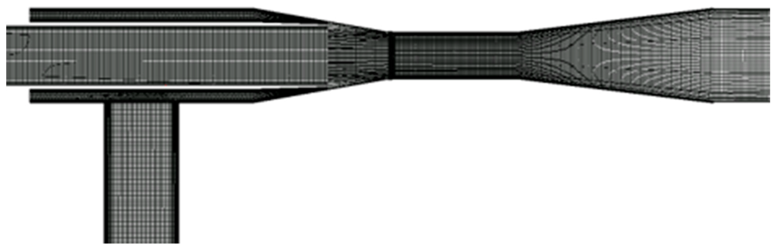
ANSYS CFX 19.2 [31] was used to perform CFD analysis, and the numerical grids were generated using ANSYS ICEM 19.2 [31]. The flow in the AJP model is steady and incompressible because it does not have any moving parts. The structured grids of the primary inlet, secondary inlet, nozzle, and diffuser of the AJP model were used for the proper CFD analysis. Figure 6 shows hexahedral grids of the inlet pipes, nozzle, and diffuser of the AJP model. The volute and the impeller structured mesh of the SCP model are shown in Figure 7. The y+ value near the wall of the primary inlet, secondary inlet, nozzle, diffuser, and outlet pipe of the AJP model are 3.54, 0.33, 2.75, 0.73, and 0.14, respectively. However, the impeller of the SCP model is a complex structure compared to the AJP model. The y+ value near the impeller wall of the SCP model is 60.
The Reynolds-averaged Navier–Stokes (RANS) equations were used to compute the steady-state analysis in AJP and SCP models. The root mean square residuals of the RANS equation for mass and momentum is maintained as lower than 10−5. The realizable κ-ε and shear stress turbulence models were selected to simulate the flow behavior in the AJP and SCP models, respectively. The realizable κ-ε turbulence model was used to evaluate the flow prediction for the spreading of jets. The realizable κ-ε model could calculate the viscous sub-layer near the wall for y+ ≤ 5 [28]. Therefore, the numerical grids for the AJP model components have a y+ value of less than 5. The shear stress transport (SST) model was adopted to conduct the CFD analysis in the SCP model. The SST model was designed to predict accurate flow using automatic near-wall treatment. The 1 < y+ < 100 range grids were suitable for the SST model with automatic near-wall treatment. The SST model was appropriate for the flow prediction in high rotation speed and strong separate flow. Hence, the y+ value for the SCP model is less than 100, which is desirable for the SST model application.
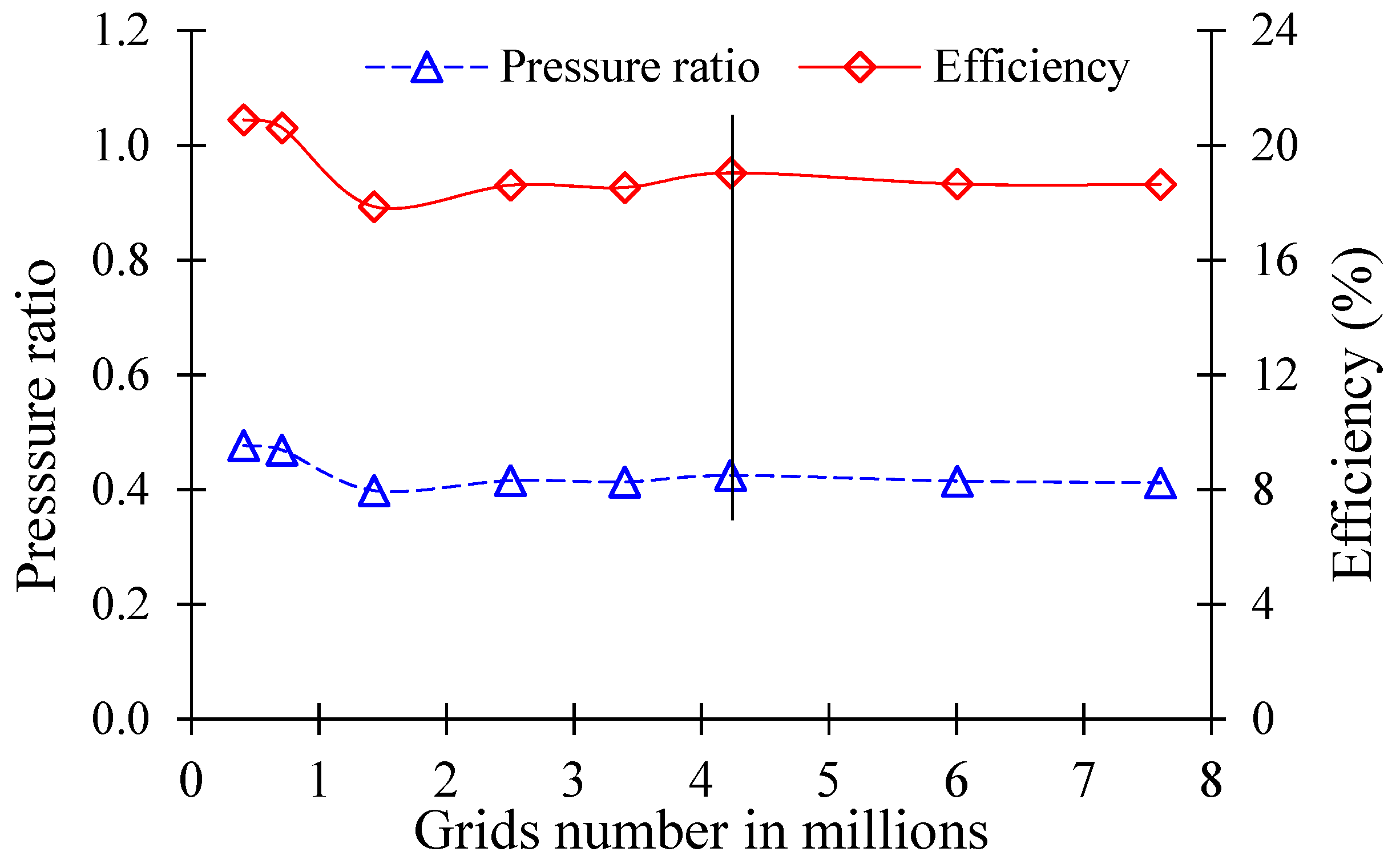
The mesh dependency test was conducted to select the optimum mesh number for the stable CFD analysis using the grid convergence index (GCI) test [32]. Table 4 and Figure 8 show the mesh dependency test results for the AJP model. The mesh dependency test concluded that 4.2 million nodes for AJP models were selected because the grid convergence index is less than 5% with stable CFD analysis results. The grid dependency test for the SCP model is shown in Table 5 and Figure 9. The deviation in the efficiency is negligible with an increase in the grid numbers. The convergence index is less than 1% for the CFD analysis of the SCP model. The mesh dependency test indicated 3.6 million nodes for the stable CFD analysis of the SCP model.
The pump efficiency, mass ratio, pressure ratio, and cavitation number were used as performance measurements for the AJP model, which was evaluated using Equations (8)–(11). Equations (12) and (13) were used to calculate the pump efficiency and cavitation number for the SCP model, respectively.
where is the mass ratio, is the pressure ratio, is the AJP model hydraulic efficiency, is the secondary flow rate, is the flow rate at the nozzle exit, is the total pressure at the diffuser outlet, is the total pressure at the secondary inlet, is the total pressure at the nozzle exit, is the cavitation number for AJP, is the static pressure at the nozzle exit, is the vapor pressure of water at 25 °C, is the velocity at the nozzle exit, is the density of water at 25 °C, is the SCP model’s hydraulic efficiency, is input torque, is the angular velocity of the impeller, is acceleration due to gravity, is flow rate, is the total head of the SCP, is the static pressure at the SCP inlet, and is the cavitation number for the SCP.
The boundary conditions for the CFD analysis for the AJP and SCP models are shown in Table 6. The inlet boundary conditions were total pressure at the primary inlet and mass flow rate at the secondary inlet of the AJP model. The outlet of the AJP was set as static pressure. The inlet and outlet of the SCP model were mass flow rate and static pressure, respectively. The mass flow rate varied from partial to full load conditions to prepare the performance curves of the SCP model. The suction performance was evaluated using the Rayleigh–Plesset equation [33].
3. Results and Discussion
3.1. Pump Performance Curves of AJP and SCP Models
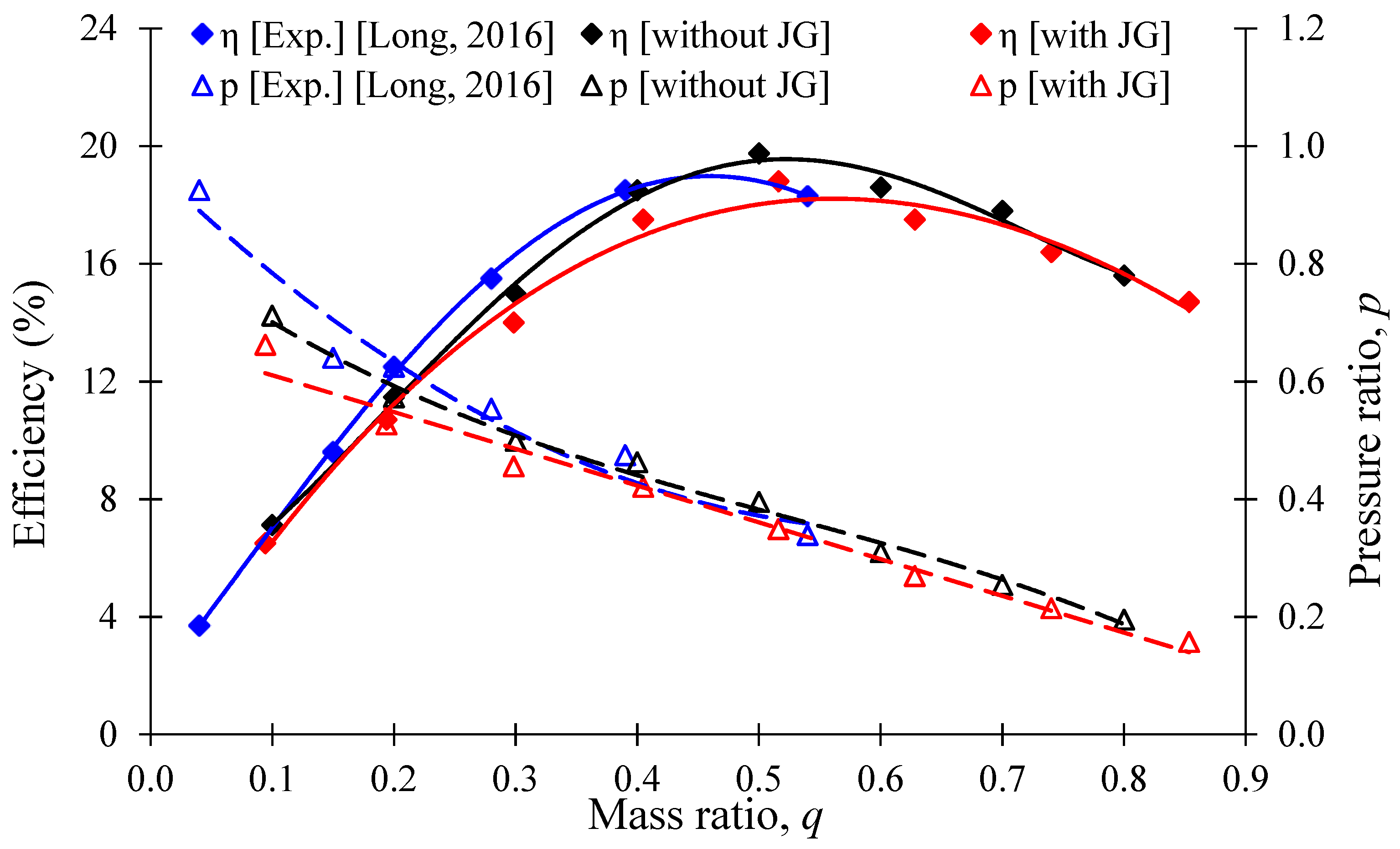
Figure 10 shows the performance curves of the AJP model. The experimental results for the AJP model were adopted from Long et al. [23]. The performance curves for the AJP model were evaluated by varying the mass ratio (q) from 0.1 to 0.8, the best efficiency point at q = 0.5. The efficiency difference between experimental data and CFD analysis results is less than 1% at q = 0.5. Hence, the experimental and CFD analysis showed good agreement between them. Therefore, the CFD analysis method is acceptable for further analysis. The best efficiencies of the AJP model without and with initial J-Groove are 19.75% and 18.88%, respectively. The installation of the J-Groove has no significant effect on the efficiency drop. It is concluded that the installation of J-Groove shows no adverse influence on the pump performance.
Figure 11 shows the performance curves for the SCP model. The best efficiency point for the SCP model matches the design point. It is concluded that the design method of the SCP model is acceptable. The best efficiencies of the SCP model are 76.54% and 71.42% without and with initial J-Groove, respectively. This showed that the installation of J-Groove has a slightly negative effect on the SCP model performance.
3.2. Suction Performance Curves of AJP and SCP Models
J-Groove installation improved the pressure distribution in the AJP and SCP models. The pressure distribution in the AJP model at = 0.4, 0.5, and 0.6 is shown in Figure 12. The minimum pressures at the throat of the AJP model without J-Groove are 82 kPa, 62 kPa, and 44 kPa at = 0.4, 0.5, and 0.6, respectively. The J-Groove passage transfers the high-pressure fluid from the diffuser to the throat and reduces the pressure at the diffuser outlet. The J-Groove installation in the AJP model increases the minimum pressure at the throat by 22%, 23%, and 40% at = 0.4, 0.5, and 0.6, respectively. The pressure improvement plays a vital role in cavitation suppression in the AJP model. Hence, the possibility of cavitation in the AJP model is reduced significantly.
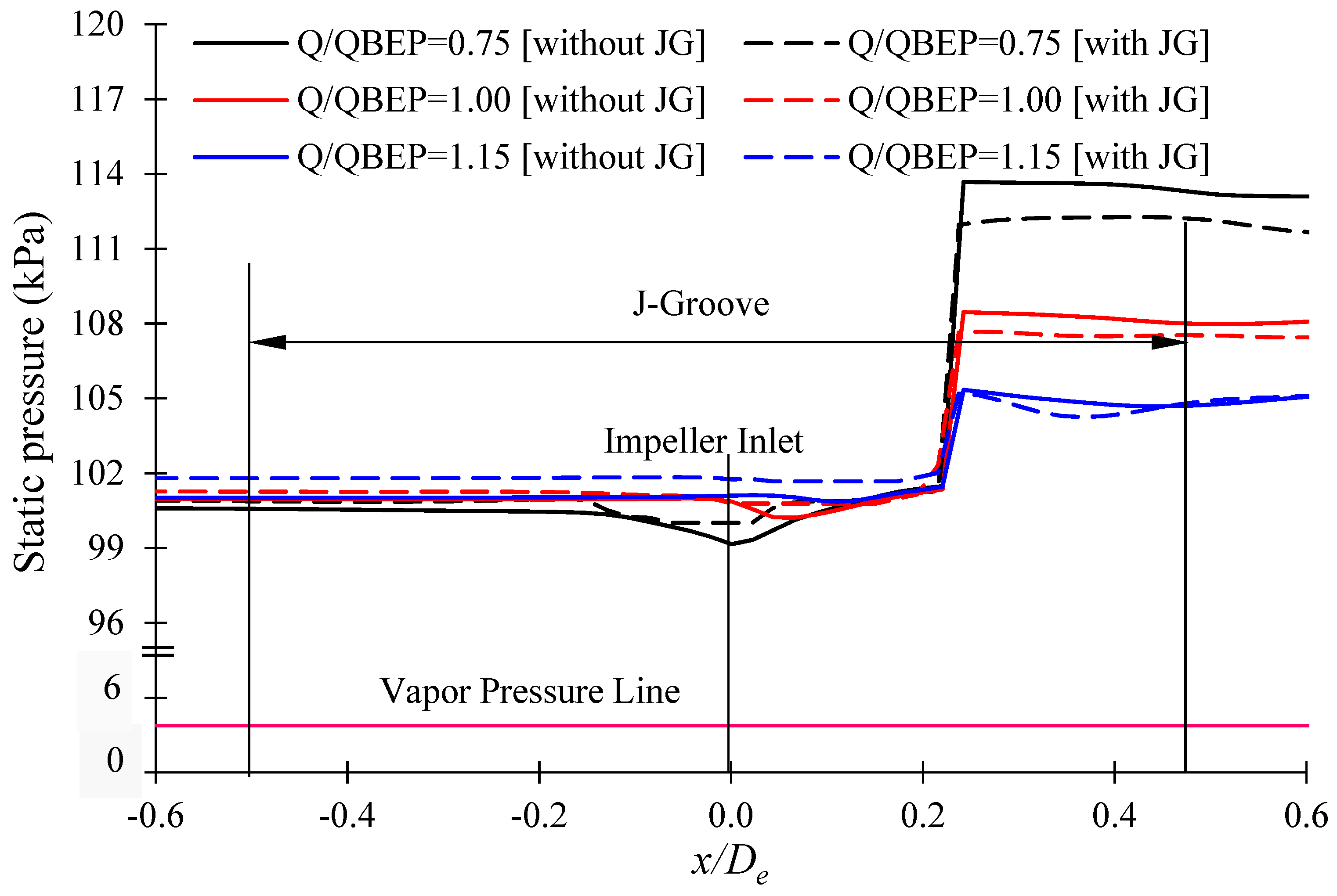
Figure 13 shows the pressure distribution in the SCP model. At the inlet of the impeller, the pressure is relatively lower than in other locations. The installation of J-Groove improves the pressure distribution at the impeller inlet in the SCP model by transferring high-pressure fluid from the impeller outlet to the impeller inlet. At = 0, the static pressure is improved in the SCP model with J-Groove. The J-Groove installation in the SCP model increases the minimum pressure at the impeller inlet by 1.1%, 1.4%, and 1.9% at Q/QBEP = 0.75, 1.00, and 1.15, respectively. It is conjectured that the reverse flow from the J-Groove passage increases the pressure at the impeller inlet and decreases the possibility of cavitation in the SCP model.
The suction performance of the AJP model without and with initial J-Groove is shown in Figure 14. The suction performance is directly affected by the pressure distribution. The critical cavitation numbers are 0.19, 0.30 and 0.38 at = 0.4, 0.5 and 0.6, respectively. The installation of J-Groove improves the suction performance in the AJP model. The critical cavitation number is improved from 0.38 to 0.30, 0.30 to 0.24 and 0.19 to 0.18 at = 0.6, 0.5 and 0.4, respectively. Hence, the installation of J-Groove drastically improves the suction performance of the AJP model.
The suction performance of the SCP model without and with initial J-Groove is shown in Figure 15. The installation of J-Groove in the SCP model is an effective method to improve the suction performance. The critical cavitation number is improved from 0.08 to 0.05 and 0.12 to 0.09 at = 0.75 and 1.00, respectively. Furthermore, the significant improvement at = 1.15 is indicated in Figure 15. The critical cavitation number is improved from 0.36 to 0.18 at < 1.15. Hence, the suction of the SCP model is improved considerably with the installation of J-Groove.
3.3. Estimation of Reverse Flow Rate by J-Groove Installation
The working mechanism of J-Groove is transferring the jet flow from the high-pressure region to the low-pressure region via groove passage [27]. The jet flow helps to increase the pressure in the low-pressure region. The reverse jet flow is dependent on the pressure difference. The reverse flow rate ratio is the mass flow rate transfer from the J-Groove passage to the best efficiency flow rate for the AJP and SCP models, respectively. The reverse flow rate ratio is used to evaluate the flow mechanism in the J-Groove. The reverse flow rate ratio is calculated using Equation (12).
Where is the reverse flow rate ratio, is the reverse mass flow rate through J-Groove (kg/s), and is the mass flow rate of AJP or SCP model at the BEP.
The reverse flow rate ratio and pressure difference variation in the J-Groove passage of AJP and SCP is shown in Figure 16, and d represents the size ratio of J-Groove depth. In the AJP model, the reverse flow rate ratio increases with an increase in the flow rate. However, in the SCP model, the reverse flow rate ratio decreases with an increase in the flow rate. The variation in reverse flow rate ratio and pressure difference with J-Groove depth in AJP and SCP models is shown in Figure 16. The variation in pressure distribution causes the difference in the reverse flow rate ratio at various flow rates. The pressure difference between the J-Groove inlet and outlet is higher in the high load condition than in the partial load condition in the AJP model. Similarly, the pressure difference is higher in the partial load condition than in the high load condition in the SCP model. Therefore, the reverse flow behavior is contradictory between the AJP and SCP models.
The pressure contours in the AJP model are shown in Figure 17. The absence of moving components is the reason for the smooth pressure distribution in the AJP model. Figure 17 shows the pressure difference between the J-Groove inlet and outlet in the AJP model. The velocity vector in the AJP model with J-Groove is shown in Figure 18. The velocity vector in the J-Groove passage is in the opposite direction to the main flow. The velocity vectors show that the installation of J-Groove improves the pressure distribution by reverse jet flow. It is concluded that the J-Groove induces the reverse jet flow, which improves suction performance.
The pressure contours in the SCP model are shown in Figure 19. The pressure is increased considerably via the impeller. A clear difference in the pressure distribution is observed in the SCP model. The rotation of the impeller increases the pressure drastically in the SCP model. Figure 20 shows the velocity vectors in the SCP model with J-Groove. The velocity vector clarifies the reverse jet flow occurrence in the J-Groove flow passage, the direction of which is opposite to the main flow. The pressure difference between the J-Groove inlet and outlet induces the reverse flow in the AJP and SCP models.
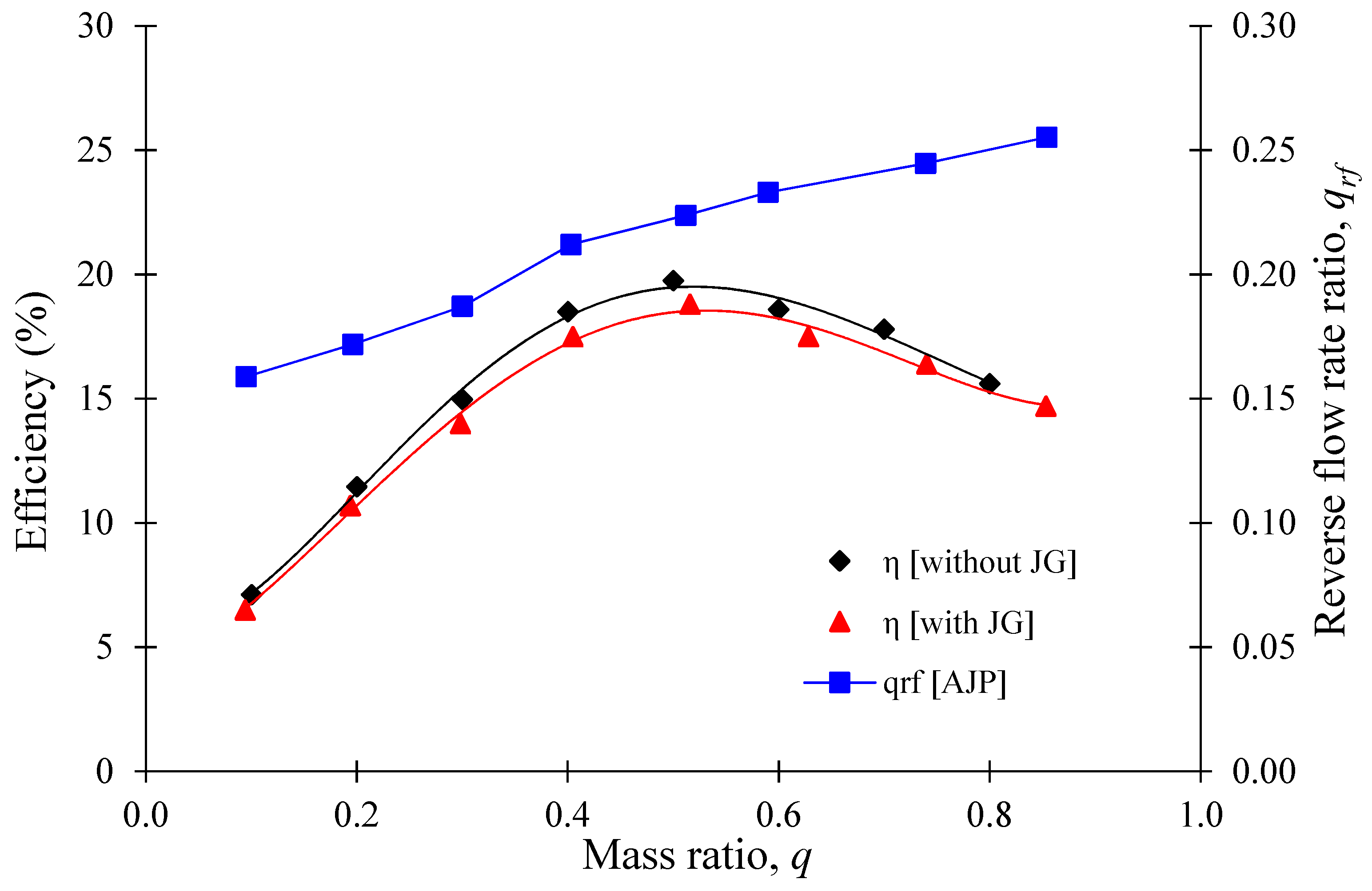
3.4. Relationship between Reverse Flow Rate in J-Groove Channel and Pump Performance
The comparison of the performance curves and reverse flow rate ratio in the AJP model is shown in Figure 21. The reverse flow rate ratio varies from 0.16 to 0.26 in the AJP model. The pump efficiency decreases with an increase in the reverse flow rate ratio. When the reverse flow rate ratio is 0.16 and 0.25, the efficiency is reduced by 0.61% and 0.93%, respectively. The efficiency drop in the AJP model is below 1%, which is insignificant. Figure 22 shows the relation between the reverse flow rate ratio and efficiency drop in the SCP model. In the SCP model, the reverse flow rate ratio is comparatively lower than the AJP model because the design flow rate for the SCP model is higher than the AJP model. When = 0.064 and 0.014, the efficiency drops by 2.97% and 1.58% in the SCP model, respectively. The reverse flow rate ratio has a higher efficiency drop in the SCP model than in the AJP model. Hence, the reverse flow rate ratio increases the static pressure at the expense of efficiency drop.
3.5. Relationship between Reverse Flow Rate in J-Groove Channel and Suction Performance
The suction performance and reverse flow rate ratio in the AJP model are shown in Figure 23. The reverse jet flow is dependent on the mass ratio and cavitation number. The reverse flow rate ratio increases with an increase in mass ratio. The reverse flow rate ratio is reduced drastically at the critical cavitation number. When the critical cavitation number is reached, the cavitation clouds are formed at the throat and diffuser of the AJP model and obstruct the reverse flow. At = 0.36, the reverse flow rate ratios are 0.14, 0.16, and 0.17 for = 0.4, 0.5, and 0.6, respectively. The reverse flow rate ratio indicates the occurrence of a critical cavitation number. Figure 23 shows the gradual decrease in the reverse flow rate ratio when the cavitation number () approaches the critical value. The reverse flow rate ratio plays an important role in cavitation prediction in the AJP model.
Figure 24 shows the relation between suction performance and reverse flow rate ratio in the SCP model. The reverse flow rate ratio decreases with an increase in flow rate. At = 0.5, the reverse flow rate ratios are 0.09, 0.03, and 0.01 for = 0.75 and 1.00 and 1.15, respectively. The reverse flow rate ratio decreases drastically with an increase in flow rate in the SCP model. The reverse flow rate ratio tends to decrease gradually when the cavitation number approaches the critical cavitation number. This indicates that the cavitation will initiate with a gradual decrease in the reverse flow rate ratio. The cavitation possibility increases with a decrease in the reverse flow rate ratio in the AJP and SCP models. Figure 23 and Figure 24 confirm that the reverse flow rate ratio tendency with cavitation number is similar in the AJP and SCP models. The reverse flow rate ratio () can predict the cavitation inception and avoid severe damage to the AJP and SCP models.
3.6. Mechanism of Reverse Flow Rate in AJP and SCP Models
The J-Groove installation induces the reverse flow in the AJP and SCP models. In the AJP model, the fluid flows from the inlet to the outlet via the venturi effect [34]. The continuous primary flow passes through the throat at high velocity from the booster pump. The air is removed from the nozzle, creating a vacuum, and secondary flow is sucked up due to the atmospheric pressure. Finally, the secondary flow is mixed with the high-velocity primary flow at the throat, and the mixed flow passes through a diffuser which gradually reduces the velocity. The J-Groove installation creates the simple narrow flow passages in the wall of the AJP model. The flow behavior in the J-Groove is dependent on the pressure difference. CFD analysis indicated that the pressure at the J-Groove outlet is higher than the J-Groove inlet, which is in the reverse direction to the main flow. Figure 25 elaborates the flow mechanism of the J-Groove in the AJP model.
In the SCP, the flow behavior is like an inducer. The impeller rotation transfers flow from a low-pressure inlet to a high-pressure outlet. The installation of J-Groove in the SCP induces reverse flow through the groove channels due to the pressure difference. Therefore, the J-Groove passage transfers flow from the outlet to the inlet of the diffuser casing. The J-Groove flow mechanism in the SCP model is shown in Figure 26.
4. Conclusions
The CFD analysis showed that the J-Groove installation in the AJP and SCP models improves the suction performance. The pressure distribution and suction performance of AJP and SCP models are improved drastically with J-Groove installation. The reverse flow rate plays a significant role in suction performance improvement. The pressure distribution in the AJP and SCP models is different because of the impeller. In the AJP model, the reverse flow rate ratio increases with an increase in flow rate. However, the reverse flow rate ratio decreases with an increase in flow rate in the SCP model. The installation of the impeller has a significant impact on the reverse flow rate in the diffuser. In the AJP model, the pressure difference between the inlet and outlet of J-Groove is higher in full load conditions than in partial load conditions. The reverse flow rate is dependent on the pressure difference. In the SCP model, the pressure difference is larger at partial load conditions compared to full load conditions.
The suction performance is directly related to the reverse flow rate ratio. The study concluded that the reverse flow rate ratio is dependent on the pump type, flow rate, and cavitation number. The higher reverse flow rate ratio improves the suction performance in the AJP and SCP models effectively. The reverse flow mechanism in the AJP and SCP models is different. In the AJP model, the simple pressure difference between the inlet and outlet of J-Groove induces the reverse flow. In the SCP model, the rotation of the impeller causes a pressure difference between the suction and pressure side, which contributes to the reverse flow. It is concluded that the J-Groove installation helps to increase the reverse flow rate mainly due to the pressure difference.
Author Contributions
Conceptualization, U.S. and Y.-D.C.; methodology, U.S.; software, Y.-D.C.; validation, U.S. and Y.-D.C.; formal analysis, U.S.; investigation, U.S.; resources, Y.-D.C.; data curation, U.S.; writing—original draft preparation, U.S.; writing—review and editing, U.S. and Y.-D.C.; visualization, U.S.; supervision, Y.-D.C.; project administration, Y.-D.C.; funding acquisition, Y.-D.C. All authors have read and agreed to the published version of the manuscript.
Funding
This research received no external funding.
Conflicts of Interest
The authors declare no conflict of interest.
References
- Elger, D.F.; Mclam, E.T.; Taylor, S.J. A new way to represent jet pump performance. J. Fluids Eng. 1991, 113, 439–444. [Google Scholar] [CrossRef]
- Deng, X.; Dong, J.; Wang, Z.; Tu, J. Numerical analysis of an annular water-air jet pump with self-induced oscillation mixing chamber. J. Comput. Multiph. Flows 2017, 9, 47–53. [Google Scholar] [CrossRef]
- Kryzhanivskyi, Y.I. The study on the flow’s kinematics in the jet pump’s mixing chamber. Geotech. Min. Mech. Eng. Mach. Build. 2019, 1, 62–68. [Google Scholar]
- Kim, Y.K.; Lee, D.Y.; Kim, H.D.; Ahn, J.H.; Kim, K.C. An experimental and numerical study on hydrodynamic characteristics of horizontal annular type water-air ejector. J. Mech. Sci. Technol. 2012, 26, 2773–2781. [Google Scholar] [CrossRef]
- Nilavalagan, S.; Ravindran, M.; RadhaKrishna, H.C. Analysis of mixing characteristics of flow in a jet pump using a finite-difference method. Chem. Eng. J. 1988, 39, 97–109. [Google Scholar] [CrossRef]
- Elger, D.F.; Taylor, S.J.; Liou, C.P. Recirculation in an annular-type jet pump. J. Fluids Eng. 1994, 116, 735–740. [Google Scholar] [CrossRef]
- Hatzlavramidls, D.T. Modeling and design of jet pumps. SPE Prod. Eng. 1991, 6, 413–419. [Google Scholar] [CrossRef]
- Narabayashi, T.; Yamazaki, Y.; Kobayashi, H.; Shakouchi, T. Flow analysis for single and multi-nozzle jet pump. JMSE Int. J. 2006, 49, 933–940. [Google Scholar] [CrossRef] [Green Version]
- Zhu, H.; Qiu, B.; Jia, Q.; Yang, X. Simulation analysis of hydraulic jet pump. Adv. Mater. Res. 2011, 204, 293–296. [Google Scholar] [CrossRef]
- Shimizu, Y.; Nakamura, S.; Kuzuhara, S.; Kurata, S. Studies of the configuration and performance of annular type jet pumps. J. Fluids Eng. 1987, 190, 205–212. [Google Scholar] [CrossRef]
- Hammoud, A.H. Effect of design and operational parameters on jet pump performance. In Proceedings of the 4th WSEAS International Conference on Fluid Mechanics and Aerodynamics, Elounda, Greece, 21 August 2006. [Google Scholar]
- Kwon, O.B.; Kim, M.K.; Kwon, H.C.; Bae, D.S. Two-dimensional numerical simulations on the performance of an annular jet pump. J. Vis. 2002, 5, 21–28. [Google Scholar] [CrossRef]
- Song, X.G.; Park, J.H.; Kim, S.G.; Park, Y.C. Performance comparison and erosion prediction of jet pumps by using a numerical method. Math. Comput. Model. 2013, 57, 245–253. [Google Scholar] [CrossRef]
- Guan, X.F. Modern Pump Theory and Design; China Astronaut: Beijing, China, 2011. (In Chinese) [Google Scholar]
- Kim, Y.; Tanaka, K.; Lee, Y.; Matsumoto, Y. Effects of entrained air on the characteristics of a small screw-type centrifugal pump. KSFM J. Fluid Mach. 2011, 2, 37–44. [Google Scholar]
- Tatebayashi, Y.; Tanaka, K. Influence of meridional shape on screw-type centrifugal pump performance. In Proceedings of the ASME Fluids Engineering Division Summer Meeting, FEDSM2002-31183, Montreal, QC, Canada, 14–18 July 2002; pp. 769–776. [Google Scholar]
- Tatebayashi, Y.; Tanaka, K.; Kobayashi, T. Thrust prediction in screw-type centrifugal pump. In Proceedings of the 4th ASME_JSME Joint Fluid Engineering Conference, FEDSM2003-45105, Honolulu, HI, USA, 6–10 July 2003; pp. 621–626. [Google Scholar]
- Cheng, X.; Lia, R. Parameter equation study for screw centrifugal pump. Procedia Eng. 2012, 31, 914–921. [Google Scholar] [CrossRef] [Green Version]
- Guo, M.; Choi, Y.-D. Design and CFD analysis of a screw centrifugal pump model. J. Korean Soc. Mar. Eng. 2017, 43, 640–647. [Google Scholar] [CrossRef]
- Franc, J.P. Partial cavity instabilities and re-entrant jet. In Proceedings of the 4th International Symposium on Cavitation, Grenoble, France; 2001. [Google Scholar]
- Xiao, L.; Long, X. Cavitating flow in annular jet pumps. Int. J. Multiph. Flow 2015, 71, 116–132. [Google Scholar] [CrossRef]
- Cunningham, R.G.; Hansen, A.G.; Na, T.Y. Jet Pump Cavitation. J. Basic Eng. 1970, 92, 483–492. [Google Scholar] [CrossRef]
- Long, X.; Xu, M.; Lyu, Q.; Zou, J. Impact of the internal flow in a jet fish pump on the fish. Ocean Eng. 2016, 126, 313–320. [Google Scholar] [CrossRef]
- Cochran, D.L.; Kline, S.J. Use of Short Flat Vanes for Producing Efficient Wide-Angle Two-dimensional Diffusers. NASA Tech. Note 1958, 4309, 1–130. [Google Scholar]
- Kurokawa, J.; Imamura, H.; Choi, Y.-D. Effect of J-groove on the suppression of swirl flow in a conical diffuser. J. Fluids Eng. 2010, 132, 071101. [Google Scholar] [CrossRef]
- Choi, Y.-D.; Kurokawa, J.; Imamura, H. Suppression of cavitation in inducers by J-Grooves. J. Fluids Eng. 2007, 129, 15–22. [Google Scholar] [CrossRef]
- Choi, Y.-D.; Shrestha, U. Cavitation performance improvement of an annular jet pump by J-groove. KSFM J. Fluid Mach. 2020, 26, 25–35. [Google Scholar] [CrossRef]
- Shrestha, U.; Choi, Y.-D. Effect of diffuser angle and J-groove depth on improvement in suction performance of annular jet pump model. J. Adv. Mar. Eng. Technol. 2020, 44, 385–394. [Google Scholar] [CrossRef]
- Shrestha, U.; Choi, Y.-D. Suction performance improvement of an annular jet pump by J-Groove passage shape optimization. J. Mech. Sci. Technol. 2021, 35, 5517–5527. [Google Scholar] [CrossRef]
- Hoang, T.H.M.; Truong, V.A.; Shrestha, U.; Choi, Y. Optimization of the Meridional Plane Shape Design Parameters in a Screw Centrifugal Pump Impeller. KSFM J. Fluid Mach. 2021, 24, 15–25. [Google Scholar] [CrossRef]
- ANSYS. ANSYS CFX Documentation; ANSYS Inc.: Canonsburg, PA, USA, 2017. [Google Scholar]
- Celik, I.B.; Ghia, U.; Roache, P.J.; Freitas, C.J. Procedure for estimation and reporting of uncertainty due to discretization in CFD applications. J. Fluids Eng.-Trans. ASME 2008, 130, 078001. [Google Scholar]
- Franc, J. The Rayleigh-Plesset equation: A simple and powerful tool to understand various aspects of cavitation. In Fluid Dynamics of Cavitation and Cavitating Turbopumps; Springer: Berlin/Heidelberg, Germany, 2007; pp. 1–41. [Google Scholar]
- Xu, K.; Wang, G.; Wang, L.; Yun, F.; Sun, W.; Wang, X.; Chen, X. CFD-Based Study of Nozzle Section Geometry Effects on the Performance of an Annular Multi-Nozzle Jet Pump. Processes 2020, 8, 133. [Google Scholar] [CrossRef] [Green Version]
Figure 1.
Workflow process for the estimation of reverse flow in AJP and SCP models with J-Groove.

Figure 2.
Three-dimensional and schematic views of annular jet pump (AJP) model.

Figure 3.
(a) Three-dimensional view and (b) meridional shape of screw centrifugal pump (SCP) model.
Figure 3.
(a) Three-dimensional view and (b) meridional shape of screw centrifugal pump (SCP) model.

Figure 4.
Schematic view of J-Groove shape parameters in annular jet pump model.

Figure 5.
Schematic view of J-Groove shape parameters in screw centrifugal pump model.

Figure 6.
Numerical grids of annular jet pump model.

Figure 7.
Numerical grids of (a) impeller of SCP, (b) volute, and (c) cross-section view of impeller with J-Groove.
Figure 7.
Numerical grids of (a) impeller of SCP, (b) volute, and (c) cross-section view of impeller with J-Groove.

Figure 8.
Grid dependency test for AJP model.

Figure 9.
Grid dependency test for SCP model.

Figure 10.
Comparison of performance curves between experimental [23] and CFD analysis of AJP model without and with J-Groove (JG).
Figure 10.
Comparison of performance curves between experimental [23] and CFD analysis of AJP model without and with J-Groove (JG).

Figure 11.
Performance curves comparison without and with J-Groove in SCP model.

Figure 12.
Pressure distribution comparison in the AJP model without and with J-Groove.

Figure 13.
Pressure distribution comparison in the SCP model without and with J-Groove.

Figure 14.
Suction performance comparison in the AJP model without and with J-Groove.

Figure 15.
Suction performance comparison in the SCP model without and with J-Groove.

Figure 16.
Reverse flow rate ratio and pressure difference variation in the J-Groove channel of AJP and SCP models.
Figure 16.
Reverse flow rate ratio and pressure difference variation in the J-Groove channel of AJP and SCP models.

Figure 17.
Pressure contours in the AJP model with J-Groove at q = 0.5.

Figure 18.
Velocity vectors in the AJP model with J-Groove at q = 0.5.

Figure 19.
Pressure contours in the SCP model with J-Groove at Q/QBEP = 1.00.

Figure 20.
Velocity vector distribution in the SCP model with J-Groove at Q/QBEP = 1.00.

Figure 21.
Performance curves of AJP model with reverse flow rate ratio.

Figure 22.
Performance curves of SCP model with reverse flow ratio.

Figure 23.
Relationship between suction performance and reverse flow rate in the AJP model with J-Groove.
Figure 23.
Relationship between suction performance and reverse flow rate in the AJP model with J-Groove.

Figure 24.
Relationship between suction performance and reverse flow rate ratio in the SCP model with J-Groove.
Figure 24.
Relationship between suction performance and reverse flow rate ratio in the SCP model with J-Groove.

Figure 25.
Mechanism of reverse flow in AJP model with J-Groove.

Figure 26.
Mechanism of reverse flow in SCP model with J-Groove.


Table 1.
Specification of annular jet pump model [29].
Table 1.
Specification of annular jet pump model [29].
| Nomenclature | Size Ratio | Values |
|---|---|---|
| 2.08 | ||
| 1.67 | ||
| 1.33 | ||
| 1.53 | ||
| 1.00 | ||
| 8.33 | ||
| 2.7 | ||
| 3.5° | ||
| 20.0° | ||
| 1.75 |
Table 2.
Specification of screw centrifugal pump model [30].
Table 2.
Specification of screw centrifugal pump model [30].
| Nomenclature | Size Ratio | Value |
|---|---|---|
| 1.39 | ||
| 1.30 | ||
| 1.00 | ||
| 0.46 | ||
| 1.46 | ||
| 1.09 | ||
| 0.61 | ||
| 0.35 | ||
| 0.13 | ||
| 0.30 | ||
| 30.0° | ||
| 41.2° | ||
| 39.9° | ||
| 10.0° |
Table 3.
Shape parameters of J-Groove for AJP and SCP models.
| Nomenclature | J-Groove in AJP Model | J-Groove in SCP Model | ||
|---|---|---|---|---|
| Size Ratio | Value | Size Ratio | Value | |
| 0.06 | 0.01 | |||
| 0.32 | 0.44 | |||
| 12° | 12° | |||
| 15 | 15 | |||
Table 4.
Grid dependency test for AJP CFD analysis via GCI method.
| 2.1766 | 2.1766 | 2.1766 | |
| 2.6461 | 2.6461 | 2.6461 | |
| 0.4486 | 0.3981 | 17.8600 | |
| 0.4484 | 0.4246 | 19.0400 | |
| 0.24 | 0.4118 | 18.6300 | |
| 0.0040 | −0.0128 | −0.4100 | |
| −0.0002 | 0.0265 | 1.1800 | |
| 0.8352 | 1.3240 | 1.4327 | |
| 0.4488 | 0.3880 | 17.4707 | |
| 0.847% | 3.441% | 4.311% | |
| 0.798% | 7.413% | 7.790% | |
| 0.044% | 3.168% | 2.724% |
where is the refinement factor between the coarse and fine grid, is the mass ratio, is the pressure ratio, is efficiency, is the formal order of accuracy of the algorithm, , , is the approximate relative error, is the extrapolated relative error, and is the fine-grid convergence index.
Table 5.
Grid dependency test for SCP CFD analysis via GCI method.
| 1.095 | 1.095 | 1.095 | |
| 1.110 | 1.110 | 1.110 | |
| 73.414 | 2.912 | 2.478 | |
| 73.469 | 2.917 | 2.471 | |
| 72.879 | 2.876 | 2.466 | |
| −0.589 | −0.041 | −0.015 | |
| 0.055 | 0.005 | 0.003 | |
| 23.016 | 20.941 | 15.305 | |
| 73.489 | 2.919 | 2.482 | |
| 0.075% | 0.163% | 0.128% | |
| 0.102% | 0.217% | 0.159% | |
| 0.013% | 0.036% | 0.053% |
where is the refinement factor between the coarse and fine grid, is the efficiency, is power (kW), and is head (m).
Table 6.
Information of boundary conditions for CFD analysis of AJP and SCP models.
| Parameter/Boundary | Condition/Value | |
|---|---|---|
| AJP | SCP | |
| Primary Inlet | Total Pressure | Mass Flow Rate |
| Secondary Inlet | Mass Flow Rate | - |
| Outlet | Static Pressure | Static Pressure |
| Turbulence model | Realizable κ-ε | SST |
| Grid interface connection | General Grid Interface (GGI) | General Grid Interface (GGI) |
| Interface model | Steady State/Frozen rotor | Steady State/Frozen rotor |
| Walls | No slip wall (roughness: smooth) | No slip wall (roughness: smooth) |
Publisher’s Note: MDPI stays neutral with regard to jurisdictional claims in published maps and institutional affiliations. |
© 2022 by the authors. Licensee MDPI, Basel, Switzerland. This article is an open access article distributed under the terms and conditions of the Creative Commons Attribution (CC BY) license (https://creativecommons.org/licenses/by/4.0/).
Share and Cite
MDPI and ACS Style
Shrestha, U.; Choi, Y.-D. Estimation of Reverse Flow Rate in J-Groove Channel of AJP and SCP Models Using CFD Analysis. Processes 2022, 10, 785. https://0-doi-org.brum.beds.ac.uk/10.3390/pr10040785
AMA Style
Shrestha U, Choi Y-D. Estimation of Reverse Flow Rate in J-Groove Channel of AJP and SCP Models Using CFD Analysis. Processes. 2022; 10(4):785. https://0-doi-org.brum.beds.ac.uk/10.3390/pr10040785
Chicago/Turabian StyleShrestha, Ujjwal, and Young-Do Choi. 2022. "Estimation of Reverse Flow Rate in J-Groove Channel of AJP and SCP Models Using CFD Analysis" Processes 10, no. 4: 785. https://0-doi-org.brum.beds.ac.uk/10.3390/pr10040785
Note that from the first issue of 2016, this journal uses article numbers instead of page numbers. See further details here.