Multilayer Reversible Data Hiding Based on the Difference Expansion Method Using Multilevel Thresholding of Host Images Based on the Slime Mould Algorithm

Abstract

Researchers have scrutinized data hiding schemes in recent years. Data hiding in standard images works well, but does not provide satisfactory results in distortion-sensitive medical, military, or forensic images. This is because placing data in an image can cause permanent distortion after data mining. Therefore, a reversible data hiding (RDH) technique is required. One of the well-known designs of RDH is the difference expansion (DE) method. In the DE-based RDH method, finding spaces that create less distortion in the marked image is a significant challenge, and has a high insertion capacity. Therefore, the smaller the difference between the selected pixels and the more correlation between two consecutive pixels, the less distortion can be achieved in the image after embedding the secret data. This paper proposes a multilayer RDH method using the multilevel thresholding technique to reduce the difference value in pixels and increase the visual quality and the embedding capacity. Optimization algorithms are one of the most popular methods for solving NP-hard problems. The slime mould algorithm (SMA) gives good results in finding the best solutions to optimization problems. In the proposed method, the SMA is applied to the host image for optimal multilevel thresholding of the image pixels. Moreover, the image pixels in different and more similar areas of the image are located next to one another in a group and classified using the specified thresholds. As a result, the embedding capacity in each class can increase by reducing the value of the difference between two consecutive pixels, and the distortion of the marked image can decrease after inserting the personal data using the DE method. Experimental results show that the proposed method is better than comparable methods regarding the degree of distortion, quality of the marked image, and insertion capacity.

1. Introduction

Data hiding (DH) is a way of secretly sending information or data to others. In this way, data, including text, images, etc., can be inserted into a medium such as an image, video, audio, etc., using a DH algorithm to make them invisible to others. DH is performed in two domains of space and frequency. The related data are inserted directly into the host image pixels in the space domain, which is often reversible. Reversibility means that the inserted data and the original host image are entirely recovered in the extraction phase. In the frequency domain, first, a frequency transform such as discrete wavelet transform (DWT), discrete cosine transform (DCT), etc., is applied to the host image. Then, using a special algorithm, the data are inserted into frequency coefficients that are often irreversible. The data are then extracted, while the original host image is not fully and accurately recovered.

Reversible data hiding (RDH) techniques in the space field are divided into several categories: difference expansion (DE), histogram shifting (HS), prediction-error expansion (PEE), pixel value grouping (PVG), and pixel value ordering (PVO). Over the years, various RDH methods have been proposed by researchers in these fields, all of which aim to reduce distortion and increase the quality of the marked image or increase the capacity to insert the data, and these issues continue. As the main challenge, this has occupied the minds of researchers. The following is a brief description of the papers available in each field:

An RDH method was proposed in [1] to increase the capacity based on the DE method. In this method, the host image is divided into 1 × 2 blocks, and spaces of −1, 0, and +1 are selected to insert the data. A lossless RDH method based on the DE histogram (DEH) was proposed to increase the capacity in [2], where the difference histogram (DH) peak point was selected to insert the data. In [3], a multilayer RDH method based on the DEH was proposed to increase the capacity and reduce the distortion. However, this method was not able to improve the capacity sufficiently. In [4], the RDH method was presented for gray images using the DEH and the module function. The position matrix and the marked image were sent separately to the receiver with low capacity.

In [5], to improve the capacity performance and increase security, a guided filter predictor and an adaptive PEE design were used to insert the data in color images using intrachannel correlation. A two-layer DH method based on the expansion and displacement of a PE pair in a two-dimensional histogram was proposed to increase the capacity by extracting the correlations between the consecutive PEs in [6], where their work was both low-capacity and low-quality. In [7], the authors presented an RDH method based on the multiple histogram correction and PEE to increase the capacity of the gray images, using a rhombus predictor to predict the host image pixels. In PE histogram (PEH) methods [8], to extract the redundancy between adjacent pixels, the correction path detection strategy is used to obtain a two-dimensional PEH that has a high distortion. In an RDH method [9], based on a two-layer insertion and PEH, the pixel pairs are selected based on pixel density and the spatial distance between two pixels. The distortion is much less than in the previous methods. In [10], an RDH method based on multiple histogram shifting was proposed that used a genetic algorithm (GA) to control the substantial image distortion. In [11], an RDH technique was proposed based on pairwise prediction-error expansion (PPEE) or two-dimensional PEH (2D-PEH) to increase capacity. In [12], an RDH technique based on the host image texture analysis was proposed by blocking the image and inserting the data into image texture blocks [13,14,15,16,17,18,19,20].

In another RDH method [21], the PVG method was used by multilayer insertion to increase the capacity. The PVG was applied on each block. The zero point of the histogram of the difference was selected to insert the data bits. The pixel-based PVG (PPVG) technique in [22] was proposed to increase the capacity applied to each block after image blocking. Each time a pixel is located in the smooth areas of each block for inserting the data, the PE value is the difference between the reference pixel and the particular pixel. This method has a low capacity and moderate distortion. In [23], a technique was presented to increase the reliability of the image for inserting the data. Using PEE based on PVO, the authors inserted the data in the pins of −1 and +1 from the PEH. The problem was that the quality of the image was still low, while the capacity was not high. The authors of [24] presented a robust reversible data hiding (RRDH) scheme based on two-layer embedding with a reduced capacity-distortion tradeoff, where it first decomposes the image into two planes—namely, the higher significant bit (HSB) and least important bit (LSB) planes—and then employs prediction-error expansion (PEE) to embed the secret data into the HSB plane.

In [25], the authors proposed an AMBTC-based RDH method in which the hamming distance and PVD methods were used to insert information. In [26], a PVD-based RDH method was used. In [27], the RDH method was based on PVD and LSB reversible insert information. The authors of [28] proposed an RDH in encrypted images (RDHEI) method with hierarchical embedding based on PE. PEs are divided into three categories: small-magnitude, medium-magnitude, and large-magnitude. In their approach, pixels with small-magnitude/large-magnitude PEs were used to insert data. Their method had a high capacity, but the image quality was still low.

The authors of [29] proposed an RDH method for color images using HS-based double-layer embedding. The authors used the image interpolation method to generate PE matrices for HS in the first-layer embedding, and local pixel similarity to calculate the difference matrices for HS in the second-layer embedding. In their process, the embedding capacity was low. In [30], the authors proposed a dual-image RDH method based on PE shift. Moreover, in their work, a bidirectional-shift strategy was used to extend the shiftable positions in the central zone of the allowable coordinates. In their work, the embedding capacity was low. Today, optimization algorithms such as the grasshopper optimization algorithm (GOA), whale optimization algorithm (WOA), moth–flame optimization (MFO) [31], Harris hawk optimization (HHO) [32], and artificial bee colony (ABC) [33] are used in many papers [34,35,36,37,38].

This paper proposes a DE-based multilayer image RDH method using the multilevel thresholding technique. Optimization algorithms are one of the most popular methods for solving NP-hard problems. Due to this, the slime mould algorithm (SMA) gives good results in finding the best solutions to solve optimization problems. First, the SMA is applied to the host image to find the two thresholds, and image pixels are based on the thresholds located in three different classes. Using the multilevel thresholding creates more similarities between the pixels of each class. Therefore, due to the reduction in the difference between each class’ pixels, the quality of the marked image does not decrease with the insertion of data via DE. At the same time, less distortion is created in the picture, and the insertion capacity increases.

Table 1. Key acronyms and their meanings.

Key Acronyms	Their Meanings
DH	Data hiding
DWT	Discrete wavelet transform
DCT	Discrete cosine transform
RDH	Reversible data hiding
DE	Difference expansion
HS	Histogram shifting
PEE	Prediction-error expansion
PVG	Pixel value grouping
PVO	Pixel value ordering
DH	Difference histogram
PEH	PE histogram
GA	Genetic algorithm
PPEE	Pairwise prediction-error expansion
2D-PEH	Two-dimensional PEH
RRDH	Robust reversible data hiding
HSB	Higher significant bit
LSB	Least important bit
PEE	Prediction-error expansion
RDHEI	RDH in encrypted images
MSE	Mean squared error
PSNR	Peak signal-to-noise ratio
bpp	Bits per pixel
SSIM	Structural similarity index measure

shows the critical acronyms and their meanings.

The method of Arham et al. [3] is the basis of the proposed method. Arham et al. [3] proposed a multilayer RDH method to reduce the distortion in the image. First, the host image is divided into 2 × 2 blocks in their work. Then, to calculate the value of differences for both consecutive pixels, the pixel vector is created for each block in each layer, as shown in Figure 1. A threshold $\left(2\le \mathrm{Th}\le 30\right)$ is considered, and only the blocks in which the value of differences for both consecutive pixels is positive and less than the threshold value (2 ≤ Th ≤ 30) are selected to insert the data.

For each the vectors ${\mathrm{w}}_{\mathrm{s}}$ where $\mathrm{s}=\left\{0,1,2,3\right\}$ in the $\mathrm{s}$-th insertion layer, in order to ensure reversibility and extract the data in the extraction phase, the $\mathrm{s}$-th pixel from each block is not inserted, there is a reference pixel in each insertion layer, and three bits of data are inserted in a block of size 2 × 2. In the first insertion layer, in Figure 1, the pixel vector ${\mathrm{w}}_{\mathrm{s}}$ is created to calculate the values of ${\mathrm{v}}_1$, ${\mathrm{v}}_2$, ${\mathrm{v}}_3,$. The value of differences is calculated using Equation (1) for both consecutive pixels:

$${\mathrm{v}}_1={\mathrm{u}}_1-{\mathrm{u}}_0,{\mathrm{v}}_2={\mathrm{u}}_2-{\mathrm{u}}_1,{\mathrm{v}}_3={\mathrm{u}}_3-{\mathrm{u}}_2$$

(1)

Furthermore, to reduce the distortion and control of overflow/underflow, Equation (2) is used to reduce the value of ${\mathrm{v}}_{\mathrm{k}}$ $\left(\mathrm{k}=1,2,3\right)$:

$${\mathrm{v}}_{\mathrm{k}}^{\prime }=\{\begin{array}{c}{\mathrm{v}}_{\mathrm{k}}-2^{\left|{\mathrm{v}}_{\mathrm{k}}\right|-1} \mathrm{if} 2\times 2^{\mathrm{n}-1}\le \left|{\mathrm{v}}_{\mathrm{k}}\right|\le 3\times 2^{\mathrm{n}-1}-1\\ {\mathrm{v}}_{\mathrm{k}}-2^{\left|{\mathrm{v}}_{\mathrm{k}}\right|} \mathrm{if} 3\times 2^{\mathrm{n}-1}\le \left|{\mathrm{v}}_{\mathrm{k}}\right|\le 4\times 2^{\mathrm{n}-1}-1\end{array}$$

(2)

where n is calculated using Equation (3):

$$\mathrm{n}=\lfloor {\log }_2\left(\left|{\mathrm{v}}_{\mathrm{k}}\right|\right)\rfloor$$

(3)

Then, the value of ${\mathrm{v}}_{\mathrm{k}}^{″}$ is expanded to Equation (4) by collecting the kth bits of the three-bit sequence of confidential data $\mathrm{b}=\left({\mathrm{b}}_1,{\mathrm{b}}_2,{\mathrm{b}}_3\right)$, as follows:

$${\mathrm{v}}_{\mathrm{k}}^{″}=2\times {\mathrm{v}}_{\mathrm{k}}^{\prime }+{\mathrm{b}}_{\mathrm{k}}$$

(4)

A location map (LM) is used to separate the range $\left|{\mathrm{v}}_{\mathrm{k}}\right|$, as shown in Equation (5), to recover the original differences and the original pixels of the host image in the extraction phase:

$$\mathrm{LM}=\{\begin{array}{c}0, \mathrm{if} 2\times 2^{\mathrm{n}-1}\le \left|{\mathrm{v}}_{\mathrm{k}}\right|\le 3\times 2^{\mathrm{n}-1}-1\\ 1, \mathrm{if} 3\times 2^{\mathrm{n}-1}\le \left|{\mathrm{v}}_{\mathrm{k}}\right|\le 4\times 2^{\mathrm{n}-1}-1\end{array}$$

(5)

Each insertion layer creates a location map (M) to determine the location of blocks containing data. If the block is inserted with the data bits, the value of M is equal to 1. Otherwise, the value of M is 0. Finally, Equation (6) is used to insert the data in the vector ${\mathrm{u}}_0$:

$$\begin{array}{c}{\mathrm{v}}_0=\frac{{\mathrm{u}}_0+{\mathrm{u}}_1+{\mathrm{u}}_2+{\mathrm{u}}_3}{2}\\ {\mathrm{u}}_0={\mathrm{u}}_0,{\mathrm{u}}_1={\mathrm{v}}_1^{″}+{\mathrm{u}}_0,{\mathrm{u}}_2={\mathrm{v}}_2^{″}+{\mathrm{u}}_2,{\mathrm{u}}_3={\mathrm{v}}_3^{″}+{\mathrm{u}}_3\end{array}$$

(6)

In the extraction phase, the secret data and the ${\mathrm{v}}_{\mathrm{k}}$ are recovered using location maps LM and M and Equation (7):

$${\mathrm{v}}_{\mathrm{k}}=\{\begin{array}{c}{\mathrm{v}}_{\mathrm{k}}^{\prime }+\left(\left|{\mathrm{v}}_{\mathrm{k}}^{\prime }\right|\right)+1, \mathrm{if} \mathrm{LM}=0\\ {\mathrm{v}}_{\mathrm{k}}^{\prime }+\left(\left|{\mathrm{v}}_{\mathrm{k}}^{\prime }\right|\right), \mathrm{if} \mathrm{LM}=1\end{array}$$

(7)

The remainder of this paper is organized as follows: Section 2 introduces the proposed plan that uses the Otsu thresholding method and SMA. In Section 3, the proposed methods are evaluated and compared with other works, and Section 4 contains the conclusions.

2. Proposed Method

The proposed method consists of three phases: In the first phase, the multilevel thresholding technique using a combination of the SMA and the Otsu evaluation function is applied to the host image to classify the host image pixels based on the relevant thresholds. The second phase inserts the data in the pixels of each class using DE, and in the third phase the extracted inserted data and the original image are recovered. In the following section, each of these three phases is described in turn:

2.1. Multilevel Thresholding Using the Slime Mould Algorithm

In the DE-based DH methods, the extraction of the best and most extra space for inserting the data and achieving a high capacity will also create less distortion in the host image—a significant issue. In other words, the smaller the difference between the two consecutive pixels and the more similarity between the pixels, the less distortion created in the image after inserting the data using the DE.

In this paper, we use the multilevel thresholding technique using the combination of the SMA and the Otsu evaluation function [34] to determine the two optimal thresholds (${\mathrm{T}}_1$ and ${\mathrm{T}}_2$) for classifying the image pixels. Thus, increases in the similarity and correlation between the pixels of each class are used to reduce the value of differences for two consecutive pixels in each class, and to increase capacity and reduce distortion in the marked image.

The Otsu method is an automatic thresholding method obtained according to the image histogram, and defines the boundaries of objects in the image with high accuracy [34]. In gray images, the pixel intensity is between 0 and 255. Therefore, the Otsu method selects a threshold from 0 to 255, with the highest interclass variance in gray images, or minimizes intraclass variance [34]. All image pixels are grouped using multilevel thresholding based on correlation and similarity [35].

SMA is a new population-based metaheuristic algorithm [36] inspired by the intelligent behavior of a type of mould called slime mould. Slime mould also behaves intelligently, and can navigate very quickly and without error. In this paper, the input and output of the SMA are the image histogram and the thresholds, respectively. The related thresholds in the SMA are obtained by $\overrightarrow{{\mathrm{X}}^{*}}$. The vector represents each slime mould $\overrightarrow{{\mathrm{X}}_{\mathrm{kt}}}$, in which kt = 1, 2:

$$\overrightarrow{{\mathrm{X}}_{\mathrm{kt}}}=({\mathrm{T}}_1,{\mathrm{T}}_2)\mathrm{for}0<{\mathrm{T}}_1<{\mathrm{T}}_2<\mathrm{H}$$

(8)

In Equation (8), ${\mathrm{T}}_1$ and ${\mathrm{T}}_2$ represent the search thresholds. In this paper, we seek to find the two optimal thresholds ${\mathrm{T}}_1$ and ${\mathrm{T}}_2$, and utilize the SMA to use these two thresholds to classify image pixels.

The location of each slime mould that represents a threshold value is in the range [$\mathrm{lb},\mathrm{ub}$], where lb and ub represent the lowest and highest brightness of the pixels in the host image, respectively. The initial location of the slime moulds is determined randomly, according to Equation (9):

$${\mathrm{x}}_{\mathrm{i}1}=\mathrm{lb}+\mathrm{rand}\left(0,1\right)\times \left(\mathrm{ub}-\mathrm{lb}\right)$$

(9)

where ${\mathrm{x}}_{\mathrm{i}1}$ represents each threshold of the threshold vector. The value of the evaluation function is then calculated for all slime moulds, and the slime mould for which the evaluation function obtained is the smallest value is taken as the criterion, while the corresponding location, which is defined as $\overrightarrow{{\mathrm{X}}^{*}},$ is set as the related threshold. Slime mould uses the bait smell released into the air to approach and guide the prey. Equation (10) describes the routing behavior of slime moulds based on bait smell:

$$\overrightarrow{\mathrm{X}\left(\mathrm{t}+1\right)}=\{\begin{array}{c}\overrightarrow{{\mathrm{X}}_{\mathrm{b}}\left(\mathrm{t}\right)}+\overrightarrow{\mathrm{vb}}·\left(\overrightarrow{\mathrm{W}}·\overrightarrow{{\mathrm{X}}_{\mathrm{A}}\left(\mathrm{t}\right)}-\overrightarrow{{\mathrm{X}}_{\mathrm{B}}\left(\mathrm{t}\right)}\right), \mathrm{r}<p\\ \overrightarrow{\mathrm{vc}}·\overrightarrow{\mathrm{X}\left(\mathrm{t}\right)}, \mathrm{r}\ge p\end{array}$$

(10)

where $\overrightarrow{\mathrm{vb}}$ is a parameter in the range [−a, a], $\overrightarrow{\mathrm{vc}}$ is a parameter that decreases linearly from 1 to 0, and t represents the current iteration. $\overrightarrow{{\mathrm{X}}_{\mathrm{b}}\left(\mathrm{t}\right)}$ Indicates the location of the slime mould in the t^th iteration with the highest smell concentration in the environment. $\overrightarrow{\mathrm{X}\left(\mathrm{t}\right)}$ indicates the location of the slime mould in the t^th iteration. $\overrightarrow{\mathrm{X}\left(\mathrm{t}+1\right)}$ is the next location of the slime mould in the t^th iteration. $\overrightarrow{{\mathrm{X}}_{\mathrm{A}}\left(\mathrm{t}\right)}$ and $\overrightarrow{{\mathrm{X}}_{\mathrm{B}}\left(\mathrm{t}\right)}$ represent the two randomly selected locations of the slime mould, and $\overrightarrow{\mathrm{W}}$ represents the slime mould’s weight. The value of p is obtained using Equation (11):

p = tanh|S(i)-DF|

(11)

where i = 1, 2, …, n represents the number of cells in the slime mould, DF represents the best evaluation obtained in all iterations, S(i) represents the value of the evaluation function, $\overrightarrow{\mathrm{X}\left(\mathrm{t}\right)}$ DF represents the best value of the evaluation function obtained during all iterations, and $\overrightarrow{\mathrm{vb}}$ is obtained from Equation (12):

$$\overrightarrow{\mathrm{vb}}=\left[-\mathrm{a},\mathrm{a}\right]$$

(12)

$$\mathrm{a}=\mathrm{arctanh}(-(\frac{\mathrm{t}}{\max \text{\_}\mathrm{t}})+1)$$

(13)

$\overrightarrow{\mathrm{W}}$ is obtained using Equation (14):

$$\overline{\mathrm{W}(\mathrm{SmellIndex}\left(\mathrm{i}\right)}=\{\begin{array}{l}1+\mathrm{r}.\log \left(\frac{\mathrm{bF}-\mathrm{S}\left(\mathrm{i}\right)}{\mathrm{bF}-\mathrm{wF}}+1\right), \mathrm{condition}\\ 1-\mathrm{r}.\log \left(\frac{\mathrm{bF}-\mathrm{S}\left(\mathrm{i}\right)}{\mathrm{bF}-\mathrm{wF}}+1\right),\mathrm{others}\end{array}$$

(14)

SmellIndex = sort(S)

(15)

The condition indicates that S(i) is in the first half of the population. The r represents a random value [0, 1]. The bF represents the value of the obtained optimal evaluation function in the current iteration. The wF represents the worst evaluation function received in the current iteration. SmellIndex represents the sequence of values of the evaluated function (in ascending order). The location of the slime mould is also updated using Equation (16) [36]:

$$\overrightarrow{{\mathrm{X}}^{*}}=\{\begin{array}{c}\mathrm{rand}.\left(\mathrm{UB}-\mathrm{LB}\right)+\mathrm{LB}, \mathrm{rand}<\mathrm{z}\\ \overrightarrow{{\mathrm{X}}_{\mathrm{b}}\left(\mathrm{t}\right)}+\overrightarrow{\mathrm{vb}}.\left(\mathrm{W}.\overrightarrow{{\mathrm{X}}_{\mathrm{A}}\left(\mathrm{t}\right)}-\overrightarrow{{\mathrm{X}}_{\mathrm{B}}\left(\mathrm{t}\right)}\right), \mathrm{r}<p\\ \overrightarrow{\mathrm{vc}}.\overrightarrow{\mathrm{X}\left(\mathrm{t}\right)}, \mathrm{r}\ge p\end{array}$$

(16)

where LB and UB are the lower limit and the upper limit, respectively, which in this case are equal to 0 and 255, respectively; rand and r are randomly determined in the range [0, 1], and the value of z will be discussed in the parameter setting test. Therefore, this process is repeated until the stop condition is met. We set the stop condition to reach 100 iterations. Then, we obtain the output $\overrightarrow{{\mathrm{X}}^{*}}$, which represents the optimal threshold vector. Finally, the host gray image A is divided into three separate classes ${\mathrm{C}}_1,{\mathrm{C}}_2$, and ${\mathrm{C}}_3$ using the optimal thresholds ${\mathrm{T}}_{\mathrm{kt}}$ (kt = 1, 2), as shown in Equation (17):

$$\{\begin{array}{l}{\mathrm{C}}_1=\{\mathrm{g}\left(\mathrm{i}, \mathrm{j}\right) \in \mathrm{A}| 0 \le \mathrm{g}\left(\mathrm{i}, \mathrm{j}\right) \le {\mathrm{T}}_1-1\}\\ {\mathrm{C}}_2=\{\mathrm{g}\left(\mathrm{i}, \mathrm{j}\right) \in \mathrm{A}| {\mathrm{T}}_1 \le \mathrm{g}\left(\mathrm{i}, \mathrm{j}\right) \le {\mathrm{T}}_2-1\}\\ {\mathrm{C}}_3=\{\mathrm{g}\left(\mathrm{i}, \mathrm{j}\right) \in \mathrm{A}| {\mathrm{T}}_2 \le \mathrm{g}\left(\mathrm{i}, \mathrm{j}\right) \le \mathrm{H}\}\end{array}$$

(17)

where g(i, j) represents each pixel in row i and column j of image A, and H represents the gray area of gray image A. Thresholds ${\mathrm{T}}_{\mathrm{kt}}$ are obtained by maximizing the evaluation function F, as shown in Equation (18):

$${\mathrm{T}}_{\mathrm{kt}}={\mathrm{MAX}}_{{\mathrm{T}}_{\mathrm{kt}}}\mathrm{F}\left({\mathrm{T}}_{\mathrm{kt}}\right)$$

(18)

where F(${\mathrm{T}}_{\mathrm{kt}}$) is the same evaluation function for the SMA or the Otsu evaluation function. The Otsu evaluation function is calculated using Equation (19) [28]:

$$\mathrm{F}={{\displaystyle \sum }}_{\mathrm{i}=0}^2{\mathrm{SUM}}_{\mathrm{i}}{\left({\mathsf{\mu }}_{\mathrm{i}}-{\mathsf{\mu }}_1\right)}^2$$

(19)

$${\mathrm{SUM}}_{\mathrm{i}}={{\displaystyle \sum }}_{\mathrm{j}={\mathrm{T}}_{\mathrm{i}}}^{{\mathrm{T}}_{\mathrm{i}+1}-1}{\mathrm{P}}_{\mathrm{j}}$$

(20)

$${\mathsf{\mu }}_{\mathrm{i}}={{\displaystyle \sum }}_{\mathrm{j}={\mathrm{T}}_{\mathrm{i}}}^{{\mathrm{T}}_{\mathrm{i}+1}-1}\mathrm{i}\frac{{\mathrm{P}}_{\mathrm{j}}}{{\mathrm{SUM}}_{\mathrm{i}}},{\mathrm{P}}_{\mathrm{j}}=\mathrm{fer}\left(\mathrm{j}\right)/{\mathrm{Num}}_{\mathrm{p}}$$

(21)

In Equation (19), ${\mathsf{\mu }}_1$ is the average density of the host image A for ${\mathrm{T}}_1$ = 0 and ${\mathrm{T}}_2$ = H. The ${\mathsf{\mu }}_{\mathrm{i}}$ is the average density of the ${\mathrm{C}}_{\mathrm{y}}$ class for ${\mathrm{T}}_1$ and ${\mathrm{T}}_2$, and ${\mathrm{SUM}}_{\mathrm{i}}$ is the sum of the probabilities. In Equations (20) and (21), ${\mathrm{P}}_{\mathrm{j}}$ shows the probability of the gray level j^th, fer(j) is the frequency of the j^th gray level, and ${\mathrm{Num}}_{\mathrm{p}}$ represents the total number of pixels in the host image A [36].

2.2. Data Insertion Process

In this paper, the value of 0 difference is also expanded for inserting the data (0 ≤ Th ≤ 32) to increase the capacity, in addition to the fewer equal to 0 and fewer equal to 32 differences [3]. In this paper, two optimal thresholds ${\mathrm{T}}_1$ and ${\mathrm{T}}_2$ are obtained for the host image, and the host image pixels are located together in three separate classes based on the two corresponding thresholds. Therefore, there is more similarity and correlation between the pixels of each class, and the difference between two consecutive pixels related to each class is less.

By reducing the value of differences between consecutive pixels in each class, less distortion is created in the image due to data insertion based on the expansion of the value of differences. Furthermore, the capacity increases when increasing the number of pixels with less difference between them.

After determining the optimal thresholds by the SMA, based on the two thresholds of ${\mathrm{T}}_1$ and ${\mathrm{T}}_2$, starting from the pixel on the first row and the first column of the host image, pixels belonging to the first class—whose value is smaller than the threshold of ${\mathrm{T}}_1$—are located in the liner matrix ${\mathrm{C}}_1$. The second-class pixels, whose value is larger than that of ${\mathrm{T}}_1$ and smaller than that of ${\mathrm{T}}_2$, are located in the liner matrix ${\mathrm{C}}_2$. Eventually, the pixels belonging to the third class, whose value is larger than that of ${\mathrm{T}}_2$—are located in the liner matrix ${\mathrm{C}}_3$. Figure 2 shows the status of the three matrices of ${\mathrm{C}}_1$, ${\mathrm{C}}_2$, and ${\mathrm{C}}_3$.

To insert the data, after classifications of host image pixels, matrix pixels ${\mathrm{C}}_{\mathrm{y}}$ (y = 1, 2, 3) are divided into non-overlapping blocks with a size of 1 × 5. The vector P is then created for pixels of each block to calculate the different values for both consecutive pixels, according to Figure 3.

According to Equation (22), differences are calculated for both consecutive pixels in the vector P:

$$\{\begin{array}{l}{\mathrm{v}}_1={\mathrm{p}}_{{\mathrm{C}}_{\mathrm{y},2}}-{\mathrm{p}}_{{\mathrm{C}}_{\mathrm{y},1}}\\ {\mathrm{v}}_2={\mathrm{p}}_{{\mathrm{C}}_{\mathrm{y},3}}-{\mathrm{p}}_{{\mathrm{C}}_{\mathrm{y},2}}\\ {\mathrm{v}}_3={\mathrm{p}}_{{\mathrm{C}}_{\mathrm{y},4}}-{\mathrm{p}}_{{\mathrm{C}}_{\mathrm{y},3}}\\ {\mathrm{v}}_4={\mathrm{p}}_{{\mathrm{C}}_{\mathrm{y},5}}-{\mathrm{p}}_{{\mathrm{C}}_{\mathrm{y},4}}\end{array}$$

(22)

Given that the proposed method inserts the data by expanding the value of differences to reduce distortion in the marked image, the blocks are selected to insert the data. The difference between two consecutive pixels is between 0 and +32 (0 ≤ Th ≤ 32). Moreover, to reduce distortion in the marked image and the overflow/underflow control, the range of each difference ${\mathrm{v}}_{{\mathrm{k}}^{\prime }}\left({\mathrm{k}}^{\prime }=1,2,3,4\right)$ is diminished. A location map ${\mathrm{M}}_{\mathrm{q}}$ (q = 1, 2, 3, 4) is created in each insertion layer to determine the locations of blocks inserted with data bits. If the block is inserted with data bits, it ${\mathrm{M}}_{\mathrm{q}}$ will be equal to 1. Otherwise, it is equal to 0. Furthermore, a location map ${\mathrm{LM}}_{\mathrm{y}}$ to separate each of the differences as 2 ≤ ${\mathrm{v}}_{{\mathrm{k}}^{\prime }}\le 32$ or 0 ≤ ${\mathrm{v}}_{{\mathrm{k}}^{\prime }}\le 1$ is considered, as shown in Equation (23):

$${\mathrm{LM}}_{\mathrm{y}}=\{\begin{array}{l}0, \mathrm{if} 0\le {\mathrm{v}}_{{\mathrm{k}}^{\prime }}\le 1\\ 1, \mathrm{if} 2\le {\mathrm{v}}_{{\mathrm{k}}^{\prime }}\le 32\end{array}$$

(23)

If 0≤ ${\mathrm{v}}_{{\mathrm{k}}^{\prime }}\le 1$, Equation (24) can be used to change the range of ${\mathrm{v}}_{{\mathrm{k}}^{\prime }}$:

$${\mathrm{v}}_{{\mathrm{k}}^{\prime }}^{\prime }=\left|{\mathrm{v}}_{{\mathrm{k}}^{\prime }}+2\right|-2^{\lfloor {\log }_2\left(\left|{\mathrm{v}}_{{\mathrm{k}}^{\prime }}\right|\right)\rfloor }$$

(24)

If 2 ≤ ${\mathrm{v}}_{{\mathrm{k}}^{\prime }}\le 32$, Equation (25) can be used to change the range of ${\mathrm{v}}_{{\mathrm{k}}^{\prime }}$:

$${\mathrm{v}}_{{\mathrm{k}}^{\prime }}^{\prime }=\{\begin{array}{l}\left|{\mathrm{v}}_{{\mathrm{k}}^{\prime }}\right|-2^{\lfloor {\log }_2\left(\left|{\mathrm{v}}_{{\mathrm{k}}^{\prime }}\right|\right)\rfloor -1}, \mathrm{if} 2\times 2^{\mathrm{n}-1}\le \left|{\mathrm{v}}_{{\mathrm{k}}^{\prime }}\right|\le 3\times 2^{\mathrm{n}-1}-1\\ \left|{\mathrm{v}}_{{\mathrm{k}}^{\prime }}\right|-2^{\lfloor {\log }_2\left(\left|{\mathrm{v}}_{{\mathrm{k}}^{\prime }}\right|\right)\rfloor }, \mathrm{if} 3\times 2^{\mathrm{n}-1}\le \left|{\mathrm{v}}_{{\mathrm{k}}^{\prime }}\right|\le 4\times 2^{\mathrm{n}-1}-1\end{array}$$

(25)

where n is calculated using Equation (26):

$$\mathrm{n}=\lfloor {\log }_2\left(\left|{\mathrm{v}}_{{\mathrm{k}}^{\prime }}\right|\right)\rfloor$$

(26)

In each insertion layer of each y class, a location map ${\mathrm{LM}}^{\prime }{}_{\mathrm{y},\mathrm{f}}$—where f = 1, 2, as shown in Equations (27) and (28)—is used to recover the original differences. ${\mathrm{LM}}^{\prime }{}_{\mathrm{y},1}$ and ${\mathrm{LM}}^{\prime }{}_{\mathrm{y},2}$ are used to separate the differences, as 0 ≤ ${\mathrm{v}}_{{\mathrm{k}}^{\prime }}\le 1$ and 2 ≤ ${\mathrm{v}}_{{\mathrm{k}}^{\prime }}\le 32$, respectively.

$${\mathrm{LM}}^{\prime }{}_{\mathrm{y},1}=\{\begin{array}{l}0, \mathrm{if} \left|{\mathrm{v}}_{{\mathrm{k}}^{\prime }}\right|=0\\ 1, \mathrm{if} \left|{\mathrm{v}}_{{\mathrm{k}}^{\prime }}\right|=1\end{array}$$

(27)

$${\mathrm{LM}}^{\prime }{}_{\mathrm{y},2}=\{\begin{array}{l}0, \mathrm{if} 2\times 2^{\mathrm{n}-1}\le \left|{\mathrm{v}}_{{\mathrm{k}}^{\prime }}\right|\le 3\times 2^{\mathrm{n}-1}-1\\ 1, \mathrm{if} 3\times 2^{\mathrm{n}-1}\le \left|{\mathrm{v}}_{{\mathrm{k}}^{\prime }}\right|\le 4\times 2^{\mathrm{n}-1}-1\end{array}$$

(28)

The matrices ${\mathrm{M}}_{\mathrm{q}}$ ‘${\mathrm{LM}}_{\mathrm{y}}$, and ${\mathrm{LM}}^{\prime }{}_{\mathrm{y},\mathrm{f}}$ are used to recover the original differences and original image pixels. Given that in the proposed method, in the s^th insertion layer (s = 1, 2, 3, 4, 5), the s^th pixel is not inserted for reversibility, and in each layer, four -bits of data are inserted in four pixels of each block, the data bits’ sequence is divided into 4-bit subsequences, where ${\mathrm{b}}_{{\mathrm{k}}^{\prime }}$ = ${\left({\mathrm{b}}_1,{\mathrm{b}}_2,{\mathrm{b}}_3,{\mathrm{b}}_4\right)}_2\mathrm{that}{\mathrm{k}}^{\prime }=1,2,3,4$. Then, using Equation (29), ${\mathrm{v}}_{{\mathrm{k}}^{\prime }}^{\prime }$ expands with a datum:

$${\mathrm{v}}_{{\mathrm{k}}^{\prime }}^{″}=2\times {\mathrm{v}}_{{\mathrm{k}}^{\prime }}^{\prime }+{\mathrm{b}}_{{\mathrm{k}}^{\prime }}$$

(29)

The first pixel is not inserted from each block in the first layer. Therefore, in the first insertion layer, insertion of the 4-bit sequence b in pixels of each block is carried out as shown in Equation (30). In the second insertion layer, the second pixels of each class block are not selected to insert the data. In this layer, the process of inserting the 4-bit sequence b in pixels of each block is as shown in Equation (31). In the third insertion layer, the third pixel of each class block is not selected to insert the data, according to Equation (32). In the 4th insertion layer, the 4th pixel of each class block is not selected to insert the data, according to Equation (33).

$$\{\begin{array}{l}{\mathrm{p}}_{{\mathrm{C}}_{\mathrm{y},1}}{}^{\prime }={\mathrm{P}}_{{\mathrm{C}}_{\mathrm{y},1}}\\ {\mathrm{p}}_{{\mathrm{C}}_{\mathrm{y},2}}{}^{\prime }={\mathrm{v}}_1^{″}+{\mathrm{P}}_{{\mathrm{C}}_{\mathrm{y},1}}\\ {\mathrm{p}}_{{\mathrm{C}}_{\mathrm{y},3}}{}^{\prime }={\mathrm{v}}_2^{″}+{\mathrm{p}}_{{\mathrm{C}}_{\mathrm{y},2}}\\ {\mathrm{p}}_{{\mathrm{C}}_{\mathrm{y},4}}{}^{\prime }={\mathrm{v}}_3^{″}+{\mathrm{p}}_{{\mathrm{C}}_{\mathrm{y},3}}\\ {\mathrm{p}}_{{\mathrm{C}}_{\mathrm{y},5}}{}^{\prime }={\mathrm{v}}_4^{″}+{\mathrm{p}}_{{\mathrm{C}}_{\mathrm{y},4}}\end{array}$$

(30)

$$\{\begin{array}{l}{\mathrm{p}}_{{\mathrm{C}}_{\mathrm{y},1}}{}^{\prime }={\mathrm{v}}_1^{″}+{\mathrm{P}}_{{\mathrm{C}}_{\mathrm{y},1}}\\ {\mathrm{p}}_{{\mathrm{C}}_{\mathrm{y},2}}{}^{\prime }={\mathrm{P}}_{{\mathrm{C}}_{\mathrm{y},2}}\\ {\mathrm{p}}_{{\mathrm{C}}_{\mathrm{y},3}}{}^{\prime }={\mathrm{v}}_2^{″}+{\mathrm{p}}_{{\mathrm{C}}_{\mathrm{y},2}}\\ {\mathrm{p}}_{{\mathrm{C}}_{\mathrm{y},4}}{}^{\prime }={\mathrm{v}}_3^{″}+{\mathrm{p}}_{{\mathrm{C}}_{\mathrm{y},3}}\\ {\mathrm{p}}_{{\mathrm{C}}_{\mathrm{y},5}}{}^{\prime }={\mathrm{v}}_4^{″}+{\mathrm{p}}_{{\mathrm{C}}_{\mathrm{y},4}}\end{array}$$

(31)

$$\{\begin{array}{l}{\mathrm{p}}_{{\mathrm{C}}_{\mathrm{y},1}}{}^{\prime }={\mathrm{v}}_1^{″}+{\mathrm{P}}_{{\mathrm{C}}_{\mathrm{y},1}}\\ {\mathrm{p}}_{{\mathrm{C}}_{\mathrm{y},2}}{}^{\prime }={\mathrm{v}}_2^{″}+{\mathrm{P}}_{{\mathrm{C}}_{\mathrm{y},2}}\\ {\mathrm{p}}_{{\mathrm{C}}_{\mathrm{y},3}}{}^{\prime }={\mathrm{p}}_{{\mathrm{C}}_{\mathrm{y},2}}\\ {\mathrm{p}}_{{\mathrm{C}}_{\mathrm{y},4}}{}^{\prime }={\mathrm{v}}_3^{″}+{\mathrm{p}}_{{\mathrm{C}}_{\mathrm{y},3}}\\ {\mathrm{p}}_{{\mathrm{C}}_{\mathrm{y},5}}{}^{\prime }={\mathrm{v}}_4^{″}+{\mathrm{p}}_{{\mathrm{C}}_{\mathrm{y},4}}\end{array}$$

(32)

$$\{\begin{array}{l}{\mathrm{p}}_{{\mathrm{C}}_{\mathrm{y},1}}{}^{\prime }={\mathrm{v}}_1^{″}+{\mathrm{P}}_{{\mathrm{C}}_{\mathrm{y},1}}\\ {\mathrm{p}}_{{\mathrm{C}}_{\mathrm{y},2}}{}^{\prime }={\mathrm{v}}_2^{″}+{\mathrm{P}}_{{\mathrm{C}}_{\mathrm{y},2}}\\ {\mathrm{p}}_{{\mathrm{C}}_{\mathrm{y},3}}{}^{\prime }={\mathrm{v}}_3^{″}+{\mathrm{p}}_{{\mathrm{C}}_{\mathrm{y},2}}\\ {\mathrm{p}}_{{\mathrm{C}}_{\mathrm{y},4}}{}^{\prime }={\mathrm{p}}_{{\mathrm{C}}_{\mathrm{y},3}}\\ {\mathrm{p}}_{{\mathrm{C}}_{\mathrm{y},5}}{}^{\prime }={\mathrm{v}}_4^{″}+{\mathrm{p}}_{{\mathrm{C}}_{\mathrm{y},4}}\end{array}$$

(33)

Therefore, due to the data insertion process of pixels ${\mathrm{p}}_{{\mathrm{C}}_{\mathrm{y},1}}$, ${\mathrm{p}}_{{\mathrm{C}}_{\mathrm{y},2}}$, ${\mathrm{p}}_{{\mathrm{C}}_{\mathrm{y},3}}$, ${\mathrm{p}}_{{\mathrm{C}}_{\mathrm{y},4}}$ and ${\mathrm{p}}_{{\mathrm{C}}_{\mathrm{y},5}}$ from each block, five marked pixels ${{\mathrm{p}}^{\prime }}_{{\mathrm{C}}_{\mathrm{y},1}}$, ${{\mathrm{p}}^{\prime }}_{{\mathrm{C}}_{\mathrm{y},2}}$, ${{\mathrm{p}}^{\prime }}_{{\mathrm{C}}_{\mathrm{y},3}}$, ${{\mathrm{p}}^{\prime }}_{{\mathrm{C}}_{\mathrm{y},4}}$, and ${{\mathrm{p}}^{\prime }}_{{\mathrm{C}}_{\mathrm{y},5}}$ are obtained, as is the marked image ${\mathrm{A}}^{\prime }$.

The steps of the data insertion process in each insertion layer are as follows:

Step 1: Dividing the data sequence into 4-bit b. Step 2: Apply SMA on the host image to determine the optimal thresholds ${\mathrm{T}}_1$ and ${\mathrm{T}}_2$. Step 3: Classification of image pixels based on thresholds ${\mathrm{T}}_1$ and ${\mathrm{T}}_2$. Step 4: Dividing the class pixels ${\mathrm{C}}_{\mathrm{y}}$ into non-overlapping blocks of size 1 × 5. Step 5: Production of a location map ${\mathrm{M}}_{\mathrm{q}}$ to determine the block locations with insertion conditions. Step 6: Produce the vector P for each selected block to calculate the value of differences. Step 7: Calculate the differences ${\mathrm{v}}_{{\mathrm{k}}^{\prime }}$ for both consecutive pixels, and then calculate ${\mathrm{v}}_{{\mathrm{k}}^{\prime }}^{\prime }$. Step 8: Calculate the value of ${\mathrm{v}}_{{\mathrm{k}}^{\prime }}^{″}$ to reduce image distortion and prevent overflow/underflow. Step 9: Produce the location map ${\mathrm{LM}}_{\mathrm{y}}$. Step 10: Calculation of the marked pixels ${{\mathrm{p}}^{\prime }}_{{\mathrm{C}}_{\mathrm{y},1}}$, ${{\mathrm{p}}^{\prime }}_{{\mathrm{C}}_{\mathrm{y},2}}$, ${{\mathrm{p}}^{\prime }}_{{\mathrm{C}}_{\mathrm{y},3}}$, ${{\mathrm{p}}^{\prime }}_{{\mathrm{C}}_{\mathrm{y},4}}$, and ${{\mathrm{p}}^{\prime }}_{{\mathrm{C}}_{\mathrm{y},5}}$. Step 11: Produce the marked image ${\mathrm{A}}^{\prime }$ and save the location maps ${\mathrm{LM}}_{\mathrm{y}}$, ${\mathrm{LM}}^{\prime }{}_{\mathrm{y},\mathrm{f}}$, and ${\mathrm{M}}_{\mathrm{q}},$ and thresholds ${\mathrm{T}}_1$ and ${\mathrm{T}}_2$ in order to extract the original data and recover the original image.

2.3. Data Extraction Process

In the extraction phase, the marked image ${\mathrm{A}}^{\prime }$ is first classified using the thresholds ${\mathrm{T}}_1$ and ${\mathrm{T}}_2$, and the pixels belonging to each class are located in the matrix ${\mathrm{C}}_{\mathrm{y}}^{\prime }$. Then, the pixels belonging to the matrix ${\mathrm{C}}_{\mathrm{y}}^{\prime }$ are divided into blocks of size 1 × 5, and using location maps the ${\mathrm{LM}}_{\mathrm{y}}$ and ${\mathrm{LM}}^{\prime }{}_{\mathrm{y},\mathrm{f}}$ the secret data are extracted from the corresponding blocks, and the original image pixels are recovered. The extraction process is performed from the first insertion to the last. The vector ${\mathrm{p}}^{\prime }$ is created for the pixels of each block after dividing the matrix ${\mathrm{C}}_{\mathrm{y}}^{\prime }$ into blocks of size 1 × 5, according to Equation (34):

$${\mathrm{p}}^{\prime }=\left({{\mathrm{p}}^{\prime }}_{{\mathrm{C}}_{\mathrm{y},1}},{{\mathrm{p}}^{\prime }}_{{\mathrm{C}}_{\mathrm{y},2}},{{\mathrm{p}}^{\prime }}_{{\mathrm{C}}_{\mathrm{y},3}},{{\mathrm{p}}^{\prime }}_{{\mathrm{C}}_{\mathrm{y},4}},{{\mathrm{p}}^{\prime }}_{{\mathrm{C}}_{\mathrm{y},5}}\right)$$

(34)

In each insertion layer, the binary value ${\mathrm{v}}_{{\mathrm{k}}^{\prime }}^{″}$ is obtained. Then, the least significant bit (LSB) of ${\mathrm{v}}_{{\mathrm{k}}^{\prime }}^{″}$ as the ${\mathrm{k}}^{\prime }$^th bit is extracted from the secret data. In the 4th insertion layer, extracting the data bits ${\mathrm{b}}_{{\mathrm{k}}^{\prime }}$ and recovering the original pixels from each vector ${\mathrm{p}}^{\prime }$ is performed as follows (see Equations (35)–(38)):

$${\mathrm{v}}_1^{″}={\mathrm{P}}_{{\mathrm{C}}_{\mathrm{y},{\mathrm{k}}^{\prime }}}^{\prime }-{\mathrm{P}}_{{\mathrm{C}}_{\mathrm{y},{\mathrm{k}}^{\prime }}}^{\prime }$$

(35)

$${\mathrm{b}}_{{\mathrm{k}}^{\prime }}=\mathrm{LSB}({\mathrm{v}}_{{\mathrm{k}}^{\prime }}^{″})$$

(36)

$${\mathrm{v}}_{{\mathrm{k}}^{\prime }}{}^{\prime }=\lfloor \frac{{\mathrm{v}}_{{\mathrm{k}}^{\prime }}^{″}}{2}\rfloor$$

(37)

$${\mathrm{P}}_{{\mathrm{C}}_{\mathrm{y},{\mathrm{k}}^{\prime }}}^{\prime }={\mathrm{P}}_{{\mathrm{C}}_{\mathrm{y},{\mathrm{k}}^{\prime }-1}}^{\prime }+{\mathrm{v}}_{{\mathrm{k}}^{\prime }-1}$$

(38)

If the ${\mathrm{LM}}^{\prime }{}_{\mathrm{y},1}$ is equal to 0 or 1, Equation (39) can be used to obtain ${\mathrm{v}}_{{\mathrm{k}}^{\prime }}$. If the ${\mathrm{LM}}^{\prime }{}_{\mathrm{y},2}$ is equal to 0 or 1, Equation (40) can be used to obtain ${\mathrm{v}}_{{\mathrm{k}}^{\prime }}$.

$${\mathrm{v}}_{{\mathrm{k}}^{\prime }}=\left|{\mathrm{v}}_{{\mathrm{k}}^{\prime }}^{\prime }\right|-2^{\lfloor {\log }_2\left(\left|{\mathrm{v}}_{{\mathrm{k}}^{\prime }}\right|\right)\rfloor }$$

(39)

$${\mathrm{v}}_{{\mathrm{k}}^{\prime }}=\{\begin{array}{c}\left|{\mathrm{v}}_{{\mathrm{k}}^{\prime }}^{\prime }\right|+2^{\lfloor {\log }_2\left(\left|{\mathrm{v}}_{{\mathrm{k}}^{\prime }}\right|\right)\rfloor }, \mathrm{if} {\mathrm{LM}}^{\prime }{}_{\mathrm{y},2}=0\\ \left|{\mathrm{v}}_{{\mathrm{k}}^{\prime }}^{\prime }\right|+2^{\lfloor {\log }_2\left(\left|{\mathrm{v}}_{{\mathrm{k}}^{\prime }}\right|\right)\rfloor }, \mathrm{if} {\mathrm{LM}}^{\prime }{}_{\mathrm{y},2}=1\end{array}$$

(40)

The values of ${\mathrm{p}}_{{\mathrm{C}}_{\mathrm{y},1}}$ ${\mathrm{p}}_{{\mathrm{C}}_{\mathrm{y},2}},{\mathrm{b}}_1$, and ${\mathrm{v}}_1{}^{\prime }$ are obtained using Equations (41)–(57).

$${\mathrm{P}}_{{\mathrm{c}}_{\mathrm{y},1}}={\mathrm{P}}_{{\mathrm{c}}_{\mathrm{y},1}}^{\prime }$$

(41)

$${\mathrm{v}}_1^{″}={\mathrm{P}}_{{\mathrm{C}}_{\mathrm{y},2}}^{\prime }-{\mathrm{P}}_{{\mathrm{c}}_{\mathrm{y},1}}$$

(42)

$${\mathrm{b}}_1=\mathrm{LSB}({\mathrm{v}}_1^{″})$$

(43)

$${\mathrm{v}}_1{}^{\prime }=\lfloor \frac{{\mathrm{v}}_1^{″}}{2}\rfloor$$

(44)

$${\mathrm{P}}_{{\mathrm{c}}_{\mathrm{y},2}}={\mathrm{P}}_{{\mathrm{c}}_{\mathrm{y},1}}+{\mathrm{v}}_1$$

(45)

Therefore, the value ${\mathrm{v}}_1$ is obtained using Equation (39) or Equation (40). Then, ${\mathrm{p}}_{{\mathrm{C}}_{\mathrm{y},3}}$, ${\mathrm{b}}_2,$ and ${\mathrm{v}}_2{}^{\prime }$ are obtained using the following equations:

$${\mathrm{v}}_2^{″}={\mathrm{P}}_{{\mathrm{C}}_{\mathrm{y},3}}^{\prime }-{\mathrm{P}}_{{\mathrm{c}}_{\mathrm{y},2}}$$

(46)

$${\mathrm{b}}_2=\mathrm{LSB}({\mathrm{v}}_2^{″})$$

(47)

$${\mathrm{v}}_2{}^{\prime }=\lfloor \frac{{\mathrm{v}}_2^{″}}{2}\rfloor$$

(48)

$${\mathrm{P}}_{{\mathrm{c}}_{\mathrm{y},3}}={\mathrm{P}}_{{\mathrm{c}}_{\mathrm{y},2}}+{\mathrm{v}}_2$$

(49)

Therefore, the value ${\mathrm{v}}_2$ is obtained using Equation (39) or Equation (40).

Then, ${\mathrm{p}}_{{\mathrm{C}}_{\mathrm{y},4}}$, ${\mathrm{b}}_3,$ and ${\mathrm{v}}_3{}^{\prime }$ are obtained using the following equations:

$${\mathrm{v}}_3^{″}={\mathrm{P}}_{{\mathrm{C}}_{\mathrm{y},4}}^{\prime }-{\mathrm{P}}_{{\mathrm{c}}_{\mathrm{y},3}}$$

(50)

$${\mathrm{b}}_3=\mathrm{LSB}({\mathrm{v}}_3^{″})$$

(51)

$${\mathrm{v}}_3{}^{\prime }=\lfloor \frac{{\mathrm{v}}_3^{″}}{2}\rfloor$$

(52)

$${\mathrm{P}}_{{\mathrm{c}}_{\mathrm{y},4}}={\mathrm{P}}_{{\mathrm{c}}_{\mathrm{y},3}}+{\mathrm{v}}_3$$

(53)

Therefore, the value ${\mathrm{v}}_3$ is obtained using Equations (39) and (40).

Then, ${\mathrm{p}}_{{\mathrm{C}}_{\mathrm{y},5}}$, ${\mathrm{b}}_4,$ and ${\mathrm{v}}_4{}^{\prime }$ are obtained using the following equations:

$${\mathrm{v}}_4^{″}={\mathrm{P}}_{{\mathrm{C}}_{\mathrm{y},5}}^{\prime }-{\mathrm{P}}_{{\mathrm{c}}_{\mathrm{y},4}}$$

(54)

$${\mathrm{b}}_4=\mathrm{LSB}({\mathrm{v}}_4^{″})$$

(55)

$${\mathrm{v}}_4{}^{\prime }=\lfloor \frac{{\mathrm{v}}_4^{″}}{2}\rfloor$$

(56)

$${\mathrm{P}}_{{\mathrm{c}}_{\mathrm{y},5}}={\mathrm{P}}_{{\mathrm{c}}_{\mathrm{y},4}}+{\mathrm{v}}_4$$

(57)

Therefore, the value ${\mathrm{v}}_4$ is obtained using Equations (39) and (40).

The steps of the data extraction process and the original host image pixel recovery in each layer are as follows:

Step 1: Classify the pixels of the image ${\mathrm{A}}^{\prime }$ to get three classes ${\mathrm{C}}_{\mathrm{y}}$.

Step 2: Dividing the class pixels ${\mathrm{C}}_{\mathrm{y}}$ into non-overlapping blocks of size 1 × 5.

Step 3: Identify marked blocks using the location map ${\mathrm{M}}_{\mathrm{q}}$.

Step 4: Production of the vector ${\mathrm{p}}^{\prime }$ for each block.

Step 5: Calculate the value ${\mathrm{v}}_{{\mathrm{k}}^{\prime }}^{″}$.

Step 6: Extract the inserted data ${\mathrm{b}}_{{\mathrm{k}}^{\prime }}$ using the first LSB ${\mathrm{v}}_{{\mathrm{k}}^{\prime }}^{″}$.

Step 7: Calculate the value ${\mathrm{v}}_{{\mathrm{k}}^{\prime }}{}^{\prime }$.

Step 8: Calculate the value of the ${\mathrm{v}}_{{\mathrm{k}}^{\prime }}$ difference using ${\mathrm{LM}}_{\mathrm{y}}$ and ${\mathrm{LM}}^{\prime }{}_{\mathrm{y},\mathrm{f}}$.

Step 9: Calculate the original pixels of each block.

Step 10: Recover the original image A.

The marked pixels in the respective block are shown in Figure 4. An example of the embedding and extraction process:

Embedding process:

$$\begin{array}{l}\mathrm{P}=(106, 121, 148, 158, 155)\\ \{\begin{array}{c}{v}_1=121-106=15\\ v_2=148-121=27\\ v_3=158-148=10\\ v_4=158-158=0\end{array}\\ v_{k^{\prime }}=(15, 27, 10, 0), \mathrm{b}=(0, 1, 1, 0)\\ v_1=15, n=3, v_{1^{\prime }}^{\prime }=7, L{M}^{\prime }{}_{y,2}=1, b_1=0, v_1^{″}=2\times 7+0=14\\ v_2=27, \mathrm{n}=4, v_{2^{\prime }}^{\prime }=11, L{M}^{\prime }{}_{y,2}=1, b_2=1, v_2^{″}=2\times 11+1=23\\ v_3=10, \mathrm{n}=4, v_{3^{\prime }}^{\prime }=6, L{M}^{\prime }{}_{y,2}=0, b_3=1, v_3^{″}=2\times 6+1=13\\ v_4=0, \mathrm{n}=4, v_{0^{\prime }}^{\prime }=1, L{M}^{\prime }{}_{y,2}=1, b_4=0, v_4^{″}=2\times 1+0=2\\ v_{k^{\prime }}^{\prime }=\left(7,11,6,1\right),v_{k^{\prime }}^{″}=\left(14,55,13,2\right),L{M}^{\prime }{}_{y,2}={\left(1,1,0\right)}_2,\mathrm{M}=1\\ \{\begin{array}{l}{p}_1{}^{\prime }=106\\ p_2{}^{\prime }=106+14=120\\ p_3{}^{\prime }=121+23=144\\ p_4{}^{\prime }=148+13=161\\ p_5{}^{\prime }=158+2=160\end{array}\\ p^{\prime }\left(106,120,144,161,160\right)\end{array}$$

Extraction process:

$$\begin{array}{l}{p}^{\prime }\left(106,120,144,161,160\right)\\ v_1^{″}=120-106=14\\ b_1=LSB\left(14\right)=LSB{\left(1110\right)}_2=0\\ v_1{}^{\prime }=\lfloor \frac{14}{2}\rfloor =7\\ L{M}^{\prime }{}_{y,1}=1, v_1=15\\ \{\begin{array}{l}{p}_{C_{y,1}}=106\\ p_{C_{y,2}}=106+15=121\end{array}\\ v_2^{″}=144-121=23\\ b_2=LSB\left(23\right)=LSB{\left(10111\right)}_2=2\\ v_2{}^{\prime }=\lfloor \frac{23}{2}\rfloor =11\\ L{M}^{\prime }{}_{y,2}=1, v_2=27\\ p_{C_{y,3}}=27+121=148\\ v_3^{″}=161-148=13\\ b_3=LSB\left(13\right)=LSB(1101{)}_2=1\\ v_3{}^{\prime }=\lfloor \frac{13}{2}\rfloor =6\\ L{M}^{\prime }{}_{y,2}=0,v_3=10\\ p_{C_{y,4}}=148+10=158\\ v_4^{″}=160-158=2\\ b_4=LSB\left(2\right)=LSB(10{)}_2=0\\ v_3{}^{\prime }=\lfloor \frac{2}{2}\rfloor =1\\ L{M}^{\prime }{}_{y,1}=1,v_3=0\\ p_{C_{y,5}}=158+0=158\end{array}$$

Finally, the initial pixels of the corresponding block are retrieved as follows.

P = (106, 121, 148, 158, 155)

3. Results

In this paper, the gray images of Lena, Peppers, Airplane, Baboon, Ship, Lake, Bridge, Cameraman, and Barbara are used as the host image of size 512 × 512, taken from the USC-SIPI database. Figure 5 shows the host images used in this paper. The proposed method is simulated using MATLAB 2018b and a Windows 64-bit operating system with a Core i5 CPU.

3.1. Evaluation Metrics

To evaluate the proposed method and compare it with the methods of Arham et al. [3] and Kumar et al. [24], the peak signal-to-noise ratio (PSNR), insertion capacity, structural similarity index measure (SSIM), and processing time metrics were used.

PSNR: To measure the quality of the marked image and the similarity measurement between the marked image and the original host image, which also specifies the distortion ratio, the PSNR was used. The PSNR value was calculated using the mean squared error (MSE), and has a reverse ratio with MSE. MSE and PSNR were calculated using Equations (59) and (60), respectively [21,22].

$$\mathrm{MSE}=\frac{1}{m\times n}{{\displaystyle \sum }}_{i=1}^m{{\displaystyle \sum }}_{j=1}^n(A\left(i,j\right)-A^{\prime }{\left(i,j\right))}^2$$

(58)

$$\mathrm{PSNR}=10Lo{g}_{10}(\frac{{255}^2}{MSE})$$

(59)

For the image with a size of m × n, A (i, j) represents the host image pixels, and $A^{\prime }\left(i,j\right)$ represents the marked image pixels.

Insertion capacity: This paper used a random bit sequence as secret data. For a gray host image with a size of m × n, the maximum insertion capacity was calculated according to the number of bits per pixel (bpp), using Equation (61) [3]:

$$\mathrm{Insertion}\mathrm{capacity}(\mathrm{bpp})=\frac{Lengthofsequencebit}{m\times n}$$

(60)

In the proposed method, the multilayer insertion technique enhances the capacity. Arham et al. [3] considered the maximum number of insertion layers to be eight. Therefore, the data insertion process was performed two times, and at each time, data bits were inserted under four layers—the first time from the first layer to the fourth layer, and the second time from the fifth layer to the eighth layer.

SSIM: The SSIM metric is a famous metric used to measure the amount of structural similarity between the host image A and image ${\mathrm{A}}^{\prime }$. This metric can be obtained using Equation (62) [34]:

$$\mathrm{SSIM}(\mathrm{A}, {\mathrm{A}}^{\prime })=\frac{(2{\mathsf{\mu }}_1{\mathsf{\mu }}_{{\mathrm{A}}^{\prime }}+{\mathrm{c}}_1)(2{\mathsf{\sigma }}_{1,{\mathrm{A}}^{\prime }}+{\mathrm{c}}_2)}{({\mathsf{\mu }}_1^2+{\mathsf{\mu }}_{{\mathrm{A}}^{\prime }}^2+{\mathrm{c}}_1)({\mathsf{\sigma }}_1^1+{\mathsf{\sigma }}_{{\mathrm{A}}^{\prime }}^2+{\mathrm{c}}_2)}$$

(61)

where ${\mathsf{\mu }}_1$ and ${\mathsf{\mu }}_{{\mathrm{A}}^{\prime }}$ are the mean brightness intensity of A and ${\mathrm{A}}^{\prime }$, respectively, ${\mathsf{\sigma }}_{{\mathrm{A}}^{\prime }}$ represents the standard deviation of images $\mathrm{A}$ and ${\mathrm{A}}^{\prime }$, respectively, ${\mathsf{\sigma }}_{1,{\mathrm{A}}^{\prime }}$ represents covariance between images $\mathrm{A}$ and ${\mathrm{A}}^{\prime }$, respectively, and ${\mathrm{c}}_1$ and ${\mathrm{c}}_2$ are two constant values of 6.50 and 58.52, respectively. The higher the SSIM value in data hiding methods and the closer it is to 1, the more effective the corresponding process [34].

Processing time: processing time is one of the essential parameters for comparison to DH methods. Therefore, the total processing time is equal to the total insertion and extraction time values to compare the proposed method and other methods.

3.2. Comparison with the Other Methods

In this paper, the proposed method is compared with the methods of Arham et al. [3], Yao et al. [22], and Kumar et al. [16]. Similarity and correlation between pixels belonging to each class are increased using multilevel thresholding, and the difference between the pixels decreases. As a result, inserting a few layers of data creates less distortion in the image.

Because, in the proposed method, all of the values of zero and positive differences are expanded to insert the data, in the first insertion layer and higher insertion layers, it has a higher insertion capacity and PSNR than the methods of Arham et al. [3], Yao et al. [30], and Kumar et al. [24]. As a result, the resulting distortion in the marked image for the proposed method is less than that in the methods of Arham et al. [3], Yao et al. [30], and Kumar et al. [24].

Table 2. A comparison of the actual embedding capacities in common images.

	Proposed		Insertion Capacity (bits)			Insertion Capacity (bpp)
Image	T1	T2	[3]	[24]	PM	[3]	[24]	PM
Airplane	111	182	194,250	210,000	215,000	0.7449	0.8010	0.8201
Baboon	78	149	193,314	110,000	195,003	0.7374	0.4196	0.7438
Barbara	55	131	191,466	158,000	192,232	0.7304	0.6027	0.7333
Ship	79	156	194,583	160,000	196,144	0.7423	0.6103	0.7482
Lena	85	152	196,768	200,000	209,000	0.7480	0.7629	0.7972
Lake	76	145	191,854	111,000	193,458	0.7318	0.4234	0.7514
Bridge	84	151	192,472	185,000	196,874	0.7342	0.7186	0.7379
Cameraman	91	174	194,968	159,000	199,762	0.7437	0.6039	0.7510
Peppers	61	136	195,414	178,000	196,985	0.7454	0.6790	0.7514

PM = proposed method.

shows the values of insertion capacity maxima for different images per thresholds ${\mathrm{T}}_1$ and ${\mathrm{T}}_2$ at 0 ≤ Th ≤ +32. The values of ${\mathrm{T}}_1$ and ${\mathrm{T}}_2$ are set by the SMA.

Table 3. A comparison of the processing times in common images.

	Proposed		Processing Time (s)
Image	T1	T2	[3]	[24]	PM
Airplane	111	182	154.09	1.29	173.94
Baboon	78	149	153.72	1.81	173.60
Barbara	55	131	151.44	1.37	175.35
Ship	79	156	138.11	1.44	160.99
Lena	85	152	153.58	1.67	181.56
Lake	76	145	152.41	1.37	174.56
Bridge	84	151	153.25	1.41	175.92
Cameraman	91	174	139.48	1.62	179.45
Peppers	61	136	154.11	1.15	185.98

PM = proposed method.

shows the values of processing time (seconds) for different images per thresholds ${\mathrm{T}}_1$ and ${\mathrm{T}}_2$ at 0 ≤ Th ≤ +32.

As can be seen from Table 2 and Table 3, for the two thresholds and ${\mathrm{T}}_2$ in the first insertion layer, the proposed method has more insertion capacity and more PSNR for all images than the methods of Arham et al. [3] and Kumar et al. [24].

According to Table 2, the insertion capacity of the first insertion layer in the proposed method for the Airplane, Baboon, Barbara, Ship, Lena, Lake, Bridge, Cameraman, and Peppers images is 834 bits (0.0032 bpp), 1689 bits (0.0064 bpp), 766 bits (0.0029 bpp), 1561 bits (0.0059 bpp), 2241 bits (0.0085 bpp), 1604 bits (0.0061 bpp), 4402 bits (0.0168 bpp), 4794 bits (0.0183 bpp), and 1571 bits (0.0061 bpp), respectively—more than in the method of Arham et al. [3].

In the proposed method, the Lena image has the highest increase in capacity (0.0085 bpp), while the Barbara image has the lowest increase in capacity (0.0029 bpp), compared to the method of Arham et al. [3]. Therefore, on average, the capacity of the first insertion layer in the proposed method is 0.0058 bpp more than that of the method of Arham et al. [3]. The average processing time for the proposed method is 173.2367 s, while that for the method of Arham et al. [3] is 150.8417 s. Therefore, the proposed method is slower than the method of Arham et al. [3], due to the use of the SMA and its repetitions to obtain optimal thresholds.

Moreover, the proposed method is better than the method of Kumar et al. [24] in terms of PSNR and embedding capacity values, as can be seen in Table 2 and Table 3, but in terms of execution time it is slower compared to the methods of Kumar et al. [24] and Arham et al. [3]. Furthermore, the proposed method, compared to the method of Kumar et al. [24] for the Lake, Bridge, Cameraman, Airplane, Baboon, Barbara, Ship, Lena, and Peppers images, yields 82,485 bits (3145 bpp), 11,874 bits (0.0324 bpp), 40,762 bits (0.1581 bpp), 5000 bits (0.0191 bpp), 85,000 bits (0.3242 bpp), 34,232 bits (0.1306 bpp), 36,144 bits (0.1379 bpp), 9000 bits (0.0343 bpp) and 18,985 bits (0.0724 bpp), respectively, showing greater capacity.

Table 4. Comparison of the PSNR (dB) value single-layer embedding in terms of visual quality test images.

		PSNR (dB)
		0.1 bpp	0.2 bpp	0.3 bpp	0.4 bpp	0.5 bpp	0.6 bpp	0.7 bpp
Airplane	[3]	54.35	51.88	48.85	44.36	42.45	41.44	40.92
	Proposed	55.17	52.73	49.99	45.40	44.07	43.11	41.86
Baboon	[3]	40.95	38.97	37.98	36.95	36.48	35.97	35.40
	Proposed	42.01	40.03	38.88	37.34	37.11	36.54	36.89
Barbara	[3]	49.29	46.73	43.84	41.12	38.98	37.50	36.57
	Proposed	50.74	47.43	44.45	42.31	39.12	38.61	37.63
Ship	[3]	50.71	46.86	43.85	41.95	40.92	40.46	40.19
	Proposed	51.85	48.46	45.48	43.01	42.15	41.64	41.78
Lena	[3]	54.70	50.31	47.74	45.77	44.19	43.03	42.16
	Proposed	55.18	52.12	48.61	46.17	45.46	44.61	43.44
Lake	[3]	48.32	44.16	40.35	38.36	36.56	34.79	33.21
	Proposed	49.97	45.98	41.68	39.86	37.15	35.96	34.56
Bridge	[3]	47.76	43.32	39.86	36.75	34.85	33.45	31.99
	Proposed	49.23	44.53	40.96	37.82	35.98	34.59	32.68
Cameraman	[3]	46.12	42.36	38.25	34.91	32.56	31.20	30.05
	Proposed	48.06	43.74	39.94	36.20	34.11	32.31	31.11
Peppers	[3]	49.66	47.12	45.37	43.92	43.15	42.61	42.05
	Proposed	51.11	48.94	46.33	44.61	45.20	43.45	43.11

also compares the PSNR values of the proposed method with the method of Arham et al. [3] for different capacities of 0.1 bpp, 0.2 bpp, 0.3 bpp, 0.4 bpp, 0.5 bpp, 0.6 bpp, and 0.7 bpp in the first insertion layer. As can be seen from Table 4, the average PSNR of the proposed method for different capacities is higher than that of the method of Arham et al. [3].

Figure 6 shows the PSNR comparison diagram of the proposed method with the method of Arham et al. [3] for different images under the same capacities drawn using the data shown in Table 4 and

Table 5. A comparison of the PSNR (dB) value multiple-layer embedding in terms of visual quality test images.

		PSNR (dB)
		0.7 bpp	1.5 bpp	2.2 bpp	3 bpp	3.7 bpp	4.5 bpp	5.2 bpp	6 bpp
Airplane	[3]	40.5	36.59	35.1	34	32.5	31.9	31	30
	Proposed	41.12	38.02	36.25	35.01	33.84	32.56	32.97	31.01
Baboon	[3]	35.1	32	30	28.5	27.1	26.2	25.3	25
	Proposed	36.98	33.24	31.12	29.95	28.87	27.97	26.78	26.25
Barbara	[3]	36.2	33.9	32	30.7	29.1	28.83	27.8	27
	Proposed	37.45	34.25	33.12	31.99	30.47	30.02	28.11	28
Ship	[3]	40.58	36.9	35	33.2	32	31.57	30	29.1
	Proposed	42.01	37.2	36.11	34.42	33	33.03	31	30.25
Lena	[3]	42	38.2	37	35.1	34	33	32.1	31.1
	Proposed	43.52	39.44	38	36.55	35	34.11	33	32
Lake	[3]	37.26	34.73	32.82	31.74	30.82	29	27.76	26
	Proposed	38.99	35.47	34.15	33.26	32.42	30.76	29.12	27.22
Bridge	[3]	37.85	33.72	32.25	31.74	29.18	28	26.87	25.10
	Proposed	39.23	35.28	33.76	32.06	30.46	29	27.75	26
Cameraman	[3]	40.51	36.97	34.98	32.76	30.56	28.75	27	25.34
	Proposed	42.07	38.13	36.46	35.36	32.89	31.46	29.42	26.12
Peppers	[3]	41.9	38.3	36.3	35	34	33	32	31.1
	Proposed	43	39.85	37	36.55	35.89	34	33	32.34

. As can be seen from the diagrams in Figure 6, the proposed method has a higher PSNR value for all images than the method of Arham et al. [3]. For the first insertion layer, the Airplane image for the capacities of 0.1 bpp, 0.2 bpp, 0.3 bpp, 0.4 bpp, 0.5 bpp, 0.6 bpp, and 0.7 bpp shows increases in quality compared to the method of Arham et al. [3] of 0.8200 dB, 0.8500 dB, 1.1400 dB, 1.04 dB, 1.6200 dB, 1.6700 dB, and 0.94 dB, respectively.

Moreover, the Baboon image for the capacities of 0.1 bpp, 0.2 bpp, 0.3 bpp, 0.4 bpp, 0.5 bpp, 0.6 bpp, and 0.7 bpp, compared to the method of Arham et al. [3], shows increases in quality of 1.0600 dB, 0.9600 dB, 0.9000 dB, 0.3900 dB, 0.6300 dB, 0.5700 dB and 1.4900 dB, respectively. Meanwhile, the Barbara image for the capacities of 0.1 bpp, 0.2 bpp, 0.3 bpp, 0.4 bpp, 0.5 bpp, 0.6 bpp, and 0.7 bpp increases in quality by 1.4500 dB, 0.7000 dB, 0.610.0 dB, 1.1900 dB, 0.1400 dB, 1.1100 dB, and 1.0600 dB, respectively, compared to the method of Arham et al. [3].

The Ship image for the capacities of 0.1 bpp, 0.2 bpp, 0.3 bpp, 0.4 bpp, 0.5 bpp, 0.6 bpp, and 0.7 bpp increases in quality by 1.1400 dB, 1.6000 dB, 1.6300 dB, 1.0600 dB, 1.2300 dB, 1.1800 dB, and 1.5900 dB, respectively, compared to the method of Arham et al. [3].

The Lena image for capacities of 0.1 bpp, 0.2 bpp, 0.3 bpp, 0.4 bpp, 0.5 bpp, 0.6 bpp and 0.7 bpp, compared to the method of Arham et al. [3], has an increase in quality of 0.4800 dB, 1.8100 dB, 0.8700 dB, 0.4000 dB, 1.2700 dB, 1.5800 dB, and 1.2800 dB, respectively. The Peppers image for capacities of 0.1 bpp, 0.2 bpp, 0.3 bpp, 0.4 bpp, 0.5 bpp, 0.6 bpp, and 0.7 bpp, compared to the method of Arham et al. [3], has an increase in quality of 1.6500 dB, 1.8200 dB, 1.3300 dB, 1.50 dB, 0.5900 dB, 1.1700 dB, and 1.3500 dB, respectively. The Lake image for the capacities of 0.1 bpp, 0.2 bpp, 0.3 bpp, 0.4 bpp, 0.5 bpp, 0.6 bpp, and 0.7 bpp increases in quality by 1.4700 dB, 1.2100 dB, 1.1000 dB, 1.0700 dB, 1.1300 dB, 1.1400 dB, and 0.6900 dB, respectively, compared to the method of Arham et al. [3].

The Cameraman image for capacities of 0.1 bpp, 0.2 bpp, 0.3 bpp, 0.4 bpp, 0.5 bpp, 0.6 bpp and 0.7 bpp, compared to the method of Arham et al. [3], has an increase in quality of 1.9400 dB, 1.3800 dB, 1.6900 dB, 1.2900 dB, 1.5500 dB, 1.1100 dB, and 1.0600 dB, respectively. The Bridge image for capacities of 0.1 bpp, 0.2 bpp, 0.3 bpp, 0.4 bpp, 0.5 bpp, 0.6 bpp, and 0.7 bpp, compared to the method of Arham et al. [3], has an increase in quality of 1.4500 dB, 1.8200 dB, 0.9600 dB, 1.2400 dB, 1.5000 dB, 0.8400 dB, and 1.0600 dB, respectively.

The proposed method has more insertion capacity than that of Arham et al. [3] for the first and higher insertion layers. Table 5 shows the PSNR comparison of the proposed method and the method of Arham et al. [3] for the eight insertion layers. As the number of insertion layers increases, the total insertion capacity increases. As shown in Table 5, the values of insertion capacity and PSNR for the proposed method are higher than those in the method of Arham et al. [3]. According to Table 5, the average insertion capacity increase in the eight insertion layers in the proposed method is 0.625 bpp, and in the method of Arham et al. [3] it is 0.572 bpp. In insertion layer eight, the Peppers, Lena, Barbara, and Baboon images have the highest increase in capacity, while the Airplane, Ship, Lake, Bridge, and Cameraman images have the slightest increase in capacity, compared to the method of Arham et al. [3].

In insertion layer eight, the Baboon image has the highest increase in PSNR (1.25 dB), while the Barbara image has the lowest increase in PSNR (1 dB), compared to the method of Arham et al. [3]. In insertion layer eight, the average insertion capacity of the proposed method and the method of Arham et al. [3] is 6.33 bpp and 6 bpp, respectively, while the average PSNR in the proposed method and the method of Arham et al. [3] is 29.75 dB and 28.88 dB, respectively. In insertion layer eight, the proposed method has an average capacity increase of 0.33 bpp and an average quality increase of 1.63 dB compared to the method of Arham et al. [3]. 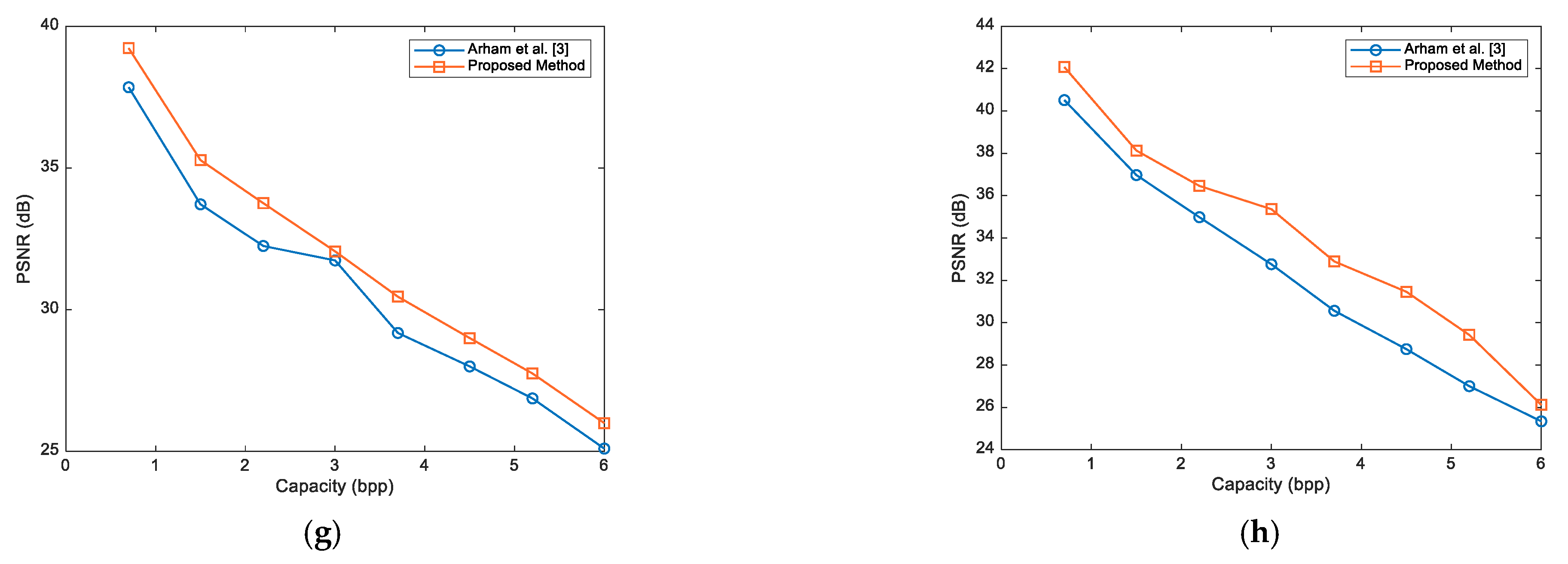Figure 7 shows a comparison diagram of the capacity and PSNR values of the proposed method and the method of Arham et al. [3] for eight insertion layers drawn using the data shown in Table 5.

Table 6. Comparison of the SSIM in common images for different capacities.

	Proposed		Insertion Capacity (bits)			SSIM
Image	T1	T2	[3]	[24]	PM	[3]	[24]	PM
Airplane	111	182	194,250	210,000	215,000	0.9128	0.9131	0.9261
Baboon	78	149	193,314	110,000	195,003	0.9125	0.9155	0.9298
Barbara	55	131	191,466	158,000	192,232	0.9135	0.9146	0.9283
Ship	79	156	194,583	160,000	196,144	0.9134	0.9124	0.9282
Lena	85	152	196,768	200,000	209,000	0.9132	0.9138	0.9272
Lake	76	145	191,854	111,000	193,458	0.9157	0.9115	0.9284
Bridge	84	151	192,472	185,000	196,874	0.9125	0.9114	0.9279
Cameraman	91	174	194,968	159,000	199,762	0.9148	0.9118	0.9256
Peppers	61	136	195,414	178,000	196,985	0.9136	0.9145	0.9274

PM = proposed method.

shows the SSIM values of the proposed method and the methods of Arham et al. [3] and Kumar et al. [16] for maximum embedding capacity (bits). According to Table 6, due to its nature, the proposed method has a higher SSIM than the compared methods, while the capacity of the proposed method is also more than that of the compared methods.

Table 7. A comparison of the SSIM for single-layer embedding.

		SSIM
		0.1 bpp	0.2 bpp	0.3 bpp	0.4 bpp	0.5 bpp	0.6 bpp	0.7 bpp
Airplane	[3]	0.9736	0.9658	0.9531	0.9462	0.9312	0.9243	0.9134
	Proposed	0.9865	0.9736	0.9638	0.9582	0.9462	0.9365	0.9245
Baboon	[3]	0.9735	0.9685	0.9538	0.9425	0.9365	0.9235	0.9141
	Proposed	0.9846	0.9734	0.9648	0.9536	0.9468	0.9328	0.9267
Barbara	[3]	0.9762	0.9694	0.9539	0.9462	0.9361	0.9217	0.9119
	Proposed	0.9873	0.9725	0.9647	0.9543	0.9486	0.9369	0.9278
Ship	[3]	0.9748	0.9657	0.9567	0.9474	0.9313	0.9236	0.9167
	Proposed	0.9839	0.9746	0.9625	0.9512	0.9452	0.9385	0.9286
Lena	[3]	0.9743	0.9651	0.9512	0.9436	0.9321	0.9238	0.9118
	Proposed	0.9849	0.9783	0.9674	0.9572	0.9445	0.9368	0.9264
Lake	[3]	0.9739	0.9645	0.9536	0.9412	0.9336	0.9225	0.9136
	Proposed	0.9818	0.9762	0.9652	0.9548	0.9462	0.9368	0.9275
Bridge	[3]	0.9786	0.9638	0.9536	0.9438	0.9356	0.9283	0.9169
	Proposed	0.9863	0.9782	0.9671	0.9582	0.9468	0.9397	0.9247
Cameraman	[3]	0.9768	0.9637	0.9532	0.9413	0.9367	0.9214	0.9179
	Proposed	0.9864	0.9726	0.9682	0.9551	0.9439	0.9369	0.9264
Peppers	[3]	0.9739	0.9632	0.9539	0.9462	0.9363	0.9258	0.9179
	Proposed	0.9827	0.9746	0.9648	0.9583	0.9486	0.9378	0.9248

PM = proposed method.

shows the method proposed by Arham et al. [3], using the SSIM evaluation metric, which compares one embedding layer and several embedding layers. As can be seen in Table 7, the proposed method has superior performance for different capacities (bpp) compared to the method of Arham et al. [3], with a higher SSIM value. As the capacity value increases in bpp, the SSIM value for the proposed method and the method of Arham et al. [3] decreases. Still, in any case, the proposed method compared is superior to the method of Arham et al. [3] in terms of SSIM value.

Table 8. Compares the PSNR value for the PM and yao et al. [22] method.

	30,000 (bits)				50,000 (bits)
	psnr		ssim		psnr		ssim
Image	Yao et al. [30]		PM		Yao et al. [30]		PM
Airplane	65.56	0.9736	66.12	0.9846	64.34	0.9616	65.22	0.9765
Baboon	65.56	0.9747	66.68	0.9874	64.34	0.9623	65.44	0.9716
Barbara	65.56	0.9732	66.23	0.9834	64.34	0.9675	65.65	0.9736
Ship	65.56	0.9747	66.42	0.9845	64.34	0.9646	65.61	0.9765
Lena	65.56	0.9761	66.29	0.9856	64.34	0.9654	65.12	0.9748
Lake	65.42	0.9719	66.18	0.9885	64.12	0.9638	65.83	0.9716
Bridge	65.56	0.9764	66.47	0.9849	64.34	0.9676	65.79	0.9734
Cameraman	65.55	0.9773	66.42	0.9859	64.34	0.9649	65.68	0.9756
Peppers	65.56	0.9772	66.82	0.9817	64.34	0.9647	65.36	0.9748

PM = proposed method.

shows the PSNR and SSIM values for the proposed method and the method of Yao et al. [30] for capacities of 30,000 and 50,000 bits. As can be seen from Table 8, the proposed method has higher SSIM and PSNR values compared to the method of Yao et al. [30].

In this paper, a multilayer RDH method based on the multilevel thresholding technique is proposed, aiming to increase the insertion capacity and reduce the distortion after data embedding by improving the correlation between consecutive pixels of the image. Firstly, the SMA is applied to find the optimal thresholds of host image segmentation. Next, according to the specified threshold, image pixels located in different image areas are classified into different categories. Finally, the difference between two consecutive pixels is reduced in each class, and then the data are embedded via DE.

4. Conclusions

In this paper, a new multilayer RDH technique was proposed using multilevel thresholding where, first, the SMA was used to determine the optimal thresholds on the host image. By using the SMA, two optimal threshold values were determined. Image pixels were then located in their specific classes based on those thresholds. The similar and more correlated pixels within a group were classified. Therefore, the difference between pixels related to each class decreased. It was proven that insertion and distortion in the marked image decreased after inserting the data by reducing the differences between each class’ pixels. The proposed method has a simple implementation. The results showed that the proposed method, in comparison with the methods of Arham et al. [3] and Kumar et al. [24], has more capacity and more PSNR, but is slightly slower in comparison with the methods of Arham et al. [3] and Kumar et al. [24]. In our subsequent work, we intend to use deep learning methods to extract features and image thresholds in order to classify image features and maximize the capacity and quality of the marked image. Therefore, using the multilevel thresholding technique in the proposed method improved the multilayer RDH method compared to the other methods. This technique reduced the difference between the pixels, and the pixels in the same class were very similar to one another.

References

1. Abdullah, S.M.; Manaf, A.A. Multiple Layer Reversible Images Watermarking Using Enhancement of Difference Expansion Techniques; Springer: Berlin/Heidelberg, Germany, 2010; Volume 87, pp. 333–342. [Google Scholar]
2. Zeng, X.; Li, Z.; Ping, L. Reversible data hiding scheme using reference pixel and multi-layer embedding. Int. J. Electron. Commun. (AEÜ) 2012, 66, 532–539. [Google Scholar] [CrossRef]
3. Arham, A.; Nugroho, H.A.; Adji, T.B. Multiple Layer Data Hiding Scheme Based on Difference Expansion of Quad. Signal Process. 2017, 137, 52–62. [Google Scholar] [CrossRef]
4. Maniriho, P.; Ahmad, T. Information Hiding Scheme for Digital Images Using Difference Expansion and Modulus Function. J. King Saud Univ. Comput. Inf. Sci. 2018, 31, 335–347. [Google Scholar] [CrossRef]
5. Yao, H.; Qin, C.; Tang, Z.; Tian, Y. Guided filtering based color image reversible data hiding. J. Vis. Commun. Image R 2013, 43, 152–163. [Google Scholar] [CrossRef]
6. Ou, B.; Li, X.; Zhao, Y. Pairwise Prediction-Error Expansion for Efficient Reversible Data Hiding. IEEE Trans. Image Process. 2013, 22, 5010–5021. [Google Scholar] [CrossRef] [PubMed]
7. Li, X.; Zhang, W.; Gui, X.; Yang, B. Efficient Reversible Data Hiding Based on Multiple Histograms Modification. IEEE Trans. Inf. Forensics Secur. 2015, 10, 2016–2027. [Google Scholar]
8. Fu, D.; Jing, Z.J.; Zhao, S.G.; Fan, J. Reversible data hiding based on prediction-error histogram shifting and EMD mechanis. Int. J. Electron. Commun. 2014, 68, 933–943. [Google Scholar] [CrossRef]
9. Ou, B.; Li, X.; Wang, J.; Peng, F. High-fidelity reversible data hiding based on geodesic path and pairwise prediction-error expansion. Neurocomputing 2016, 68, 933–943. [Google Scholar] [CrossRef] [Green Version]
10. Wang, J.; Ni, J.; Zhang, X.; Shi, Y.Q. Rate and Distortion Optimization for Reversible Data Hiding Using Multiple Histogram Shifting. IEEE Trans. Cybern. 2016, 47, 315–326. [Google Scholar] [CrossRef]
11. Xiao, M.; Li, X.; Wang, Y.; Zhao, Y.; Ni, R. Reversible data hiding based on pairwise embedding and optimal expansion path. Signal Process. 2019, 19, 30017–30019. [Google Scholar] [CrossRef]
12. Zhou, H.; Chen, K.; Zhang, W.; Yu, N. Comments on Steganography Using Reversible Texture Synthesis. IEEE Trans. Image Process. 2017, 26, 1623–1625. [Google Scholar] [CrossRef] [PubMed]
13. Shehab, M.; Abualigah, L.; Shambour, Q.; Abu-Hashem, M.A.; Shambour, M.K.Y.; Alsalibi, A.I.; Gandomi, A.H. Machine learning in medical applications: A review of state-of-the-art methods. Comput. Biol. Med. 2022, 145, 105458. [Google Scholar] [CrossRef] [PubMed]
14. Zhu, X.; Zhou, M. Multiobjective Optimized Cloudlet Deployment and Task Offloading for Mobile-Edge Computing. IEEE Internet Things J. 2021, 8, 15582–15595. [Google Scholar] [CrossRef]
15. Zhu, Q.-H.; Tang, H.; Huang, J.-J.; Hou, Y. Task Scheduling for Multi-Cloud Computing Subject to Security and Reliability Constraints. IEEE/CAA J. Autom. Sin. 2021, 8, 848–865. [Google Scholar] [CrossRef]
16. Ezugwu, A.E.; Ikotun, A.M.; Oyelade, O.O.; Abualigah, L.; Agushaka, J.O.; Eke, C.I.; Akinyelu, A.A. A comprehensive survey of clustering algorithms: State-of-the-art machine learning applications, taxonomy, challenges, and future research prospects. Eng. Appl. Artif. Intell. 2022, 110, 104743. [Google Scholar] [CrossRef]
17. Otair, M.; Abualigah, L.; Qawaqzeh, M.K. Improved near-lossless technique using the Huffman coding for enhancing the quality of image compression. Multimed. Tools Appl. 2022, 1–21. [Google Scholar] [CrossRef]
18. Tang, J.; Liu, G.; Pan, Q. A Review on Representative Swarm Intelligence Algorithms for Solving Optimization Problems: Applications and Trends. IEEE/CAA J. Autom. Sin. 2021, 8, 1627–1643. [Google Scholar] [CrossRef]
19. Abualigah, L.; Abd Elaziz, M.; Sumari, P.; Geem, Z.W.; Gandomi, A.H. Reptile Search Algorithm (RSA): A nature-inspired meta-heuristic optimizer. Expert Syst. Appl. 2022, 191, 116158. [Google Scholar] [CrossRef]
20. He, W.; Cai, J.; Xiong, G.; Zhou, K. Improved reversible data hiding using pixel-based pixel value grouping. Optik 2017, 157, 68–78. [Google Scholar] [CrossRef]
21. He, W.; Xiong, G.; Zhou, K.; Cai, J. Reversible data hiding based on multilevel histogram modification and pixel value grouping. J. Vis. Commun. Image Represent. 2016, 40, 459–469. [Google Scholar] [CrossRef]
22. Li, X.; Li, J.; Li, B.; Yang, B. High-fidelity reversible data hiding scheme based on pixel-value-ordering and prediction-error expansion. Signal Process. 2013, 93, 198–205. [Google Scholar] [CrossRef]
23. Kumar, R.; Jung, K.H. Robust reversible data hiding scheme based on two-layer embedding strategy. Inf. Sci. 2020, 512, 96–107. [Google Scholar] [CrossRef]
24. Kumar, R.; Kim, D.S.; Jung, K.H. Enhanced AMBTC based data hiding method using hamming distance and pixel value differencing. J. Inf. Secur. Appl. 2019, 47, 94–103. [Google Scholar] [CrossRef]
25. Kim, P.H.; Ryu, K.W.; Jun, K.H. Reversible data hiding scheme based on pixel-value differencing in dual images. Int. J. Distrib. Sens. Netw. 2020, 16, 1550147720911006. [Google Scholar] [CrossRef]
26. Hussain, M.; Riaz, Q.; Saleem, S.; Ghafoor, A.; Jung, K.H. Enhanced adaptive data hiding method using LSB and pixel value differencing. Multimed. Tools Appl. 2021, 80, 20381–20401. [Google Scholar] [CrossRef]
27. Yu, C.; Zhang, X.; Zhang, X.; Li, G.; Tang, Z. Reversible Data Hiding with Hierarchical Embedding for Encrypted Images. IEEE Trans. Circuits Syst. Video Technol. 2021, 32, 451–466. [Google Scholar] [CrossRef]
28. Tang, Z.; Nie, H.; Pun, C.M.; Yao, H.; Yu, C.; Zhang, X. Color Image Reversible Data Hiding with Double-Layer Embedding. IEEE Access 2020, 8, 6915–6926. [Google Scholar] [CrossRef]
29. Yao, H.; Mao, F.; Tang, Z.; Qin, C. High-fidelity dual-image reversible data hiding via prediction-error shift. Signal Process. 2020, 170, 107447. [Google Scholar] [CrossRef]
30. Salehnia, T.; Izadi, S.; Ahmadi, M. Multilevel image thresholding using GOA, WOA and MFO for image segmentation. In Proceedings of the 8th International Conference on New Strategies in Engineering, Information Science and Technology in the Next Century, Dubai, United Arab Emirates (UAE), 2021; Available online: https://civilica.com/doc/1196572/ (accessed on 16 March 2022).
31. Raziani, S.; Salehnia, T.; Ahmadi, M. Selecting of the best features for the knn classification method by Harris Hawk algorithm. In Proceedings of the 8th International Conference on New Strategies in Engineering, Information Science and Technology in the Next Century, Dubai, United Arab Emirates (UAE), 2021; Available online: https://civilica.com/doc/1196573/ (accessed on 16 March 2022).
32. Salehnia, T.; Fath, A. Fault tolerance in LWT-SVD based image watermarking systems using three module redundancy technique. Expert Syst. Appl. 2021, 179, 115058. [Google Scholar] [CrossRef]
33. El Aziz, M.A.; Ewees, A.A.; Hassanien, A.E. Whale Optimization Algorithm and Moth-Flame Optimization for Multilevel Thresholding Image Segmentation. Expert Syst. Appl. 2017, 83, 242–256. [Google Scholar] [CrossRef]
34. Akay, B. A study on particle swarm optimization and artificial bee colony algorithms for multilevel thresholding. Appl. Soft Comput. 2013, 13, 3066–3091. [Google Scholar] [CrossRef]
35. Li, S.; Chen, H.; Wang, M.; Heidari, A.A.; Mirjalili, S. Slime mould algorithm: A new method for stochastic optimization. Future Gener. Comput. Syst. 2020, 111, 300–323. [Google Scholar] [CrossRef]
36. Liu, H.; Zhou, M.; Guo, X.; Zhang, Z.; Ning, B.; Tang, T. Timetable Optimization for Regenerative Energy Utilization in Subway Systems. IEEE Trans. Intell. Transp. Syst. 2019, 20, 3247–3257. [Google Scholar] [CrossRef]
37. Abualigah, L.; Yousri, D.; Abd Elaziz, M.; Ewees, A.A.; Al-Qaness, M.A.; Gandomi, A.H. Aquila optimizer: A novel meta-heuristic optimization algorithm. Comput. Ind. Eng. 2021, 157, 107250. [Google Scholar] [CrossRef]
38. Agushaka, J.O.; Ezugwu, A.E.; Abualigah, L. Dwarf mongoose optimization algorithm. Comput. Methods Appl. Mech. Eng. 2022, 391, 114570. [Google Scholar] [CrossRef]
Figure 1. Production of vectors for four layers [3]: (a) Layer-1; (b) Layer-2; (c) Layer-3; (d) Layer-4.
Processes 10 00858 g001
Figure 2. Production of the matrices for three classes: (a) Class C 1 ; (b) Class C 2 ; (c) Class C 3 .
Processes 10 00858 g002
Figure 3. Production of the vector P.
Processes 10 00858 g003
Figure 4. An example of quad-pixel reversible data embedding: (a) before embedding; (b) after embedding; (c) after extraction.
Processes 10 00858 g004
Figure 5. Used host images in this paper: (a) Lena; (b) Peppers; (c) Airplane; (d) Baboon; (e) Ship; (f) Barbara; (g) Cameraman; (h) Lake; (i) Bridge.
Processes 10 00858 g005
Figure 6. Comparison of image quality for single-layer capacity: (a) Airplane; (b) Baboon; (c) Barbara; (d) Ship; (e) Lena; (f) Peppers; (g) Lake; (h) Bridge [3].
Processes 10 00858 g006aProcesses 10 00858 g006b
Figure 7. Comparing the quality values for multilayer capacities in different images: (a) Airplane; (b) Baboon; (c) Barbara; (d) Ship; (e) Lena; (f) Peppers; (g) Lake; (h) Bridge [3].
Processes 10 00858 g007aProcesses 10 00858 g007b