
Using a Machine Learning Regression Approach to Predict the Aroma Partitioning in Dairy Matrices †
by
 , , and
Marvin Anker
1 ,
,
Christine Borsum
1,2,
Youfeng Zhang
3,
Yanyan Zhang
3 and
Christian Krupitzer
1,* 1
Department of Food Informatics and Computational Science Hub, University of Hohenheim, 70599 Stuttgart, Germany
2
Department of Process Engineering (Essential Oils, Natural Cosmetics), University of Applied Sciences Kempten, 87435 Kempten, Germany
3
Department of Flavor Chemistry, University of Hohenheim, 70599 Stuttgart, Germany
*
Author to whom correspondence should be addressed.
†
Extended version of a paper “Prediction of Aroma Partitioning Using Machine Learning” presented at the 2nd International Electronic Conference on Processes: Process Engineering—Current State and Future Trends (ECP 2023), 17–31 May 2023; Available online: https://0-www-mdpi-com.brum.beds.ac.uk/2673-4591/37/1/48.
Processes 2024, 12(2), 266; https://0-doi-org.brum.beds.ac.uk/10.3390/pr12020266
Submission received: 18 December 2023
/
Revised: 12 January 2024
/
Accepted: 19 January 2024
/
Published: 26 January 2024
(This article belongs to the Special Issue Selected Papers from the 2nd International Electronic Conference on Processes: Process Engineering—Current State and Future Trends (ECP2023))
Abstract
:Aroma partitioning in food is a challenging area of research due to the contribution of several physical and chemical factors that affect the binding and release of aroma in food matrices. The partition coefficient measured by the value refers to the partition coefficient that describes how aroma compounds distribute themselves between matrices and a gas phase, such as between different components of a food matrix and air. This study introduces a regression approach to predict the value of aroma compounds of a wide range of physicochemical properties in dairy matrices representing products of different compositions and/or processing. The approach consists of data cleaning, grouping based on the temperature of analysis, pre-processing (log transformation and normalization), and, finally, the development and evaluation of prediction models with regression methods. We compared regression analysis with linear regression (LR) to five machine-learning-based regression algorithms: Random Forest Regressor (RFR), Gradient Boosting Regression (GBR), Extreme Gradient Boosting (XGBoost, XGB), Support Vector Regression (SVR), and Artificial Neural Network Regression (NNR). Explainable AI (XAI) was used to calculate feature importance and therefore identify the features that mainly contribute to the prediction. The top three features that were identified are log P, specific gravity, and molecular weight. For the prediction of the in dairy matrices, scores of up to 0.99 were reached. For 37.0 C, which resembles the temperature of the mouth, RFR delivered the best results, and, at lower temperatures of 7.0 C, typical for a household fridge, XGB performed best. The results from the models work as a proof of concept and show the applicability of a data-driven approach with machine learning to predict the value of aroma compounds in different dairy matrices.
1. Introduction
Two significant issues facing contemporary societies are diet-related health conditions and global climate change. These issues are prompting shifts in food composition. First, to mitigate health risks and expenses linked to cardiovascular diseases, obesity, and diabetes, it is necessary to reduce the levels of fat, salt, and sugar in our diets. Second, there is a trend toward replacing animal-based proteins with plant-based proteins due to animal welfare and environmental concerns. However, lasting changes in dietary habits are contingent on alternative products replicating the sensory qualities of their traditional counterparts. Therefore, comprehending how changes in composition affect aroma perception is crucial for addressing today’s global challenges.
Extensive research has been conducted on the topic of aroma release to explain the perception formed in the brain. Aroma perception is a complex phenomenon as it depends on physiological parameters showing large inter-individual differences (e.g., saliva, breathing) [1], and it shows cross-modalities with our other sensory inputs, i.e., texture and taste. However, from the food perspective, the release mainly depends on the interactions between aroma compounds and ingredients of the food (fat, carbohydrates, proteins, etc.) and the food environment (pH, temperature). The strength of these interactions can be quantified by the partition coefficient, defined as the quotient between the aroma concentration in the food and the concentration in the headspace above the food [1]. The value is determined in equilibrium; thus, it describes the thermodynamic end state. However, it also determines the kinetics of aroma release as the release rate is higher for aroma compounds showing weak interactions with the matrix [2].
Altering a food’s composition, such as reducing its fat content, significantly impacts its aroma profile due to the varying interactions each aroma compound has with the fat phase [3]. Understanding the value of these compounds in the altered composition is essential. This knowledge, combined with the concentration of the aroma compound in the food, allows for the estimation of the aroma concentration that may be released during consumption [4]. Predicting how aroma partition changes with composition alterations is key to the acceptance of these reformulated food products [5,6,7,8].
In the realm of food technology, while basic physical principles are often understood, the complexity of food matrices necessitates a largely empirical approach to research [9,10,11,12,13,14]. Machine learning offers a solution to bridge this gap as it can integrate foundational knowledge with extensive empirical datasets to create predictive models. Comprehending these models is vital for applying insights to the development of foods that are both healthy and sustainable. Machine learning has shown a good result in similar applications of food processing [15,16,17]; however, it has not yet been applied in aroma perception.
In our previous publication, we described a concept for aroma prediction using machine learning and explainable artificial intelligence (XAI) [18]. This article provides the first exploratory analysis of this concept. It extends the previous publication by showing how to apply the concept using machine-learning-based regression (This paper integrates parts of the previous publication [18] in Section 2 and Section 3. Section 4, Section 5 and Section 6 contain solely completely new content), if you insist to keep this information, please kindly move this part to Section 1 of this manuscript). Hence, we present an approach for establishing a regression model that uses machine learning to predict the value of aroma compounds in dairy matrices. Additionally, we conduct extensive literature research on the current state of aroma binding modeling. We further utilize explainable artificial intelligence (XAI) to explain the results of the machine learning analysis. The insights from this study will be the basis to further develop a universal aroma interaction prediction model that allows for fast and easy reformulation of food products.
The remainder of this paper is structured as follows. After this introduction, we describe relevant concepts in Section 2: aroma–matrix interaction, prediction of aroma–matrix interactions, and machine learning. We give an overview of the current research in the fields of aroma binding and XAI in Section 3. Then, Section 4 describes the proceedings to create the regression models. Section 5 presents the evaluation of the models and critically analyzes the results, exploring their implications for the broader field. Furthermore, we consider any limitations of the study and suggest avenues for future research. Finally, Section 6 concludes with deriving future work.
2. Background
In this section, we present several important concepts for understanding the remainder of the paper. The topics include overviews on aroma–matrix interaction, approaches to predict the aroma–matrix interaction, and the basics of machine learning.
2.1. Aroma–Matrix Interaction
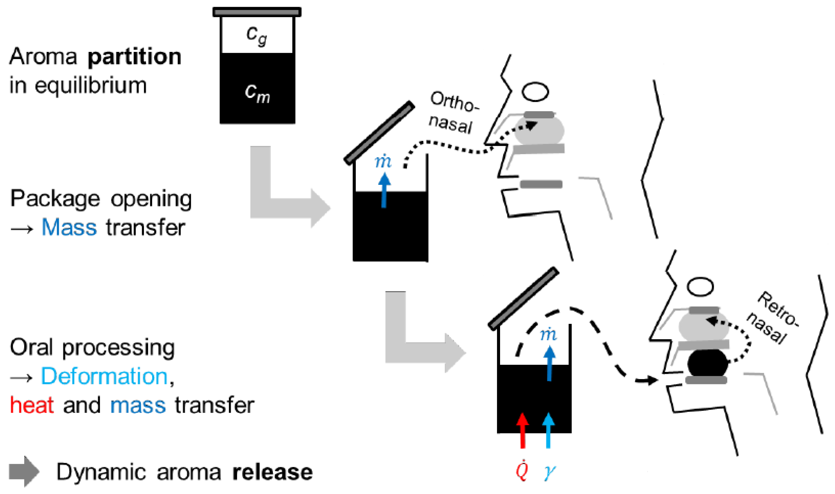
Aroma compounds can interact with food ingredients in different ways; interactions such as hydrogen bonds, electrostatic interactions, van der Waals, or hydrophobic interactions, being the most common ones, will be the focus of this project, as they determine the aroma perception of food [3]. Figure 1 illustrates the following different processes involved during the aroma release from a food:
- Static Aroma Release: The aroma partition coefficient describes the state in closed packaging; therefore, the first orthonasal impression of the food is determined by the aroma concentration in the headspace ;
- Dynamic Aroma Release: During oral processing, the food is cooled down or warmed up to a physiological temperature, mixed with saliva, and mechanically processed [4].
These processes lead to a fast release of the reversibly bound aroma compounds in the food (), leading to retronasal aroma perception. This is why knowing real concentrations in the matrix and headspace, calculated from the value, is the basis for the development of reformulated foods with a similar aroma perception to the original.
2.2. Prediction of Aroma–Matrix Interactions
Aroma–matrix interactions depend on the chemical properties of the aroma compound on the one hand and the composition and processing of the food on the other. In a nutshell, all prediction models are built up similarly. First, the dominating mechanism of interaction with the studied food compound is determined, e.g., hydrogen binding or hydrophobic interactions. Second, a coefficient needs to be found that quantifies the ability of the aroma compound for these interactions. In the case of hydrophobic interactions, this is often the log P value [19], which describes the logarithmic partition ratio between octanol () and water () (see Equation (1)). The log P is a dimensionless measure for the ratio of a compound’s concentrations in two immiscible phases. It is crucial for understanding the lipophilicity of a molecule. The concentration of octanol and water for the relation is measured in mg/kg. Moreover, the carbon chain length of the organic molecules is a relevant parameter for hydrophobicity [10].
Third, the method of partial least square regression (PLSR) is used to find the correlation function to link the coefficients with the correct weights to the output, the value. This method is called the quantitative structure property or activity relationship (QSPR or QSAR) [20,21] as it uses the information of the chemical structure to predict a coefficient of functionality, in this case, the aroma–matrix interaction.
The influence of food ingredients on the value has also been extensively studied [3]; however, most studies were conducted focusing on one ingredient, for example, -lactoglobulin [19,22]. However, this knowledge is only a basis for understanding aroma–matrix interactions of complex food. Reformulating foods needs a model able to describe and compare aroma partition in real foods containing lipids, proteins, carbohydrates, salts, and water. Fat, for example, can bind many more aroma compounds than proteins [23,24]. Additionally, the inclusion of a gas phase also significantly changes aroma binding in foods [2]. This is why the number of parameters influencing aroma–matrix interactions in real foods is larger than that in the simplified models described in the scientific literature.
In addition to the compositional complexity, food processing also influences aroma–matrix interactions. Heating steps influence protein conformation, thus influencing possible binding sites of aroma compounds [5,6]. Microbiological fermentation steps are also relevant as they often decrease the pH value. If electrostatic interactions bind aroma compounds, they will be affected by changes in pH [7]. Additionally, the protein conformation depends on pH if denaturation takes place. This process can also be caused by changes in salt content [8].
2.3. Machine Learning Basics
Machine learning methods are used to find and describe relationships between different attributes in a large dataset to predict, classify, or forecast one or more output parameters. In this paper, we focus on supervised machine learning techniques. Hence, we apply an existing dataset with various variables, called features, and define one dataset as the class. In the case of regression, which is the focus of this work, the class is a numerical value. The machine learning algorithm then follows a specific defined approach to determine patterns between the values of the features and the corresponding value of the class. Using those patterns, the learner defines a machine learning model, which can be later used by feeding in new data and predicting the value for the class. In this paper, the features of the machine learning models are measurements of chemical analyses and compounds. As a class, we set the measured value.
A typical machine learning pipeline includes the following process steps. First, the relevant data must be gathered. Second, the data must be inspected and potentially cleaned, i.e., by handling missing values, removing duplicates, and correcting errors. Further, pre-processing the data, e.g., through normalization or transformation of variables, improves the data quality. Third, feature selection and engineering support the selection of the most relevant features and potentially create new features to improve model performance. Fourth, the data are divided into datasets for training and testing to ensure the model can be evaluated on unseen data. Then, the training of the models starts by choosing appropriate machine learning algorithms and training the models on the training dataset, adjusting parameters as necessary. Finally, the models’ performance is evaluated on the testing set using appropriate metrics (like accuracy, precision, recall, and F1 score for classification problems or Coefficient of Determination (), Mean Absolute Error (MAE), and Root-Mean-Squared Error (RMSE) for regression). We will describe the implementation of these steps for our study in detail in Section 4.
3. Related Work
In the following, we discuss related work. The section is separated into two subsections. First, we explore research in the field of aroma partitioning that is relevant to this study. Second, we discuss machine learning applications for food processing that exhibit an additional value.
3.1. Modeling Aroma Partitioning
First, we introduce studies that show the current research within the intersection of olfactometry and machine learning. Lötsch et al. [25] showed applications of olfactometric data with a set of unsupervised and supervised algorithms for pattern-based odor detection and recognition, odor prediction from physicochemical properties of volatile molecules, and knowledge discovery in publicly available big databases. Two different approaches to predict the structure–odor relationship with machine learning were conducted by Schicker et al. [26]—who developed a classification algorithm that quantitatively assigns structural patterns to odors—and Bo et al. [27], who used deep learning on the structural features for a binary two-class prediction of the odors. It was possible for Lee et al. [28] to generate a principal odor map by constructing a message passing an artificial neural network (NN) to map chemical structures to odor percepts that enable odor quality prediction with human-level odor description performance and outperform chemoinformatic models. The principal odor map represents perceptual hierarchies and distances and can detect previously undetected odorants.
The approach using several machine learning regression methods as powerful tools that can significantly reduce the time and resources needed to simulate complex systems is established in many scientific fields, as shown by Jain et al. [29], who used an array of ML regressors to forecast the performance of microwave absorption. In contrast, the amount of research on aroma partitioning using machine learning regression methods is limited. In the following, we give an overview of the field of matrix–flavor interactions. The hill models [9] are the basis for describing a flavor compound with proteins under equilibrium conditions. These have been advanced by constructing models that use PLSR as a function of the molecular descriptors [10]. Further, a mathematical model for flavor partitioning in protein solutions has been developed and employed for a practical dairy system by Viry et al. [11]. Weterings et al. [12] classified the different behavior of aroma release based on models of interfacial mass transfer. The mechanistic knowledge from mass transfer and aroma release kinetics is used to explain the impact of viscosity on aroma release. Zhang et al. [13] elaborated on the effects of protein properties and environmental conditions on flavor–protein interactions. The binding behavior of flavors to all major food ingredients and their influences on flavor retention, release, and perception were collected by Chen et al. [14]. In terms of improving the quality of food reformulation, they showed practical approaches to manipulating interactions.
Many individual studies have determined the partition coefficient for different combinations of plant proteins and aroma compounds [30,31,32,33]. Although many studies have explored these interactions, modeling the aroma partitioning of plant-based proteins has only recently been attempted [34,35]. The aroma partitioning models were based on mathematical models contained in [13] and were fitted to experimental data for four plant proteins with a variety of esters, ketones, and aldehydes.
This emphasizes that current research focuses on the exploration of aroma–protein interaction mechanisms but not on the use of underlying data to predict these interactions. To define our research in contrast to that of others, we take one of the few examples that used machine learning to develop aroma prediction models. Wang et al. [36] developed models that can predict the flavor of a specific compound in beer and its retention index value, which is used in gas chromatography to compare and identify compounds. They aimed to determine the relationship between beer flavor and molecular structure with a classification algorithm and use regression models on the relative measure of the retention index for the identification of volatile compounds. Our approach uses a database with physicochemical properties and experimental parameters to predict matrix–aroma interactions on the absolute measure of the to provide insight into the retention mechanism and to achieve an efficient and robust reformulation prediction model. The main difference is that Wang et al. [36] created prediction models to describe and categorize flavors to build a database. In contrast to this, we aim to extract and transfer knowledge from a database to be able to dynamically describe the physicochemical relationships between food matrices and aroma compounds.
3.2. Machine Learning for Food Processing
In the food domain, big data methods are already being applied in several fields, such as agricultural production, product innovation, food quality, and food safety [37]. For example, Internet of Things (IoT) and big data analysis in agriculture can decrease the usage of herbicides by crop and weed imaging [38]. Food safety can be increased by traceability through blockchain technology, which modernizes the supply chain [39], and food waste can be reduced by using intelligent packaging indicating the degree of freshness [40]. Often, these techniques integrate machine learning techniques for data analysis.
Machine learning can hold the key to determining the most influential factors and their dependencies for a complex process such as aroma release, which is influenced by various parameters from the aroma and food side. The physical models predicting aroma release presented so far focus on specific protein–aroma interactions, but real food systems are far more complex. Predictions using more parameters were tried with multiple linear modeling [41]. However, not all aroma compounds could be described successfully due to their non-linear behavior. It was demonstrated that combining PLS and NNs improved the prediction accuracy when predicting whether the consumer would like green tea beverages [42].
To gain insights into the physicochemical relationships that govern aroma release, XAI can be a valuable tool if it is evaluated correctly [43]. In [18], we describe such a concept, integrating XAI for predicting flavor compounds. Until now, XAI has not been implemented to explain models that predict aroma compounds and their interactions, but it has been successfully integrated for approaches in the food sector, such as the detection of food fraud [15] or the quality assessment of coffee beans [16]. In terms of possibilities to predict the aroma release during chewing, a machine learning methodology to anticipate the food structure with classification models was introduced [17]. With this paper, we not only present a machine-learning-based regression analysis of the value, but also discuss the feature importance as a first step towards an XAI approach. This has not been attempted for aroma partitioning. While other studies use modeling to investigate flavor–protein interactions or classify flavor compounds with an ML approach, we use a data-driven approach that aims to explain physicochemical relationships in aroma partitioning. In the following, we describe our approach.
4. Materials and Method
In this section, we describe our approach to aroma prediction based on Food Informatics [44] using artificial intelligence. First, we describe the whole procedure embedded in an approach for food reformulation, as presented in [18]. This approach relies on the prediction of the value as the relevant variable to describe the aroma. Second, we describe the regression approach for determining the value using machine learning as the key contribution of this paper. In Section 5, we present the result of evaluating different regression algorithms.
4.1. Prediction of Aroma Partitioning Using Machine Learning
The approach begins with selecting input parameters based on the physical laws of aroma release, emphasizing the importance of data quality. The accuracy of machine learning models depends heavily on the quality of raw data; therefore, datasets need to be verified by reproducing selected experiments. For instance, variations in results for the value, determined using the phase ratio variation (PRV) method, are expected due to differences in analytical settings like detector sensitivity or sampling method. Since is calculated from the slope of a linear fit and is prone to deviations, this step is crucial.
The next phase involves selecting and optimizing a suitable machine learning algorithm to predict values for various aroma compounds. Given the “No Free Lunch Theorem”, which states that no single machine learning method is universally superior, various algorithms should be compared. The first exploratory analysis of such algorithms for the prediction of the value is the center of this paper, and we will present the implementation detail in the following subsection.
Key goals of the model are not just accurate prediction of values, but also transparency and understanding of the model’s predictions. This is particularly challenging with “black box” models like deep learning algorithms. However, the use of explainable artificial intelligence (XAI) can help infer physicochemical relationships from data-driven models and increase understanding of the model’s results. In this paper, we analyze the interpretability of the results by an analysis of the feature importance of the best-performing machine learning algorithms.
Finally, computational time is a significant consideration in the machine learning process, with continuous validation of the method as it is selected, optimized, and applied. The focus is on learning a generalizable model applicable to various products, provided relevant values and recipes are available, enhancing the model’s utility across different food products.
4.2. Regression Approach
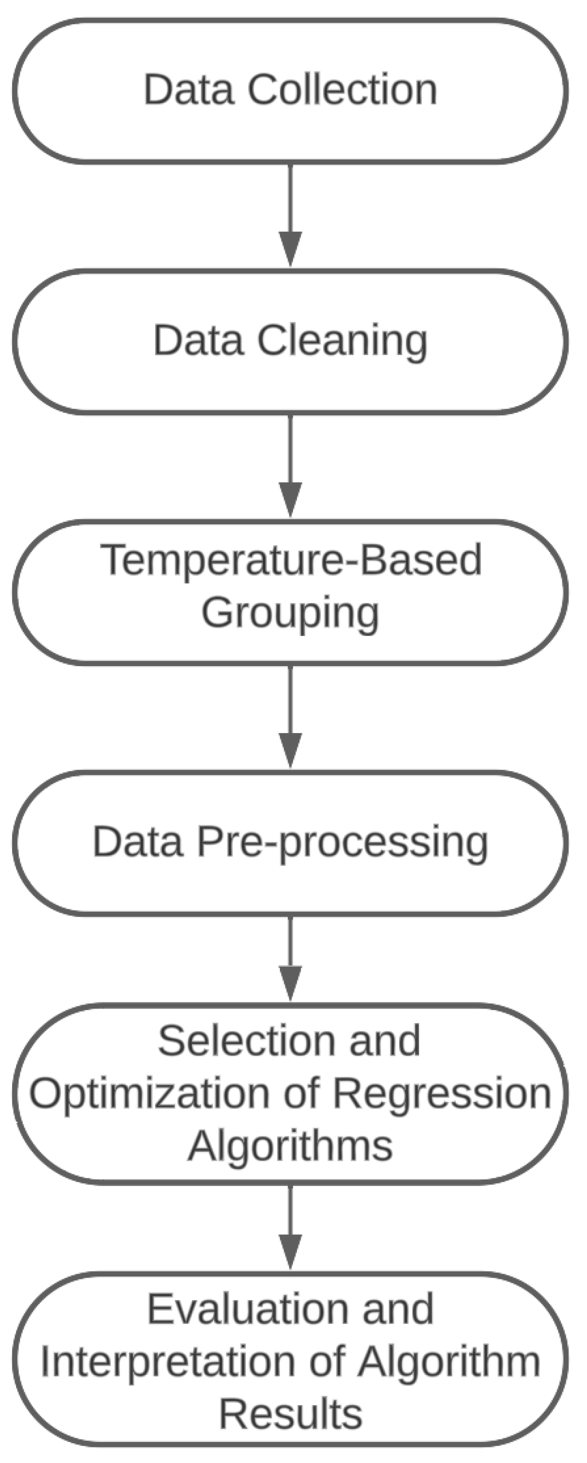
As the value provides an impression of the sensory profile with a single value, we are interested in the composition of the value in dairy matrices for food reformulation. Hence, we followed a machine-learning-based approach for regression of different measurement values to the value. Therefore, we applied a standardized pipeline for the analysis which was composed of the following steps: (i) data collection, (ii) data cleaning, (iii) temperature-based grouping, (iv) pre-processing, and (v) evaluation of regression algorithms. Figure 2 visualizes the workflow of the approach.
In the following, we describe the details of the steps of the pipeline. This includes the data collection (see Section 4.2.1) and data cleaning (see Section 4.2.2), the grouping of data into different clusters according to the temperature (see Section 4.2.3), the pre-processing in the form of log-based data transformation and normalization (see Section 4.2.4), and the applied and evaluated regression algorithms (see Section 4.2.5), as well as details for the implementation of the pipeline using the Python programming language (see Section 4.2.6).
4.2.1. Data Collection
The pipeline begins with acquiring data. We used the data from the publication of Heilig et al. [41]. This dataset focuses on dairy matrices and contains various features, i.e., variables that have been measured in specific studies or experiments as well as the corresponding value for the target variable that we were trying to predict. The dataset provided 22 variables which we integrate as features. In the following, we describe these features and clarify their role in flavor partitioning.
The log P is the logarithm of the partition coefficient, representing the ratio of a compound’s concentrations in two immiscible phases. It is crucial for understanding the lipophilicity of a molecule, which can influence its distribution between hydrophobic and hydrophilic environments. The specific gravity of the aroma compound is the ratio of the density of the substance to the density of a reference substance and provides information about the relative density of a substance, which is relevant to its behavior in different environments. The molecular weight can influence the aroma compound’s physical and chemical properties, including its partitioning behavior and interaction with other substances. Water solubility is the ability of the aroma compound to dissolve in water, impacting its distribution in aqueous solutions. The boiling point can affect the volatility of a substance, which is relevant as it influences how easily an aroma compound may be released. The concentration of an aroma compound is a fundamental factor in flavor perception, and it can influence its partitioning behavior. Water content can affect the solubility and partitioning of flavor compounds. The general protein content can influence the aroma release by exhibiting a binding capacity for aroma compounds, especially whey protein as the fraction of dairy proteins that are not coagulating after rennet addition during cheese production. Whey proteins are water soluble in their native state but sensitive to heat denaturation. This behavior influences their ability to interact with aroma compounds as the conformation change exposes different functional groups of the molecule. Caseins make up the major protein fraction in milk and give all cheese products their texture as their coagulation forms the gel which is transformed into cheese in the further process. Depending on the dairy matrix that is measured, the pH can vary and influence the aroma release depending on how the aroma compounds react to acidic environments. A whole group of features can be summarized as thickening agents; these are agar, carrageen, starch, pectin, and the sum of hydrocolloids. Thickening agents increase the viscosity, which leads to greater retention of volatile compounds within the food matrix. Two additional features are the sugars lactose and sucrose, which influence the solubility and stability of aroma compounds in the food matrix. Mineral interactions with aroma compounds can emerge from the ash content. The effect of the fat content can vary depending on the solubility of the aroma compounds in a fat phase. Similarly, the skim milk and whole milk amounts influence the aroma release depending on their fat contents.
Additionally, the dataset contained the two variables temperature—which we used to separate the dataset into different groups with homogenous temperature—and value, which represents the target variable for the regression.
4.2.2. Data Cleaning
The next step involved cleaning the data, especially removing items with missing data. In the context of machine learning, a “data item” typically refers to a single unit of data that is used as input for machine learning algorithms. In line with many machine learning applications, especially those dealing with structured data (like data in tables or databases), an individual record, i.e., a row in the dataset, is seen as a “data item” in this paper. Hence, we removed rows with missing data. This step is crucial as missing data can lead to inaccurate models and skewed analysis. However, it is important to consider the impact of this removal; if too many data are missing, or if the missing data are not random, this step could introduce bias. We removed only a small fraction of the data and reduced the size of the dataset from 499 to 474 items.
4.2.3. Temperature-Based Grouping
In the publication of Heilig et al. [41], from which we used the dataset, the authors applied a multiple linear regression. However, the performance was not that good. As temperature influences aroma release by affecting the volatility of aroma compounds, increasing their kinetic energy, promoting diffusion, and facilitating the release of compounds from the food matrix, we assumed that temperature is a key variable in the analysis and that its effects were best studied separately. Hence, we decided to divide the dataset into five separate datasets based on temperature values: 4.0 C, 7.0 C, 30.0 C, 37.0 C, and 40.0 C. This kind of stratification can help in understanding how different temperature conditions affect the outcomes or the target variable. We decided to focus on the temperatures 4.0 C, 7.0 C, 30.0 C, 37.0 C, and 40.0 C as (i) for these values, we had the highest number of data, and (ii) these are common temperatures for food cooled in the fridge or consumed by humans (close to the human temperature). Table 1 shows the number of data for each temperature.
4.2.4. Data Pre-Processing
To improve the results of the regression, we applied two pre-processing techniques to the data: logarithmical transformation and normalization. We applied both techniques to the data for all regression algorithms.
Log transformation is a powerful method of transforming highly skewed data into a more normalized dataset. Applying the natural logarithm or any logarithmic base to each data point can stabilize the variance, making the data more suitable for analysis and for various statistical and machine learning models. This transformation is particularly useful when dealing with data that span several orders of magnitude and can help in reducing the effect of outliers. As the value and some other variables follow a log-based scale, we decided to apply the log transformation to it.
Normalization is a scaling technique in which values are shifted and re-scaled so that they end up ranging between 0 and 1. It is also known as Min–Max scaling. Here, the minimum value of a feature becomes 0, the maximum value becomes 1, and all other values are transformed to fall within this range. This technique is useful when the data have varying scales and the algorithm you are using does not make assumptions about the distribution of your data, such as k-nearest neighbors and NNs.
4.2.5. Evaluation of Different Regression Algorithms
Finally, the pipeline involved evaluating the six different regression algorithms on the pre-processed data. For the regression analysis, we applied “traditional” linear regression (LR) and compared it against five machine-learning-based regression algorithms: Random Forest Regressor (RFR), Gradient Boosting Regression (GBR), Extreme Gradient Boosting (XGBoost, XGB), Support Vector Regression (SVR), and Artificial Neural Network Regression (NNR). These different machine learning algorithms are a set of typical algorithms for machine-learning-based regression analysis and reflect different approaches. The algorithms for LR [45], RFR [46], and GBR [47] were implemented using the machine learning library scikit-learn with default hyperparameters. The hyperparameter settings for the XGB, SVR, and NNR are reported in Appendix A (see Table A1). Each algorithm was trained on the datasets, and their performance was evaluated using the appropriate metrics: RMSE, MAE, and score. This comparative analysis helped in identifying the most suitable model(s) for the given data and problem context. In the following, we describe these six algorithms.
Linear regression (LR): In the publication of Heilig et al. [41], from which we used the dataset, the authors applied a linear regression with multiple factors. Linear regression is a statistical method used for predictive analysis. It models the relationship between a dependent variable and one or more independent variables by fitting a linear equation to observed data. The key goal is to find the linear relationship or trend between the variables. For the sake of comparison with Heilig et al. [41], we also applied linear regression as one algorithm. However, the results were not directly comparable as we applied pre-processing to the features and used a temperature-related approach to model each temperature separately.
Random Forest Regressor (RFR): RFR is an ensemble learning method that operates by constructing multiple decision trees during training and outputting the mean prediction of the individual trees. It is effective for regression tasks and is known for its robustness and ability to handle large datasets with higher dimensionality.
Gradient Boosting Regression (GBR): GBR is a machine learning technique for regression problems which builds a model in a stage-wise fashion like other boosting methods but generalizes them by allowing optimization of an arbitrary differentiable loss function. It sequentially builds the model, correcting the errors made by previous models, and is often more powerful than Random Forest.
Extreme Gradient Boosting (XGBoost, XGB): XGBoost is an efficient and scalable implementation of the gradient-boosting framework. It has gained popularity due to its speed and performance. XGBoost provides parallel tree boosting that solves many data science problems in a fast and accurate way.
Support Vector Regression (SVR): SVR applies the principles of Support Vector Machines (SVM) for regression problems. It involves finding the hyperplane in a multidimensional space that best fits the data points. SVR is known for its effectiveness in high-dimensional spaces and its ability to model complex non-linear relationships.
Artificial Neural Network Regression (NNR): NNR is based on NNs, which are inspired by the structure and functions of the human brain. NNR can model complex non-linear relationships between inputs and outputs and is particularly useful in scenarios where the relationship between variables is difficult to model with traditional statistical methods. It is highly flexible and can be adapted to a wide range of regression tasks. The used version of NNR represents a deep learning approach. Such deep learning approaches are very powerful; however, they have limitations regarding their interpretability. Usually, these approaches require a large number of data—still, we wanted to add such an algorithm for comparison due to its computational power.
4.2.6. Implementation
We used the Python programming language for the implementation of the described pipeline, including the pre-processing steps and the algorithms. Ref. [48] provides all scripts.
The dataset originally included 499 data items. After removing the items with missing data, the dataset was reduced to 474 items. We decided to group the data according to their temperature for two reasons. First, the is highly dependent on the temperature. Second, this was confirmed by the first tests on the whole dataset. Accordingly, the datasets were split into various datasets for the different temperatures during the measurements of the value. We chose to concentrate on the temperatures of 4.0 C, 7.0 C, 30.0 C, 37.0 C, and 40.0 C because these temperatures not only had the most data available but also are typical for foods that are refrigerated or consumed by humans, aligning closely with human body temperature. Data filtering and grouping were performed with the relevant functions provided by the Pandas library.
For log transformation, we used the log1p function provided by the NumPy library. Normalization was performed using the MinMaxScaler from scikit-learn.
Especially, we relied on the scikit-learn library for most of the algorithms; this includes the following modules: LinearRegression, RandomForestRegressor, SVR, and GradientBoostingRegressor. For XGBoost, we used the implementation provided by the xgboost module. The NNR followed the implementation provided by the keras.Sequential module from the Tensorflow library.
For the evaluation of the algorithms’ performance, we applied the metrics provided by the metrics module of the scikit-learn library. We followed a train–test split-based approach with a test size of 20%, i.e., we used 80% of the data for training the models and 20% for testing, hence, evaluating the model’s performance. For the analysis of the feature importance for RFR, GBR, XGB, and SVR, we applied the corresponding integrated functions for calculating the importance scores as well as the matplotlib and seaborn modules for plotting the results.
5. Results
In this section, we describe the results of evaluating the algorithm’s performance in predicting the value by applying regression. First, we describe the setting of the evaluation and the applied metrics. Second, we present the results of the algorithms for the three metrics RMSE, MAE, and score. Third, we analyze the importance of the different features for the prediction of the value. In the previous section, we explained the results of the regression models for predicting the value that our tested algorithms generated. Last, we describe potential threats to validity.
5.1. Evaluation Setting and Metrics
We analyzed the performance of the six mentioned algorithms (cf. Section 4.2.5) in predicting the value through regression using a regular working laptop—with an Intel(R) Core(TM) i7-12700H CPU at 2300 MHz, 32 GB RAM, and Microsoft Windows 10 Education as the operating system—for both model training (learning) and model testing (evaluation). This showed lightweight implementation and low resource consumption, even for the more sophisticated machine learning algorithms.
As described in the pipeline of analysis steps (cf. Section 4.2), we focused on five different temperature values: 4.0 C, 7.0 C, 30.0 C, 37.0 C, and 40.0 C. For each of these temperatures, we generated a dedicated dataset composed of measurement data for solely the specified temperature. For each temperature, we compared the data in the original form with the data resulting from the pre-processing steps (i.e., log-based transformation and normalization). Additionally, we applied all six algorithms to the combination of temperature and data variants. Consequently, this resulted in 60 different scenarios for the evaluation. We applied three metrics commonly used for regression problems to evaluate the algorithms’ performance: RMSE, MAE, and score.
MSE is a common metric used for measuring the accuracy of a regression model. It calculates the average of the squares of the errors or deviations, i.e., the difference between the estimator and what is estimated. MSE gives a relatively high weight to large errors (since it squares the errors), which means it can be particularly useful in situations where large errors are undesirable. The Root-Mean-Squared Error (RMSE) is the square root of MSE. It converts the metric back to the same scale as the original data. Like MSE, RMSE gives more weight to larger errors, but its scale is the same as the data, making it more interpretable and easier to relate to the magnitude of the errors. RMSE is often preferred when the goal is to understand the error in terms of the original units of measurement. As we had partly log-based data, we applied RMSE instead of MSE as it gives a performance more interpretable in terms of the original units of the data.
A lower MSE or RMSE value indicates a better fit of the model to the data.
As an additional metric, we used the MAE as it does not penalize large errors disproportionately, making it less sensitive to the influence of outliers. Consequently, the MAE is a metric that gives equal weight to all errors, regardless of their direction or magnitude and allows comparison of the RMSE.
The metric, also known as the coefficient of determination, is a statistical measure that represents the proportion of the variance for the dependent variable that is explained by the independent variables in a regression model. It indicates the goodness of fit of a set of predictions to the actual values. An score of 1 indicates that the regression predictions perfectly fit the data. Values of outside the range of 0 to 1 can occur when the model does not follow the trend of the data, leading to negative values or values greater than 1.
5.2. Machine Learning Regression
The following two tables describe the results of the performance measurements for the six algorithms—LR, RFR, GBR, XGB, SVR, and NNR—for the different temperatures, i.e., 4.0 C, 7.0 C, 30.0 C, 37.0 C, and 40.0 C. Further, we compared the performance of the algorithms using two variants of the datasets, the original data and the data that are pre-processed by applying log-based transformation and normalization (indicated by the appendix “_Proc”).
Next, Table 2 presents the measured scores. As can be seen, we have a wide range of scores from negative values to positive ones close to +1. This indicates that sometimes the algorithms provide very low performance, especially those configurations with a negative score. However, over all scenarios and configurations, we can see that all temperature configurations, except 30.0 C, have an score of at least 0.880, achieving up to almost perfect prediction with .
This indicates that our principal approach works for the prediction of the value.
Additionally to the scores, we analyzed the RMSE as a description of the size of the error terms. Table 3 shows the measured RMSE scores. As can be seen, the RMSE scores lie in general between 13 and 2856. However, one can see that the ranges are highly different depending on the temperature. For example, the temperature of 7.0 C has the most extreme range, with RMSE scores between 792 and 2856; especially, the minimum RMSE value of 792 exceeds the maximum RMSE for all other temperatures. Additionally, the differences between the minimum and maximum RMSE scores for the temperatures 30.0 C and 37.0 C are both around 100. However, the numbers completely differ, with ranges of 13–132 (for 37.0 C) and 301–416 (for 30.0 C). The ranges for 4.0 C and 40.0 C integrate both acceptable values with minimum RMSE scores of 22 (for 4.0 C) and 65 (for 40.0 C) but high maximum RMSE scores of 297 (for 4.0 C) and 335 (for 40.0 C).
Additionally, we also report the measured values for the MAE. While MAE measures the average magnitude of errors in a set of predictions without considering their direction, RMSE penalizes larger errors more severely by squaring the residuals before averaging, thus often highlighting larger discrepancies more prominently. As can be seen in Table 4, the results are pretty similar, epsecially when focusing on the best configurations for each temperature. Except for the temperature of 37.0 C, the same configuration is superior for RMSE and MAE. In the case of 37.0 C, for MAE, the RFR algorithm in the processed variant is superior than the RFR in the non-processed variant—this is vice versa for the RMSE score.
RMSE is preferred over MAE in many scenarios because it is more sensitive to large errors, as it squares the errors before averaging, thus giving greater weight to larger discrepancies. Additionally, RMSE aligns well with many machine learning algorithms that minimize quadratic loss functions, making it more compatible with common optimization techniques used in predictive modeling. As it can further be seen that the results are pretty similar for MAE and RMSE, we decide to focus on RMSE in the following. For interpretation of the RMSE, it makes sense to have an understanding of the range of the values for the value as the target variable for the prediction. Accordingly, we report the minimum and maximum values for the for each temperature as well as the standard deviation in Table 5. Especially, we compare the RMSE values with the standard deviation of the analyzed variable as the standard deviation is a measure of the amount of variation or dispersion in a set of values, and a high standard deviation means the values are spread out over a wider range. Comparing the RMSE to the standard deviation can give an idea of how much of the variability in the data can be explained by the model. As can be seen, the standard deviation and the range between the minimal and maximal RMSE scores for a temperature are often pretty close. However, we can see small differences. If the RMSE of the model is significantly lower than the standard deviation of the data, it suggests that the model has good predictive accuracy. This is achieved for the temperatures 37.0 C and 40.0 C; especially for the temperature of 37.0 C, this indicates a very good fit of the model to the data as the standard deviation is low. In contrast, if the RMSE is close to or greater than the standard deviation, it indicates that your model may not be performing well and is not adding much value over a simple mean-based prediction. This is the case for the temperature of 30.0 C, where the standard deviation is smaller than the RMSE. Further, for the temperature of 4.0 C, the standard deviation (284) is smaller than the largest RMSE score (297); however, the range is wide, with values between 22 and 297. For the temperature of 7.0 C, the standard deviation lies in the range for the RMSE.
It is important to note that this comparison, while useful, has limitations. RMSE is influenced by outliers and can be disproportionately large if the prediction errors have a skewed distribution. Still, it is a first indicator that, especially for the temperature of 37 C, the model delivers good predictions of the value.
In the following, we will analyze in detail two scenarios. First, we compare the performance of the algorithms when the food items have the temperature of a common household fridge, i.e., 7.0 C. Second, we detail how the algorithms perform when the food is heated up to the temperature of the human mouth, i.e., 37.0 C. We decided to focus on these scenarios as (i) both are relevant from a practical point of view for food consumption, and (ii) if the quality of the algorithms varies, it allows us to draw interesting insights to further improve the prediction.
5.2.1. Analyzing the Performance for Chilled Food (at 7.0 C)
Figure 3 shows the measured score for the six algorithms given the temperature of 7.0 C. The detailed results show interesting insights, which we elaborate on in the following.
First, the approach with NNs does not work at all, as can be seen by the negative scores, which indicate that the model does not follow the trend of the data. However, it can be observed that the data pre-processing improves the results. Second, the best results are returned for XGBoost (XGB) with and the Support Vector (SVR) algorithm with . Interestingly, the XGB performs very well on the non-processed dataset and worse on the pre-processed one; for the SVR, the situation is reversed. In general, it can be seen that, apart from the NN approach, all approaches perform well with an for at least one of the two tested variants of the data. However, the pre-processing of the data does not improve the results for most of the algorithms. Here, we need to test and identify further techniques which might improve the results. Still, the two best-performing configurations—SVR on the pre-processed data and XGB on the original data—deliver a very good performance based on the scores.
Another perspective provides the RMSE, which is visible in Table 3. RMSE calculates the root of the average of the squares of the errors or deviations. The minimal values are in line with the scores present for the XGB (non-processed data) and the SVR (pre-processed data). As can be seen, these values seem large, with 792 and 853 as the minimum values of all configurations for the XGB on the non-processed data and the SVR on the processed data, respectively. One explanation for those relatively large errors lies in the data. Some of the variables follow a log distribution and scale. Hence, taking this into account, the large measured error is relieved. Still, for a practical application of the prediction, we need to find approaches to reduce this error, e.g., with additional pre-processing techniques.
5.2.2. Analyzing the Performance for Mouth Temperature (at 37.0 C)
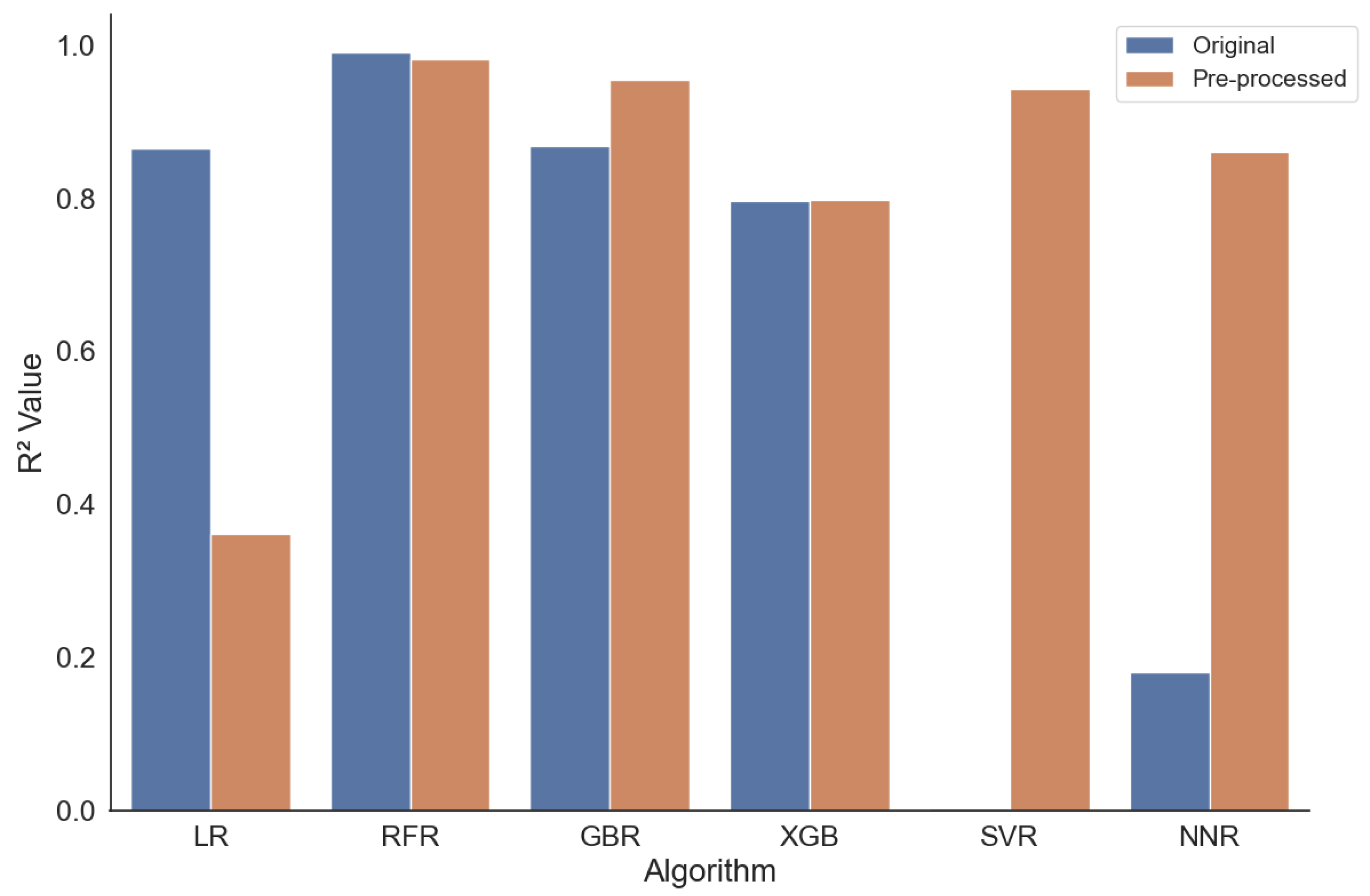
As a second detailed analysis, we focus on the temperature of 37.0 C. Figure 4 compares the measured scores.
As a first observation, it can be stated that all the algorithms work—this time, we have no negative scores. Further, we can observe that, for each algorithm, at least one configuration has a score of . This means that all algorithms are capable of finding a model that explains almost 80% of the variations in the datasets. This is a very impressive result and underlines the fact that the prediction of the value works at a temperature of 37 C, i.e., the temperature of the human mouth, and, hence, predicts the consumers’ impression of the food’s taste.
In detail, we observe very high scores between 0.92 and 0.99 for five configurations. The Random Forest approach performs best with for the non-processed data and for the pre-processed data. Also, the GBR (pre-processed) with , the SVR (pre-processed) with , and the neural network (pre-processed) with deliver a very good performance. The trained/learned models for all of the mentioned configurations explain the variance in the data by at least 92%, especially the performance of the models derived by the RFR algorithms, explaining the variance by 99% and 98%, almost completely.
It is interesting to note that, except for in the case of the RFR, for the mentioned top results, the pre-processed dataset works much better. This is contrary to the observations for the temperature of 7 C, for which the pre-processing mostly does not significantly improve the results. Further, it can be seen that the neural network and SVR approaches benefit from the pre-processing; however, this is not surprising, as neural networks require normalization to work well, and, also, for the SVR, it is known that normalization improves the calculation procedures.
The RMSE for the temperature of 37 C is, in general, relatively low, with values between 13 and 132. Specifically, the error values for the mentioned top-performing algorithms—RFR and RFR (pre-processed), GBR (pre-processed), SVR (pre-processed), and the neural networks (pre-processed)—are very low, with RMSE values of 13, 18, 28, 31, and 37, respectively, which are very good results and support the observation of high prediction quality, which is already indicated by the corresponding scores of these algorithms.
5.2.3. Performance Analysis of the Machine Learning Regression
The described machine learning pipeline (cf. Section 4) represents a comprehensive approach to handling and analyzing data with a focus on addressing specific characteristics of the dataset (like missing values and temperature variations) and evaluating multiple models to find the best fit for the data. The use of pre-processing techniques like log transformation and normalization is particularly important for ensuring that the data are well suited for the modeling process.
We analyze the applied algorithms from different perspectives, resulting in different metrics (cf. Section 5.1). Each of these applied metrics offers a different perspective on the performance of a regression model, and the choice of which to use can depend on the specific context and objectives of the modeling effort. For instance, if large errors are particularly undesirable in a given application, MSE or RMSE might be the preferred metric. If the goal is to simply measure the average error magnitude, MAE might be more appropriate. is useful for understanding the proportion of variance explained by the model in the context of the data. Hence, it is important to understand the use case for the regression and, depending on that, to choose the fitting algorithm and corresponding model. This corresponds to the idea of adaptive software systems, which can integrate adaptive and learning behavior in software to adjust to dynamics [49].
The results (cf. Section 5.2) indicate three important insights. First, the results perform with scores of up to 0.99, which means an explanation of the variance in the data of up to 99%. This is an outstanding result and definitely proves the applicability of our approach for predicting the value.
Second, no algorithm performs best for all settings (e.g., temperatures). This is in line with the “No Free Lunch Theorem” [50], which states that no single algorithm performs best for all problems. For this application domain, this means that the best algorithm/model depends on the temperature of the food. In practice, this insight might be a real challenge, as the food temperature changes, e.g., chilled food will be warmed up in the mouth or, vice versa, hot food will be cooled in the mouth. Hence, food designers who want to use our approach have to take those possible changes into account and need to define the temperature range of interest to identify the fitting regression algorithm. Potentially, a digital food twin might take those changes into account [51]. However, in a current analysis of the digital food twin research, we can see that there are still many research challenges for achieving this [52]. Additionally, the range of tested temperature covers the most important ones—human/mouth temperature and cooling temperature—however, this is limited due to data sparsity. This must be improved for future work.
Third, we applied variants for each algorithm, without optimization and with optimization of the data in the form of pre-processing. However, we have seen that, depending on the configuration and temperature, the pre-processing does not improve the results. For example, for 7.0 C, the best variant is the XGB with the non-processed data. However, there are other settings in which both dataset configurations perform equally well (e.g., temperatures of 37.0 C and 40.0 C) or the pre-processed ones are superior. Especially for the neural network, the pre-processing improves the performance significantly. In contrast, for example, the RFR does not improve much. Consequently, we need further experiments to identify working pre-processing techniques that find the data but also the algorithm’s characteristics.
5.3. Explainable Artificial Intelligence
The objective of the analysis for the value is not only the identification of a prediction of this value, but also the understanding of the influence of the measured factors for describing the value. This understanding is necessary as the results of the prediction will help to reformulate food recipes. Hence, we describe in the following the application of an analysis of the importance of the different factors. We focused in this analysis on the following algorithms: RF, GBR, XGB, and SVR. We excluded the linear regression as those models do not perform best in any of the settings. Further, we excluded the neural networks because they are more difficult to analyze concerning the importance of the variables. We excluded the scenario with a temperature of 30.0 C, as none of the algorithms returns satisfying results.
The method of calculating feature importance can vary. Some common methods include (i) impurity-based feature importance—which measures the decrease in node impurity when a feature is used for splitting—or (ii) permutation feature importance, which involves randomly shuffling each feature and measuring the change in the model’s performance. For the RFR and GBR algorithms, we applied the functions integrated in scikit-learn, which implement an impurity-based feature importance. For XGB, we applied the get_score() method with the parameter gain for the setting importance_type to obtain feature importance scores from an XGBoost model. This method calculates the feature importance scores based on the gain metric. Gain refers to the average improvement in accuracy brought by a feature to the branches it is on. This metric considers both the number of times a feature is used and how much it contributes to making more accurate predictions when it is used. For the SVR algorithm, we applied a weight-based scoring approach. Hence, we manually extracted the scores for each feature from the corresponding model and sorted them from large (more important) to small (less important) values.
Using the described integrated functions for calculating the feature importance of the four mentioned algorithms, we analyzed the ten most important features. First, we present the appearance of specific features in all 16 settings. Hence, Table 6 presents the frequency of the different features appearing in all analyzed settings. The analyzed settings include the four different temperatures of 4.0 C, 7.0 C, 37.0 C, and 40.0 C (excluding 30.0 C). For each temperature, we looked at the applied four algorithms—as mentioned, we excluded the linear regression and the neural network approaches in this analysis. For the temperatures of 4.0 C, 37.0 C, and 40.0 C, we looked at the algorithms using the pre-processed data; for the temperature of 7.0 C, we analyzed the data without pre-processing as, at this temperature, the scores of the data without pre-processing are superior. Consequently, a feature might be named 16 times at maximum in the feature frequency table.
It can be seen that the features log P (100%), specific gravity (93.75%), molecular weight (93.75%), water solubility (87.50%), boiling point (75%), concentration (68.75%), water (68.75%), whey protein (50%), and casein (50%) are the most common features. Their share is determined by how often they are counted as one of the top ten features for the different algorithm and temperature settings. Each feature identified for at least 50% of the setting is marked as being one of the top 10 features for the total 22 analyzed features.
Please note that the frequency shown in Table 6 does not necessarily relate to the features’ importance as it might be possible that features are often named but have low importance. Hence, in the following, we perform a detailed analysis of the importance of the specific features of the algorithms that performed best for each temperature based on the score. We use the seaborn library to plot the results. Feature importance plots are a valuable tool in machine learning for understanding the contribution of each feature (input variable) to the predictive power of a model. These plots help in interpreting the model by quantifying the extent to which each feature contributes to the model’s predictions. The most important features are those that have the greatest impact on the model’s predictions. Please note that, for the different algorithms, the feature importance values are in different scales. Hence, it is not possible to directly compare the absolute values across algorithms.
5.3.1. Explainability in the Best Configurations
First, we analyze the best-performing configurations (according to their score). These are the RFR algorithms with and without pre-processing for the temperature of 37 C. As can be seen from the plots in Figure 5, the most important feature is the specific gravity for both configurations. Interestingly, the feature achieves a score of 0.72 for the setting with the original data, i.e., it contributes 72% to the prediction of the value; all others contribute less than 5% each. For the pre-processed data, the importance of the specific gravity is reduced to 0.53; however, the importance of the feature concentration is 0.27. For both settings, all ten features are identical; however, the importance scores slightly differ.
Other interesting insights are made for the GBR algorithm. For the temperatures of 37.0 C and 40.0 C, the achieved scores are almost the same, both around 0.95; however, different feature sets contribute to the prediction (see Figure 6). In the configuration for the temperature of 37.0 C, the top five most important features are: specific gravity (0.4283), concentration (0.3973), water solubility (0.0550), log P (0.3456), and boiling point (0.0327). In the configuration for the temperature of 40.0 C, the top five most important features are: molecular weight (importance score of 0.3687), log P (0.2461), fat (0.2241), water (0.0502), and specific gravity (0.0320). The top three features are completely different for both settings. Looking at the top five features with the highest importance, both settings share only one common feature; however, the importance of feature log P differs between 0.2461 for the temperature of 40.0 C and 0.3456 for 37.0 C.
For both configurations, we use the pre-processed data; still, there are such differences visible in the feature importance while very good prediction performance is achieved. This underlines the importance of a thorough analysis and interpretation of the models. Further, it indicates the importance of the temperature and the suitability of the temperature-based analysis as we performed it.
5.3.2. Explainability Comparing Pre-Processing Techniques
When focusing on different algorithms for predicting the value for the same temperature, we can see interesting effects. We do not include plots for all of the following settings; however, the results can be found in the online appendix: [48].
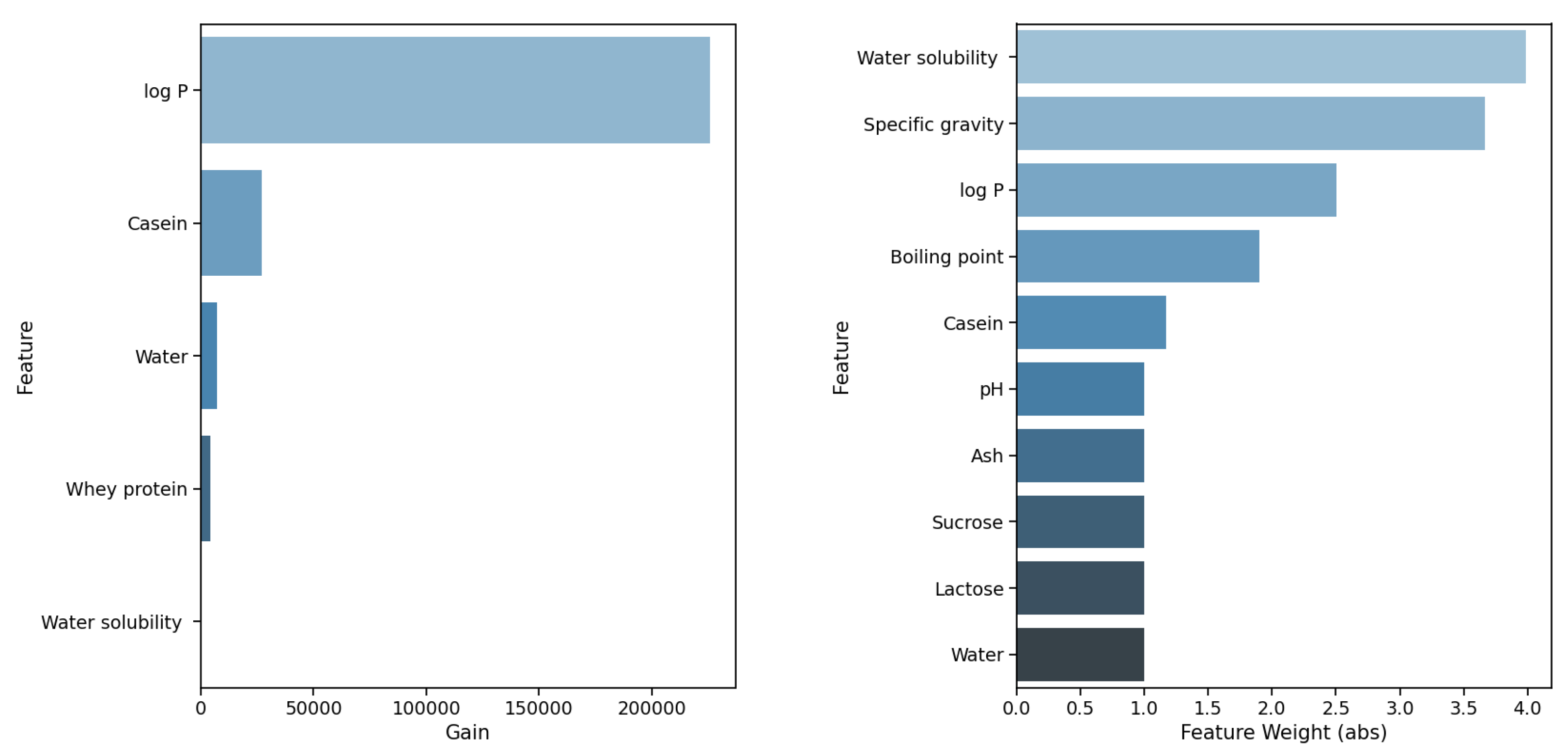
For the temperature of 40.0 C, the algorithms RFR, XGB, and GBR all have the two features fat and log P within the top three features; RFR and GBR even have the same top three features. The same effects can be seen for the temperature of 37.0 C, where SVR, RFR, and GBR all have the same top feature, specific gravity, and all three have concentration as the second or third important feature. GBR and RFR have the same top three features in the same relevance order. In contrast to the more homogenous results for the temperatures of 37.0 C and 40.0 C, the picture changes for the temperature of 7.0 C. Figure 7 shows the result. Please note that, due to the difference in the calculation of the feature importance scores, these scores cannot be compared to the ones in Figure 5 and Figure 6. When focusing on the two best-performing algorithms, XGB and SVR, the first difference that can be observed is the fact that, for XGB, only five features contribute to the result. When comparing both algorithms in detail, it is interesting to note that the most important features completely differ; only the feature log P shows similar importance. Again, this underlines the importance and need for a detailed analysis and interpretation of the models.
5.3.3. Performance Analysis of the Explainable Artificial Intelligence
Explainable artificial intelligence (XAI) refers to methods and techniques in the field of artificial intelligence that make the results and operations of AI systems more understandable to humans. The goal of XAI is to create AI models that are transparent and interpretable, allowing users to comprehend and trust the results and outputs they produce. This is particularly important in this application domain because the main objective is not solely the prediction of the value, but also the understanding of the underlying prediction model so that the model characteristics can help to improve the food reformulation.
In our analysis of the XAI of the tested algorithms (cf. Section 5.3), we had to focus on specific settings for several reasons. First, we omitted the temperature of 30.0 C degrees as the regression results are too low. However, we might still apply XAI to find out why the algorithms do not perform as expected in future work. For this study, this was out of scope as we wanted to learn about the feature that can help to explain the regression of the value. Second, we omitted the linear regression due to its performance. This was also observed by Heilig [41] as they evaluated the model performance for linear regression. Additionally, we plan for the future to transfer the learned model to other food categories in addition to dairy matrices; this does not seem promising with linear regression. Third, artificial neural networks pose significant challenges to XAI due to their inherent complexity and opacity. These challenges primarily stem from the way these neural networks are structured and how they learn to make decisions. Hence, the analysis of the features’ importance is complicated, and, as the NN algorithms also do not outperform the other algorithms, we ignored them for the XAI analysis.
It can be seen that the features log P (100%), specific gravity (93.75%), molecular weight (93.75%), water solubility (87.50%), boiling point (75%), concentration (68.75%), water (68.75%), whey protein (50%), and casein (50%) are the features mostly present, each being identified for at least 50% of the setting as one of the top ten features of the total 22 analyzed features. Further, in the following detailed analysis, we see that the frequently mentioned features often have high feature importance scores; hence, these have relevant effects on the composition of the value.
When comparing the best performers as judged by their scores for the 37 C temperature setting, namely, the RFR both with and without pre-processing, it can be seen that, while the top ten features remain the same in both settings, their respective importance scores vary. This might be an important insight when reformulating food matrices and adjusting recipes.
We can further see that, for the same algorithm, even if the regression performance is very similar in terms of the scores, the temperature plays an important role. The GBR algorithm achieves scores around 0.95 at 37.0 C and 40.0 C yet relies on different feature sets for predictions. While the top three features differ for each temperature, only one feature, log P, is common in the top five, with varying importance between 0.2461 at 40.0 C and 0.3456 at 37.0 C, which confirms our model selection of the important features from the literature. Despite using pre-processed data for both scenarios, the distinct differences in feature importance, coupled with high prediction accuracy, highlight the need for in-depth model analysis and underscore the relevance of temperature in such analyses and also for practical usage.
When analyzing different algorithms for predicting the value at the same temperature, interesting patterns emerge. At 40.0 C, RFR, XGB, and GBR algorithms rank fat and log P among their top three features, with RFR and GBR sharing the same top three. Similar trends are observed at 37.0 C, where SVR, RFR, and GBR all prioritize specific gravity as the top feature and concentration as the second or third. However, at 7.0 C, the results diverge, with XGB and SVR showing distinct differences in feature importance, except for in the case of log P. This emphasizes the need for detailed model analysis and interpretation. Consequently, it is essential to enhance the machine learning process with an XAI component, which can either derive explanations from transparent models or decipher the decision-making process of more complex, opaque models. We describe such an approach in [18]. Its implementation is part of our future work.
Furthermore, the XAI-based analysis shows one obstacle to the data-driven approach. When following a purely data-driven approach, the machine learning algorithm does not take into account specific constraints, for example, from scientific models. In our results, we identify that the feature concentration for the Random Forest with pre-processing at 37 C has a higher importance, as can be explained with scientific knowledge about the chemical interrelationships. Hence, it is important to use the explanations and interpretations from XAI and combine them with domain knowledge for validation. Furthermore, it might be feasible to avoid such wrong conclusions from the machine learning algorithm by integrating the relevant scientific models in advance to set the relevant constraints for the learning process. This could be made possible by integrating surrogate models [53]. Surrogate models are simplified models that are used to approximate more complex and computationally expensive models. They are often employed in various fields such as engineering, simulation, optimization, and machine learning. The primary purpose of a surrogate model is to reduce the computational cost associated with the evaluation of complex models while still providing a reasonably accurate approximation. However, the validation of the XAI or the integration of scientific models into the machine learning process is part of future work.
5.4. Threats to Validity
In evaluating the validity of our scientific study, it is important to acknowledge several limitations and potential threats to the robustness of our findings. We will describe those limitations in the following.
Pre-processing: The use of only basic pre-processing techniques may not adequately address complex data characteristics such as non-linearity, high dimensionality, or hidden patterns, potentially leading to suboptimal model performance and biased results. The inclusion of additional pre-processing techniques is part of our future work. However, the results indicate that the applied techniques work well with the dataset.
Limited number of data: The scarcity of data points, particularly at higher temperature ranges above 40 C, could lead to a lack of representativeness in the dataset, resulting in models that are not well generalized and potentially less accurate in their predictions for these specific conditions. We currently plan further measurements with additional temperature ranges.
Limited set of algorithms: Employing a restricted set of machine learning algorithms may limit the exploration of diverse modeling approaches, potentially overlooking algorithms that could be more effective or suitable for the specific characteristics of the dataset. In this first exploratory study, we focused on only six algorithms. Even though the applied set of algorithms shows good performance, the application of further algorithms is part of future work.
No hyperparameter tuning: The scope of this exploratory study was to identify the applicability of different ML algorithms for prediction of the value using regression; hence, we used the default configurations for these algorithms. Additional hyperparameter tuning can result in models that are better configured for the given data, potentially leading to better performance as compared to models where hyperparameters are not adjusted to enhance their predictive capabilities. It is common practice to rely on the default parameters in a first exploratory study. Further, hyperparameter tuning might also lead to overfitting and reduce the transferability of the machine learning models. However, we plan to integrate hyperparameter tuning in future work for comparison.
6. Conclusions
This study explores the use of machine learning regression to predict the value, a partition coefficient for aroma compounds in dairy matrices, addressing the complex challenge of aroma partitioning in food influenced by various physical and chemical factors. The research aims to demonstrate the feasibility and effectiveness of a data-driven approach in accurately determining the value for aroma compounds using machine-learning-based regression. The results show that, with scores of up to 0.99, the approach is suitable for predicting the value for dairy matrices.
Still, we have open challenges in three facets. First, we were not able to achieve such high results for every single setting. Hence, we might improve the current approach further for better prediction of the value in dairy matrices. This includes more advanced pre-processing techniques, a wider range of machine learning algorithms, implementing feature selection techniques, or hyperparameter tuning. Second, the number of data was limited, especially for larger temperatures. Hence, efforts should be made to collect more data, especially in underrepresented temperature ranges. Additionally, we relied here on a given dataset, for which we were not able to control the creation. Third, we want to transfer the models from dairy products to vegan alternatives based on, e.g., pea, soy, or oak. By establishing the approach, we envision including aroma binding domain knowledge into the models to enable transferability. The idea is that these models will support the development of new products with a fast analysis of an approximation of the sensory profile based on the when adjusting an existing recipe through the substitution of the protein source (milk/animal to plant based). Therefore, we also have to complement the machine learning process with an XAI component, which either extracts explanations directly from transparent models or learns how opaque models arrive at their predictions.
Author Contributions
Conceptualization, C.K., Y.Z. (Yanyan Zhang) and C.B.; methodology, C.K., Y.Z. (Yanyan Zhang) and C.B.; investigation, M.A., C.K., Y.Z. (Yanyan Zhang) and C.B.; resources, M.A.; writing—original draft preparation, M.A. and C.K.; writing—review and editing, M.A., C.K., Y.Z. (Youfeng Zhang), Y.Z. (Yanyan Zhang) and C.B.; visualization, M.A.; supervision, C.K. and C.B. All authors have read and agreed to the published version of the manuscript.
Funding
This research received no external funding.
Data Availability Statement
Conflicts of Interest
The authors declare no conflict of interest.
Abbreviations
The following abbreviations are used in this manuscript:
| GBR | Gradient Boosting Regression |
| IoT | Internet of Things |
| Partition Coefficient | |
| LR | Linear Regression |
| MSE | Mean Squared Error |
| NN | Artificial Neural Network |
| NNR | Artificial Neural Network Regression |
| PLSR | Partial Least Square Regression |
| PRV | Phase Ratio Variation |
| QSAR | Quantitative Structure Activity Relationship |
| QSPR | Quantitative Structure Property Relationship |
| Coefficient of Determination | |
| RFR | Random Forest Regressor |
| RMSE | Root-Mean-Squared Error |
| SD | Standard Deviation |
| SVM | Support Vector Machine |
| SVR | Support Vector Regression |
| XAI | Explainable Artificial Intelligence |
| XGB, XGBoost | Extreme Gradient Boosting |
Appendix A
The default parameters for the XGB [54], SVR [55], and NNR [56] algorithms can be found in the referenced documentation. All non-default hyperparameter settings for the algorithms are listed in the following table.

Table A1.
List of the algorithms with non-default hyperparameters and their respective hyperparameter settings.
Table A1.
List of the algorithms with non-default hyperparameters and their respective hyperparameter settings.
| Algorithm | Function | Hyperparameter Setting |
|---|---|---|
| XGB | xgb.XGBRegressor | random_state = 42 |
| SVR | sklearn.svm.SVR | kernel = ‘linear’ |
| NNR | tf.keras.Sequential | Initial Layer: Dense (128) |
| Hidden Layer 1: Dense (64) | ||
| Hidden Layer 2: Dense (32) | ||
| Output Layer: Dense (1) | ||
| activation = ‘relu’ | ||
| (Rectified Linear Unit) |
References
- Guichard, E.; Etievant, P.; Salles, C.; Voilley, A. Flavor: From Food to Behaviors, Wellbeing and Health; Woodhead Publishing: Sawston, UK, 2016; 430p. [Google Scholar]
- Thomas, C.F.; Ritter, J.; Mayer, N.; Nedele, A.K.; Zhang, Y.; Hinrichs, J. What a difference a gas makes: Effect of foaming on dynamic aroma release and perception of a model dairy matrix. Food Chem. 2022, 378, 131956. [Google Scholar] [CrossRef]
- Guichard, E. Interactions between flavor compounds and food ingredients and their influence on flavor perception. Food Rev. Int. 2002, 18, 49–70. [Google Scholar] [CrossRef]
- Chen, J. Food oral processing—A review. Food Hydrocoll. 2009, 23, 1–25. [Google Scholar] [CrossRef]
- Wang, K.; Arntfield, S.D. Binding of selected volatile flavour mixture to salt-extracted canola and pea proteins and effect of heat treatment on flavour binding. Food Hydrocoll. 2015, 43, 410–417. [Google Scholar] [CrossRef]
- Guo, J.; He, Z.; Wu, S.; Zeng, M.; Chen, J. Binding of aroma compounds with soy protein isolate in aqueous model: Effect of preheat treatment of soy protein isolate. Food Chem. 2019, 290, 16–23. [Google Scholar] [CrossRef]
- Guo, J.; He, Z.; Wu, S.; Zeng, M.; Chen, J. Binding of aromatic compounds with soy protein isolate in an aqueous model: Effect of pH. J. Food Biochem. 2019, 43, e12817. [Google Scholar] [CrossRef]
- Ammari, A.; Schroen, K. Flavor Retention and Release from Beverages: A Kinetic and Thermodynamic Perspective. J. Agric. Food Chem. 2018, 66, 9869–9881. [Google Scholar] [CrossRef] [PubMed]
- Harrison, M.; Hills, B. Mathematical Model of Flavor Release from Liquids Containing Aroma-Binding Macromolecules. J. Agric. Food Chem. 1997, 45, 1883–1890. [Google Scholar] [CrossRef]
- Tan, Y.; Siebert, K. Modeling Bovine Serum Albumin Binding of Flavor Compounds (Alcohols, Aldehydes, Esters, and Ketones) as a Function of Molecular Properties. J. Food Sci. 2008, 73, S56–S63. [Google Scholar] [CrossRef]
- Viry, O.; Boom, R.; Avison, S.; Pascu, M.; Bodnár, I. A predictive model for flavor partitioning and protein-flavor interactions in fat-free dairy protein solutions. Food Res. Int. 2018, 109, 52–58. [Google Scholar] [CrossRef] [PubMed]
- Weterings, M.; Bodnár, I.; Boom, R.M.; Beyrer, M. A classification scheme for interfacial mass transfer and the kinetics of aroma release. Trends Food Sci. Technol. 2020, 105, 433–448. [Google Scholar] [CrossRef]
- Zhang, J.; Kang, D.; Zhang, W.; Lorenzo, J.M. Recent advantage of interactions of protein-flavor in foods: Perspective of theoretical models, protein properties and extrinsic factors. Trends Food Sci. Technol. 2021, 111, 405–425. [Google Scholar] [CrossRef]
- Chen, X.; Zhang, W.; Quek, S.Y.; Zhao, L. Flavor–food ingredient interactions in fortified or reformulated novel food: Binding behaviors, manipulation strategies, sensory impacts, and future trends in delicious and healthy food design. Compr. Rev. Food Sci. Food Saf. 2023, 22, 4004–4029. [Google Scholar] [CrossRef]
- Buyuktepe, O.; Catal, C.; Kar, G.; Bouzembrak, Y.; Marvin, H.; Gavai, A. Food fraud detection using explainable artificial intelligence. Expert Syst. 2023. eraly view. [Google Scholar] [CrossRef]
- Wang, P.; Tseng, H.W.; Chen, T.C.; Hsia, C.H. Deep Convolutional Neural Network for Coffee Bean Inspection. Sens. Mater. 2021, 33, 2299. [Google Scholar] [CrossRef]
- Oppen, D.; Attig, T.; Weiss, J.; Krupitzer, C. Anticipating food structure of meat products from mastication physics applying machine learning. Food Res. Int. 2023, 174, 113576. [Google Scholar] [CrossRef]
- Anker, M.; Krupitzer, C.; Zhang, Y.; Borsum, C. Prediction of Aroma Partitioning Using Machine Learning. Eng. Proc. 2023, 37, 48. [Google Scholar] [CrossRef]
- Tromelin, A.; Guichard, E. Interaction between flavour compounds and β-lactoglobulin: Approach by NMR and 2D/3D-QSAR studies of ligands. Flavour Fragr. J. 2006, 21, 13–24. [Google Scholar] [CrossRef]
- Friel, E.N.; Linforth, R.S.T.; Taylor, A.J. An empirical model to predict the headspace concentration of volatile compounds above solutions containing sucrose. Food Chem. 2000, 71, 309–317. [Google Scholar] [CrossRef]
- Tromelin, A. Prediction of perception using structure–activity models. In Flavor: From Food to Behaviors, Wellbeing and Health; Woodhead Publishing: Sawston, UK, 2016. [Google Scholar]
- Andriot, I.; Harrison, M.; Fournier, N.; Guichard, E. Interactions between Methyl Ketones and β-Lactoglobulin: Sensory Analysis, Headspace Analysis, and Mathematical Modeling. J. Agric. Food Chem. 2000, 48, 4246–4251. [Google Scholar] [CrossRef] [PubMed]
- Guichard, E. Flavour retention and release from protein solutions. Biotechnol. Adv. 2006, 24, 226–229. [Google Scholar] [CrossRef] [PubMed]
- Heilig, A.; Heimpel, K.; Sonne, A.; Schieberle, P.; Hinrichs, J. An approach to adapt aroma in fat-free yoghurt systems: Modelling and transfer to pilot scale. Int. Dairy J. 2016, 56, 101–107. [Google Scholar] [CrossRef]
- Lötsch, J.; Kringel, D.; Hummel, T. Machine Learning in Human Olfactory Research. Chem. Senses 2019, 44, 11–22. [Google Scholar] [CrossRef]
- Schicker, D.; Singh, S.; Freiherr, J.; Grasskamp, A.T. OWSum: Algorithmic odor prediction and insight into structure-odor relationships. J. Cheminform. 2023, 15, 51. [Google Scholar] [CrossRef] [PubMed]
- Bo, W.; Yu, Y.; He, R.; Qin, D.; Zheng, X.; Wang, Y.; Ding, B.; Liang, G. Insight into the Structure–Odor Relationship of Molecules: A Computational Study Based on Deep Learning. Foods 2022, 11, 2033. [Google Scholar] [CrossRef] [PubMed]
- Lee, B.K.; Mayhew, E.J.; Sanchez-Lengeling, B.; Wei, J.N.; Qian, W.W.; Little, K.A.; Andres, M.; Nguyen, B.B.; Moloy, T.; Yasonik, J.; et al. A principal odor map unifies diverse tasks in olfactory perception. Science 2023, 381, 999–1006. [Google Scholar] [CrossRef] [PubMed]
- Jain, P.; Chhabra, H.; Chauhan, U.; Prakash, K.; Samant, P.; Singh, D.K.; Soliman, M.S.; Islam, M.T. Machine Learning Techniques for Predicting Metamaterial Microwave Absorption Performance: A Comparison. IEEE Access 2023, 11, 128774–128783. [Google Scholar] [CrossRef]
- Bi, S.; Pan, X.; Zhang, W.; Ma, Z.; Lao, F.; Shen, Q.; Wu, J. Non-covalent interactions of selected flavors with pea protein: Role of molecular structure of flavor compounds. Food Chem. 2022, 389, 133044. [Google Scholar] [CrossRef]
- Cosson, A.; Meudec, E.; Ginies, C.; Danel, A.; Lieben, P.; Descamps, N.; Cheynier, V.; Saint-Eve, A.; Souchon, I. Identification and quantification of key phytochemicals in peas—Linking compounds with sensory attributes. Food Chem. 2022, 385, 132615. [Google Scholar] [CrossRef]
- Guo, J.; He, Z.; Wu, S.; Zeng, M.; Chen, J. Effects of concentration of flavor compounds on interaction between soy protein isolate and flavor compounds. Food Hydrocoll. 2020, 100, 105388. [Google Scholar] [CrossRef]
- Zhang, B.; Zhang, J.; Yu, X.; Peng, J.; Pan, L.; Tu, K. Evaluation of the adsorption capacity and mechanism of soy protein isolate for volatile flavor compounds: Role of different oxygen-containing functional groups. Food Chem. 2022, 386, 132745. [Google Scholar] [CrossRef]
- Snel, S.J.E.; Pascu, M.; Bodnár, I.; Avison, S.; van der Goot, A.J.; Beyrer, M. Flavor-protein interactions for four plant protein isolates and whey protein isolate with aldehydes. LWT 2023, 185, 115177. [Google Scholar] [CrossRef]
- Snel, S.J.E.; Pascu, M.; Bodnár, I.; Avison, S.; van der Goot, A.J.; Beyrer, M. Flavor-protein interactions for four plant proteins with ketones and esters. Heliyon 2023, 9, e16503. [Google Scholar] [CrossRef]
- Wang, Y.T.; Yang, Z.X.; Piao, Z.H.; Xu, X.J.; Yu, J.H.; Zhang, Y.H. Prediction of flavor and retention index for compounds in beer depending on molecular structure using a machine learning method. RSC Adv. 2021, 11, 36942–36950. [Google Scholar] [CrossRef]
- Krupitzer, C.; Stein, A. Unleashing the Potential of Digitalization in the Agri-Food Chain for Integrated Food Systems. Annu. Rev. Food Sci. Technol. 2024, 15. [Google Scholar] [CrossRef]
- Misra, N.; Dixit, Y.; Al-Mallahi, A.; Bhullar, M.; Upadhyay, R.; Martynenko, A. IoT, big data and artificial intelligence in agriculture and food industry. IEEE Internet Things J. 2020, 9, 6305–6324. [Google Scholar] [CrossRef]
- Cruz Introini, S.; Boza, A.; Alemany Díaz, M.D.M. Traceability in the Food Supply Chain: Review of the literature from a technological perspective. Dir. Organ. 2018, 64, 50–55. [Google Scholar]
- Müller, P.; Schmid, M. Intelligent Packaging in the Food Sector: A Brief Overview. Foods 2019, 8, 16. [Google Scholar] [CrossRef] [PubMed]
- Heilig, A.; Sonne, A.; Schieberle, P.; Hinrichs, J. Determination of Aroma Compound Partition Coefficients in Aqueous, Polysaccharide, and Dairy Matrices Using the Phase Ratio Variation Method: A Review and Modeling Approach. J. Agric. Food Chem. 2016, 64, 4450–4470. [Google Scholar] [CrossRef] [PubMed]
- Yu, P.; Low, M.Y.; Zhou, W. Development of a partial least squares-artificial neural network (PLS-ANN) hybrid model for the prediction of consumer liking scores of ready-to-drink green tea beverages. Food Res. Int. 2018, 103, 68–75. [Google Scholar] [CrossRef]
- Doshi-Velez, F.; Kim, B. Towards A Rigorous Science of Interpretable Machine Learning. arXiv 2017, arXiv:1702.08608. [Google Scholar] [CrossRef]
- Krupitzer, C.; Stein, A. Food Informatics—Review of the Current State-of-the-Art, Revised Definition, and Classification into the Research Landscape. Foods 2021, 10, 2889. [Google Scholar] [CrossRef] [PubMed]
- Scikit-Learn Documentation: Linear Regression; Version 1.3.2. Available online: https://scikit-learn.org/stable/modules/generated/sklearn.linear_model.LinearRegression.html (accessed on 9 January 2024).
- Scikit-Learn Documentation: RandomForestRegressor; Version 1.3.2. Available online: https://scikit-learn.org/stable/modules/generated/sklearn.ensemble.RandomForestRegressor.html (accessed on 9 January 2024).
- Scikit-Learn Documentation: GradientBoostingRegressor; Version 1.3.2. Available online: https://scikit-learn.org/stable/modules/generated/sklearn.ensemble.GradientBoostingRegressor.html (accessed on 9 January 2024).
- Anker, M.; Borsum, C.; Zhang, Y.; Zhang, Y.; Krupitzer, C. Using a Machine Learning Regression Approach to Predict the Aroma Partitioning in Diary Matrices—Accompanying Material. Available online: https://zenodo.org/doi/10.5281/zenodo.10566438 (accessed on 25 January 2024).
- Krupitzer, C.; Roth, F.M.; VanSyckel, S.; Schiele, G.; Becker, C. A survey on engineering approaches for self-adaptive systems. Pervasive Mob. Comput. 2015, 17, 184–206. [Google Scholar] [CrossRef]
- Wolpert, D.H.; Macready, W.G. No free lunch theorems for optimization. IEEE Trans. Evol. Comput. 1997, 1, 67–82. [Google Scholar] [CrossRef]
- Krupitzer, C.; Noack, T.; Borsum, C. Digital Food Twins Combining Data Science and Food Science: System Model, Applications, and Challenges. Processes 2022, 10, 1781. [Google Scholar] [CrossRef]
- Henrichs, E.; Noack, T.; Pinzon Piedrahita, A.M.; Salem, M.A.; Stolz, J.; Krupitzer, C. Can a Byte Improve Our Bite? An Analysis of Digital Twins in the Food Industry. Sensors 2022, 22, 115. [Google Scholar] [CrossRef]
- Kim, S.H.; Boukouvala, F. Machine learning-based surrogate modeling for data-driven optimization: A comparison of subset selection for regression techniques. Optim. Lett. 2020, 14, 989–1010. [Google Scholar] [CrossRef]
- XGBoost Parameter Documentation—xgboost 2.0.3 Documentation; Version 2.0.3. Available online: https://xgboost.readthedocs.io/en/stable/parameter.html (accessed on 9 January 2024).
- Scikit-Learn Documentation: Support Vector Regression; Version 1.3.2. Available online: https://scikit-learn.org/stable/modules/generated/sklearn.svm.SVR.html (accessed on 9 January 2024).
- TensorFlow Documentation: Tf.keras.Sequential; Version 2.14.0. Available online: https://www.tensorflow.org/api_docs/python/tf/keras/Sequential (accessed on 9 January 2024).
Figure 1.
Physical processes influencing aroma perception of food.

Figure 2.
Workflow of the machine-learning-based approach.

Figure 3.
Grouped histograms of the value combining the original and pre-processed version of each algorithm at 7 C.
Figure 3.
Grouped histograms of the value combining the original and pre-processed version of each algorithm at 7 C.

Figure 4.
Grouped histograms of the value combining the original and pre-processed version of each algorithm at 37 C.
Figure 4.
Grouped histograms of the value combining the original and pre-processed version of each algorithm at 37 C.

Figure 5.
This figure compares two plots for settings using the Random Forest (RFR) at 37 C. (Left): without further data processing; (Right): with pre-processing.
Figure 5.
This figure compares two plots for settings using the Random Forest (RFR) at 37 C. (Left): without further data processing; (Right): with pre-processing.

Figure 6.
This figure compares two plots for settings using the Gradient Boosting (GBR) with pre-processed data. (Left): temperature = 37.0 C; (Right): temperature = 40.0 C.
Figure 6.
This figure compares two plots for settings using the Gradient Boosting (GBR) with pre-processed data. (Left): temperature = 37.0 C; (Right): temperature = 40.0 C.

Figure 7.
This figure compares two plots for settings at 7 C. Both settings used the non-processed dataset. (Left): XGBoost (XBG); (Right): Support Vector Regression (SVR).
Figure 7.
This figure compares two plots for settings at 7 C. Both settings used the non-processed dataset. (Left): XGBoost (XBG); (Right): Support Vector Regression (SVR).

Table 1.
The used temperature (in C) with the number of data for each temperature.
| Temperature (in C) | Measurement Points |
|---|---|
| 4.0 | 20 |
| 7.0 | 27 |
| 30.0 | 101 |
| 37.0 | 64 |
| 40.0 | 199 |
Table 2.
The values for the original and pre-processed (“_Proc”) versions of the algorithms for the grouped temperatures at 4.0 C, 7.0 C, 30.0 C, 37.0 C, and 40.0 C. The best value for each temperature has been marked with gray shading.
Table 2.
The values for the original and pre-processed (“_Proc”) versions of the algorithms for the grouped temperatures at 4.0 C, 7.0 C, 30.0 C, 37.0 C, and 40.0 C. The best value for each temperature has been marked with gray shading.
| Algorithm | |||||
|---|---|---|---|---|---|
| 4.0 (C) | 7.0 (C) | 30.0 (C) | 37.0 (C) | 40.0 (C) | |
| LR | −12.771 | 0.667 | 0.087 | 0.865 | 0.469 |
| LR_Proc | −4.039 | 0.394 | −0.037 | 0.362 | 0.270 |
| RFR | −1.152 | 0.781 | 0.419 | 0.990 | 0.867 |
| RFR_Proc | 0.197 | 0.175 | 0.201 | 0.982 | 0.940 |
| GBR | 0.390 | 0.689 | 0.101 | 0.868 | 0.922 |
| GBR_Proc | 0.924 | −0.110 | 0.279 | 0.954 | 0.958 |
| XGB | 0.257 | 0.880 | −0.075 | 0.796 | 0.932 |
| XGB_Proc | 0.654 | −0.177 | −0.013 | 0.799 | 0.899 |
| SVR | −0.473 | −0.013 | −0.111 | 0.003 | −0.110 |
| SVR_Proc | −0.139 | 0.860 | −0.069 | 0.943 | 0.354 |
| NNR | −5.092 | −0.583 | 0.027 | 0.224 | 0.516 |
| NNR_Proc | −1.688 | −0.211 | −0.070 | 0.924 | 0.747 |
Table 3.
The RMSE values for the original and pre-processed (“_Proc”) versions of the algorithms for the grouped temperatures at 4.0 C, 7.0 C, 30.0 C, 37.0 C, and 40.0 C. The best RMSE value for each temperature has been marked with gray shading.
Table 3.
The RMSE values for the original and pre-processed (“_Proc”) versions of the algorithms for the grouped temperatures at 4.0 C, 7.0 C, 30.0 C, 37.0 C, and 40.0 C. The best RMSE value for each temperature has been marked with gray shading.
| Algorithm | RMSE | ||||
|---|---|---|---|---|---|
| 4.0 (C) | 7.0 (C) | 30.0 (C) | 37.0 (C) | 40.0 (C) | |
| LR | 296.729 | 1317.542 | 376.774 | 48.638 | 231.454 |
| LR_Proc | 179.492 | 1777.341 | 401.583 | 105.860 | 271.402 |
| RFR | 117.291 | 1068.066 | 300.568 | 13.084 | 115.663 |
| RFR_Proc | 71.661 | 2073.038 | 352.356 | 17.800 | 77.949 |
| GBR | 62.471 | 1272.522 | 373.890 | 48.201 | 88.762 |
| GBR_Proc | 21.985 | 2405.427 | 334.762 | 28.375 | 64.796 |
| XGB | 68.910 | 792.230 | 408.865 | 59.913 | 83.146 |
| XGB_Proc | 47.001 | 2476.683 | 396.782 | 59.504 | 101.080 |
| SVR | 97.051 | 2298.128 | 415.598 | 132.385 | 334.707 |
| SVR_Proc | 85.338 | 852.871 | 407.622 | 31.574 | 255.440 |
| NNR | 140.523 | 2855.671 | 389.667 | 110.398 | 233.322 |
| NNR_Proc | 132.902 | 2610.932 | 406.706 | 37.212 | 153.854 |
Table 4.
The MAE values for the original and pre-processed (“_Proc”) versions of the algorithms for the grouped temperatures at 4.0 C, 7.0 C, 30.0 C, 37.0 C, and 40.0 C. The best MAE value for each temperature has been marked with gray shading.
Table 4.
The MAE values for the original and pre-processed (“_Proc”) versions of the algorithms for the grouped temperatures at 4.0 C, 7.0 C, 30.0 C, 37.0 C, and 40.0 C. The best MAE value for each temperature has been marked with gray shading.
| Algorithm | MAE | ||||
|---|---|---|---|---|---|
| 4.0 (C) | 7.0 (C) | 30.0 (C) | 37.0 (C) | 40.0 (C) | |
| LR | 277.735 | 953.291 | 189.655 | 33.423 | 176.764 |
| LR_Proc | 137.108 | 1104.214 | 180.327 | 35.921 | 145.723 |
| RFR | 113.173 | 854.699 | 116.521 | 9.514 | 56.741 |
| RFR_Proc | 47.001 | 1184.775 | 123.231 | 9.411 | 39.310 |
| GBR | 36.325 | 827.896 | 136.185 | 27.704 | 49.179 |
| GBR_Proc | 13.923 | 1341.442 | 119.257 | 15.717 | 33.610 |
| XGB | 38.016 | 508.527 | 131.802 | 22.990 | 41.598 |
| XGB_Proc | 26.963 | 1356.021 | 122.784 | 22.084 | 49.908 |
| SVR | 92.295 | 1935.956 | 192.590 | 58.338 | 175.074 |
| SVR_Proc | 71.297 | 518.833 | 180.832 | 20.745 | 140.654 |
| NNR | 167.850 | 1807.552 | 193.371 | 89.512 | 169.926 |
| NNR_Proc | 112.511 | 1444.300 | 182.407 | 21.431 | 69.768 |
Table 5.
The minimum, maximum, and standard deviation (SD) of the values, as well as the range of the RMSE and MAE of the algorithms for each analyzed temperature.
Table 5.
The minimum, maximum, and standard deviation (SD) of the values, as well as the range of the RMSE and MAE of the algorithms for each analyzed temperature.
| Temperature (C) | Minimum (-) | Maximum (-) | SD (-) | Range RMSE | Range MAE |
|---|---|---|---|---|---|
| 4.0 | 38.91 | 980.39 | 284.96 | 22–297 | 14–278 |
| 7.0 | 253.81 | 6666.67 | 1958.95 | 792–2856 | 509–1936 |
| 30.0 | 3.98 | 1865.67 | 279.95 | 301–416 | 117–193 |
| 37.0 | 7.42 | 833.33 | 177.49 | 13–132 | 9–90 |
| 40.0 | 2.67 | 6337.0 | 560.69 | 65–335 | 34–177 |
Table 6.
List of the features that are identified as one of the ten most important features and their frequency for all tested configurations. Please note: It might be possible that for a configuration less than ten features have been identified as important.
Table 6.
List of the features that are identified as one of the ten most important features and their frequency for all tested configurations. Please note: It might be possible that for a configuration less than ten features have been identified as important.
| Feature | Number of Repetitions |
|---|---|
| log P | 16 |
| Specific gravity | 15 |
| Molecular weight | 15 |
| Water solubility | 14 |
| Boiling point | 12 |
| Concentration | 11 |
| Water | 11 |
| Whey protein | 8 |
| Casein | 8 |
| Ash | 6 |
| Lactose | 5 |
| pH | 4 |
| Protein | 4 |
| Fat | 4 |
| Sucrose | 3 |
| Pectin | 3 |
| Sum hydrocolloids | 3 |
Disclaimer/Publisher’s Note: The statements, opinions and data contained in all publications are solely those of the individual author(s) and contributor(s) and not of MDPI and/or the editor(s). MDPI and/or the editor(s) disclaim responsibility for any injury to people or property resulting from any ideas, methods, instructions or products referred to in the content. |
© 2024 by the authors. Licensee MDPI, Basel, Switzerland. This article is an open access article distributed under the terms and conditions of the Creative Commons Attribution (CC BY) license (https://creativecommons.org/licenses/by/4.0/).
Share and Cite
MDPI and ACS Style
Anker, M.; Borsum, C.; Zhang, Y.; Zhang, Y.; Krupitzer, C. Using a Machine Learning Regression Approach to Predict the Aroma Partitioning in Dairy Matrices. Processes 2024, 12, 266. https://0-doi-org.brum.beds.ac.uk/10.3390/pr12020266
AMA Style
Anker M, Borsum C, Zhang Y, Zhang Y, Krupitzer C. Using a Machine Learning Regression Approach to Predict the Aroma Partitioning in Dairy Matrices. Processes. 2024; 12(2):266. https://0-doi-org.brum.beds.ac.uk/10.3390/pr12020266
Chicago/Turabian StyleAnker, Marvin, Christine Borsum, Youfeng Zhang, Yanyan Zhang, and Christian Krupitzer. 2024. "Using a Machine Learning Regression Approach to Predict the Aroma Partitioning in Dairy Matrices" Processes 12, no. 2: 266. https://0-doi-org.brum.beds.ac.uk/10.3390/pr12020266
Note that from the first issue of 2016, this journal uses article numbers instead of page numbers. See further details here.