A Continuous Formulation for Logical Decisions in Differential Algebraic Systems using Mathematical Programs with Complementarity Constraints

Abstract

This work presents a methodology to represent logical decisions in differential algebraic equation simulation and constrained optimization problems using a set of continuous algebraic equations. The formulations may be used when state variables trigger a change in process dynamics, and introduces a pseudo-binary decision variable, which is continuous, but should only have valid solutions at values of either zero or one within a finite time horizon. This formulation enables dynamic optimization problems with logical disjunctions to be solved by simultaneous solution methods without using methods such as mixed integer programming. Several case studies are given to illustrate the value of this methodology including nonlinear model predictive control of a chemical reactor using a surge tank with overflow to buffer disturbances in feed flow rate. Although this work contains novel methodologies for solving dynamic algebraic equation (DAE) constrained problems where the system may experience an abrupt change in dynamics that may otherwise require a conditional statement, there remain substantial limitations to this methodology, including a limited domain where problems may converge and the possibility for ill-conditioning. Although the problems presented use only continuous algebraic equations, the formulation has inherent non-smoothness. Hence, these problems must be solved with care and only in select circumstances, such as in simulation or situations when the solution is expected to be near the solver’s initial point.

1. Introduction

In dynamic optimization, models are ideally formulated as a set of continuous equations with continuous derivatives, so that solutions can be efficiently obtained using gradient-based solution algorithms, such as Newton’s method. However, in many systems, the need frequently arises to include operators that may be discontinuous (such as the signum operator) or have discontinuous first derivatives (such as the absolute value operator). The introduction of such discontinuities into a model can have adverse impacts on the solver’s ability to efficiently obtain an accurate solution due to the introduction of non-smooth gradients.

Dynamic optimal control problems using Model Predictive Control (MPC) are particularly difficult due to the high dimensionality of a time-dependent optimization problem, that requires model predictions and control actions for every time step. Furthermore, online applications require fast solution times so that control actions can be calculated and recommended within some pre-determined sampling period. The introduction of discontinuities further complicates matters, as some practitioners may use more computationally expensive solution methods, such as incorporating logical if statements into a purely sequential solution method in order to implement such disjunctive constraints. While improvements to Mixed Integer Nonlinear Programming (MINLP) solution methods have been reported [1], more computationally efficient methods exist.

Mathematical programs with equilibrium constraints (MPECs) have been proposed as a method to integrate non-smooth behavior into a set of simultaneous algebraic equations by the inclusion of complementarity conditions [2,3]. Complementarity, the requirement that at least one of a pair of variables be at some limit, provides a framework for representing disjunctive behavior using a set of continuous equations. MPECs using complementarity constraints have found use in optimization problems in the fields of structural mechanics [4,5], chemical and process engineering [6,7,8,9], electric power generation [10], climate change [11], traffic networks [12], operations research [13], economics [14], and other fields [15,16].

Complementarity constraints can be used to represent non-smooth or discontinuous operators, such as absolute value, sgn, and min/max [17]. This work presents the formulation of a greater than or equal to (≥) and a less than or equal to (≤) operator, which can be used for if/then logic in a process model. The formulation is presented as a set of continuous algebraic equations. The equations are formulated in such a way, however, that only binary (0 or 1) solutions are obtained for certain variables at the solution. These pseudo-binary variables are then used to represent logical conditions within the model. In this paper, pseudo-binary variables are defined as continuous variables that converge to one of two values within a finite time horizon. This work does not present a detailed explanation of the convergence properties of problems with complementarity constraints, but rather puts forward a novel formulation that can be used by practitioners to represent logical statements within a continuous process model. Generally, the use of complementarity conditions in a process model is undesirable. However, in certain circumstances, natural discontinuities in the process require specialized techniques for representing these conditions in the model.

2. Background

2.1. Logical Disjunctions in Optimization

Logical expressions, such as the less than/equal to (≤) operator (or Heaviside function), may be introduced into optimization problems through the use of mixed integer programming, where certain variables are constrained at integer values. A general disjunctive program can be converted to an equivalent MINLP [18,19,20] and solved using various MINLP algorithms [21,22,23]. However, one drawback to MINLP formulations is that solution times grow exponentially with an increased number of discrete decisions [6]. When considering dynamic optimization problems, where the time domain is typically discretized and a set of decisions is required for each time, optimization problems can become especially large. When a rapid solution is required, converting a large dynamic optimization problem with disjunctions to an MINLP problem may not be a tractable option. Therefore, the ability to embed logical statements or other disjunctive operators as sets of algebraic equations and inequalities while maintaining mathematical continuity allows the problems to be posed as a nonlinear programming (NLP) problem, for which many efficient solvers exist. Even so, specialized solution methods may be required to effectively address issues that arise with complementarity constraints. See [24] for details concerning the feasibility issues inherent in MPCC formulations.

In constrained continuous dynamic simulation, two basic methodologies for solving a finite horizon NLP problem exist: sequential methods and simultaneous methods [25], although other methods, including hybrids of the two (i.e., multiple shooting methods) may also be used [26,27]. Sequential and simultaneous methods are briefly introduced in Section 2.2 and Section 2.3.

2.2. Sequential Solution Method

A sequential method employs a forward-stepping differential algebraic equation (DAE) or ordinary differential equation (ODE) solver, using a Runge–Kutta or similar numerical integration technique. Using this method, inputs at every time step are specified. The DAE solver then integrates forward one step at a time using the pre-specified inputs. The sequential method ensures that the state equations are satisfied at all times, as they are enforced by the DAE solver as integration transpires. Logical statements and other disjunctions are fairly easy to implement when using sequential methods, as the state equations can be altered at any point during the integration. For example, when a state variable reaches some limit that triggers a disjunction, a logical statement can be embedded into the DAE model ensuring that the change will be applied to future output from the model while that particular condition holds.

While sequential methods for solving DAE systems certainly have some advantages, when applied to large-scale optimization problems, these methods are inefficient because they require simulating the model many times with different values of inputs (at each time step) in order to compute numerical approximations of gradient matrices. The solutions from initial values that are not optimal lead to excessive CPU time that is only used for intermediate solutions, although this can be avoided by using sensitivity methods and automatic differentiation [28]. The requirement to converge the model equations at every iteration also leads to a challenge for unstable systems. If the specified decision variables produce an unstable response, the iteration may fail to find an adequate search direction for the next iteration [29]. It is also difficult to enforce inequality constraints on state (or dependent) variables because the values of these variables at each time step are only obtained by forward integration using a set of pre-determined inputs; therefore, constraints cannot be directly imposed on these variables.

2.3. Simultaneous Solution Method

Simultaneous solution methods are frequently used in industry for dynamic optimization and real-time control problems because they help to overcome many of the computational inefficiencies associated with sequential solution methods [30,31,32]. Simultaneous solution methods use collocation (more specifically, orthogonal collocation on finite elements [33,34]) to convert a DAE-constrained dynamic optimization problem to an NLP where the objective function is minimized and the constraint equations are solved simultaneously, making the algorithm much more computationally efficient. By comparison, a sequential method requires simulation through the differential constraint equations many times for every set of inputs [35].

The crux of a simultaneous solution method is the conversion of the DAE system to a system of purely algebraic equations using a collocation method. The differential equations are specified in Equation (1) with time derivatives given as a function (f) of differential state variables (x), algebraic state variables (y), user-controlled inputs (u), and external inputs (p), each of which is a function of τ, a variable representing time in each finite element, normalized to the range [0,1] over the time interval:

$$\dot{x}\left(\tau \right)=f(x\left(\tau \right),y\left(\tau \right),u\left(\tau \right),p\left(\tau \right)).$$

(1)

Conversion of these differential equations is done by representing differential state profiles in time by polynomial approximations, which are generated using Lagrange interpolation polynomials (Ω). These polynomials are formulated to exactly match the value of the derivatives when evaluated at the collocation points (${\tau }_i$). This relationship, assuming constant inputs over the time interval, is shown in Equation (2), where the derivatives at discrete time points are approximated as the summation of f evaluated at each collocation point (${\tau }_i$) multiplied by the corresponding interpolation polynomial (${\Omega }_j$). These additional equations allows the differential equation model to be solved as a nonlinear programming problem where differential terms are simply additional variables of an often large-scale and sparse system of nonlinear equations:

$$\dot{x}\left({\tau }_i\right)=\sum _{j=1}^{N_c}{\Omega }_j\left({\tau }_i\right)f(x\left({\tau }_j\right),y\left({\tau }_j\right),u\left({\tau }_j\right),p\left({\tau }_j\right)).$$

(2)

The Lagrange polynomials are defined as shown in Equation (3) and are of order $N_C-1$, where $N_C$ is the number of collocation points used in the approximation over the time interval [36]:

$${\Omega }_j\left(\tau \right)=\prod _{k=1,k\ne j}^{N_c}\frac{\tau -{\tau }_k}{{\tau }_j-{\tau }_k}=\frac{\tau -{\tau }_1}{{\tau }_j-{\tau }_1}\frac{\tau -{\tau }_2}{{\tau }_j-{\tau }_2}\cdots \frac{\tau -{\tau }_{N_c}}{{\tau }_j-{\tau }_{N_c}}.$$

(3)

The relationship in Equation (2) holds exactly at the collocation points because each polynomial (${\Omega }_j$) in Equation (3) is formulated to have a value of unity at the corresponding collocation point (${\tau }_j$) and a value of zero at all the other collocation points [36]:

$${\Omega }_j\left({\tau }_i\right)=\left\{\begin{array}{cc}1,\hfill & {\tau }_i={\tau }_j\hfill \\ 0,\hfill & {\tau }_i\ne {\tau }_j\hfill \end{array}\right..$$

(4)

With state derivatives guaranteed to exactly match at the collocation points, the state variables themselves are approximated by integrating Equation (3):

$$\widehat{\Omega }\left(\tau \right)={\int }_0^{\tau }\Omega \left({\tau }^{\prime }\right)d{\tau }^{\prime }.$$

(5)

This allows for the state values themselves to be approximated.

$$x\left({\tau }_i\right)=x_0+w\sum _{j=1}^{N_c}{\widehat{\Omega }}_j\left({\tau }_i\right)f\left(x\left({\tau }_j\right),y\left({\tau }_j\right),u\left({\tau }_j\right),p\left({\tau }_j\right)\right),$$

(6)

where ${\widehat{\Omega }}_j$ is the integral of ${\Omega }_j$, which is a polynomial of order $N_C$, $x_0$ is the value of the state variable at the beginning of the time interval, and $w={\tau }_{i+1}-{\tau }_i$ is the width of the time interval.

In order to ensure integration accuracy and that Ω is explicitly defined at the right end of the time interval ($\tau =1$), Radau collocation points are used. The Radau collocation points are derived from Radau quadrature, which is similar to Gaussian quadrature, except that one collocation point is defined explicitly at one end (rather than having all points exclusively in the interior) of the time interval [37]. For dynamic optimization applications, the interval is 0 to 1, with the state values at 0 obtained from the previous interval, and with a collocation point set exactly at 1.

With an approximation for a single time interval defined, multiple time intervals can be joined together, with a separate polynomial representing each interval, or finite element. The initial condition for each time interval is given as the final condition of the previous time interval (C${}^0$-continuity). Other quadrature methods propagate first derivatives (C${}^1$-continuity) or higher p-order derivative information (C${}^p$-continuity) across the interval boundaries [38] to achieve higher accuracy across intervals. Figure 1 illustrates the orthogonal collocation on finite elements discretization scheme. In this discretization scheme the first point represents the inital condition of the finite element, while the final point is the first point of the next finite element.

Each time interval (k) of length w contains $N_C$ collocation points. The example in the figure uses $N_C=3$, but higher or lower orders of approximation also exist. The approximation from finite element k would use the state value from the last collocation point ($i=N_C$) of element $k-1$ as the initial condition, as shown in Equation (7). In Equation (7), the subscripts (i and j) refer to the collocation point and the superscript (k) refers to the finite element number:

$$x_i^k\left({\tau }_i\right)=x_{N_c}^{k-1}+w\sum _{j=1}^{N_c}{\widehat{\Omega }}_j\left({\tau }_i\right)f\left(x_j^k,y_j^k,u_j^k,p_j^k\right).$$

(7)

With the approximation in Equation (7) completed, the differential equations are converted into algebraic equations, which can be solved by a nonlinear algebraic equation solver. Therefore, enforcing additional algebraic equality constraints (g) becomes possible, as these equations (8) can be included with the algebraic equations in Equation (7):

$$g\left(x_j^k,y_j^k,u_j^k,p_j^k\right)=0.$$

(8)

Nonlinear inequality constraints can also be included, as can upper and lower bounds on the variables themselves:

$$h\left(x_j^k,y_j^k,u_j^k,p_j^k\right)\le 0,$$

(9)

$$u_l\le u\le u_u,$$

(10)

$$x_l\le x\le x_u,$$

(11)

$$y_l\le y\le y_u.$$

(12)

The ability to directly impose constraints on state variables is one of the advantages of a simultaneous solution method, as opposed to the sequential method. The algebraic formulation of Equation (6)–Equation (12) lends itself quite well to inclusion in an optimization problem which can be converged by an NLP solver.

2.4. Embedding MPECs with Complementarity into Simultaneous Equations

One of the disadvantages of a simultaneous solution method compared to a sequential method is that it is much more difficult to embed disjunctive constraints or logical conditions. Because the model is solved as a set of simultaneous algebraic equations, the introduction of disjunctions would make it difficult to solve the equations by standard methods. However, with the ability to enforce algebraic constraints within a differential model, MPCCs, which are formulated as sets of algebraic equations, can be embedded into the model to represent disjunctions. These MPCCs take advantage of a complementarity condition that both constraints are active, one as an equality and the other as an inequality, as shown in Equation (8), where ⊥ is the complementarity operator [6,16]:

$$0\le {\upsilon }_{+}\perp {\upsilon }_{-}\ge 0.$$

(13)

In this work, ${\upsilon }_{+}$ and ${\upsilon }_{-}$ are referred to as complementarity variables. The condition in Equation (13) can be maintained by using a number of different formulations. For example, Equation (14) and Equation (15) represent the complementarity condition as an equality constraint and an inequality constraint respectively:

$${\upsilon }_{+}{\upsilon }_{-}=0,$$

(14)

$${\upsilon }_{+}{\upsilon }_{-}\le 0.$$

(15)

These equations require that at least one of the pair ${\upsilon }_{+}$ and ${\upsilon }_{-}$ be equal to zero as long as ${\upsilon }_{+}$ and ${\upsilon }_{-}$ are individually greater than or equal to zero. Equation (15) is preferred over Equation (14) when implemented in simultaneous solution methods because it allows greater flexibility to the solver to find solutions [6]. To further improve solver performance, an approximation to Equation (15) may be used in practice.

$${\upsilon }_{+}{\upsilon }_{-}\le ϵ,$$

(16)

where ϵ is a very small positive number, indicating that some error in this relationship may be tolerated in order to enhance the convergence properties of interior point NLP methods. This relaxed version of the formulation is a solution technique that may enhance convergence properties, but may result in a suboptimal or possibly infeasible solution. The relaxation in Equation (16) is not used in the examples discussed in this work as solutions were obtained with the equality constraint in Equation (14).

Using the complementarity condition, several different MPCCs can be formulated to represent some commonly used functions. These sets of equations can be embedded into a DAE model and keep the model continuous and smooth, despite the fact that these operators represent non-smooth or discontinuous operators in standard practice.

2.4.1. Absolute Value Operator

The absolute value operator

$$y=\left|x\right|$$

(17)

can be alternatively represented in a continuous optimization problem by embedding the following equations into the DAE or algebraic model:

$$x={\upsilon }_{+}-{\upsilon }_{-},$$

(18a)

$${\upsilon }_{+},{\upsilon }_{-}\ge 0,$$

(18b)

$${\upsilon }_{+}{\upsilon }_{-}=0,$$

(18c)

$$y={\upsilon }_{+}+{\upsilon }_{-}.$$

(18d)

In Equation (18b), the complementarity variables are restricted to be nonnegative. Because the complementarity condition Equation (18c) requires that at least one of these variables be zero, Equation (18a) represents the difference between two nonnegative values. When x is positive, ${\upsilon }_{-}$ must be zero in order to satisfy Equation (18c). ${\upsilon }_{+}$ is therefore positive and equal to x. Thus, the summation of ${\upsilon }_{+}$ and ${\upsilon }_{-}$ in Equation (18d) becomes equal to the absolute value of x. Similarly, for negative x, ${\upsilon }_{-}$ must be positive and ${\upsilon }_{+}$ must be zero. The summation of these two nonnegative values Equation (18d), therefore, will always be a positive number equal in magnitude to x [6].

2.4.2. Min/Max Operator

The min and max operators, which select the minimum and maximum value, respectively, of two inputs ($x_1$ and $x_2$)

$$y=\text{min}(x_1,x_2),z=\text{max}(x_1,x_2)$$

(19)

can also be represented using formulations with complementarity conditions:

$$x_1-x_2={\upsilon }_{+}-{\upsilon }_{-},$$

(20a)

$${\upsilon }_{+},{\upsilon }_{-}\ge 0,$$

(20b)

$${\upsilon }_{+}{\upsilon }_{-}=0,$$

(20c)

$$y=x_1-{\upsilon }_{+},$$

(20d)

$$z=x_1+{\upsilon }_{-}.$$

(20e)

In this formulation, if $x_1$ is greater than $x_2$, ${\upsilon }_{+}$ will assume the difference between these values. ${\upsilon }_{-}$ will be zero in order to satisfy the complementarity condition Equation (20c). The lesser of $x_1$ and $x_2$ will therefore be the higher number ($x_1$) minus the difference (${\upsilon }_{+}$) leaving y to be equal to the min of the two as specified in Equation (20d). The greater number will be the higher number plus ${\upsilon }_{-}$, which is zero in this case. Therefore, z will represent the max of the two numbers, as Equation (20e) indicates [6].

2.4.3. Signum Operator

The signum operator gives an output of +1 for positive input and −1 for negative input:

$$y=sgn\left(x\right).$$

(21)

This binary behavior can also take on a continuous representation by using an MPCC formulation:

$$x={\upsilon }_{+}-{\upsilon }_{-},$$

(22a)

$${\upsilon }_{+},{\upsilon }_{-}\ge 0,$$

(22b)

$${\upsilon }_{+}{\upsilon }_{-}=0,$$

(22c)

$${\upsilon }_{+}(1-y)+{\upsilon }_{-}(1+y)=0.$$

(22d)

As Equation (22) indicates, when x is positive, ${\upsilon }_{+}$ will also be positive and equal in magnitude to x. Because ${\upsilon }_{-}$ will be zero, y will have to equal +1 in order to satisfy Equation (22d). Similarly, when x is negative, y will be equal to -1, as a positive value of ${\upsilon }_{-}$ and a zero value of ${\upsilon }_{+}$ will enforce this in Equation (22d) [6].

3. MPEC Formulations with Complementarity to Represent Logical Statements

Because MPCCs provide a continuous formulation that approximates some disjunctive relationships, it is possible to represent some logical behavior within a model using an MPCC formulation similar to the ones previously described . For instance, an MPCC can be used to represent a binary variable, which is 1 when some condition is true and 0 otherwise. This binary variable can then be integrated into the model equations such that certain equations only hold true under the logical conditions dictated by the MPCC. The remainder of this section discusses the development of a continuous approximation of the Heaviside function. Section 4 will discuss the methodology for using the continuous Heaviside function to implement logic into a set of DAEs.

3.1. Jump Function

With only a slight modification of Equation (22), the MPCC can be constructed so as to produce a 1 for a positive input (x) and a 0 for a negative input. Here, the variable δ is introduced to represent the binary output of this MPCC:

$$\delta =\left\{\begin{array}{cc}1\hfill & \text{if}x>0\hfill \\ 0\hfill & \text{if}x<0\hfill \end{array}\right..$$

(23)

This MPCC formulation is very similar to the signum operator, with only a slight modification made in the fourth equation. As Equation (24d) indicates, the output of this MPCC can be customized to yield various constants, depending on the terms added to or subtracted from δ:

$$x={\upsilon }_{+}-{\upsilon }_{-},$$

(24a)

$${\upsilon }_{+},{\upsilon }_{-}\ge 0,$$

(24b)

$${\upsilon }_{+}{\upsilon }_{-}=0,$$

(24c)

$${\upsilon }_{+}(1-\delta )+{\upsilon }_{-}\left(\delta \right)=0.$$

(24d)

Using the formulation in Equation (24), δ becomes a pseudo-binary variable, one which is continuous but can only assume values of zero or one at the solution for negative or positive values of x, respectively.

3.2. Heaviside Function

Careful inspection of Equation (24) reveals a major shortcoming. When $x=0$, both complementarity variables are simultaneously equal to zero. This means that Equation (24d) will be satisfied by any value of δ, as the system has an infinite number of solutions in this case. The MPCC equations must therefore be modified in order to give the system the discrete switching behavior that is desired with no ambiguity for any value of x:

$$\delta =\left\{\begin{array}{cc}1\hfill & \text{if}x\ge 0\hfill \\ 0\hfill & \text{if}x<0\hfill \end{array}\right..$$

(25)

Adding a second complementarity condition to the set of equations is proposed to address the issue of ambiguity when $x=0$. Equation (26d) contains a third complementarity variable, ${\upsilon }_0$, and is designed such that ${\upsilon }_0$ will take on some finite value when ${\upsilon }_{+}$ and ${\upsilon }_{-}$ are simultaneously zero, due to the input, x, being equal to zero, which requires a nonzero initial value for ${\upsilon }_0$:

$$x={\upsilon }_{+}-{\upsilon }_{-},$$

(26a)

$${\upsilon }_{+},{\upsilon }_{-}\ge 0,$$

(26b)

$${\upsilon }_{+}{\upsilon }_{-}=0,$$

(26c)

$$\left({\upsilon }_{+}^2+{\upsilon }_{-}^2\right){\upsilon }_0=0,$$

(26d)

$${\upsilon }_{+}(1-\delta )+{\upsilon }_0(1-\delta )+{\upsilon }_{-}\left(\delta \right)=0.$$

(26e)

In Equation (26e) a third term is added for the case that only ${\upsilon }_0$ is nonzero (which occurs when $x=0$). However, some ambiguity still exists in this formulation, namely, that all complementarity variables may simultaneously be zero when x is zero, thereby satisfying Equation (26e), regardless of the value of δ. This is the primary limitation of this MPCC formulation. While this limitation is inherent in this formulation, it can be addressed by properly taking advantage of solver convergence properties when used in simulation and optimization implementations. This is done by squaring ${\upsilon }_{+}$ and ${\upsilon }_{-}$, as in Equation (26d), to ensure that these squared terms converge to zero at a faster rate, leaving ${\upsilon }_0$ at some nonzero value. With zero values for ${\upsilon }_{+}$ and ${\upsilon }_{-}$ and a finite value for ${\upsilon }_0$, the ($1-\delta$) term multiplying ${\upsilon }_0$ must equal zero, giving δ a value of 1 when $x=0$. Changing the δ term in Equation (26e) will obviously affect what δ converges to in this case, meaning that the MPCC can be formulated so that δ takes on some other, user-determined, value. The same holds true for the terms multiplying ${\upsilon }_{+}$ and ${\upsilon }_{-}$ if other outputs are desired for positive and negative values for x, respectively. Although we use an active set solver for the examples in this work, it is noted that penalty methods may also lead to ambiguity in the solution, particularly solvers that employ a variable penalty.

An alternate formulation using only equality constraints, and which also suffers from the inherent limitation at $x=0$, is used for testing the convergence properties of this logical MPCC when implemented in optimization routines. The non-negativity constraints in Equation (26b) are removed and these constraints are instead enforced by squaring the complementarity variables in the first equation Equation (27a). Note that this is a system of four equations and four unknowns, with x being considered an external input to this system:

$$x={\upsilon }_{+}^2-{\upsilon }_{-}^2,$$

(27a)

$${\upsilon }_{+}{\upsilon }_{-}=0,$$

(27b)

$$\left({\upsilon }_{+}^2+{\upsilon }_{-}^2\right){\upsilon }_0=0,$$

(27c)

$${\upsilon }_{+}(1-\delta )+{\upsilon }_0(1-\delta )+{\upsilon }_{-}\left(\delta \right)=0.$$

(27d)

This system of equations is evaluated for convergence properties using Newton’s method for solving systems of nonlinear equations. The system exhibits no issues with convergence for negative and nonnegative values of x, with δ converging to 1 and 0, respectively, as desired. The predominant concern is obtaining a distinct desired solution when x is zero. Newton iterations for this scenario are shown in Figure 2 and Figure 3. As Figure 2 illustrates, ${\upsilon }_{+}$ and ${\upsilon }_{-}$ converge to zero as expected.

The other complementarity variable, ${\upsilon }_0$, however, remains at the initial guess value, as the squared terms in Equation (27c) converge to zero in order to satisfy Equation (27a). This finite value for ${\upsilon }_0$, however, forces δ to converge exactly to 1 in order to satisfy Equation (27d), rather than leaving this value ambiguous, as the formulation in Equation (24) would have. While this MPCC strategy works for solutions that are near the initial guess values for ${\upsilon }_0$, initializations that are not near the solution may cause ${\upsilon }_{+}$ and ${\upsilon }_{-}$ to not converge sufficiently to render a feasible solution. Therefore, implementing this Heaviside function MPCC formulation is subject to well known simultaneous solution method initialization limitations [39].

4. Continuous Logic in Dynamic Systems

Using the collocation scheme combined with the logical MPCC framework developed in the previous section, dynamic systems of equations with logical conditions can be simulated using only a set of continuous algebraic equations. This is done by embedding a logical MPCC into the DAE system. The pseudo-binary variable, δ, from this MPCC can be multiplied with the model equations, meaning that some equations will hold only when $\delta =1$. Two simulation examples are used to illustrate how this is done.

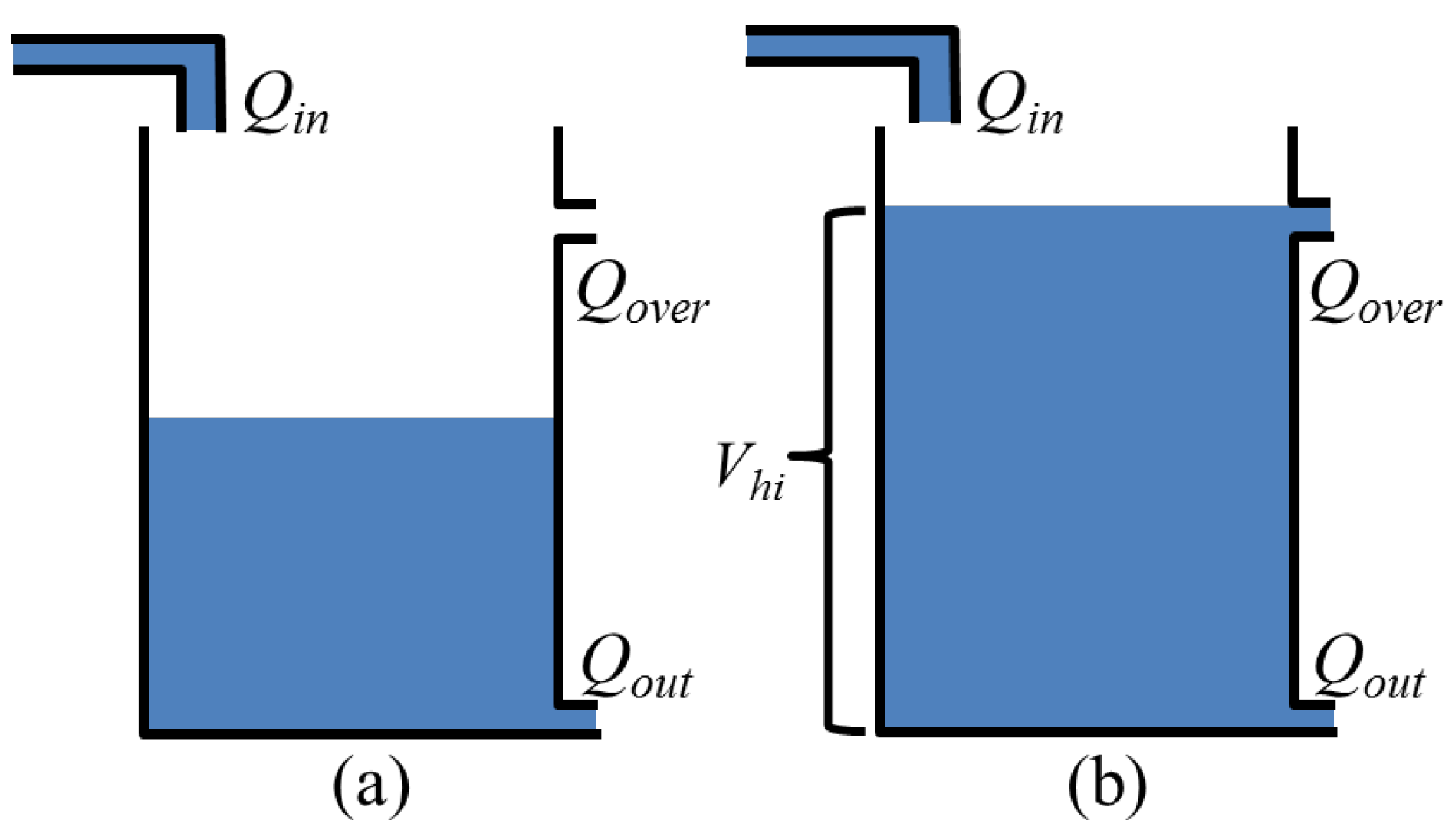
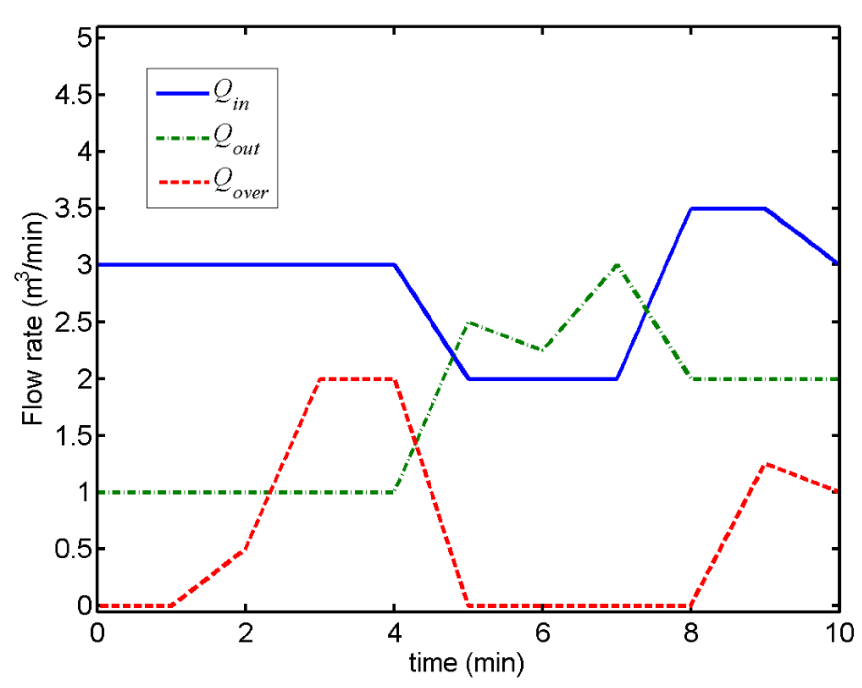
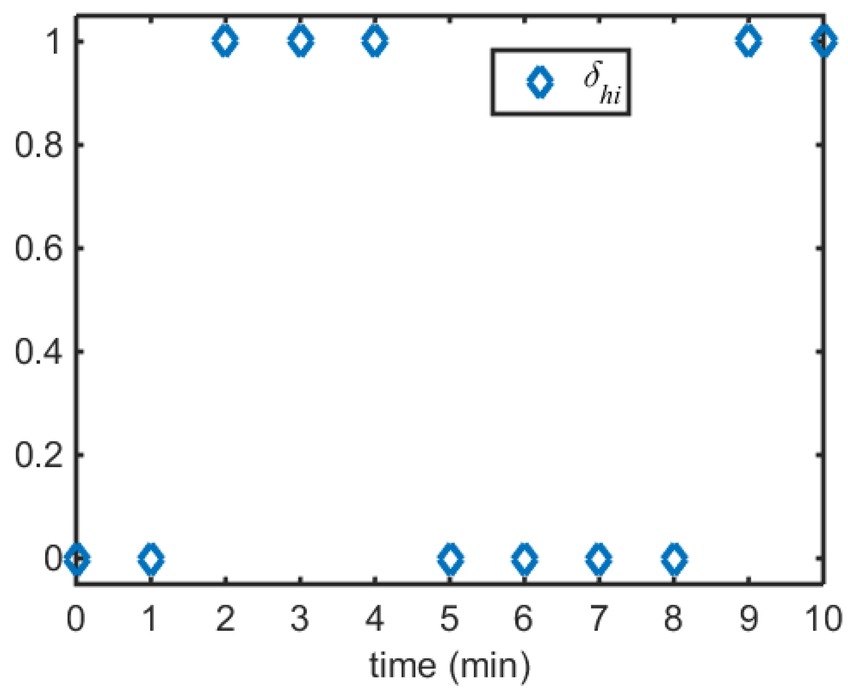
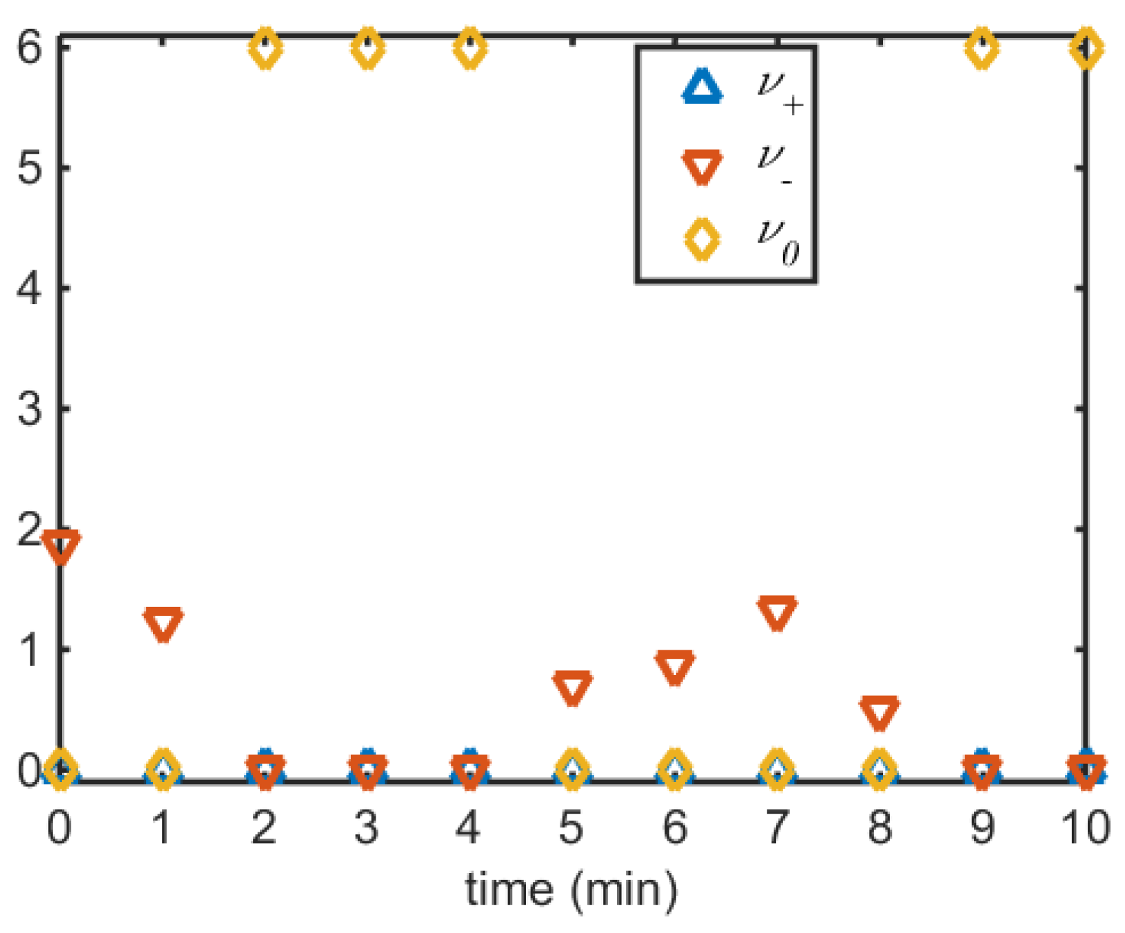
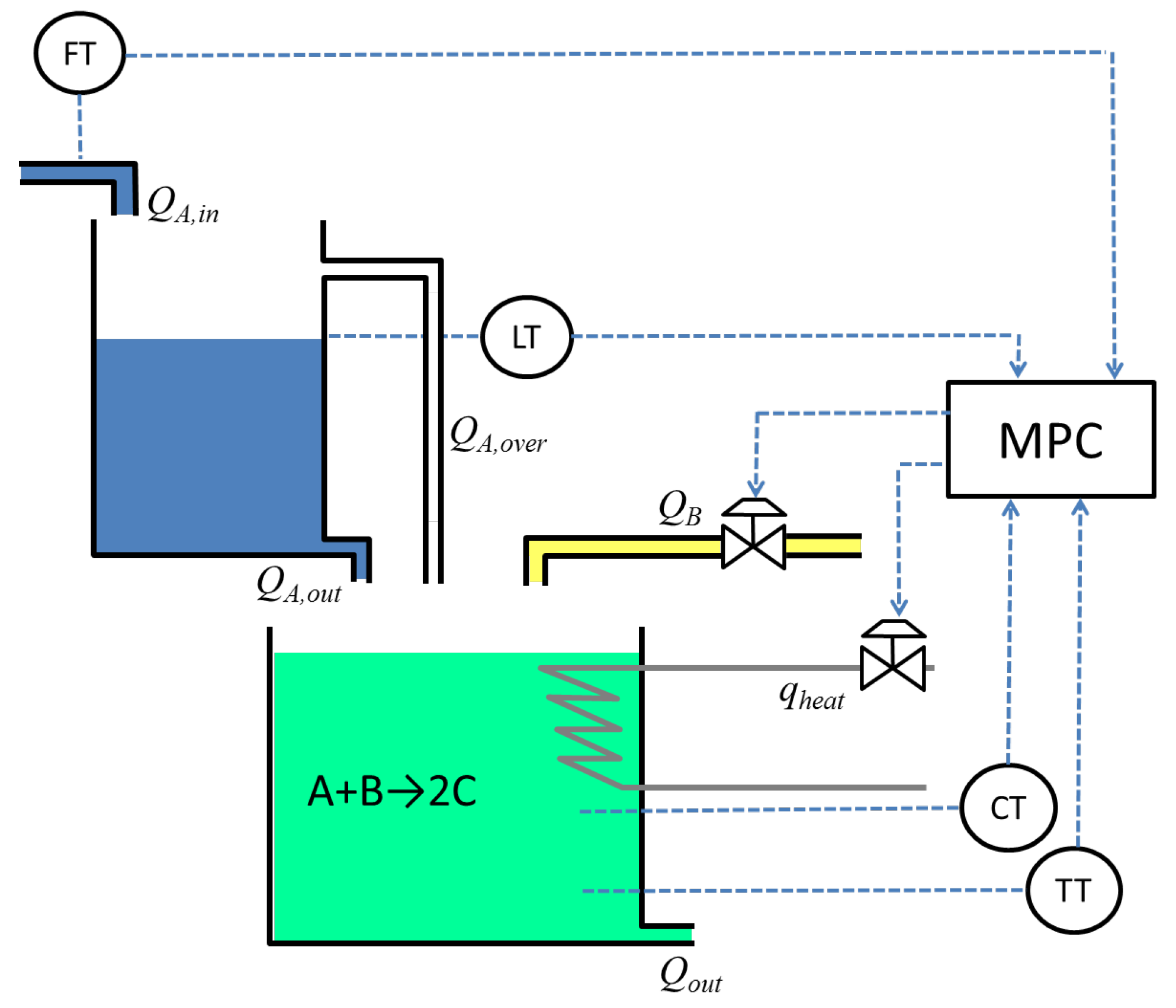
4.1. Tank with Overflow

A simple example to illustrate the need for representing logic in a DAE model is that of a simple tank with overflow, shown in Figure 4.

While the dynamics of this system are trivial, the equations representing the dynamic behavior of the tank change dramatically when the tank reaches the overflow limit. The system, as posed in Equation (28), can be represented as a simple ODE combined with a logical expression determining when the tank overflows:

$$\frac{dV}{dt}=Q_{in}-Q_{out}-Q_{over},$$

(28a)

$$Q_{over}=\left\{\begin{array}{cc}{Q}_{in}-Q_{out}\hfill & \text{if}V\ge V_{max}\&Q_{in}>Q_{out}\hfill \\ 0\hfill & \text{otherwise}\hfill \end{array}\right..$$

(28b)

Here V is the tank volume, $Q_{in}$ is the flow into the tank, $Q_{out}$ is the flow out of the tank, and $Q_{over}$ is the flow exiting the tank as overflow, when the tank volume exceeds the capacity, $V_{max}$. While the system in Equation (28) is very simple, the logical statement Equation (28b) prevents it from being solved using a standard simultaneous solution method. However, by including the algebraic equations representing the Heaviside function MPCC, this system can be solved using a simultaneous solution method. This DAE system translated into a continuous logic formulation using an MPEC with complementarity constraints is given in Equation (29), where Equations (29e)–(29h) represent the additional algebraic equations introduced by the logical MPCC:

$$\frac{dV}{dt}=Q_{in}-Q_{out}-Q_{over},$$

(29a)

$$(1-{\delta }_{hi})Q_{over}=0,$$

(29b)

$$Q_{over}\ge 0,$$

(29c)

$$V\le V_{max},$$

(29d)

$$V-V_{max}={\upsilon }_{+}^2-{\upsilon }_{-}^2,$$

(29e)

$${\upsilon }_{+}{\upsilon }_{-}=0,$$

(29f)

$$\left({\upsilon }_{+}^2+{\upsilon }_{-}^2\right){\upsilon }_0=0,$$

(29g)

$${\upsilon }_{+}^2(1-{\delta }_{hi})+{\upsilon }_{-}^2\left({\delta }_{hi}\right)+{\upsilon }_0(1-{\delta }_{hi})=0.$$

(29h)

In this formulation, ${\delta }_{hi}$ is a pseudo-binary variable that converges to one when the tank is full and zero when it is not full. However, ${\delta }_{hi}$ can have values between one and zero as the solver searches for a solution. When the tank is not full, Equation (29b) will ensure that $Q_{over}$ is zero. When the tank is full, $Q_{over}$ will take on whatever value necessary to satisfy the material balance Equation (29a). However, $Q_{over}$ must be restricted to non-negative values in order to prevent negative values of $Q_{over}$ from satisfying Equation (29a) when the tank is not full. The MPCC tests whether the quantity $V-V_{max}$ is greater than or equal to zero. However, in order to enhance convergence properties, V is also restricted by Equation (29d), so that V cannot exceed the limit. Alternatively, this constraint can be imposed solely by the MPCC equations. However, this may lead to poor convergence properties of the system. Convergence is also enhanced in this case by squaring ${\upsilon }_{+}$ and ${\upsilon }_{-}$ in Equations (29g)–(29h), forcing the squared terms to converge more quickly so that ${\upsilon }_0$ remains near the initial guess in the event that the system is at the volume limit.

To demonstrate the ability of Equation (29) to accurately represent a logic-dependent dynamic system, the set of equations with pre-specified inputs ($Q_{in}$ and $Q_{out}$ , which are shown in Figure 5.) is simulated for 10 minutes. The 10 minute time horizon is discretized into one minute intervals and solved using a simultaneous solution method. This is done using a DAE solution package known as APMonitor [40,41,42]. This software package allows a user to define a model using both differential and algebraic equations [43,44]. The software performs the collocation to convert the differential equations to algebraic equations and the problem is converted to a set of nonlinear algebraic equations. This, and subsequent case studies, use four collocation points in between the discretized time steps in the horizon. See [40] for more details on the APMonitor software. For the optimization example in Section 5, an NLP problem is solved. Because the system is still a continuous set of equations, APMonitor computes the gradient matrices with automatic differentiation, ensuring accuracy and fast solution times. The APOPT solver [45] (which is one of several optional solvers in APMonitor) uses a gradient based, active set optimization algorithm, as opposed to an interior point method such as Interior Point OPTimizer (IPOPT) [46] (which is also one of the optional solvers in APMonitor), and demonstrates good convergence as the problem is solved assuming some set of constraints to be active. This works well with inequality constraints such as Equations (29c)–(29d).

The results of the simulation are shown in Figure 5, Figure 6, Figure 7 and Figure 8. As Figure 5 and Figure 6 illustrate, the overflow ($Q_{over}$) remains at zero until the tank fills.

Once the tank fills, the logical condition that $Q_{over}=0$ is nullified as ${\delta }_{hi}=1$, allowing $Q_{over}$ to take on whatever positive value is needed to satisfy Equation (29a). The complementarity variables (Figure 8) are well behaved, with ${\upsilon }_{-}$ equaling zero when the tank is at the high limit and ${\upsilon }_0$ equaling zero when the tank is not at the high limit. The positive complementarity variable (${\upsilon }_{+}$) is always zero as the system is prevented from exceeding the high limit by Equation (29d). As seen in Figure 8, two of the three complementarity variables must be equal to zero for the formulation to return feasible results. As long as two of the variables are zero, the third variable can take on any positive value.

The results in Figure 5, Figure 6, Figure 7 and Figure 8 illustrate that logic can be embedded into a dynamic system using only continuous algebraic equations to model the system. While convergence for the formulation in Equation (29) is obtained, there are many variations of the MPCC formulation, some of which do not display the same ability to converge consistently. When implementing similarly-formulated MPCCs, it may be necessary to explore various formulations to determine which will be the most robust for the application and choice of solver.

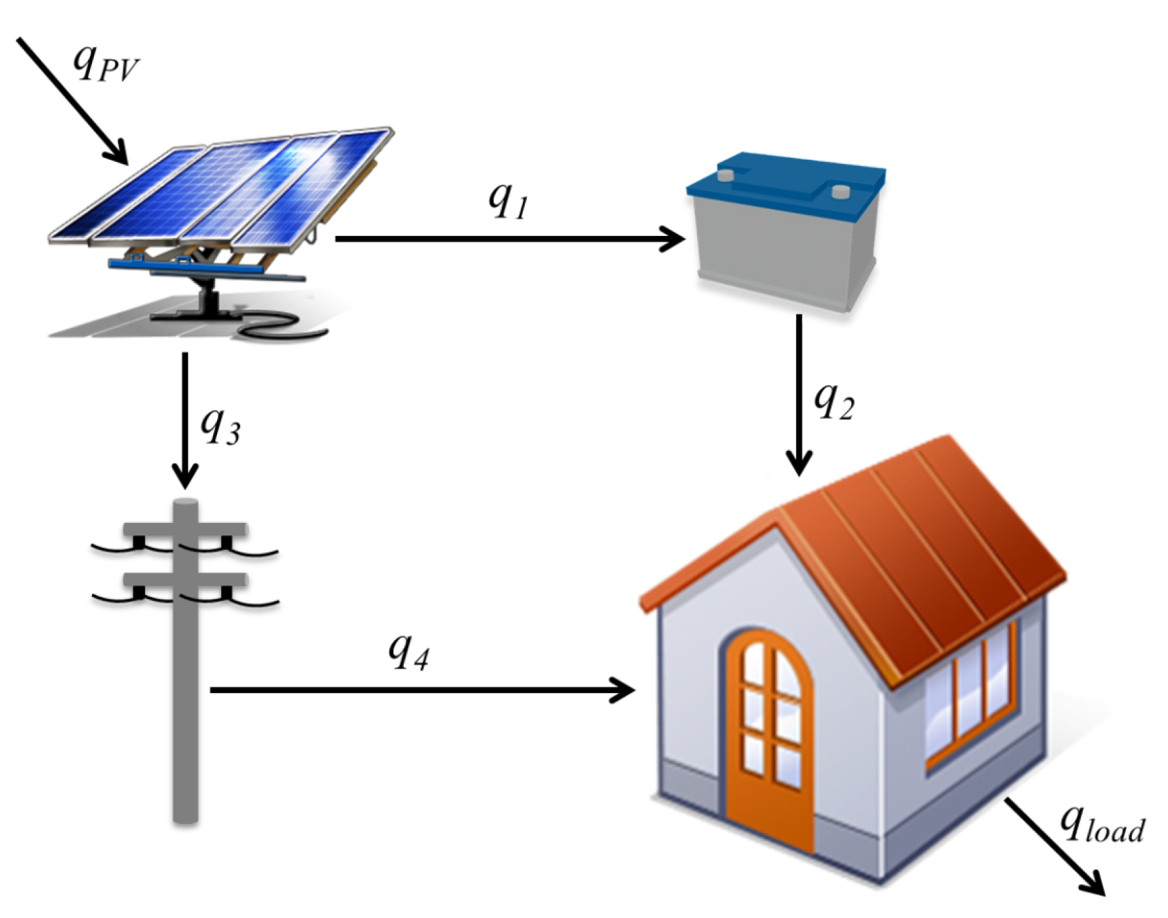
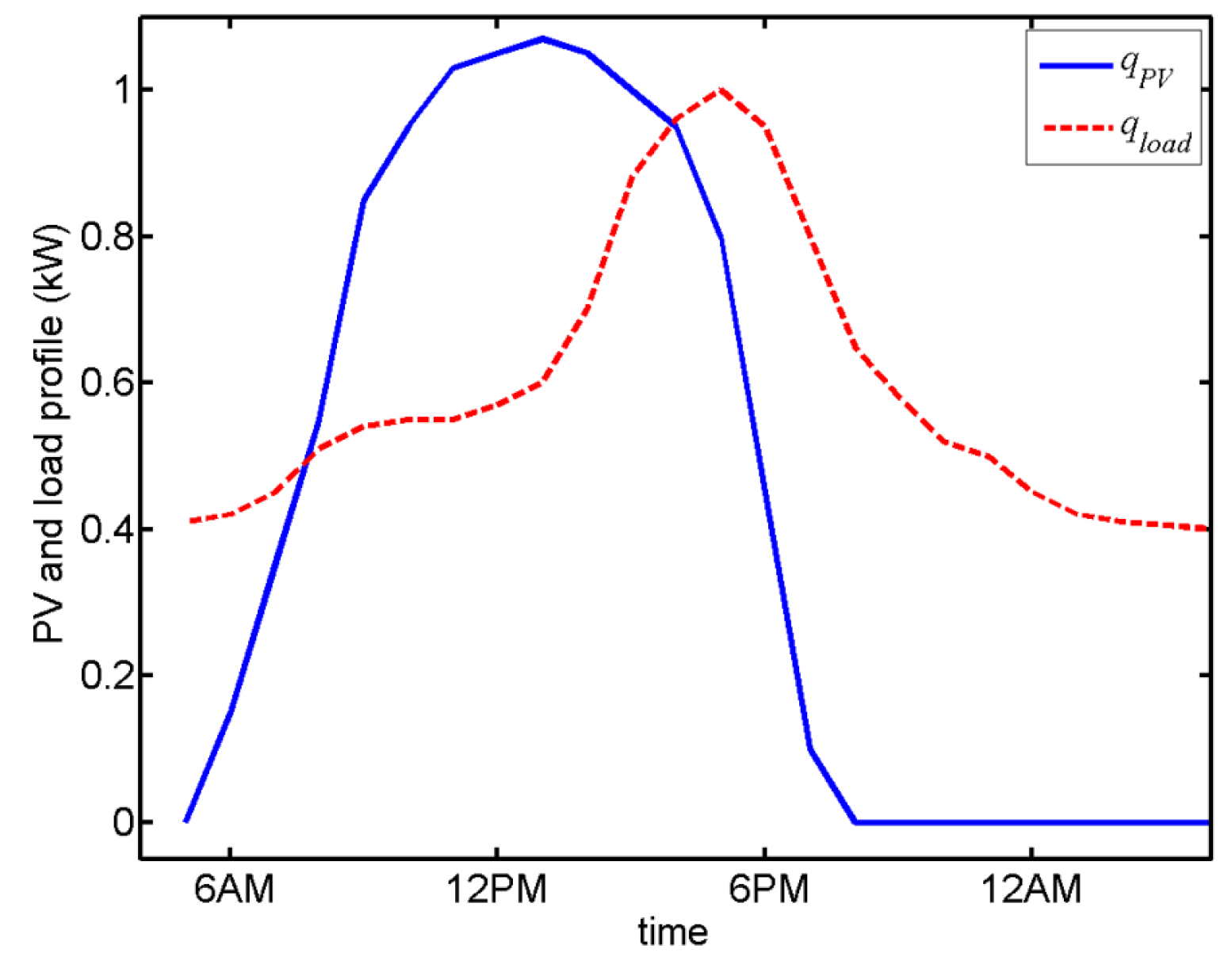
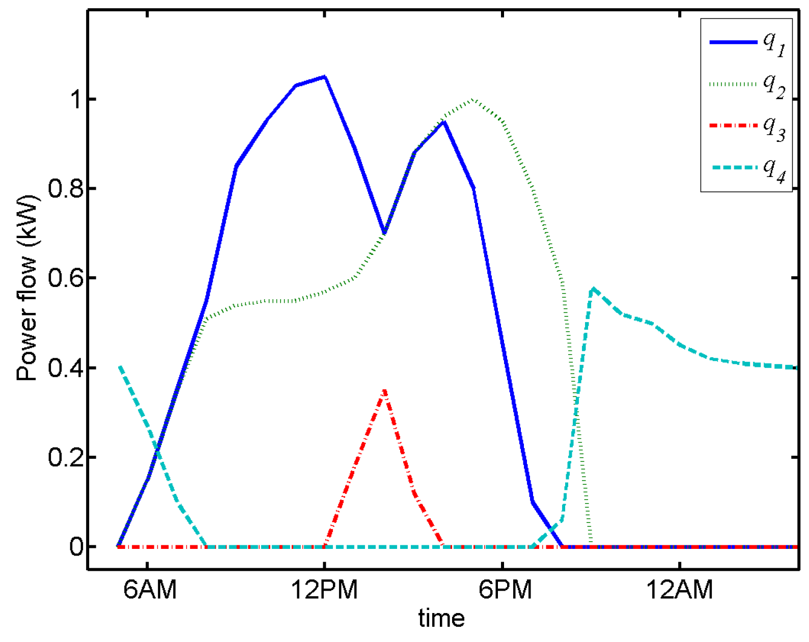
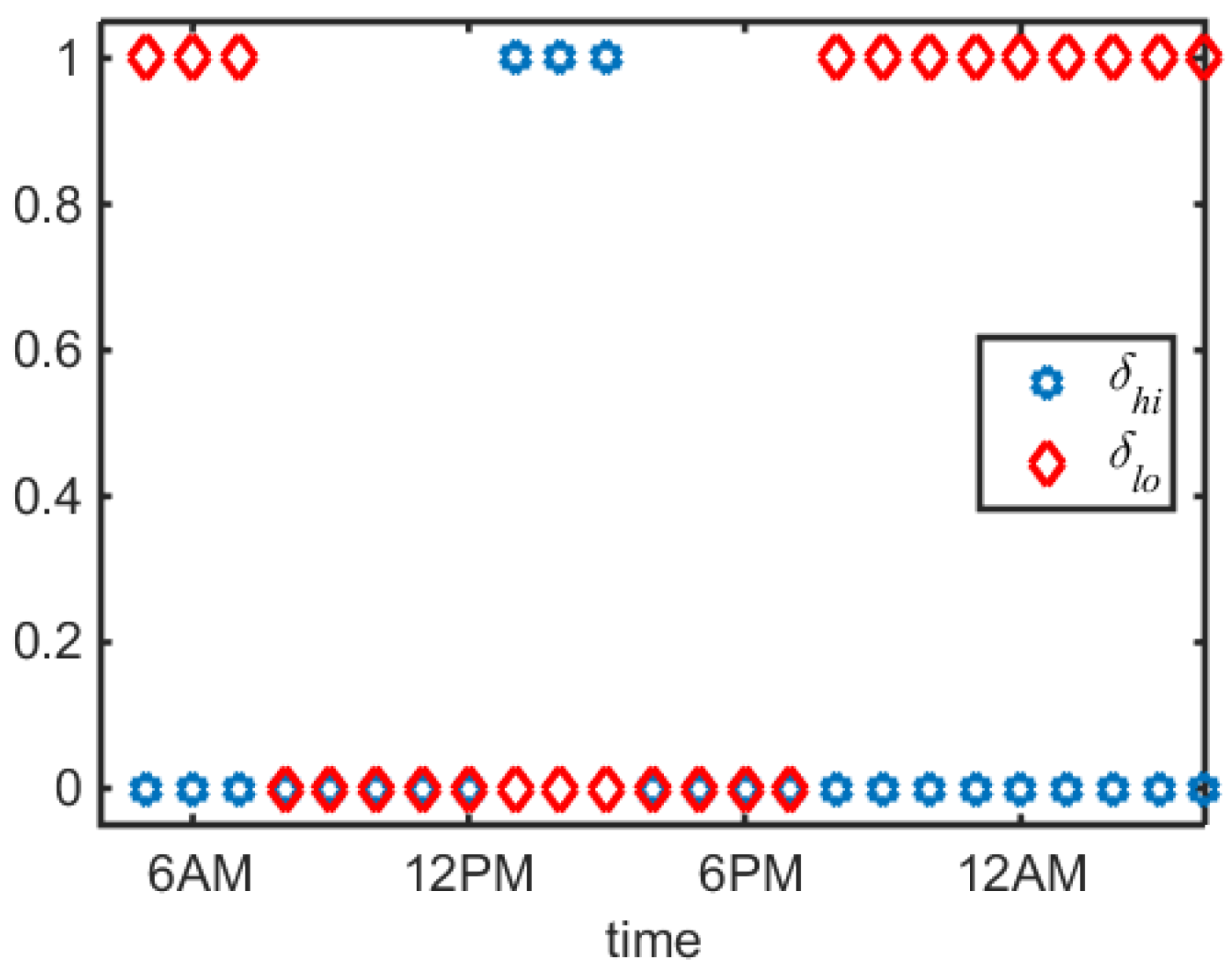
4.2. Power Flow System

The logical MPCC’s performance is also tested in a more complicated simulation of a power flow system (shown in Figure 9) with a photovoltaic solar panel, a battery, a load (represented by a building), and the electric grid. The elements of many energy systems include a combination of multiple energy producers, cyclical energy demand, and energy storage [47,48,49,50,51,52].

This system assumes simple dynamics for the battery Equation (30a). Energy balances are computed around the photovoltaic panel and the load in order to obtain Equations (30b)–(30c), respectively. A logic-based operating strategy is applied in order to specify the system’s operation. Using this strategy, the maximum amount of solar power is delivered to the load by using the battery. When solar power available ($q_{PV}$) exceeds the demand ($q_{load}$), the battery (whose state of charge is represented by $E_{batt}$ and whose initial charge is represented by $E_{batt}^{\circ }$) is charged. When the battery reaches the capacity ($E_{max}$), the excess power is delivered to the grid with flow $q_3$. Conversely, when the battery is void of charge, power must be imported from the grid to the load with flow $q_4$. This logic is specified in Equations (30d)–30e. The variables $q_1$ and $q_2$ represent the power delivered to and extracted from the battery, respectively:

$$\frac{d{E}_{batt}}{dt}=q_1-q_2,$$

(30a)

$$0=q_{PV}-q_1-q_3,$$

(30b)

$$0=q_{load}-q_2-q_4,$$

(30c)

$$q_3=\left\{\begin{array}{cc}{q}_{PV}-q_1\hfill & \text{if}{E}_{batt}\ge E_{max}\&q_{PV}>q_1\hfill \\ 0\hfill & \text{otherwise}\hfill \end{array}\right.,$$

(30d)

$$q_4=\left\{\begin{array}{cc}{q}_{load}-q_2\hfill & \text{if}{E}_{batt}\le 0\&q_{load}>q_2\hfill \\ 0\hfill & \text{otherwise}\hfill \end{array}\right..$$

(30e)

Conversion of the model to continuous form requires two sets of logical MPCC equations representing the logical decisions of Equations 30d–30e. This requires two sets of pseudo-binary (δ) and complementarity variables (υ), which are assigned the subscripts hi and lo, corresponding to the full Equation (30d) and empty Equation (30e) battery charge conditions, respectively. When converted to continuous logic form, Equation (30) becomes Equation (31):

$$E_{batt}^{\circ }=0,$$

(31a)

$$\frac{d{E}_{batt}}{dt}=q_1-q_2,$$

(31b)

$$0=q_{PV}-q_1-q_3,$$

(31c)

$$0=q_{load}-q_2-q_4,$$

(31d)

$$E_{min}\le E_{batt}\le E_{max}.$$

(31e)

High limit MPCC equations corresponding to Equation (30e)

$$(1-{\delta }_{hi})q_3=0,$$

(31f)

$$q_3\ge 0,$$

(31g)

$$E_{max}-E_{batt}={\upsilon }_{hi+}^2-{\upsilon }_{hi-}^2,$$

(31h)

$${\upsilon }_{hi+}{\upsilon }_{hi-}=0,$$

(31i)

$$\left({\upsilon }_{hi+}^2+{\upsilon }_{hi-}^2\right){\upsilon }_{hi,0}=0,$$

(31j)

$${\upsilon }_{hi+}^2(1-{\delta }_{hi})+{\upsilon }_{hi-}^2\left({\delta }_{hi}\right)+{\upsilon }_{hi,0}(1-{\delta }_{hi})=0.$$

(31k)

Low limit MPCC equations corresponding to Equation (30e)

$$(1-{\delta }_{lo})q_4=0,$$

(31l)

$$q_4\ge 0,$$

(31m)

$$E_{min}-E_{batt}={\upsilon }_{lo+}^2-{\upsilon }_{lo-}^2$$

(31n)

$${\upsilon }_{lo+}{\upsilon }_{lo-}=0,$$

(31o)

$$\left({\upsilon }_{lo+}^2+{\upsilon }_{lo-}^2\right){\upsilon }_{lo,0}=0,$$

(31p)

$${\upsilon }_{lo+}^2(1-{\delta }_{lo})+{\upsilon }_{lo-}^2\left({\delta }_{lo}\right)+{\upsilon }_{lo,0}(1-{\delta }_{lo})=0.$$

(31q)

The continuous logic formulation for the power flow system is demonstrated using a simulation with pre-determined $q_{pv}$ and $q_{load}$ over a 24-h time horizon, which is shown in Figure 10.

Hourly time intervals are used in the simulation. As the figure shows, the supply ($q_{pv}$) and demand ($q_{load}$) do not perfectly coincide, with the available solar power peaking near midday and the demand peaking later in the afternoon, requiring the system to use battery energy storage in order to maximize the power delivered to the load from the solar panel. As Figure 11, Figure 12 and Figure 13 illustrate, at the beginning of the day, there is no charge in the battery (indicated by ${\delta }_{lo}=1$) and the demand exceeds the load, forcing power to be drawn from the grid. As the solar power picks up, the battery charges until it reaches the capacity (indicated by ${\delta }_{hi}=1$). When this occurs, the logic dictates that the excess power be exported from the solar panel to the grid, indicated by the positive values for $q_3$ in Figure 11. At the end of the day, the solar power is diminished, the battery completely discharges, and power is again imported from the grid.

The power flow example again demonstrates the value of using MPCCs to represent logical decisions in a DAE system. Embedding this logic in the form of continuous algebraic equations allows the system to be solved using the simultaneous method, which has been proven to significantly increase computational efficiency as compared to a sequential method.

5. Continuous Logic in an NMPC Problem

As a demonstration of the value of integrating logic into a simultaneous solution method, a nonlinear model predictive control (NMPC) problem is solved for a continuous stirred tank reactor (CSTR), which carries out the reaction:

$$A+B⟶2C.$$

(32)

The objective of the controller is to regulate the concentration of component C ($C_C$) using the heat input to the reactor ($q_{heat}$) and the flow rate of component B ($Q_B$) as manipulated variables. The system is subject to disturbances in the flow of component A ($Q_{A,in}$) and is equipped with a surge tank to buffer out the effects of sudden increases in $Q_A$. However, in the case that the volume of fluid in the surge tank exceeds the tank capacity, the surge tank will overflow and a sudden increase in the flow of A will enter the CSTR as shown in Figure 14. NMPC in this scenario can monitor the level in the surge tank (h) and the flow of A coming into the surge tank so that sudden disturbances due to surge tank overflow can be anticipated and accounted for pre-emptively by the controller. The model requires a built-in logical statement as in Equation (28) to represent the tank overflow condition.

In the MPC problem, the outflow from the bottom of the surge tank ($Q_{A,out}$) is proportional to the square root of the height (h) in the tank Equation (34), with the dynamics of the tank represented by a simple material balance Equation (33). The model requires a built-in logical statement to represent the tank overflow condition Equation (35):

$$A_{tank}\frac{dh}{dt}=Q_{A,in}-Q_{A,out}-Q_{A,over},$$

(33)

$$Q_{A,out}=C\sqrt{h},$$

(34)

$$Q_{A,over}=\left\{\begin{array}{cc}{Q}_{A,in}-Q_{A,out}\hfill & \text{if}h\ge h_{max}\&Q_{A,in}>Q_{A,out}\hfill \\ 0\hfill & \text{otherwise}\hfill \end{array}\right..$$

(35)

The CSTR is assumed to be at constant volume so that the total inlet flow equals the flow out ($Q_{out}$) at all times Equation (36):

$$Q_{out}=Q_{A,out}+Q_{A,over}+Q_B.$$

(36)

The kinetics in the CSTR are first order in both A and B and the rate law Equation (37) has temperature dependence subject to the Arrhenius equation, where $R_A$ is the rate of reaction of component A, $k_0$ is the reaction rate constant, $E_A$ is the activation energy, R is the ideal gas constant, T is the temperature in the tank, $C_A$ and $C_B$ are the concentrations of component A and B, respectively:

$$R_A=k_0{e}^{\frac{-E_A}{RT}}{C}_A{C}_B.$$

(37)

The CSTR temperature is determined by an energy balance on the tank Equation (38), where $q_{heat}$ is the rate that heat is delivered to the tank, V is the CSTR volume, ρ and $C_P$ are the density and the heat capacity, respectively of the fluid in the system, and the subscript 0 refers to the fluid before it enters the tank. The components A, B, and C are all assumed dilute so that their concentrations do not affect the density, heat capacity, or overall material balances of the solution. This assumption also permits neglecting heat of reaction in the energy balance:

$$\rho V{C}_P\frac{dT}{dt}=\rho C_P{Q}_{out}\left(T_0-T\right)+q_{heat}.$$

(38)

Material balances on each component are also computed, giving three more differential equations (see Equations (39)–(41)), where $C_C$ is the concentration of component C:

$$V\frac{d{C}_A}{dt}=\left(Q_{A,out}+Q_{A,over}\right)C_{A0}-Q_{out}{C}_A-R_{A}V,$$

(39)

$$V\frac{d{C}_B}{dt}=Q_B{C}_{B0}-Q_{out}{C}_B-R_{A}V,$$

(40)

$$V\frac{d{C}_C}{dt}=2R_{A}V-Q_{out}{C}_C.$$

(41)

The MPC problem seeks to minimize deviations from the setpoint for $C_C$ subject to disturbances in $Q_{A,in}$ without making drastic control moves. To achieve this trade-off, a quadratic performance index is used where the squared deviations at the end of each time interval are weighted differently (10 for setpoint deviations and 1 for manipulated variable changes) and summed to create a performance index to be minimized. This yields the dynamic optimization problem in Equation (42), which is subject to the system model in Equations 33-41 and inequality constraints on the inputs:

$$\begin{array}{cccc}& \underset{Q_B,q_{heat}}{\text{min}}\hfill & & \sum _{i=1}^{N_t}10{\left(C_{C,i}-C_{C,SP}\right)}^2+\sum _{i=1}^{N_t}1{\left(Q_{B,i}-Q_{B,i-1}\right)}^2+\sum _{i=1}^{N_t}1{\left(q_{heat,i}-q_{heat,i-1}\right)}^2.\hfill \\ & \text{Subject}\text{to}\hfill & & \text{Equations}(33)–(41),\hfill \end{array}$$

(42a)

$$0\le Q_B\le Q_{B,max},$$

(42b)

$$0\le q_{heat}\le Q_{heat,max}.$$

(42c)

A first order hold is used for the manipulated variables (MVs) where the value of these variables is held constant over each time interval. A total of $N_t$ time intervals are used in the model prediction. As Figure 14 shows, the controller checks the most recent state measurements (concentrations and temperature in the CSTR and fluid height in the surge tank) and disturbance measurements (flow of A) at each time step in order to update the model and ensure accurate future predictions. The model with built-in logic for surge tank overflow allows the controller to anticipate large influxes of flow and proactively account for this disturbance.

The optimization problem posed in Equation (42) is solved using both a sequential and a simultaneous solution method. In this problem, $N_t=30$ over 1 min time intervals with a control horizon equal to the prediction horizon of 50 min. With two MVs, the optimization problem has 100 degrees of freedom in total. The sequential method version of the problem uses an optimization solver (FMINCON) in MATLAB [53], which takes pre-determined values of the inputs, simulates the system using an explicit ODE integrator (ODE45), computes the objective function and uses this information to construct numeric approximations to the gradient matrices to compute a new search direction for the next iteration. The sequential method also uses if/then logic as in Equation (28b) to describe the changing dynamics of the surge tank. This methodology requires simulating through the entire time horizon of the system model thousands of times in order to generate the gradient matrices and iterate.

The simultaneous version of the problem is solved using APMonitor with the Heaviside function MPCC described in Equation (29), which, uses the orthogonal collocation scheme described in Section 4.1. This allows the problem to be expressed entirely as a set of algebraic equations and inequality constraints, which can be solved using NLP methods. The APOPT solver is again used to obtain a solution to this NLP problem. This method does not require multiple simulations of the system model as it solves the constraints of the system simultaneously subject to minimization of the objective function. As opposed to the sequential approach, the simultaneous method converges the equation residuals only once at the optimal solution. It should be noted that other methods do exist for approaching discontinuities in dynamic problems, such as a multiple shooting method, which is somewhat of a hybrid of the two methodologies shown here. The comparison in this NMPC problem is intended to demonstrate that the simultaneous solution method with MPECs to represent logical constraints in the system is a viable method for this particular problem by comparison to a purely sequential method with explicit if/then logic to represent disjunctions that arise over the course of the dynamic simulation.

The MPC problem is solved with the system initially at steady state with $Q_{A,in}=Q_{B,in}=0.5{\text{m}}^3/\text{min}$ and $C_C$ exactly on setpoint at $3{\text{mol/m}}^3$. At time $t=0$, however, a step change disturbance is introduced, changing $Q_{A,in}$ to $0.8{\text{m}}^3/\text{min}$. The results from each solution method showing the controlled variable (CV) and the MVs are shown in Figure 15.

As the figure shows, despite the introduction of a large disturbance, the CV is maintained very near the setpoint in each case. There is little difference in objective function values (1%) when comparing the two methods. The differences may be attributed to choice of solvers (APOPT for simultaneous versus FMINCON for sequential), automatic differentiation (simultaneous) versus finite differences (sequential) for gradients, or differences in discretization with collocation (simultaneous) versus an adaptive step integrator (sequential). For these reasons and others, the two methods arrive at slightly different solutions. Computationally, the sequential method converged with 51 iterations (in 883 sec) with $5,292$ model trajectory solutions that required $16,393,388$ model derivative evaluations. The number of model intermediate solutions and computational time would significantly decrease if exact sensititivities were computed [54] versus the finite difference approach used in this study to obtain gradients. The simultaneous method completed with 87 iterations (in $5.2$ sec) and had $46,500$ model residual evaluations and $17,400$ gradient evaluations. All computational times are with an Intel i7-2760QM CPU operating at 2.4 GHz with 8 GB RAM.

The profiles of some relevant state variables are shown in Figure 16 for the simultaneous solution method. As these plots indicate, the continuous logic formulation produces the desired switching behavior.

As the surge tank reaches the overflow condition, the tank overflows but otherwise, $Q_{A,over}=0$. In this MPC application, it is invaluable to have the overflow condition represented in the model, as it allows the controller to anticipate large interruptions to the operation of the CSTR. While the disturbance it introduced at $t=0$, the major impact is not observed until $t=18$ min when the tank overflows. The model, however, allows for this change to be predicted and control moves to be made pre-emptively. As Figure 15 shows, more drastic control moves are made several minutes before the tank overflows. Predicting this occurrence with a logic-embedded model allows the system to effectively maintain the setpoint despite the large change in operating conditions.

6. Conclusions

This work demonstrates how logical expressions based on the Heaviside function can be used in NMPC and simulation while still taking advantage of the benefits of simultaneous solution methods. The equations, known as MPCCs, can be embedded into a DAE model using continuous algebraic equations. The MPCCs take advantage of complementarity conditions, requiring that an equality and an inequality constraint be active at all times. The major limitation of this MPCC formulation is its inherent ambiguity when $x=0$. This inherent limitation makes the significance of this formulation reliant on solver convergence properties and subject to simultaneous solution method initialization challenges. Two simulation examples have been presented to demonstrate the viability of using MPCCs to represent these logical decisions. The examples, as presented, demonstrate rapid and accurate convergence, illustrating how a logical operating scheme can be simulated using an efficient simultaneous solution method.

In addition to simulation, an NMPC problem is also solved using the formulation developed in this work. The simultaneous solution method combined with the continuous logic formulation is compared to a sequential method using simple if/then logic. The results show that each of the the methods produce adequate solutions. The simultaneous method with continuous logic is faster in obtaining a solution, but a more sophisticated implementation of the sequential method would likely yield comparible solutions times. The continuous logic formulation allows implementation of logical statements into a model without having to use the less efficient sequential method for real-time NMPC or dynamic optimization calculations. The model including the dynamics and the logical statements are implemented as a continuous system of algebraic equations, which can be solved with efficient NLP solvers.

While the examples posed in this work demonstrate the potential of using MPCCs for logical decisions, this nascent topic requires much more research to be a viable method for solving optimization problems with such decisions. One of the key challenges to overcome is the non-convexity that is characteristic of many problems with logical decisions, which can cause issues with convergence due to hidden non-smoothness in the formulation or ill conditioning. Furthermore, future work on this formulation must include a study of the mathematical properties of logical MPCCs to provide a better understanding of how these problems are handled by various solvers and what can be done to further enhance performance. In particular, in the examples in this paper, the logical conditions are dependent on pre-determined inputs. Optimality is more difficult to obtain when the logical statements depend on the decision variables, with the optimizer typically finding a feasible solution and stopping. This issue is one that requires further understanding of how a solver deals with logic dependent on decision variables. This paper presents the concept of using MPCCs to represent logical decisions when using a simultaneous solution method so that this concept may be explored for other applications.

References

1. Trespalacios, F.; Grossmann, I.E. Algorithmic Approach for Improved Mixed-Integer Reformulations of Convex Generalized Disjunctive Programs. INFORMS J. Comput. 2015, 27, 59–74. [Google Scholar] [CrossRef]
2. Movahedian, N.; Nobakhtian, S. Necessary and sufficient conditions for nonsmooth mathematical programs with equilibrium constraints. Nonlinear Anal. Theory Methods Appl. 2010, 72, 2694–2705. [Google Scholar] [CrossRef]
3. Yin, H.; Ding, F.; Zhang, J. Active set algorithm for mathematical programs with linear complementarity constraints. Appl. Math. Comput. 2011, 217, 8291–8302. [Google Scholar] [CrossRef]
4. Tangaramvong, S.; Tin-Loi, F. An FE-MPEC approach for limit load evaluation in the presence of contact and displacement constraints. Int. J. Solids Struct. 2012, 49, 1753–1763. [Google Scholar] [CrossRef]
5. Tangaramvong, S.; Tin-Loi, F.; Senjuntichai, T. An MPEC approach for the critical post-collapse behavior of rigid-plastic structures. Int. J. Solids Struct. 2011, 48, 2732–2742. [Google Scholar] [CrossRef]
6. Baumrucker, B.; Renfro, J.; Biegler, L.T. MPEC problem formulations and solution strategies with chemical engineering applications. Comput. Chem. Eng. 2008, 32, 2903–2913. [Google Scholar] [CrossRef]
7. Raghunathan, A.U.; Biegler, L.T. Mathematical programs with equilibrium constraints (MPECs) in process engineering. Comput. Chem. Eng. 2003, 27, 1381–1392. [Google Scholar] [CrossRef]
8. Raghunathan, A.U.; Diaz, M.S.; Biegler, L.T. An MPEC formulation for dynamic optimization of distillation operations. Comput. Chem. Eng. 2004, 28, 2037–2052. [Google Scholar] [CrossRef]
9. Zhou, L.; Liao, Z.; Wang, J.; Jiang, B.; Yang, Y.; Du, W. Energy configuration and operation optimization of refinery fuel gas networks. Appl. Energy 2015, 139, 365–375. [Google Scholar] [CrossRef]
10. Gabriel, S.A.; Leuthold, F.U. Solving discretely-constrained MPEC problems with applications in electric power markets. Energy Econ. 2010, 32, 3–14. [Google Scholar] [CrossRef]
11. Chen, Y.H.H.; Paltsev, S.; Reilly, J.M.; Morris, J.F.; Babiker, M.H. Long-term economic modeling for climate change assessment. Econ. Model. 2016, 52, 867–883. [Google Scholar] [CrossRef]
12. Walpen, J.; Mancinelli, E.; Lotito, P. A heuristic for the OD matrix adjustment problem in a congested transport network. Eur. J. Oper. Res. 2015, 242, 807–819. [Google Scholar] [CrossRef]
13. Kovacevic, R.; Pflug, G. Electricity swing option pricing by stochastic bilevel optimization: A survey and new approaches. Eur. J. Oper. Res. 2014, 237, 389–403. [Google Scholar] [CrossRef]
14. Júdice, J. Optimization with linear complementarity constraints. Pesquisa Oper. 2014, 34, 559–584. [Google Scholar] [CrossRef]
15. Baumrucker, B.; Biegler, L. MPEC strategies for optimization of a class of hybrid dynamic systems. J. Process Control 2009, 19, 1248–1256. [Google Scholar] [CrossRef]
16. Baumrucker, B.; Biegler, L.T. MPEC strategies for cost optimization of pipeline operations. Comput. Chem. Eng. 2010, 34, 900–913. [Google Scholar] [CrossRef]
17. Hedengren, J.D. MPEC: Mathematical Programs with Equilibrium Constraints. Available online: http://apmonitor.com/wiki/index.php/Apps/MpecExamples (Accessed on 31 December 2015).
18. Björkqvist, J.; Westerlund, T. Automated reformulation of disjunctive constraints in MINLP optimization. Comput. Chem. Eng. 1999, 23, S11–S14. [Google Scholar] [CrossRef]
19. Grossmann, I.E. Review of nonlinear mixed-integer and disjunctive programming techniques. Optim. Eng. 2002, 3, 227–252. [Google Scholar] [CrossRef]
20. Belotti, P.; Kirches, C.; Leyffer, S.; Linderoth, J.; Luedtke, J.; Mahajan, A. Mixed-integer nonlinear optimization. Acta Numer. 2013, 22, 1–131. [Google Scholar] [CrossRef]
21. Grossmann, I.E.; Türkay, M. Solution of algebraic systems of disjunctive equations. Comput. Chem. Eng. 1996, 20, S339–S344. [Google Scholar] [CrossRef]
22. Liu, G.; Zhang, J. A new branch and bound algorithm for solving quadratic programs with linear complementarity constraints. J. Comput. Appl. Math. 2002, 146, 77–87. [Google Scholar] [CrossRef]
23. Sawaya, N.W.; Grossmann, I.E. A cutting plane method for solving linear generalized disjunctive programming problems. Comput. Chem. Eng. 2005, 29, 1891–1913. [Google Scholar] [CrossRef]
24. Andreani, R.; Júdice, J.J.; Martínez, J.M.; Martini, T. Feasibility Problems with Complementarity Contraints. Eur. J. Oper. Res. 2016, 249, 41–54. [Google Scholar] [CrossRef]
25. Biegler, L.T. An overview of simultaneous strategies for dynamic optimization. Chem. Eng. Process.: Process Int. 2007, 46, 1043–1053. [Google Scholar] [CrossRef]
26. Diehl, M.; Ferreau, H.J.; Haverbeke, N. Nonlinear Model Predictive Control: Towards New Challenging Applications; Springer Berlin Heidelberg: Berlin, Heidelberg, Germany, 2009; Chapter Efficient Numerical Methods for Nonlinear MPC and Moving Horizon Estimation; pp. 391–417. [Google Scholar]
27. Bertsekas, D.P. Dynamic Programming and Suboptimal Control: A Survey from ADP to MPC. Eur. J. Control 2005, 11, 310–334. [Google Scholar] [CrossRef]
28. Su, J.; Renaud, J. Automatic Differentiation in Robust Optimization. AIAA J. 1997, 35, 1072–1079. [Google Scholar] [CrossRef]
29. Tanartkit, P.; Biegler, L.T. Stable decomposition for dynamic optimization. Ind. Eng. Chem. Res. 1995, 34, 1253–1266. [Google Scholar] [CrossRef]
30. Hedengren, J.D.; Allsford, K.V.; Ramlal, J. Moving horizon estimation and control for an industrial gas phase polymerization reactor. In Proceedings of the IEEE American Control Conference (ACC’07), Marriott Marquis Hotel at Times Square, New York City, NY, USA, 11–13 July 2007; pp. 1353–1358.
31. Leibman, M.; Edgar, T.; Lasdon, L. Efficient data reconciliation and estimation for dynamic processes using nonlinear programming techniques. Comput. Chem. Eng. 1992, 16, 963–986. [Google Scholar] [CrossRef]
32. Spivey, B.J.; Hedengren, J.D.; Edgar, T.F. Constrained nonlinear estimation for industrial process fouling. Ind. Eng. Chem. Res. 2010, 49, 7824–7831. [Google Scholar] [CrossRef]
33. Carey, G.; Finlayson, B.A. Orthogonal collocation on finite elements. Chem. Eng. Sci. 1975, 30, 587–596. [Google Scholar] [CrossRef]
34. Finlayson, B.A. Orthogonal collocation on finite elements-progress and potential. Math. Comput. Simul. 1980, 22, 11–17. [Google Scholar] [CrossRef]
35. Bequette, B.W. Nonlinear control of chemical processes: A review. Ind. Eng. Chem. Res. 1991, 30, 1391–1413. [Google Scholar] [CrossRef]
36. Zavala, V.M. Computational Strategies for the Optimal Operation of Large-Scale Chemical Processes. PhD dissertation, Carnegie Mellon University, 2008. [Google Scholar]
37. Biegler, L.T.; Cervantes, A.M.; Wächter, A. Advances in simultaneous strategies for dynamic process optimization. Chem. Eng. Sci. 2002, 57, 575–593. [Google Scholar] [CrossRef]
38. Hughes, T.J.; Reali, A.; Sangalli, G. Efficient quadrature for NURBS-based isogeometric analysis. Comput. Methods Appl. Mech. Eng. 2010, 199, 301–313. [Google Scholar] [CrossRef]
39. Safdarnejad, S.M.; Hedengren, J.D.; Lewis, N.R.; Haseltine, E.L. Initialization strategies for optimization of dynamic systems. Comput. Chem. Eng. 2015, 78, 39–50. [Google Scholar] [CrossRef]
40. Hedengren, J.D.; Shishavan, R.A.; Powell, K.M.; Edgar, T.F. Nonlinear modeling, estimation and predictive control in APMonitor. Comput. Chem. Eng. 2014, 70, 133–148. [Google Scholar] [CrossRef]
41. Spivey, B.; Hedengren, J.; Edgar, T. Constrained Control and Optimization of Tubular Solid Oxide Fuel Cells for Extending Cell Lifetime. In Proceedings of the American Control Conference (ACC’12), Fairmont Queen Elizabeth Hotel, Montreal, QC, Canada, 27–29 June 2012; pp. 1356–1361.
42. Jacobsen, L.; Spivey, B.; Hedengren, J. Model Predictive Control with a Rigorous Model of a Solid Oxide Fuel Cell. In Proceedings of the American Control Conference (ACC’13), Renaissance Downtown Hotel, Washington, DC, USA, 17–19 June 2013; pp. 3747–3752.
43. Hedengren, J. APMonitor Modeling Language for Mixed-Integer Differential Algebraic Systems. In Proceedings of the Computing Society Session on Optimization Modeling Software: Design and Applications, INFORMS National Meeting, Phoenix Convention Center, Phoenix, AZ, USA, 14–17 October 2012.
44. Hedengren, J.D.; Eaton, A.N. Overview of Estimation Methods for Industrial Dynamic Systems. Optim. Eng. 2015. [Google Scholar] [CrossRef]
45. Hedengren, J.; Mojica, J.; Cole, W.; Edgar, T. APOPT: MINLP Solver for Differential and Algebraic Systems with Benchmark Testing. In Proceedings of the INFORMS National Meeting, Phoenix Convention Center, Phoenix, AZ, USA, 14–17 October 2012.
46. Wächter, A.; Biegler, L.T. On the implementation of an interior-point filter line-search algorithm for large-scale nonlinear programming. Math. Program. 2006, 106, 25–57. [Google Scholar] [CrossRef]
47. Powell, K.M.; Sriprasad, A.; Cole, W.J.; Edgar, T.F. Heating, cooling, and electrical load forecasting for a large-scale district energy system. Energy 2014, 74, 877–885. [Google Scholar] [CrossRef]
48. Powell, K.M.; Cole, W.J.; Ekarika, U.F.; Edgar, T.F. Optimal chiller loading in a district cooling system with thermal energy storage. Energy 2013, 50, 445–453. [Google Scholar] [CrossRef]
49. Powell, K.M.; Edgar, T.F. Modeling and control of a solar thermal power plant with thermal energy storage. Chem. Eng. Sci. 2012, 71, 138–145. [Google Scholar] [CrossRef]
50. Cole, W.J.; Powell, K.M.; Edgar, T.F. Optimization and advanced control of thermal energy storage systems. Energy Build. 2012, 28, 81–99. [Google Scholar] [CrossRef]
51. Powell, K.; Hedengren, J.; Edgar, T. Dynamic Optimization of a Solar Thermal Energy Storage System over a 24 Hour Period using Weather Forecasts. In Proceedings of the American Control Conference (ACC’13), Renaissance Downtown Hotel, Washington, DC, USA, 17–19 June 2013; pp. 2952–2957.
52. Powell, K.M.; Hedengren, J.D.; Edgar, T.F. Dynamic optimization of a hybrid solar thermal and fossil fuel system. Solar Energy 2014, 108, 210–218. [Google Scholar] [CrossRef]
53. MATLAB. Version 8.5.0 (R2015a), The MathWorks Inc.: Natick, MA, USA, 2015.
54. Lewis, N.R.; Hedengren, J.D.; Haseltine, E.L. Hybrid Dynamic Optimization Methods for Systems Biology with Efficient Sensitivities. Processes 2015, 3, 701–729. [Google Scholar] [CrossRef]
Figure 1. A schematic illustrating the orthogonal collocation on finite elements discretization with a first-order hold assumed for inputs (u) in each element (k). The differential state variables (x) are approximated at each of the collocation points, denoted by i. The points are represented using different shapes and colors, which help distinguish one finite element from another.
Processes 04 00007 g001
Figure 2. A plot showing the convergence of the Heaviside function MPCC when x = 0 . As the plot shows, δ converges to 1 as desired.
Processes 04 00007 g002
Figure 3. A plot of residuals when solving Equation (27) using Newton’s Method when x = 0 .
Processes 04 00007 g003
Figure 4. A schematic showing how the dynamic equations representing a simple tank change when the tank overflows. (a) is with no overflow; and (b) is when there is overflow.
Processes 04 00007 g004
Figure 5. Flow rates in and out of the tank overflow system. Q i n and Q o u t are the model inputs. Q o v e r is a dependent variable, subject to the logical condition of the tank being at the overflow limit.
Processes 04 00007 g005
Figure 6. Tank volume with a high limit ( V m a x ) of 10 m 3 . If the tank volume reaches this limit, overflow may ensue.
Processes 04 00007 g006
Figure 7. The pseudo-binary variable, δ h i , which is a continuous variable that takes on values of 1 (tank full) and 0 (tank empty) at the solution.
Processes 04 00007 g007
Figure 8. Complementarity variables used in the tank overflow system.
Processes 04 00007 g008
Figure 9. Schematic for the power flow example with photovoltaic panel, battery, electric grid, and a load (represented by the building) with the corresponding flows defined between these elements.
Processes 04 00007 g009
Figure 10. Inputs to the power flow model with q p v (the electric power flow entering the photovoltaic panel) and q l o a d (the power demand of the building).
Processes 04 00007 g010
Figure 11. Flows in the power network illustrating the viability of the continuous logic MPCC formulation.
Processes 04 00007 g011
Figure 12. State of charge (kWh) of the battery with an upper limit of 2 kWh.
Processes 04 00007 g012
Figure 13. Pseudo-binary variables indicating a fully charged battery ( δ h i ) and a fully discharged battery ( δ l o ).
Processes 04 00007 g013
Figure 14. A schematic showing the MPC scheme of a CSTR and surge tank with overflow.
Processes 04 00007 g014
Figure 15. Results from the CSTR with surge tank nonlinear MPC problem showing the solution from the sequential method (blue solid line) with the simultaneous method (red dashed line), where C C is the controlled variable with a setpoint change from 3 to 4 mol/m 3 (a), Q B and q h e a t are manipulated variables subject to a zero-order hold.
Processes 04 00007 g015
Figure 16. Results of the CSTR MPC problem showing other differential and algebraic state variables with time including the compositions of A and B (a); height of fluid in the surge tank (b); and flow from the surge tank (c).
Processes 04 00007 g016