Fault Classification Decision Fusion System Based on Combination Weights and an Improved Voting Method

Abstract

It is difficult to correctly classify all faults by using only one classifier, and the performance of most classifiers varies under different conditions. In view of this, a new decision fusion system is proposed to solve the problem of fault classification. The proposed decision fusion system is innovative in two aspects: the use of combined weights and a new improved voting method. The combined weights integrate the subjective and objective weights, where the analytic hierarchy process and entropy weight-technique for order performance by similarity to ideal solution are used to determine the subjective and objective weights of different base classifiers under multiple performance evaluation indicators. Moreover, a new improved voting method based on the concept of classifier validity is proposed to increase the accuracy of the decision system. Finally, the method is validated by the Tennessee Eastman benchmark process, and the classification accuracy of the new method is shown to be improved by more than 5.06% compared to the best base classifier.

1. Introduction

With the development of technology and social progress, industrialization and automation have occupied increasingly important positions in industrial production. Safety production is one of the key principles of industrial production, and fault diagnosis is an effective means to ensure safe production. It is important to classify various faults in a timely and accurate manner during the fault diagnosis process.

Data-driven fault diagnosis methods are often used for fault classification. They use artificial intelligence technology to build a model from the historical data for fault classification [1]. There are many reported results on the specific content of data-driven fault diagnosis methods [2,3,4].

However, any fault classification method has its limitations and often cannot classify all faults correctly. Hence, a concept that integrates various classification methods to classify the same object has gradually been accepted [5,6]. Based on an effective ensemble method, the decision fusion system often provides more accurate classification results.

The performance of an ensemble classification system is mainly affected by two factors, namely the diversity of the base classifiers and the decision fusion strategy. The latter is studied in this paper. The role of the decision fusion strategy is to combine the decisions of various base classifiers to enhance the final classification results and reduce decision conflicts. The effectiveness of the decision fusion theory had been verified in many studies [7,8,9]. Basic decision fusion strategies include the voting method, the weighted voting method, Bayesian theory, and the Dempster–Shafer evidence theory [10,11,12,13]. Of these, the voting method is a simple and useful fusion strategy, but it treats all base classifiers equally, which is inappropriate.

In fact, the performance of each base classifier varies under different conditions. It is necessary to evaluate the performance of the base classifier and determine the weight or priority of the base classifiers according to specific conditions. This has rarely been studied in the field of fault classification [14,15]. In addition, there are many performance evaluation indicators for the base classifier, and a single performance evaluation indicator cannot comprehensively measure the performance of the base classifier. In view of this, Ge et al. [14,15] pointed out that multiple evaluation indicators can provide more detailed information about the base classifiers, which is more conducive to the determination of the weights for the base classifiers. Additionally, they proposed to determine the weight of the base classifier by the analytic hierarchy process (AHP) under multiple evaluation indicators in [14,15].

The AHP can be combined with expert experience to generate the subjective weights of the base classifiers. However, it is unreliable to consider only subjective weights in a decision system. When the subjective tendency of the expert is serious, mistakes will inevitably occur. On the contrary, the objective weight relies entirely on the data and is not affected by personal preferences. However, counter-intuitive results may appear if the weights are determined only from the data. Therefore, a natural idea is to combine the subjective weight with the objective weight to obtain the combined weight (CW).

In this paper, a new decision fusion system based on the CW and an improved voting method is proposed. In the proposed decision fusion system, the CW, which integrates the subjective and objective weights is determined using the AHP and EW-TOPSIS (entropy weight-technique for order performance by similarity to ideal solution). In addition, a new improved voting method is proposed based on the concept of validity, which is used to distinguish the performance differences of different fault classification methods for different faults. Thus, the rigid 0–1 rule of the voting method can be avoided, and the advantages of various base classifiers for different faults can be maximized. The proposed decision fusion system is illustrated in the Tennessee Eastman (TE) benchmark process.

The rest of the paper is organized as follows. Section 2 reviews the AHP and EW-TOPSIS. Section 3 describes the proposed method. In Section 4, the performance of the proposed decision fusion system is verified by the TE process. Finally, conclusions are made.

2. Methods

2.1. The AHP

The AHP was originally introduced by Saaty to determine the best scheme based on experience [16]. It can concretize the subjective judgments and tendencies of experts and express them in numerical form to determine the priority levels of alternatives. There are usually three levels for the simplest AHP, namely the topmost target layer, the middle standard layer, and the bottom-most alternative layer. The middle standard layer can be further subdivided, and substandard layers can be established to obtain a more comprehensive and detailed judgment indicator for some more complex or accurate problems. Assuming there are n indicators and m alternatives, the specific steps of the AHP are described as follows [17,18,19,20,21]:

Step 1: Determine the hierarchy structure according to actual problems and needs.

Step 2: Construct the judgment matrix according to expert experience.

$$A=\left[\begin{array}{ccc}{a}_{11}& \cdots & a_{1n}\\ ⋮& \ddots & ⋮\\ a_{n1}& \cdots & a_{nn}\end{array}\right]$$

(1)

where $a_{ij}$ represents the importance of indicator i compared to indicator j; $a_{ji}=1/a_{ij}$. The judgment matrix is an expression of the relative importance of each indicator compared to the target layer or each alternative to a standard layer and is usually measured by the importance scale shown in

Table 1. Scale of importance values used in paired judgment matrices.

Importance Scale	Description
1	Two factors are equally important
3	The first factor is slightly more important than the second factor
5	The first factor is very important relative to the second factor
7	The first factor is absolutely very important compared with the second factor
9	The first factor is extremely important compared with the second factor
2, 4, 6, 8	Median between adjacent scales

.

Step 3: Calculate the hierarchical weight vector and perform a consistency check.

• The weight vector is calculated as follows:

  $$W_i={W_i}^{\prime }/{\displaystyle \sum _{i=1}^n{W}_i{}^{\prime }},$$

  (2)

  $${W_i}^{\prime }=\sqrt[n]{{\displaystyle \prod _{j=1}^n{a}_{ij}}},i=1,\cdots ,n,$$

  (3)

  where $W_i$ is the weight of the indicator and $w_d={\left(W_1,W_2,\cdots ,W_n\right)}^T$ is the weight vector of the indicators.
• Calculate the largest eigenvalue ${\lambda }_{\max }$ of the judgment matrix:

  $${\lambda }_{\max }=\frac{1}{n}{\displaystyle \sum _{i=1}^n\frac{{\left(A{w}_d\right)}_i}{W_i}}.$$

  (4)
• The consistency check is performed as follows:

  $$CR=CI/RI,$$

  (5)

  where $CI=\frac{{\lambda }_{\max }-1}{n-1}$, $RI$ is given in

  Table 2. Random consistency index (RI).

  n	1	2	3	4	5	6	7	8
  RI	0	0	0.58	0.90	1.12	1.24	1.32	1.41

  , and n in Table 2 represents the dimension of the judgment matrix. If $CR<0.1$, the consistency check is satisfied. Otherwise, the judgment matrix should be reconstructed.

Step 4: Similarly, the judgment matrix of m alternatives relative to each indicator can be constructed as $A_1$, $A_2$, $\cdots$, $A_n$, in turn, where $A_i,i=1,\cdots ,n$ is an $m\times m$ matrix. Additionally, the weight vector is recorded as $w_1,w_2,\cdots ,w_n$. Thus, the overall weight vector $w_{ahp}$ is:

$$w_{ahp}=\left(w_1,w_2,\cdots ,w_n\right)\times w_d={\left(w_{ah{p}_1},w_{ah{p}_2},\cdots ,w_{ah{p}_m}\right)}^{\mathrm{T}}.$$

(6)

2.2. EW-TOPSIS

The AHP is an important method that is used to determine the experts’ subjective weights. In contrast, the entropy weight (EW) is not affected by personal preferences and relies entirely on the data. It is an important method that is used to obtain objective weights. The idea of EW stems from information entropy. The smaller the entropy value is, the greater the EW is [22].

The technique for order performance by similarity to ideal solution (TOPSIS) is an effective multi-criteria decision-making method, which is often used to solve problems such as alternative ranking and optimal scheme determination [23]. It measures the pros and cons of the scheme by the distance between the scheme and the positive and negative ideal solutions. That is, if the scheme is closest to the positive ideal solution and the farthest from the negative ideal solution, it is considered to be the preferred scheme [24,25].

Studies on either EW or TOPSIS are common, but most of them are used to determine the weights of the evaluation indicators and make the best ranking. The combination of EW and TOPSIS is rarely used to determine the weights of the alternatives.

The calculation of EW-TOPSIS has been introduced in many studies [26,27,28,29,30] and is summarized as follows:

Step 1: Assume that there are m alternatives and n indicators, and the matrix $X$ is:

$$X=\left[\begin{array}{ccc}{x}_{11}& \cdots & x_{1n}\\ ⋮& \ddots & ⋮\\ x_{m1}& \cdots & x_{mn}\end{array}\right],$$

(7)

where $x_{ij}$ indicates the value of indicator j of the alternative i.

Step 2: To avoid analysis errors caused by data forms and orders of magnitude, normalization is needed. Here, the range method is used for normalization.

For the benefit indicator (the larger the value of the indicator, the better):

$$y_{ij}=\frac{x_{ij}-\underset{i}{\min }\left(x_{ij}\right)}{\underset{i}{\max }\left(x_{ij}\right)-\underset{i}{\min }\left(x_{ij}\right)}.$$

(8)

For the cost indicator (the smaller the value of the indicator, the better):

$$y_{ij}=\frac{\underset{i}{\max }\left(x_{ij}\right)-x_{ij}}{\underset{i}{\max }\left(x_{ij}\right)-\underset{i}{\min }\left(x_{ij}\right)},$$

(9)

where $y_{ij}$ is the normalized value.

Step 3: Determine the information entropy and EW of each indicator.

The information entropy of each indicator is defined as follows:

$$H_j=-\frac{1}{\ln m}{\displaystyle \sum _{i=1}^m{f}_{ij}\ln f_{ij}},j=1,\cdots ,n,$$

(10)

where $f_{ij}=y_{ij}/{\displaystyle \sum _{i=1}^m{y}_{ij}}$ and if $f_{ij}=0$ then $f_{ij}\ln f_{ij}=0$.

According to the information entropy of indicators, the EW of each indicator can be obtained as follows:

$$w_j{}^{\prime }=\frac{1-H_j}{n-{\displaystyle \sum _{j=1}^n{H}_j}},\mathrm{j}=1,\dots ,n,$$

(11)

where $0\le w_j{}^{\prime }\le 1$, ${\displaystyle \sum _{j=1}^n{w}_j{}^{\prime }}=1$.

Step 4: Construct decision matrix $S$:

$$S=\left[\begin{array}{ccc}{w}_1{}^{\prime }{y}_{11}& \cdots & w_n{}^{\prime }{y}_{1n}\\ ⋮& \ddots & ⋮\\ w_1{}^{\prime }{y}_{m1}& \cdots & w_n{}^{\prime }{y}_{mn}\end{array}\right].$$

(12)

Step 5: Determine the positive ideal solution and the negative ideal solution $S^{+},S^{-}$:

$$S^{+}=\left\{s_1^{+},s_2^{+},\cdots ,s_n^{+}\right\}=\left\{\left(\underset{i}{\max }{s}_{ij}|j\in I^{\prime }\right),\left(\underset{i}{\min }{s}_{ij}|j\in I^{″}\right)\right\},$$

(13)

$$S^{-}=\left\{s_1^{-},s_2^{-},\cdots ,s_n^{-}\right\}=\left\{\left(\underset{i}{\min }{s}_{ij}|j\in I^{\prime }\right),\left(\underset{i}{\max }{s}_{ij}|j\in I^{″}\right)\right\},$$

(14)

where $s_{ij}=w_j{}^{\prime }{y}_{ij}$, $I^{\prime }$ is the benefit indicator, and $I^{″}$ is the cost indicator.

Step 6: Calculate the Euclidean distance between the alternatives and the positive and negative ideal solutions $D_i^{+},D_i^{-}$:

$$D_i^{+}=\sqrt{{\displaystyle \sum _{j=1}^n{\left(s_{ij}-s_j^{+}\right)}^2}},i=1,\cdots ,m,$$

(15)

$$D_i^{-}=\sqrt{{\displaystyle \sum _{j=1}^n{\left(s_{ij}-s_j^{-}\right)}^2}},i=1,\cdots ,m.$$

(16)

Step 7: Calculate the relative closeness between the alternatives and the ideal solution $C_i^{+}$:

$$C_i^{+}=\frac{D_i^{-}}{D_i^{+}+D_i^{-}},i=1,\cdots ,m,$$

(17)

where $0<C_i^{+}<1$, and the greater the value of $C_i^{+}$ is, the better the alternative is.

Step 8: Normalize the relative closeness to determine the objective weight of the alternative:

$$w_{e{t}_i}=C_i^{+}/{\displaystyle \sum _{i=1}^m{C}_i^{+}},i=1,\cdots ,m,$$

(18)

where $w_{e{t}_i}$ is the objective weight of the alternative. The objective weight vectors for all alternatives are as follows:

$$w_{et}={\left(w_{e{t}_1},w_{e{t}_2},\cdots ,w_{e{t}_m}\right)}^{\mathrm{T}}.$$

(19)

Since AHP and EW-TOPSIS are used for the weight determination of the base classifier k, the classifier is used instead of the alternative, so the combined weights based on AHP and EW-TOPSIS are expressed as follows:

$$CW=0.5w_{ahp}+0.5w_{et}={\left(c{w}_1,c{w}_2,\cdots ,c{w}_c\right)}^{\mathrm{T}},$$

(20)

where c is the number of classifiers.

3. The Proposed Method

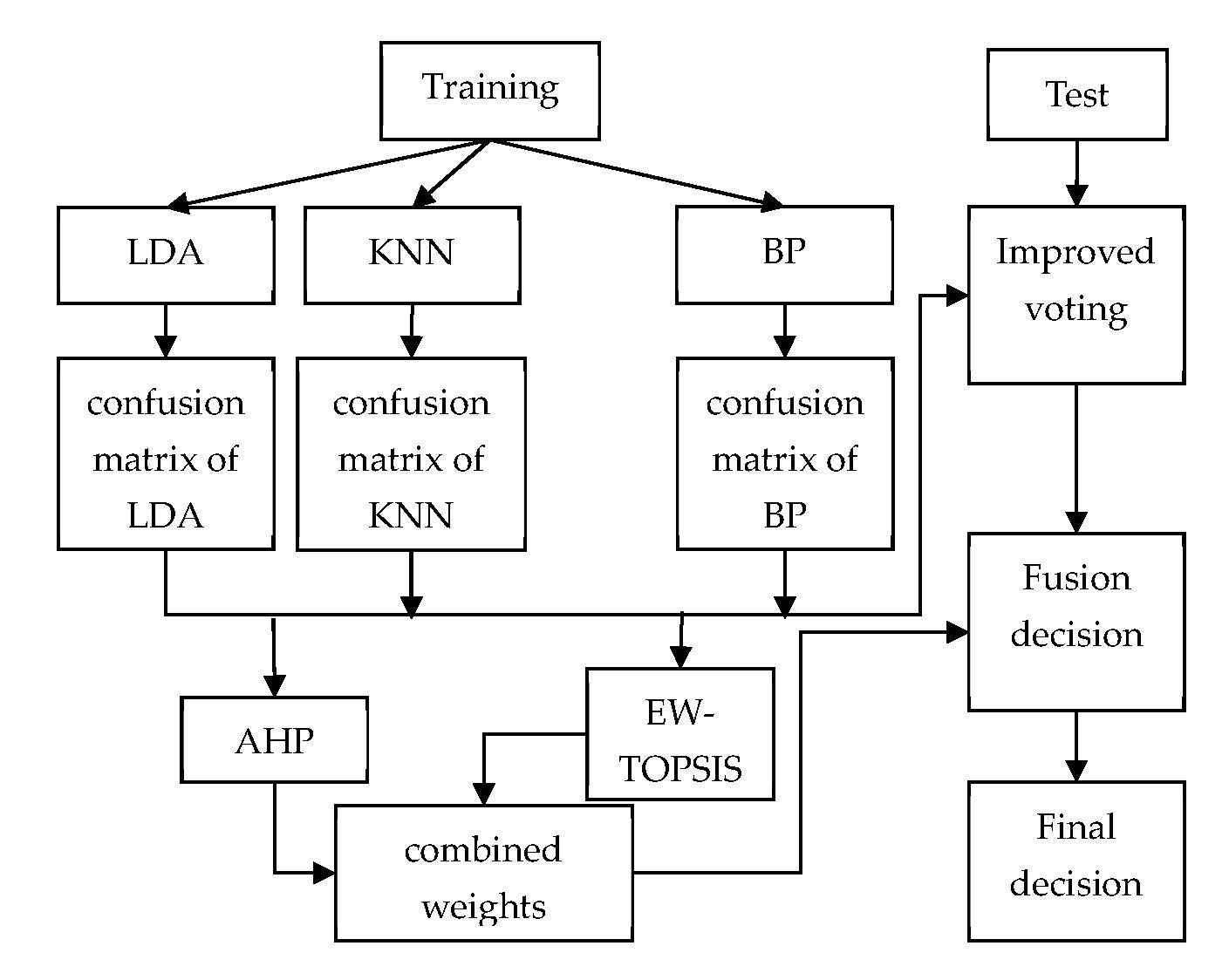
The ensemble method integrates various fault classification methods to improve the fault classification capability. A basic ensemble method includes the selection of base classifiers and the determination of fusion strategies. In this study, six basic classifiers were selected: linear discriminant analysis (LDA), K-nearest neighbor (KNN), Bayesian classifier (BN), random forest (RF), support vector machine (SVM) and the BP neural network (BP). Decision fusion is achieved by the CW and improved voting methods.

The specific framework of our proposed fusion system is shown in Figure 1.

3.1. Selection of Base Classifiers

Considering the requirement of diversity for the ensemble classification system, we selected six representative classifiers from the supervised category. Among them, LDA is a linear classifier, which is suitable for the classification of linear separable problems. KNN is a simple classifier, which determines the classification result by comparing the distance between the sample to be classified and all training samples. BN is one of the commonly used classifiers. It has an advantage in terms of classification speed and is suitable for applications with small-scale samples and missing values. RF is an integrated classifier based on the decision tree and has the advantage of a low computation cost. It can deal with high-dimensional samples and sample imbalance. The typical advantage of SVM is that it can use small samples and is also good for nonlinear problems. The BP neural network is a multi-layer feed-forward neural network with error backpropagation, which is advantageous for dealing with nonlinear problems.

3.2. Classifier Performance Evaluation

To measure the classification performance, four evaluation indicators were used [14]:

$$Accuracy\left(ACC\right)=\frac{numberoffaultsamplescorrectlyclassified}{samplenumberofallfaultsamples},$$

(21)

$$MissingRate\left(MR\right)=\frac{numberoffaultsamplesclassifiedasotherfaultsamples}{numberofallfaultsamples},$$

(22)

$$Precision\left(P\right)=\frac{1}{t}{\displaystyle \sum _{j=1}^t\frac{numberofsamplesclassifiedasfaultjandactuallyfaultj}{thenumberofsamplesclassifiedasfaultj}},$$

(23)

where t is the number of fault classes.

$$F-value\left(F\right)=\frac{2\times P\times R}{P+R},$$

(24)

where P is the precision and R is the recall rate.

The information used to calculate these performance evaluation indicators is given by the confusion matrix. The confusion matrix is also a way to measure the classifier’s performance, and its form is as follows [14]:

$$C{M}^k=\left[\begin{array}{ccc}{N}_{11}^k& \cdots & N_{1t}^k\\ ⋮& \ddots & ⋮\\ N_{t1}^k& \cdots & N_{tt}^k\end{array}\right],k=1,2,\cdots ,c,$$

(25)

where $N_{ij}^k$ represents the percentage of cases where fault i classified as fault j by classifier k. c is the number of base classifiers, and t is the number of fault classes.

3.3. Formatting of Mathematical Components

Voting is a simple and practical decision-making fusion strategy, but its fusion results are often unreasonable because it ignores the performance differences of various methods. In the process of fusion, the method with excellent performance should have greater/more influence on the voting results. This paper proposes a validity concept based on the confusion matrix to improve the voting method.

The concept of the validity value is defined as follows:

$$v_j^k=N_{jj}^k-\frac{{\displaystyle \sum _{i=1,i\ne j}^t{N}_{ij}^k}}{{\displaystyle \sum _{i=1}^t{N}_{ij}^k}},j=1,\cdots ,t,$$

(26)

where $v_j^k$ represents the validity of classifier k for fault j. The larger the value of $v_j^k$, the higher the credibility of the result when a test sample is classified as fault j by classifier k. Additionally, the following conditions should be met:

$$v_j^k=\{\begin{array}{c}0,v_j^k<0\\ v_j^k,v_j^k\ge 0\end{array}.$$

(27)

In the improved voting method, the voting result is determined by the validity value of the base classifier for different faults. Different from the conventional voting method, the fusion results given by the improved voting method are no longer crisp (i.e., either 0 or 1), but they take values in the interval of 0–1. This not only avoids the shortcomings of the original voting method, which does not consider the difference in performance of each classifier on different faults, but also enhances the impact of the classifiers with good performance in terms of voting results.

A validity matrix can be obtained by using the improved voting method:

$$V=\left[\begin{array}{ccc}{v}_1^1& v_2^1& \begin{array}{cc}\cdots & v_t^1\end{array}\\ \begin{array}{c}{v}_1^2\\ ⋮\end{array}& \begin{array}{c}{v}_2^2\\ ⋮\end{array}& \begin{array}{c}\begin{array}{cc}\cdots & v_t^2\end{array}\\ \begin{array}{cc}\cdots & ⋮\end{array}\end{array}\\ v_1^c& v_2^c& \begin{array}{cc}\cdots & v_t^c\end{array}\end{array}\right],j=1,\cdots ,t.$$

(28)

Combined with the combined weights, the decision of the fusion system is:

$$D=C{W}^{\mathrm{T}}\ast V=\left(d_1,d_2,\cdots ,d_t\right).$$

(29)

Finally, the maximum value is used as the fusion decision:

$$FD=\underset{j}{\arg \max }\left\{d_j\right\},j=1,2,\cdots ,t.$$

(30)

In summary, the proposed decision fusion system uses multiple performance evaluation indicators to measure the performance of the base classifier and determine the combined weights based on AHP and EW-TOPSIS for the base classifiers under these indicators. In addition, an improved voting method based on validity was developed to improve the effectiveness of decision fusion. In the next section, the proposed method is verified by the TE process.

4. Results

4.1. TE Process

The TE process is a test platform for complex chemical processes. It was proposed by Downs et al. [31] and has been widely used to evaluate the performance of process monitoring algorithms. The TE process mainly consists of five units: a reactor, a condenser, a compressor, a stripper, and a separator. It contains 53 variables, including 41 measurement variables and 12 manipulated variables. All 21 faults can be simulated on this test platform. Among them, faults 1–7 are step faults, faults 8–12 are random variation faults, and faults 16–20 are unknown faults. For more details, please refer to [31,32].

In this study, all 21 faults were used. The training set for each fault contained 380 samples, with each sample being 52-dimensional (the 12th manipulated variable of Agitator Speed was omitted). The validation data for each fault comprised 100 samples. The test sets for each fault contained 800 samples. The datasets can be downloaded from http://web.mit.edu/braatzgroup/links.html.

4.2. Experiment

The parameter settings of the base classifiers were as follows: the number of neighbors was 7 for the KNN classifier; the number of base decision trees was set to 100 for the RF classifier; and the grid parameters optimization method was used to determine the optimal parameters c and g of the SVM; the number of hidden layers of the BP neural network was set to 21, and the number of training iterations was 100.

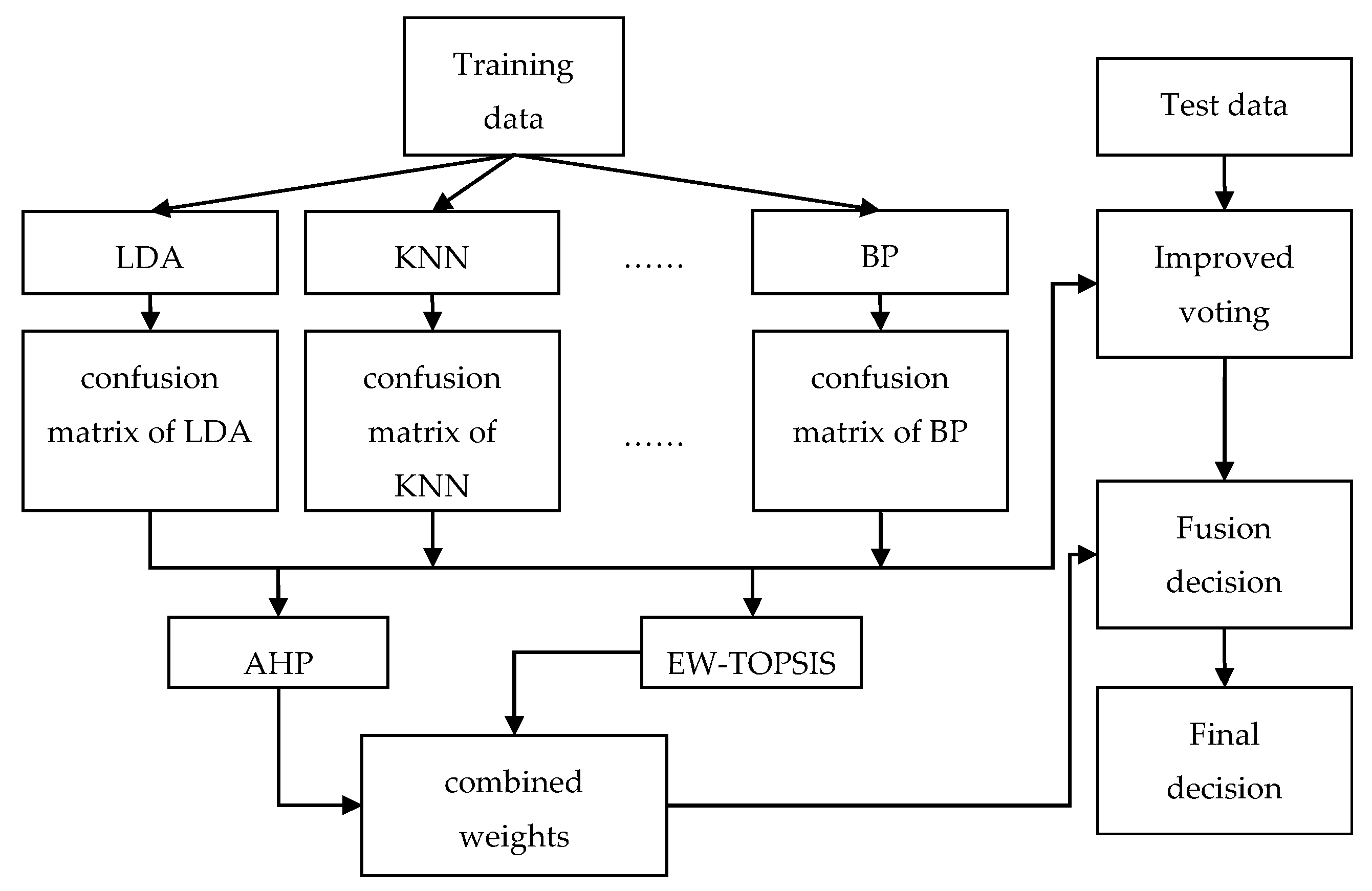
In this case, the confusion matrix of the six base classifiers was first determined. Then, the structure of the AHP was constructed based on four performance evaluation indicators and six base classifiers, as shown in Figure 2.

Next, we determined the importance of the four performance evaluation indicators and constructed a judgment matrix. The indicator F was considered to be the most important performance evaluation indicator, because it is the combination of the recall rate and precision. The indicator ACC can effectively display the classification accuracy of the classifier, so it was regarded as the second most important performance evaluation indicator. MR was also considered to be the second most important performance evaluation indicator. P was the third most important performance evaluation indicator. Combined with Table 1, the judgment matrix shown in

Table 3. Judgment matrix of the performance evaluation indicators.

Indicators	F	ACC	MR	P	Weights
F	1	2	2	3	0.4236
ACC	1/2	1	1	2	0.2270
MR	1/2	1	1	2	0.2270
P	1/3	1/2	1/2	1	0.1223

was obtained.

Where ${\lambda }_{\max }=4.0104$, $CI=0.0035$, $RI=0.90$, and $CR=0.0039$. The consistency check was satisfied.

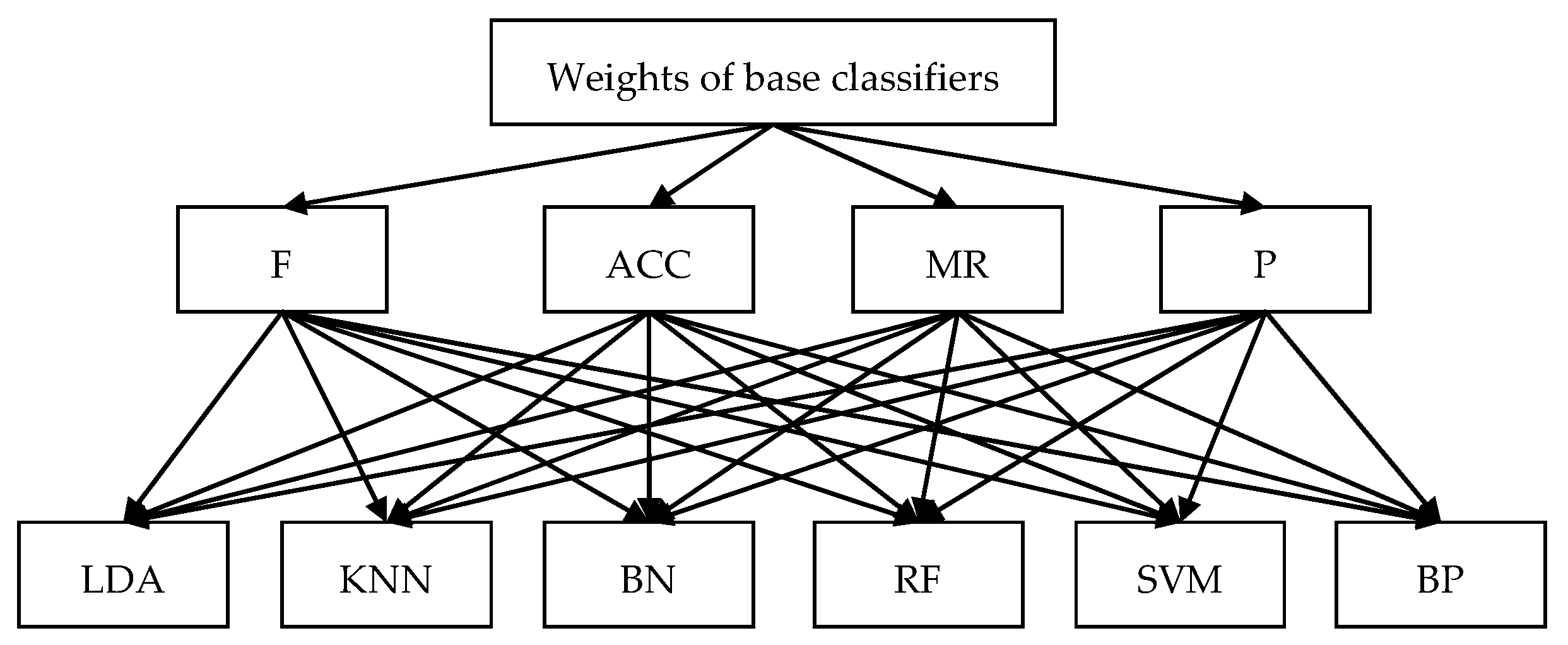
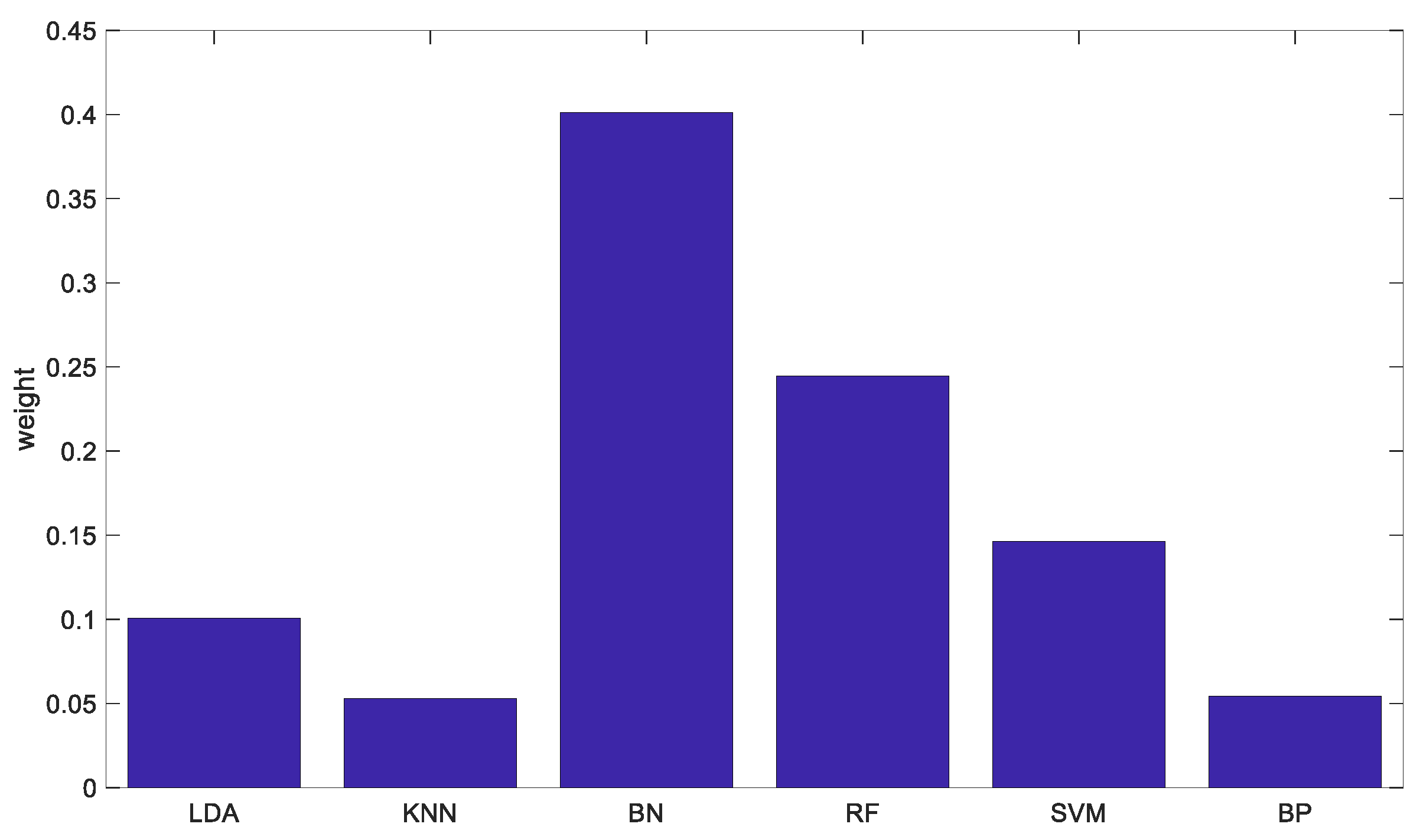
In the same way, the judgment matrix of the base classifier for each performance evaluation indicator was constructed in turn, and the judgment matrix was obtained according to the confusion matrix. Figure 3 shows the weight of each base classifier relative to each performance evaluation indicator. Finally, the weight of the basic classifier based on the AHP is shown in Figure 4.

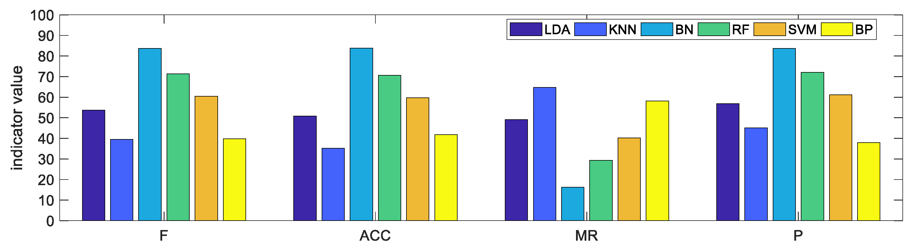
Performance evaluation indicators of each base classifier are calculated by the confusion matrix as shown in Figure 5.

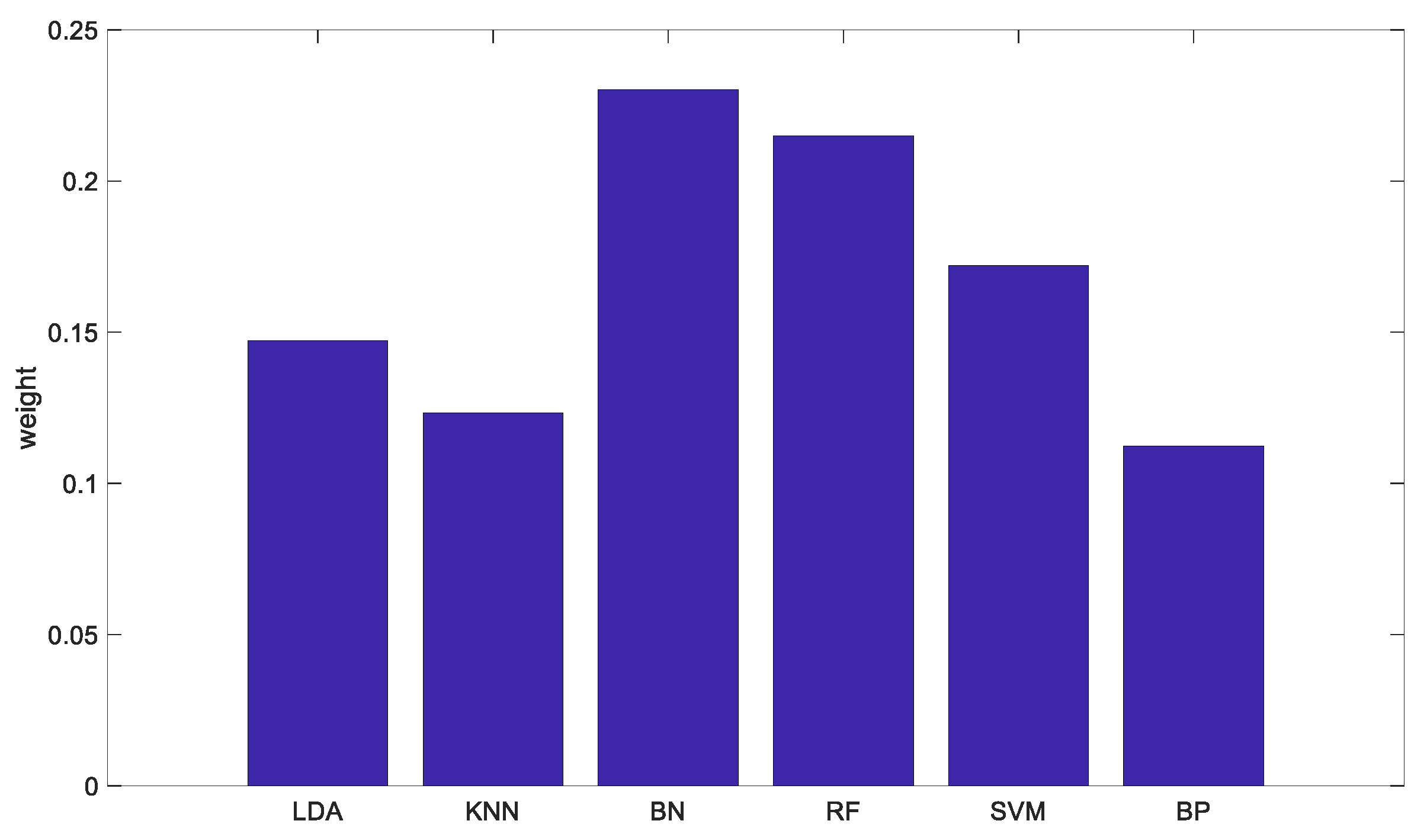
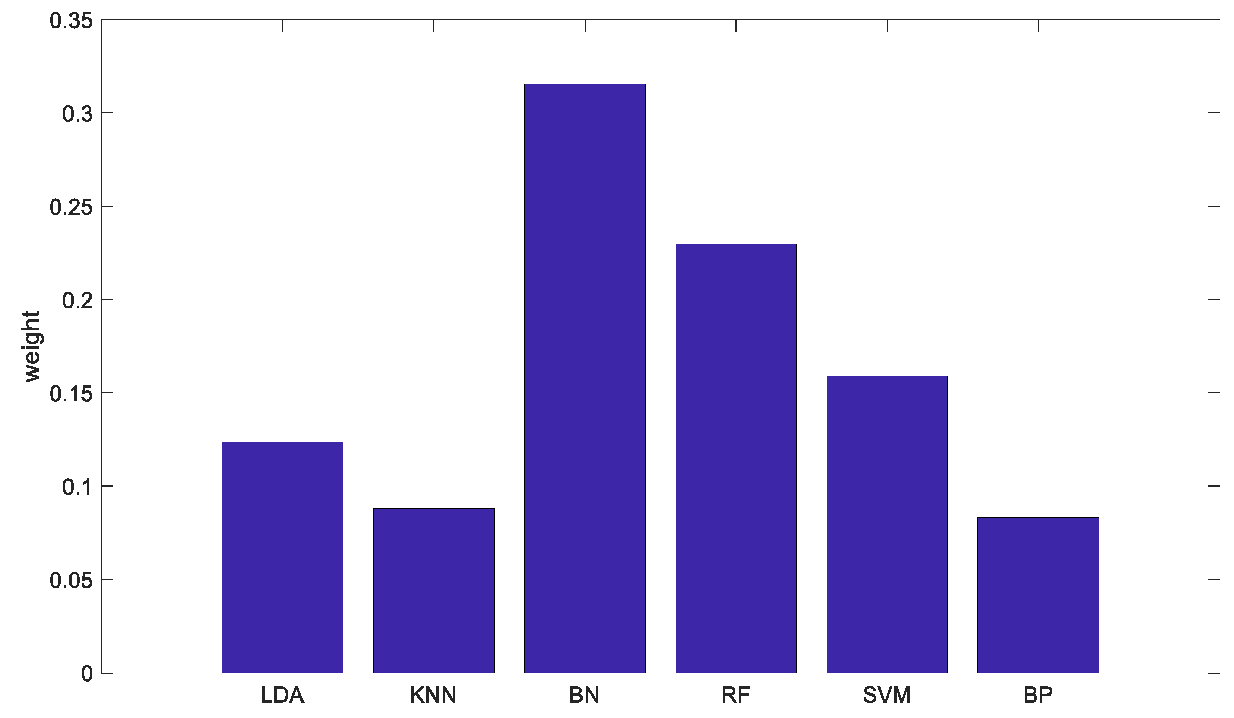
The weights of the base classifiers based on EW-TOPSIS are shown in Figure 6, and the CWs are shown in Figure 7.

For comparison, the classification accuracies of the six base classifiers and the proposed method are listed in

Table 4. Fault classification accuracy of various classifiers (%).

Fault No.	LDA	KNN	BN	RF	SVM	BP	VOTE	IVM	CWM	ETIVM	AIVM	CWIVM
1	98	98.13	98.63	98.5	98.63	98.63	98.88	99.13	98.88	99.13	98.88	98.88
2	96.25	97.5	98.25	98	97.88	98.75	98.38	99	98.25	98.38	98.25	98.25
3	11.25	21.25	17.25	17.38	19.13	0	24.63	14.25	17.5	12.63	11.63	11.38
4	81.5	20.75	73.63	95.13	89.13	11.13	97.63	99.5	94.38	98.63	98.38	98.38
5	98.5	20.5	98.13	51.63	98.13	95.38	99.38	99.13	99.13	99.13	98.13	98.88
6	99.75	99.75	56.38	99.38	63.13	33.88	100	100	100	100	63.13	100
7	100	80.38	100	99.75	100	100	100	100	100	100	100	100
8	37.13	28.75	96.5	53.25	34	54.63	71.88	78	83	90.38	96.13	95.25
9	14.25	13	21.63	17.25	15.75	0	19.13	7.88	20.38	7.75	13.25	10.5
10	40.13	8.13	83.75	43.38	21.38	0	53.25	78.63	75.25	82	83.75	83.75
11	8.63	8.63	70.75	62	15.63	0	37.5	45.5	62.5	59.75	62.25	61.63
12	31.25	29.75	97.25	76.63	60.5	2.25	73.75	83.13	89	86.63	94.5	91.63
13	20.75	16.5	57.75	16.5	12.25	22.13	19.13	28.38	37.63	36.75	51.38	49.63
14	7.75	44.25	97.25	94	72.5	0	85.13	93.13	94.13	93.25	97	94.25
15	15	14.25	26.25	26	18.88	0	20.63	26.75	26.63	28.13	31	30.63
16	37.75	7.5	79.25	48.25	20.75	29	51.5	73.38	70.25	76.63	79.13	78.75
17	51.75	39.13	86.5	90.38	73.63	84.38	87.38	92.88	90.13	92.63	89.5	91.75
18	16.5	81.25	18.63	86.13	62	70	86.13	88.75	86.5	88.88	51.5	88.5
19	14.5	29.88	94.38	78.13	49.38	0	68	93.5	89.5	95.38	95.25	95.75
20	52	12.63	87.5	61.38	47.38	79.13	72.5	89.13	84.13	88.25	87.5	87.63
21	5.75	6.25	99.25	24	2.75	38	30	93.5	80.38	98.88	99.75	99.75
Average	44.68	37.05	74.23	63.67	51.08	38.92	66.42	75.4	76.07	77.77	76.2	79.29

. Among them, VOTE represents the majority voting method, and IVM represents the improved voting method, CWM represents the classification accuracy when only the combination weights are used, ETIVM represents the combination of the objective weights and the improved voting method, AIVM represents the combination of the subjective weights and the improved voting method, and CWIVM represents the combination of combination weights and the improved voting method.

4.3. Discussion

The following conclusions can be drawn from the analysis of Table 4: Compared with the basic classifier, the average classification accuracies of IVM and CWM improved by at least 1.17% and 1.84%, respectively. Compared with the majority voting method, the average classification accuracies of IVM and CWM increased by 8.98% and 9.65%, respectively. This shows the effectiveness of IVM and CWM. Further, by analyzing the results of ETIVM, AIVM, and CWIVM, it can be seen that although the improved voting method can be further improved by combining the improved voting method with the weight of the base classifier determined by a single objective or subjective method, it is far less effective than the combination of the combined weight and the improved voting method. The average classification accuracy of CWIVM reached 79.29%—at least 5.06% and 12.87% higher than that of the base classifier and majority voting method, respectively.

However, the classification accuracy of the proposed method on faults 3, 9, and 15 was lower than 40%. This is unacceptable for industrial process monitoring, which need further investigation.

5. Conclusions

In this paper, a new ensemble classification system with combined weights and improved voting rules was presented. The combined weights were obtained by integrating the experts’ subjective weights and data-induced objective weights. The AHP and EW-TOPSIS were used to generate subjective weights and objective weights, respectively, for the base classifiers in the proposed fusion system. The concept of validity was defined in this paper in order to change the deficiencies of the conventional voting method, and a new voting method based on the validity was proposed to improve the fusion results. The experiments on the TE process demonstrate the effectiveness of the proposed method.

References

- Gao, Z.W.; Cecati, C.; Ding, S.X. A survey of fault diagnosis and fault-tolerant techniques part II: Fault diagnosis with knowledge-based and hybrid/active approaches. IEEE Trans. Ind. Electron. 2015, 62, 3768–3774. [Google Scholar] [CrossRef]
- Tidriri, K.; Chatti, N.; Verron, S.; Tiplica, T. Bridging data-driven and model-based approaches for process fault diagnosis and health monitoring: A review of researches and future challenges. Annu. Rev. Control 2016, 42, 63–81. [Google Scholar] [CrossRef]
- Zeng, L.; Long, W.; Li, Y. A novel method for gas turbine condition monitoring based on KPCA and analysis of statistics T2 and SPE. Processes 2019, 7, 124. [Google Scholar] [CrossRef]
- Wu, X.; Gao, Y.; Jiao, D. Multi-label classification based on random forest algorithm for non-intrusive load monitoring system. Processes 2019, 7, 337. [Google Scholar] [CrossRef]
- Dasarathy, B.V.; Sheela, B.V. A composite classifier system design: Concepts and methodology. Proc. IEEE 1979, 67, 708–713. [Google Scholar] [CrossRef]
- Polikar, R. Ensemble based systems in decision making. IEEE Circuits Syst. Mag. 2006, 6, 21–45. [Google Scholar] [CrossRef]
- Qu, J.; Zhang, Z.; Gong, T. A novel intelligent method for mechanical fault diagnosis based on dual-tree complex wavelet packet transform and multiple classifier fusion. Neurocomputing 2016, 171, 837–853. [Google Scholar] [CrossRef]
- Moradi, M.; Chaibakhsh, A.; Ramezani, A. An intelligent hybrid technique for fault detection and condition monitoring of a thermal power plant. Appl. Math. Model. 2018, 60, 34–47. [Google Scholar] [CrossRef]
- Pashazadeh, V.; Salmasi, F.R.; Araabi, B.N. Data driven sensor and actuator fault detection and isolation in wind turbine using classifier fusion. Renew. Energy 2018, 116, 99–106. [Google Scholar] [CrossRef]
- Kannatey-Asibu, E.; Yum, J.; Kim, T.H. Monitoring tool wear using classifier fusion. Mech. Syst. Signal Proc. 2017, 85, 651–661. [Google Scholar] [CrossRef] [Green Version]
- Ng, Y.S.; Srinivasan, R. Multi-agent based collaborative fault detection and identification in chemical processes. Eng. Appl. Artif. Intell. 2010, 23, 934–949. [Google Scholar] [CrossRef]
- Chen, Y.; Cremers, A.B.; Cao, Z. Interactive color image segmentation via iterative evidential labeling. Inf. Fusion 2014, 20, 292–304. [Google Scholar] [CrossRef]
- Lin, Y.; Wang, C.; Ma, C.; Dou, Z.; Ma, X. A new combination method for multisensor conflict information. J. Supercomput. 2016, 72, 2874–2890. [Google Scholar] [CrossRef]
- Liu, Y.; Ni, W.; Ge, Z. Fuzzy decision fusion system for fault classification with analytic hierarchy process approach. Chemom. Intell. Lab. Syst. 2017, 166, 61–68. [Google Scholar] [CrossRef]
- Ge, Z.; Liu, Y. Analytic hierarchy process based fuzzy decision fusion system for model prioritization and process monitoring application. IEEE Trans. Ind. Inform. 2019, 15, 357–365. [Google Scholar] [CrossRef]
- Saaty, T.L. How to make a decision: The analytic hierarchy process. Eur. J. Oper. Res. 1990, 48, 9–26. [Google Scholar] [CrossRef]
- Shi, L.; Shuai, J.; Xu, K. Fuzzy fault tree assessment based on improved AHP for fire and explosion accidents for steel oil storage tanks. J. Hazard. Mater. 2014, 278, 529–538. [Google Scholar] [CrossRef]
- Tang, Y.; Sun, H.; Yao, Q.; Wang, Y. The selection of key technologies by the silicon photovoltaic industry based on the Delphi method and AHP (analytic hierarchy process): Case study of China. Energy 2014, 75, 474–482. [Google Scholar] [CrossRef]
- Samuel, O.W.; Asogbon, G.M.; Sangaiah, A.K.; Fang, P.; Li, G. An integrated decision support system based on ANN and Fuzzy_AHP for heart failure risk prediction. Expert Syst. Appl. 2017, 68, 163–172. [Google Scholar] [CrossRef]
- Sara, J.; Stikkelman, R.M.; Herder, P.M. Assessing relative importance and mutual influence of barriers for CCS deployment of the ROAD project using AHP and DEMATEL methods. Int. J. Greenh. Gas Control 2015, 41, 336–357. [Google Scholar] [CrossRef]
- Kumar, R.; Anbalagan, R. Landslide susceptibility mapping using analytical hierarchy process (AHP) in Tehri reservoir rim region, Uttarakhand. J. Geol. Soc. India 2016, 87, 271–286. [Google Scholar] [CrossRef]
- Wang, T.; Chen, J.S.; Wang, T.; Wang, S. Entropy weight-set pair analysis based on tracer techniques for dam leakage investigation. Nat. Hazards 2015, 76, 747–767. [Google Scholar] [CrossRef]
- Schneider, E.R.F.A.; Krohling, R.A. A hybrid approach using TOPSIS, Differential Evolution, and Tabu Search to find multiple solutions of constrained non-linear integer optimization problems. Knowl. Based Syst. 2014, 62, 47–56. [Google Scholar] [CrossRef]
- He, Y.H.; Wang, L.B.; He, Z.Z.; Xie, M. A fuzzy TOPSIS and rough set based approach for mechanism analysis of product infant failure. Eng. Appl. Artif. Intell. 2016, 47, 25–37. [Google Scholar] [CrossRef]
- Patil, S.K.; Kant, R. A fuzzy AHP-TOPSIS framework for ranking the solutions of Knowledge Management adoption in Supply Chain to overcome its barriers. Expert Syst. Appl. 2014, 41, 679–693. [Google Scholar] [CrossRef]
- Wu, J.; Li, P.; Qian, H.; Chen, J. On the sensitivity of entropy weight to sample statistics in assessing water quality: Statistical analysis based on large stochastic samples. Environ. Earth Sci. 2015, 74, 2185–2195. [Google Scholar] [CrossRef]
- Ji, Y.; Huang, G.; Sun, W. Risk assessment of hydropower stations through an integrated fuzzy entropy-weight multiple criteria decision making method: A case study of the Xiangxi River. Expert Syst. Appl. 2015, 42, 5380–5389. [Google Scholar] [CrossRef]
- Yan, J.; Feng, C.; Li, L. Sustainability assessment of machining process based on extension theory and entropy weight approach. Int. J. Adv. Manuf. Technol. 2014, 71, 1419–1431. [Google Scholar] [CrossRef]
- Kou, G.; Peng, Y.; Wang, G. Evaluation of clustering algorithms for financial risk analysis using MCDM methods. Inf. Sci. 2014, 275, 1–12. [Google Scholar] [CrossRef]
- Nyimbili, P.; Erden, T.; Karaman, H. Integration of GIS, AHP and TOPSIS for earthquake hazard analysis. Nat. Hazards 2018, 92, 1523–1546. [Google Scholar] [CrossRef]
- Downs, J.J.; Vogel, E.F. A plant-wide industrial process control problem. Comput. Chem. Eng. 1993, 17, 245–255. [Google Scholar] [CrossRef]
- Russell, E.L.; Chiang, L.H.; Braatz, R.D. Data-Driven Techniques for Fault Detection and Diagnosis in Chemical Processes; Springer: London, UK, 2000. [Google Scholar]
Figure 1.
Decision fusion system based on combination weights and the improved voting method. AHP: analytic Hierarchy Process; BP: BP neural network; EW-TOPSIS: entropy weight-technique for order performance by similarity to ideal solution; KNN: K-nearest neighbor; LDA: linear discriminant analysis.
Figure 2.
Hierarchy of the AHP. BN: Bayesian classifier; RF: random forest; F: F-value; ACC: Accuracy; MR: Missing Rate; P: Precision.
Figure 3.
Weight of each base classifier relative to each performance evaluation indicator.
Figure 4.
AHP-based classifier weights.
Figure 5.
Value of each base classifier relative to each performance evaluation indicator.
Figure 6.
EW-TOPSIS-based classifier weights.
Figure 7.
Combined weight (CW)-based classifier weights.