Data Augmentation Applied to Machine Learning-Based Monitoring of a Pulp and Paper Process

Abstract

Industrial archived process data represent a convenient source of information for data-driven models, such as artificial neural network (ANN), that can be used for safety and efficiency improvement like early or even predictive fault detection and diagnosis (FDD). Nonetheless, most of the data used for model generation are representative of the process nominal states and therefore are not enough for classification problems intended to determine abnormal process conditions. This work proposes the use of techniques to augment the original real data standards, dismissing the need for experiments that could jeopardize process safety. It uses the Monte Carlo technique to artificially increase the number of model inputs coupled to the nearest neighbor search (NNS) by geometric distances to consistently classify the generated patterns in normal or faulty statuses. Finally, a radial basis function neural network is trained with the augmented data. The methodology was validated by a study case in which 3381 pulp and paper industrial data points were expanded to monitor the formation of particles in a recovery boiler. Only 5.8% of the original process data were examples of faulty conditions, but the new expanded and balanced data collection leveraged the classification performance of the neural network, allowing its future use for monitoring purpose.

1. Introduction

Even though modern process control systems in chemical industries are highly automatic, the automation of abnormal situation management is yet to be accomplished. According to Venkatasubramanian [1], the UK loses 27 billion dollars per year due to abnormal situations, and Vásquez and co-workers [2] report that the economic losses of the petrochemical industry in the USA are up to 20 billion dollars per year.

Continuous process monitoring in association with fault detection and diagnosis (FDD) tools might contribute greatly to achieve operational excellence by optimizing maintenance interventions and avoiding unplanned shutdowns and even preventing accidents.

Several approaches have been developed over the years to cope with the FDD issues in industrial processes. Venkatasubramanian, Rengaswamy, and Kavuri [3,4,5] summarize and review the main characteristics of the techniques described in the literature. Nonetheless, the size and complexity of chemical process industries and the increasing amount of data available in this digital era endorse the use of data-based FDD techniques, such as neural network algorithms and multivariate statistical methods [6]. Ragabab and co-workers, Casanova-Peláez and co-workers, and Leiviskä [7,8,9] are some examples of data-driven FDD applications in chemical processes applications.

There are still many challenges until FDD becomes widespread in industrial applications. Most of the historical data used for model generation are representative of process nominal states. Therefore, the data collection contains limited information, corresponding to a specific time window and is possibly limited to a set of operational states’ space regions. In industrial processes, the low data of faulty conditions or non-uniform data distributions are common because processes are not allowed to operate in faulty scenarios for safety reasons. When data distributions are unbalanced, it is difficult to use the data information samples to construct an accurate classifier for conventional machine learning algorithms [10]. The categories with low data, such as unusual faults, are easily neglected and submerged by the situations with a large amount of samples, and the classification algorithm becomes biased towards majority classes [11].

Venkatasubramanian [12] highlights that a drawback of machine learning data-centered techniques is that a tremendous amount of data is required. Even though we collect much more data now than we did in the past, the chemical processes “big data” domain is not like finance, vision, game playing, and speech domains. Chemical processes data usually deal with incomplete and noisy measurements. Clinical decision making [13] and civil and structural engineering [14] are also subjected to such data issues.

Many research efforts to address the unbalanced dataset issue focus on two different approaches: Improved algorithms and data preprocessing techniques [10]. The improved algorithms do not create a balanced data distribution. Instead, they highlight the unbalanced learning problem by using cost-sensitive learning, ensemble learning, or probability density changes techniques [15,16,17,18]. Nonetheless, too many computational resources and time are consumed by algorithm-level methods [15].

The data-level approach consists of re-sampling methods, which mainly include increasing the number of minority examples by replicating observations in the original dataset—over-sampling—or decreasing the number of majority examples by removing some of them—under-sampling [19,20,21,22]. Duplications and uncertainties are introduced by re-sampling methods that might lead to overfitting or loss of information [15].

Data augmentation (DA) seems to be an alternative to overcome the unbalanced dataset issue by artificially inflating the training set with label-preserving transformations [23]. DA methods are traditionally used in the image domain to synthesize data samples by geometric transformations, such as rotation, brighten, clips, flips, and channel alterations [24]. This DA approach is called data warping [15], a computationally inexpensive method [25], which generates additional samples through transformations applied in the data space. However, the generated data is just a surfaced transformation of the original data, and the traditional transformation technique can only be used in the image sets [26]. Another DA approach for creating additional training samples is synthetic over-sampling, which creates additional samples in the feature space [15]. This scheme has the ability to generate a greater variety of data [23]. Previous researches demonstrated that data augmentation works as a regularizer that avoids overfitting and improves model performance. Zaifeng et al. [27] focused on image analysis with augmented data. Huang and co-workers [28] used a generative adversarial network with a gradient penalty (GAN) data augmentation technique for marine organisms’ detection and recognition, and Gao et al. [11] used GAN-based data augmentation to deal with unbalanced data sets for FDD in chemical industrial benchmarks. Zhou et al. [29] also used GAN to generate more discriminant fault samples. The authors of [30,31,32] discussed synthetic minority over-sampling technique (SMOTE) applications.

The pulp and paper industry is one of the largest industries in the world, considering that paper has many powerful benefits to human society through education, communication, security, and hygiene. The world’s paper production was around 406 million tons in 2015 and it is expected to reach 482 million tons by 2030. Brazil is the fourth largest producer of pulp in the world and the ninth largest producer of paper [33]. Nevertheless, in recent years, pulp and paper mills have faced challenges concerning energy efficiency mechanisms and management of the resulting pollutants, considering the environmental feedbacks and the competitive markets [34].

Globally, more than half of the produced paper is used for packaging (cartonboard and containerboard). There have been substantial reductions in the consumption of printing and writing paper since 2010, which represents a 25% reduction in the volume of paper use. In the last years, sanitary paper consumption represents the highest growth rate, although it accounts for less than 10% of the global volume at the present [34].

The kraft process is the dominant chemical route in the paper industry and uses sodium hydroxide (NaOH) and sodium sulphide (Na₂S) to pulp wood [35]. In this process, the wood is dissolved in pulping chemicals to form a liquid stream called weak black liquor (BL). The BL is washed out from the pulp and is sent to the kraft recovery boiler, where the inorganic pulping chemicals are recovered for reuse. Meanwhile, the dissolved organics are used as fuel to generate steam and power. In this process, every ton of produced pulp generates about 10 tons of weak black liquor or about 1.5 tons of black liquor dry solids that need to be processed through the chemical recovery process [36].

BL is the fifth most important fuel in the world. Every year, 1.3 billion tons of BL are processed in recovery boilers worldwide, recovering 15 million tons of cooking chemicals, reducing the amount of waste, and producing 700 million tons of steam at elevated pressure [35,37,38].

Despite its importance for increasing the process efficiency and reducing environmental impacts, the kraft recovery process is difficult to operate. Typical recovery boiler problems include the fouling of heat transfer tubes and plugging of flue gas passages by fireside deposits, which cause low steam production, blackouts, and air emissions, and lead to unscheduled operational shutdown [36]. Many of the recovery boiler’s issues might be caused by particle formation and deposition, a slow dynamic phenomenon that is difficult to monitor and predict.

Usually, slow dynamic phenomena are difficult to track and demand maintenance interventions like cleaning and regeneration procedures [39]. Therefore, the number of particles formed inside the boiler is a parameter that assists the evaluation of the operation, and the frequency of maintenance interventions can be reduced by using it as a process control variable.

The complex nature of the formation of particulate material inside the boiler makes it difficult to develop conventional mathematical models based on analytical and phenomenological methods. As a result, the use of artificial intelligence and machine learning techniques are an alternative to address this limitation. Artificial neural networks (ANNs) are processing techniques that use empirical information to generate complex system models through the identification and generalization of patterns found in a given data set. They are endowed with the capacity of learning from examples and are part of the artificial intelligence and machine learning methods.

This work proposes the use of the Monte Carlo simulation to artificially increase the amount of the original real data collection, leading to an expanded and widespread data set that represents nominal steady states and faulty conditions. The methodology used geometric distances and the nearest neighbors search to preserve the phenomenological characteristics of the original data set. The suggested technique was validated in a pulp and paper industrial study case wherein 3381 process data standards were expanded to monitor the formation of particles in a recovery boiler—a key equipment in kraft’s pulp and paper production plants. The new expanded and balanced data collection was used to develop an artificial neural network model to classify the operational status as normal or failure, allowing its future use for monitoring.

The paper is structured as follows: In Section 2, the industrial study case is presented, the real process data set characteristics are explained, and the normal and faulty scenarios are described. In Section 3, the data augmentation methodology and the model development steps are described. It includes the description of the statistical metrics used to assess the methodology performance: receiver operating characteristic (ROC) curve, confusion matrix, and true and false positive/negative ratios. In Section 4, the results are presented and compared to regular machine learning-based FDD model development and to previous research in the literature. The paper ends with the presentation of the main conclusions.

2. Case Study

This study presents real operational data of an important Brazilian pulp and paper mill, whose name was omitted for confidentiality. The data set corresponds to 12 months of operation of the recovery boiler of a kraft production process and includes 12 process variables and 3381 cases, acquired through the industrial SCADA system [40].

Table 1. Industrial process variables.

TAG	Description	Units
Vvlu	Black liquor feed flow rate	m³/h
x	Solids concentration in black liquor feed	%
Tlu	Black liquor feed temperature	°C
Var1	Primary air flow rate	ton/h
Var2	Secondary air flow rate	ton/h
Var3	Tertiary air flow rate	ton/h
Par1	Primary air feed pressure	mmH2O
Par2	Secondary air feed pressure	mmH2O
Tar1	Primary air feed temperature	°C
Tar2	Secondary air feed temperature	°C
Pl	Black liquor feed pressure	Kgf/cm²
Epart	Number of formed particles	Particles/min

shows the process variables and their physical description.

The Epart value is defined as the average number of particles formed inside the boiler that are dragged by the gas flow in the furnace at the entrance of the superheater region. Measurements are made by means of image processing captured by two cameras on both the right and left sides of the superheater section.

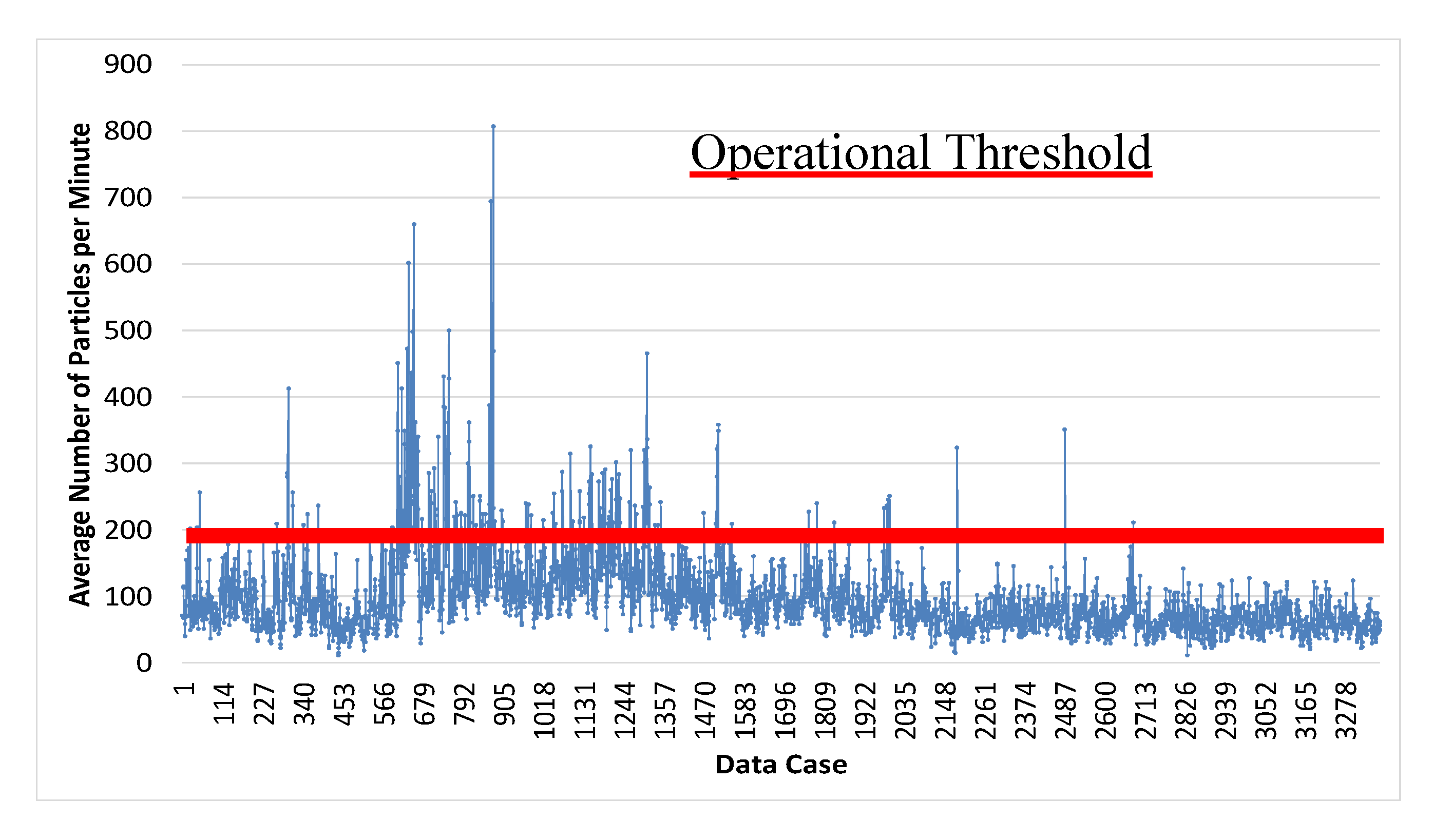
The operational data collected was preprocessed to deal with spurious data. Whenever the difference between the two camera sensors was greater than 100 particles per minute the operational case was withdrawn [40]. The Epart values ranged from 9.62 up to 806.12 particles per minute, where 200 particles per minute corresponds to normal operating conditions. This threshold is exceeded sometimes, characterizing the fault operating condition. There are 197 operational cases wherein the Epart values were greater than 200 particles per minute (5.8% of the total).

Figure 1 shows the real process operating conditions in which a faulty status is characterized by an average number of particles greater than 200/min. A non-uniform distribution is expected because the data points were gathered during routine operation in order to monitor the process and not to perform an experimental scan of all possible Epart values. The low number of points with high Epart values (above 200) shows that the boiler works most of the time within the desired operating conditions.

However, when the data is poorly distributed, the network training process can be impaired, a relevant issue for process control and FDD applications. For instance, if a certain class presents enough training standards, the network will classify with a high accuracy rate the data belonging to this specific class. However, if a class is not well trained, the network will be unable to perform generalization and will not classify future entries belonging to it. Thus, it is possible that the network presents a high overall performance, once it can classify most of the operational cases correctly. Yet, it performs poorly for one of the classes, which is not desired. In process control, a network that represents the normal operating situations well but cannot represent an abnormal situation might lead to unsafe scenarios.

3. Methodology

Monte Carlo simulation is a powerful statistical analysis tool that does not require physical experiments and conducts a large number of computerized experiments. It is named after the city of Monte Carlo in Monaco, which is famous for gambling, because it involves generating chance variables and exhibits random behaviors. It is particularly suitable for solving complex engineering problems because it can deal with many random variables, various distribution types, and highly nonlinear engineering models [41].

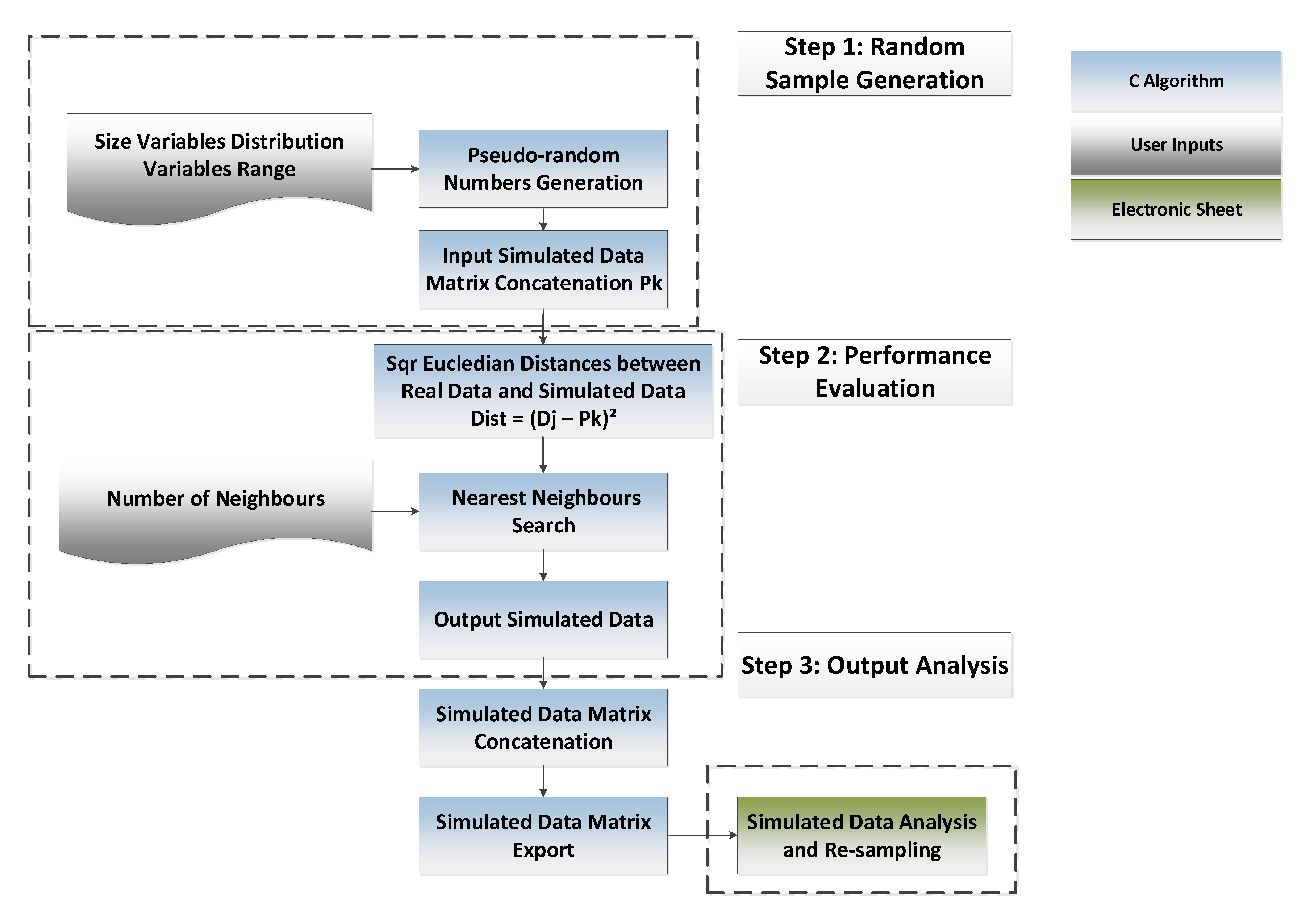
The Monte Carlo combined with a clustering technique implemented here for data augmentation can be depicted in three steps, as shown in Figure 2. In Monte Carlo-based step 1, n pseudo-random input variables with a normal distribution are generated using an algorithm in C programming language (see Equation (1)). Rand is a pseudo-random number that ranges between 0 and 1. The minimum and maximum values are limited to the real process data range and the number of generated cases is defined by the user. This step led to a large matrix with 11 columns—one for each input process variable—and n lines:

$$P=D_{Mín}+\left(D_{Máx}-D_{Mín}\right)*rand.$$

(1)

Then, the values of the output variable are calculated through the performance function at the n cases: A combination of geometric distance measurements with clustering analysis that establishes a decision rule to classify the n cases depending on the process features. This work used square Euclidian distances between the process plant data and the simulated data and the nearest neighbors search to define whether the operation was under normal or faulty conditions. The geometric distances were weighted by the inverse of the maximum values of the input (D_jMax) process variables to avoid the influence of their magnitude order, according to Equation (2):

$$Dis{t}_{kj}={\displaystyle \sum }\frac{{\left(D_{j,i}-P_k\right)}^2}{D_{jMax}};k=1:n\hspace{1em}i=1:l,$$

(2)

where:

• n—number of generated cases;
• l—length of real process data matrix;
• D_j—real process data matrix;
• P_k—simulated process data matrix; and
• D_jmax—real process data maximum values.

In step 2, the nearest neighbors clustered operational conditions alike to the simulated case being evaluated. The output variable (class) was hence determined by the arithmetic mean of the nearest neighbors classes, keeping the original real data representativity (true label) in the augmented categorical data collection.

By performing the output analysis of step 3, if the output data set retains the original unbalanced distribution, it is possible to resample it so that the new data collection exhibits a uniform distribution.

The statistical characteristics of the experiments (model outputs), such as data correlation, are observed and used to develop classification models intended for process fault detection and diagnosis (FDD) (Figure 3).

Radial basis function networks (RBFNs) were developed in the commercial software STATISTICA^® (version 12, Stata®, TX, USA, 2013), using uniformly distributed simulated data sets that differed in size. RBFN typically outperforms other traditional machine learning algorithms for classification problems when there is a representative training data set because they use an explicit similarity-metric classifier to make decisions, leading to a more robust decision boundary [42]. 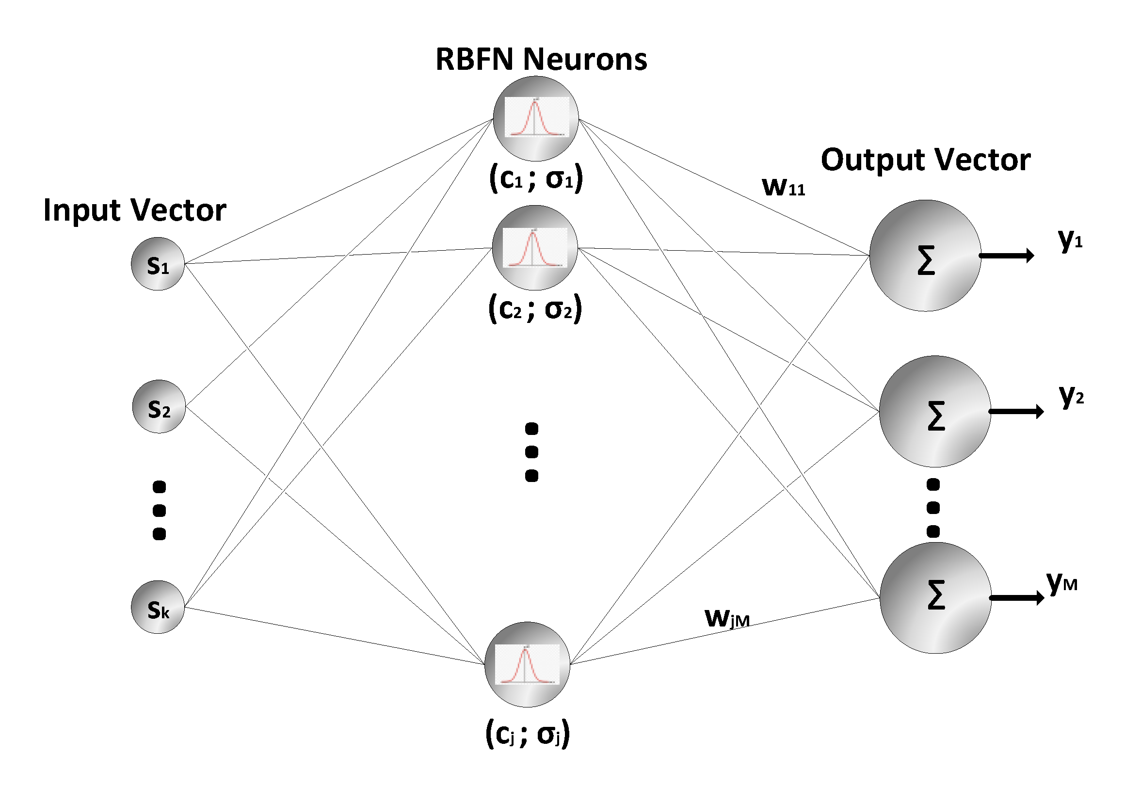Figure 4 presents the RBFN three-layer neural network scheme, in which the input vector is the first layer, the hidden layer containing the radial basis function neurons is the second layer, and the output layer consisting of linear neurons is the third layer.

The activation function of the hidden neurons is the Gaussian function, in which each neuron is represented by a bell curve centered at a given input value, called c. When a new input, s, is presented to the network, the neuron activation function classifies its similarity to all of the neurons of the network. The activation region is determined as a function of the Euclidean distance between the s input vectors and their center, c, weighted by the constant scale factor, σ (Equation (3)):

$$f\left(\underset{\_}{c_j},\underset{\_}{{\sigma }_j}\right)=e^{\left(-\frac{\parallel \underset{\_}{s_p}-{\underset{\_}{c_j}\parallel }^2}{{\underset{\_}{{\sigma }_i}}^2}\right)},$$

(3)

where:

• s_p—is the pth input vector presented to the network;
• c_j—is the center vector of the jth hidden neuron; and
• σ_j—constant scale factor value for the jth hidden neuron.

The activation, λ_pj, for the jth output neuron, relative to the pth input vector, is given by the sum of all hidden neuron outputs weighted by its respective weights. The softmax activation function, described in Equation (4) for the jth neuron, is then used to provide the normalized output of the RBFN, where it is admitted that the output layer has M neurons:

$$f\left({\mathsf{\lambda }}_{\mathrm{pj}}\right)=\frac{e^{{\mathsf{\lambda }}_{\mathrm{pj}}}}{{{\displaystyle \sum }}_{m=1}^M{e}^{{\mathsf{\lambda }}_{\mathrm{pm}}}}.$$

(4)

The initial learning phase of an RBFN is an unsupervised data-clustering phase, wherein the c centers are adjusted by the k-means algorithm. Then, the σ scale factors are adjusted by the P-nearest neighbor heuristic method. Finally, the w weights are calculated by the supervised backpropagation algorithm [42].

The simulated data matrix is the input-output pattern collection that will be used for the fault detection model’s development and its size will affect the quality of the monitoring predictions. A large number of features (or input variables) can lead to numeric difficulties in obtaining good class estimation. In this case, the classifier could be biased, fitted to the training set, due to the finiteness of the training set. Typically, the classifier is able to generalize when the number of cases, n, is sufficiently larger than the number of features, d [43].

The choice of an adequate dimensionality ratio (n/d) was based on power analysis and sample size estimation. If the pattern matrix size is too small, the empirical model will lack the precision to provide reliable answers to the investigative question. Nonetheless, if it is too large, time and resources will be wasted [43].

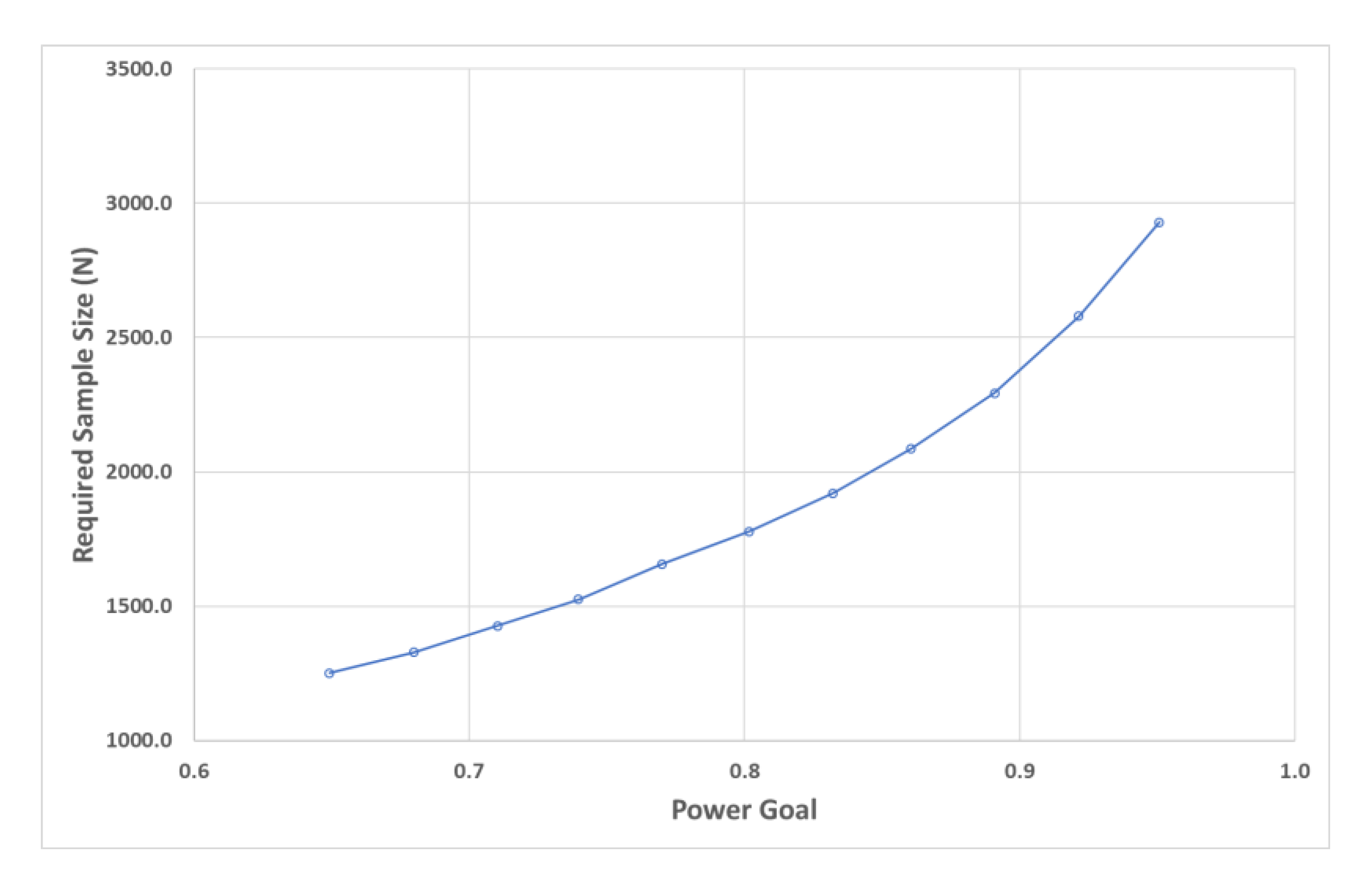
Briefly, power analysis is the hypothesis test that computes the probability of finding an existing effect [44]. The first option to increase the test performance within a significant tolerance is to increase the sample size. This work used a minimum acceptable power of 90% and a confidence level of 5%. The mean values of the population for the significance test were the integer values 1 and 2 markers attributed to each process class or status. The sample size estimation results are displayed graphically and allowed the determination of the pattern matrix size used for the RBFN FDD model development.

The RBFN classification tool is a non-parametric method and, therefore, makes no assumptions about the underlying data distribution.

Table 2. Neural network development parameters.

Parameter	Values
Number of Neural Networks developed	1000
Training Sample	80% of the data set
Test Sample	20% of the data set
Number of hidden neurons	10 to 100
Input Variables	Vvlu, x, Tlu, Var1, Var2, Var3, Par1, Par2, Tar1, Tar2, PI
Number of neural networks retained	10

summarizes the ANN model development parameters.

Each test generated 1000 new neural networks and the architectures presenting the best performance were selected and used for refining the search. This process was repeated until there was no significant performance improvement. Overall performance evaluation for both training and test phases were measured by the functions sum of squared error (SOS) and cross entropy (CE), described in Equations (5) and (6). The percentage of correct classifications for each class is presented as a confusion matrix:

$$E_{SOS}={{\displaystyle \sum }}_i^N{\left(y_i-t_i\right)}^2,$$

(5)

$$E_{CE}=-{{\displaystyle \sum }}_i^N{t}_i\times ln\left(\frac{y_i}{t_i}\right),$$

(6)

where:

• y_i—is the output value predicted by the ANN;
• t_i—is the target output value; and
• N—is the training data set size.

Global statistical sensitivity analysis is used to determine the importance of each input variable in the ANN model performance by the ratio of a new error (maintaining the evaluated variable constant at its average value) and the original error. High ratio values indicate that the input variable has a great influence on the neural network results.

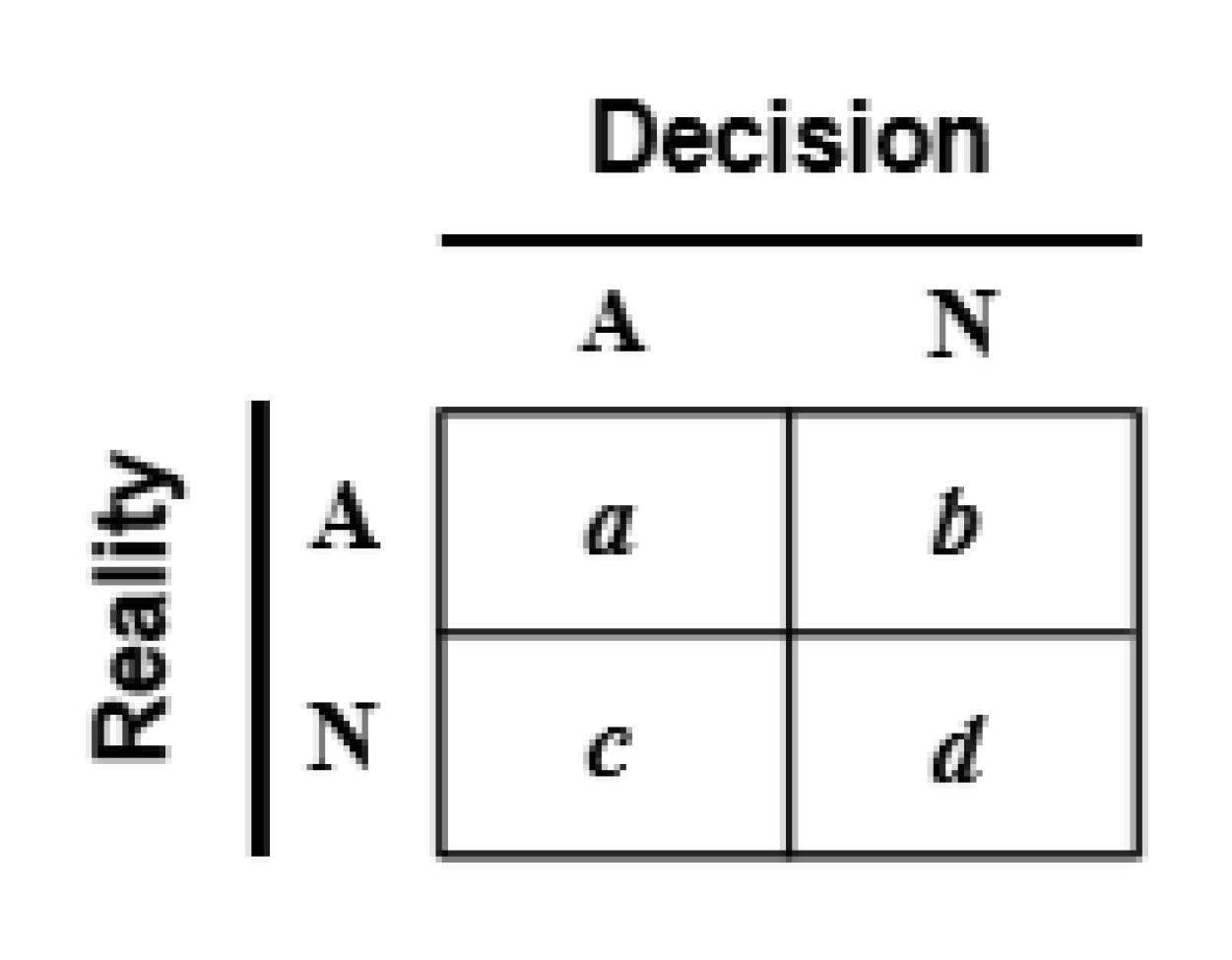
The best ANN model concerning training and recall performance was validated with real process data. The results were displayed by the confusion matrix and the ROC (receiver operating characteristic) curve. The ROC curve is an analysis tool for two-class problems that are intended to detect rarely occurring events, such as process faults [43]. Figure 5 shows the canonical classification matrix for this situation, with N being the normal event and A being the abnormal process condition. Based on a given decision rule, the true classes are exhibited along the rows and the predicted or decided classifications are displayed along the columns.

The ROC analysis method depicts the true positive ratio (TPR, in Equation (7))—or sensitivity-versus the false positive ratio (FPR, in Equation (8))—or the complement of the specificity—for every possible decision threshold [43]:

$$TPR= \frac{a}{a+b},$$

(7)

$$FPR=1- \frac{d}{c+d}.$$

(8)

It is expected that a classification method with high sensitivity, i.e., high true positive ratio and low false positive ratio, will rarely miss the abnormal event when it occurs. A classifier with a high specificity, i.e., high true negative ratio and low false negative ratio, will have a very low rate of false alarms. False alarms occur when normal events are classified as abnormal. A decision method is considered highly accurate if it simultaneously has a high sensitivity (rarely misses the abnormal event when it occurs) and a high specificity (has a low false alarm rate) [43]. Nonetheless, there is a compromise between sensitivity and specificity, graphically presented in the ROC curve. The classification method optimal performance for a large range of prevalence situations occurs when the ROC curve is close to perfect, i.e., with an underlying area of 1.

4. Results and Discussion

The Monte Carlo simulation generated 160,000 new patterns, creating specific faulty situations that are either impossible or too expensive to be forced to happen in the real world and too complex to be theoretically modeled by first principle equations. The data simulation step lasted about 8 h. Computational time was measured in an Intel^® Core™ i7-8550U processor (Intel, Santa Clara, CA, USA, 2017) running at 2 GHz in the Windows 10 operating system (Microsoft, Redmond, WA, USA,.2015).

In this new data collection, despite the large number of simulated cases, the data distribution retained its original unbalanced characteristics of unequal prevalence of the process statuses. Hence, the new data set was re-sampled in order to present a uniform distribution, which means that any class status has the same probability of happening.

The augmented data matrix size was defined based on the power analysis and sample size estimation exhibited in Figure 6. Considering that classification results are particularly sensitive to the sample size, results show that for a minimum power goal of 90%, there must be about 2500 samples for each output class group.

The input-output pattern matrix that resulted from the re-sampled Monte Carlo simulation with 5502 cases was used in the commercial software STATISTICA^® as the pattern database to develop the ANN FDD classification model. The 11 industrial process variables are significant for classification purposes according to global sensitivity statistical criteria. The sensitivity test results evidenced that all features contribute to class discrimination and that none of them has a remarkably greater impact than the others.

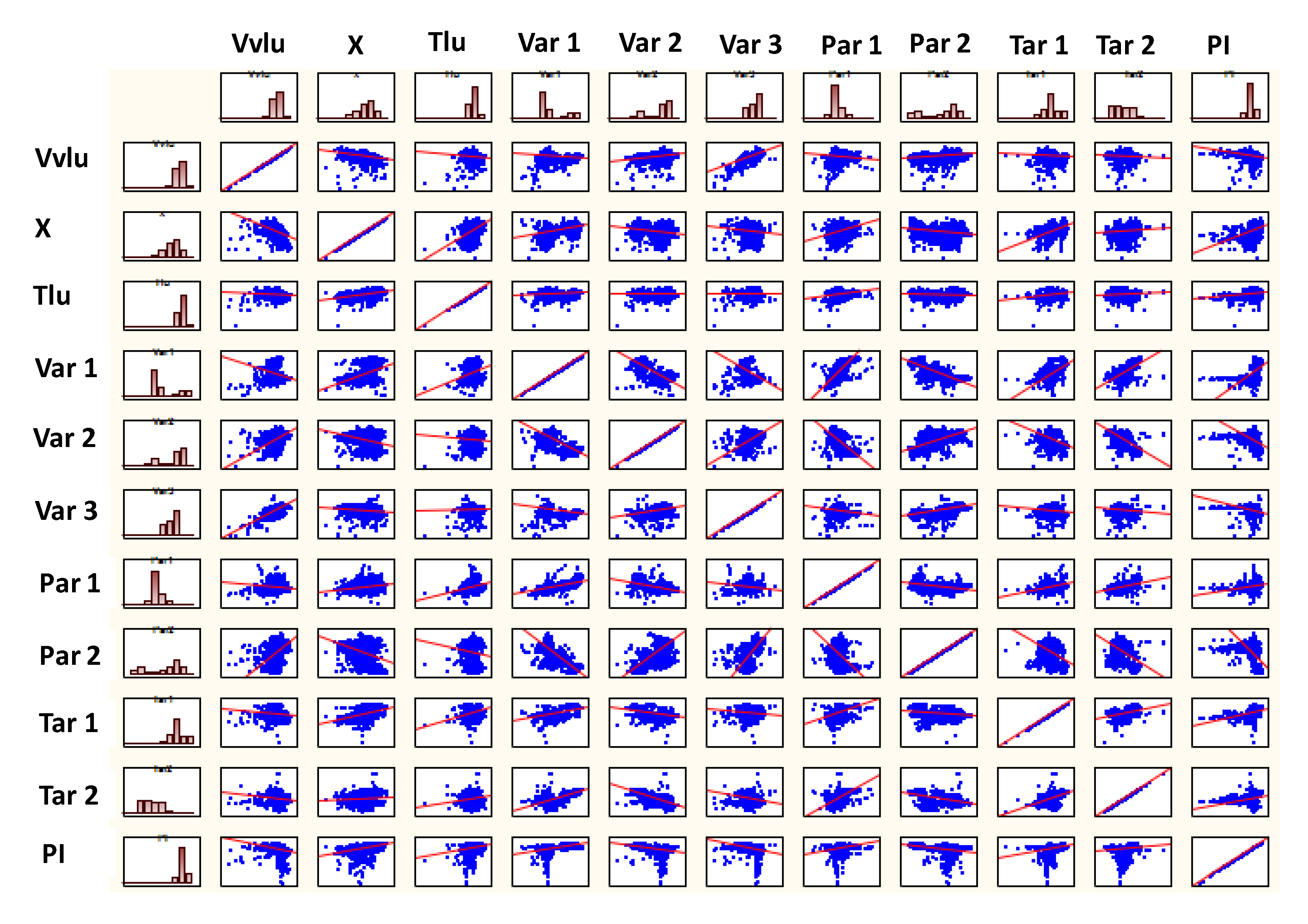
Discarding features with no importance for class discrimination does not guarantee that there is no variable redundancy. So, a correlation analysis was performed. Figure 7 shows the scatterplot matrix of the correlations between the input variables. Considering that none of the correlation coefficients is greater than 0.9, 11 process variables were used in the input layer of the FDD ANN model.

The model development algorithm had a total running time of 60 h of computational effort. The best ANN model—built with augmented data—has 11 neurons on the input layer, 27 neurons on the hidden layer, and 2 neurons on the output layer. The ANN model exhibits an overall performance index of 85.6%, an error rate of 19.6% for normal events, and 16.7% for fault events during the training phase.

In the model validation phase, the classifier was tested using a set of independent real process data cases. Its confusion matrix is shown in

Table 3. Artificial neural network (ANN) model confusion matrix (expanded data).

ANN Topology: RBFN 11-27-2	Class 1	Class 2	Overall
Total	3184.0	197.0	3381.0
Correct	2225.0	124.0	2349.0
Incorrect	959.0	73.0	1032.0
Correct (%)	69.9	62.9	69.5
Incorrect (%)	30.1	37.1	30.5

and the sensitivity and specificity values are, respectively, 0.63 and 0.70. The results showed that the overall classification error increases as the classification tool becomes more accurate in detecting faulty states, i.e., more sensitive. At the same time, the number of false alarms increases, i.e., the model becomes less specific. However, the classification risks associated with the losses of a false positive alarm (a normal operational condition diagnosed as fault) are smaller than the losses regarding false negative detections (missing an abnormal operation) and the consequent economical losses due to unplanned shutdowns.

It should be noticed that the variance of the error estimate is predominantly influenced by the size of the validation data set. A larger and proper selection of the raw process data set leads to a classification method with higher accuracy. Furthermore, real process data can be used in association with synthetic data in the training and validation phases by means of sample partition methodologies.

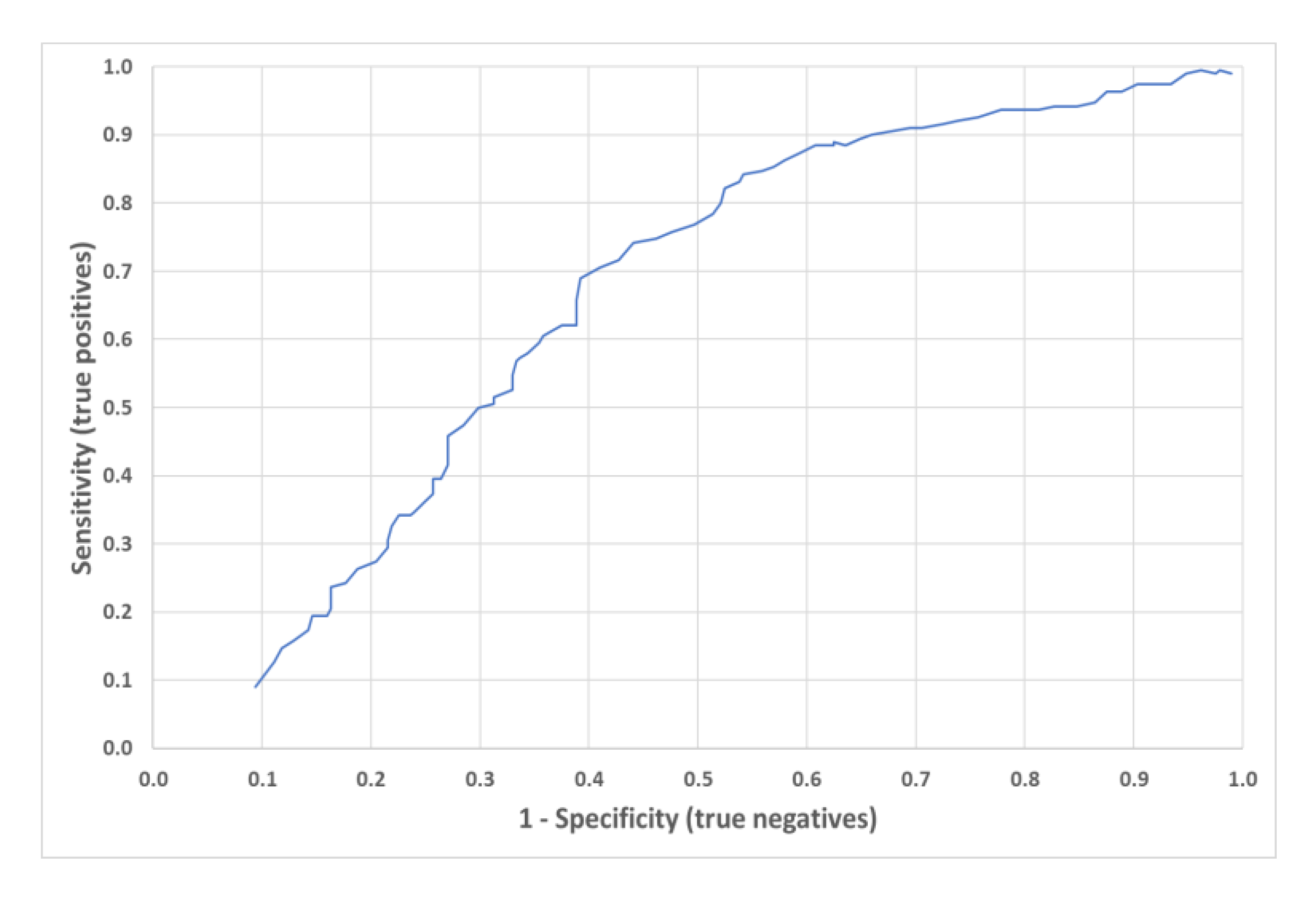
Figure 8 displays the ROC curve of the RBFN FDD model developed presenting an underlying area of 0.69 and a feature threshold of 0.52. The shape of the curve is off diagonal, inferring that the model is an informative classifier. Considering that the model is applied to a scenario where the prevalence of abnormal situations is low, and the classification tool would be expected to operate in the lower left part of the ROC curve (small threshold), in order to keep the false positive ratio (FPR) as small as possible. Given the high prevalence of normal scenarios, the high rate of false alarms obtained can be explained by the threshold value of the classifier of 0.52, an intermediate value. The high underlying curve area suggests that the classification method is robust because it performs well for a large range of prevalence situations.

Table 4. ANN model confusion matrix (real process data).

ANN Topology: RBFN 11-21-2	Class 1	Class 2	Overall
Total	2232.0	135.0	2367.0
Correct	2215.0	15.0	2230.0
Incorrect	17.0	120.0	137.0
Correct (%)	99.2	11.1	94.2
Incorrect (%)	0.8	88.9	5.8

was included for purposes of comparison between the classifier model developed with augmented data and the model built exclusively with raw process data, both following the same methodology for training and refinement. Regarding the proposed methodology in this work, the performance improvement of the developed model is clear. Although the network exclusively trained with real data has high overall performance, an inspection of the error rates for individual classes shows that this classifier tool is not able to diagnose fault operation and therefore would be of no use in a real application. This model will rarely detect an abnormal situation when it occurs, due to sensitivity values of 0.11. Nevertheless, the specificity value of 0.99 represents that if the classification tool identifies an abnormal situation, it will have a high probability of being a true positive scenario.

5. Conclusions

Predictive process fault detection and diagnosis (FDD) models—especially those based on machine learning techniques—are part of a growing effort to accomplish the automation of abnormal situation management. Nonetheless, real process data are typically unbalanced and majorly representative of normal process operation.

This work used the Monte Carlo technique to massively increase the amount of the original real data standards—a robust mathematical solution to deal with unbalanced data sets. In an innovative way, the methodology also used geometric distances and the nearest neighbors search to keep the original phenomenological characteristics of the original data set in the categorical augmented data collection. The simulation dismissed the need for experiments that could jeopardize process safety. In total, 160,000 artificial process cases were generated and a new uniformly distributed data collection of 5502 patterns was used to train a multilayered radial basis neural network, in order to classify the process operation within normal and failure events.

The RBFN FDD model developed was validated with real process plant data of a Brazilian pulp and paper mill, in order to monitor the formation of particles in a recovery boiler—a key equipment in kraft’s pulp and paper production plants. The FDD tool was able to correctly classify the normal and failures status in almost 70% of the cases, with a sensitivity of 0.63 and a specificity of 0.70. The ROC curve underlying area of about 0.7 suggests that it is a robust model for a wide range of class prevalence.

The data augmentation methodology embedded with the machine learning-based FDD model was compared with traditional FDD techniques and also with previous results reported in the literature [40,45] for this case study and outperformed them.