Short-Term Wind Power Prediction Based on Improved Grey Wolf Optimization Algorithm for Extreme Learning Machine

Abstract

In order to improve the accuracy of wind power prediction and ensure the effective utilization of wind energy, a short-term wind power prediction model based on variational mode decomposition (VMD) and an extreme learning machine (ELM) optimized by an improved grey wolf optimization (GWO) algorithm is proposed. The original wind power sequence is decomposed into series of modal components with different center frequencies by the VMD method and some new sequences are obtained by phase space reconstruction (PSR). Then, the ELM model is established for different new time series, and the improved GWO algorithm is used to optimize its parameters. Finally, the output results are weighted and merged as the final predicted value of wind power. The root-mean-square error (RMSE), mean absolute error (MAE), and mean absolute percentage error (MAPE) of the proposed VMD-improved GWO-ELM prediction model in the paper are 5.9113%, 4.6219%, and 13.01% respectively, which are better than these of ELM, back propagation (BP), and the improved GWO-ELM model. The simulation results show that the proposed model has higher prediction accuracy than other models in short-term wind power prediction.

1. Introduction

Over the past two decades, rising energy demand has driven the development of renewable energy. Wind energy, with its advantages of non-pollution and abundant reserves, has received worldwide attention and development [1]. However, due to the randomness of wind energy, there is no significant breakthrough in wind energy utilization. Therefore, it is particularly essential to predict wind power [2,3] for exploiting wind energy much more efficiently and reasonably. Wind power prediction is one of the most practicable methods.

Currently, there are two categories of wind power predictions approaches which are: the physical method [4] and the statistical method [5], according to different prediction models. The data of wind speed and direction measured by numerical weather forecast are employed as input data to realize the prediction of wind power [6], which is called the physical method. The measured data and historical data are used in the statistical method to establish the functional input-output relationship, which is used for wind power prediction. The statistical method is suitable for short-term wind power prediction.

By contrast, the extreme learning machine (ELM) has the advantages of fewer parameters, higher learning speed, and more excellent generalization performance [7]. However, how to determine the parameters of ELM is a challenging problem which has attracted many scholars from all over the world to focus on it. To solve these problems, the particle swarm optimization (PSO) algorithm was proposed to optimize the ELM parameters in Reference [8]. In Reference [9], the bat algorithm (BA) was used to optimize the parameters of ELM. These basic intelligent algorithms may still be improved in the aspects of local optimum and slow convergence speed.

In addition, some scholars have put forward several proposals to reduce the volatility of wind power prediction. For example, in References [10,11], wavelet decomposition was used to decompose the original sequence into sub-sequences with different frequency bands. In Reference [12], ensemble empirical mode decomposition (EEMD) was used to decompose the original sequence into different components with characteristic differences. The use of spatial correlation for the wind power prediction method was studied in Reference [13].

According to the current research status, this paper proposed an improved ELM model based on the variational mode decomposition (VMD) algorithm and the improved grey wolf optimization (GWO) algorithm. With the improved ELM, a short-term wind power prediction model was established. Firstly, the original wind power sequence was decomposed into several intrinsic modal components with different center frequencies by using the VMD algorithm to reduce the instability of the original wind power sequence. Then, modal components were autonomously combined into high-, medium-, and low-frequency waves according to the size of the sample entropy [14] value, and the prediction model based on ELM was established for each kind of wave, respectively. Moreover, the improved GWO algorithm was employed to optimize the parameters of the ELM, which are input weight and hidden layer bias of the standard ELM. The sum of the absolute value generated by the prediction was set as the optimization fitness function for the improved GWO algorithm. Finally, the predicted values of each component were weighed and reconstructed to obtain the actual predicted results. By applying the model proposed in this paper, the short-term wind power prediction was carried out with the actual wind power data, and the final simulation results proved that the proposed model is more feasible and effective. The innovations of this paper are as follows:

• The GWO algorithm is improved. Firstly, the nonlinear convergence factor is proposed to improve the convergence precision of the algorithm. Then, the beetle antennae search (BAS) algorithm is used to optimize the GWO algorithm, which increases the environment judgement ability for the beetle individuals and avoids the algorithm falling into the local optimum.
• VMD is used to decompose the original wind power sequence. Firstly, the modal components generated by decomposition of the original wind power sequence by the VMD algorithm are autonomously combined into a low-frequency wave, medium-frequency wave, and high-frequency wave respectively, according to the size of the sample entropy value. Moreover, the reconstructed waveforms are respectively predicted by the improved GWO-ELM. Finally, the results are merged into the final prediction results.
• Four classical test functions are used to test the optimization ability of the PSO and GWO algorithms, respectively. By comparing the test results, it is found that the improved GWO algorithm can increase the optimization speed of the algorithm and avoid the algorithm falling into local optimum. By comparison with ELM, BP, and the improved GWO-ELM, it shows that the model proposed in this paper has a better prediction effect.

The structure of this paper is organized as follows: In Section 2, two improvements of the GWO algorithm are proposed. The first one is the thought of the linear convergence factor and the other is the combination of the beetle antennae search algorithm and the standard GWO algorithm. In Section 3, several ELM prediction models are established by using the modal components obtained by VMD, and the model parameters are optimized by the improved GWO algorithm. In Section 4, with the actual wind power data, several simulations have been implemented to verify the optimization performance of the improved GWO algorithm and prediction model. Finally, Section 5 summarizes this paper.

2. Improved Grey Wolf Optimization Algorithm

2.1. Standard Grey Wolf Optimization Algorithm

The grey wolf optimization (GWO) algorithm [15,16], which simulates the hierarchy and predation behavior of wolves, is one sort of swarm intelligence algorithm. Its evident strengths are a simple mechanism, few parameters, and easy implementation. The algorithm separates the entire wolf group into four layers. The first layer is the alpha wolf ($\mathsf{\alpha }$) who is responsible for making decisions about predation, habitat, and schedule. Other wolves must obey the command from the alpha wolf ($\mathsf{\alpha }$). The second layer is the beta wolf ($\mathsf{\beta }$), who obeys and assists the $\mathsf{\alpha }$. The third layer is the delta wolf (δ), who obeys the α and the β while dominating the rest of the wolf group. The fourth layer is the omega wolf ($\mathsf{\omega }$), who must obey other social-level wolves. The former three layers have the best fitness values and lead the group towards the target. Its hunting process mainly includes: tracking, encircling, and attacking.

• Tracking process: When the grey wolf searches for prey, it gradually approaches the prey and surrounds it. The distance between the grey wolf and the prey during the tracking process is:

  $$\{\begin{array}{l}D=|C·{\mathrm{X}}_{\mathrm{P}}(t)-\mathrm{X}(t)|\\ \mathrm{X}(t+1)={\mathrm{X}}_{\mathrm{p}}(t)-A·D\end{array}$$

  (1)

  where $D$ is the distance between the grey wolf and the prey, $t$ is the current number of iterations, ${\mathrm{X}}_{\mathrm{P}}(t)$ is the position of the prey after the t-th iteration (i.e., the position of the optimal solution), $\mathrm{X}(t)$ is the position of the grey wolf after the t-th iteration (i.e., the locations of the potential solution), $A$ and $C$ are the coefficient factor, and its calculation equation is:

  $$\{\begin{array}{l}A=2a·r_1-a\\ C=2·r_2\end{array}$$

  (2)

  $$a=2-2(\frac{t}{T})$$

  (3)

  where $r_1$ and $r_2$ are the random numbers limited from 0 to 1, and $a$ decreases linearly from 2 to 0 as the number of iterations increases.
• Encircling process: The grey wolf can identify the location of the potential prey (optimal solution). The encircling process is mainly done by the guidelines of α, β, and δ. It normally assumes that α, β, and δ have a strong ability to identify the positions of potential prey. During each iteration, the best three grey wolves, α, β, and δ, from the current population are retained. Finally, the positions of ω are updated by their location information.

  $$\{\begin{array}{l}{D}_{\mathsf{\alpha }}=|C_1·{\mathrm{X}}_{\mathsf{\alpha }}(t)-\mathrm{X}(t)|\\ D_{\mathsf{\beta }}=|C_2·{\mathrm{X}}_{\mathsf{\beta }}(t)-\mathrm{X}(t)|\\ D_{\mathsf{\delta }}=|C_3·{\mathrm{X}}_{\mathsf{\delta }}(t)-\mathrm{X}(t)|\end{array}$$

  (4)

  $$\{\begin{array}{l}{\mathrm{X}}_1={\mathrm{X}}_{\mathsf{\alpha }}(t)-A_1{D}_{\mathsf{\alpha }}\\ {\mathrm{X}}_2={\mathrm{X}}_{\mathsf{\beta }}(t)-A_2{D}_{\mathsf{\beta }}\\ {\mathrm{X}}_3={\mathrm{X}}_{\mathsf{\delta }}(t)-A_3{D}_{\mathsf{\delta }}\end{array}$$

  (5)

  where $D_{\mathsf{\alpha }}$, $D_{\mathsf{\beta }}$, and $D_{\mathsf{\delta }}$ are the distances between $\mathsf{\alpha }$, $\mathsf{\beta }$, $\mathsf{\delta }$ wolves and $\mathsf{\omega }$ wolves. ${\mathrm{X}}_{\mathsf{\alpha }}$, ${\mathrm{X}}_{\mathsf{\beta }}$, and ${\mathrm{X}}_{\mathsf{\delta }}$ represent the positions of $\mathsf{\alpha }$, $\mathsf{\beta }$, and $\mathsf{\delta }$ in the current population. ${\mathrm{X}}_1$, ${\mathrm{X}}_2$, and ${\mathrm{X}}_3$ are the moving step size and directions of the $\mathsf{\omega }$ wolves toward $\mathsf{\alpha }$, $\mathsf{\beta }$, and $\mathsf{\delta }$, respectively.
• Attacking process: When the artificial wolves surround the prey, they are going to start hunting. Their positions are mainly updated by $\mathsf{\alpha }$, $\mathsf{\beta }$, and $\mathsf{\delta }$ wolves.

  $$\mathrm{X}(t+1)=\frac{{\mathrm{X}}_1{+\mathrm{X}}_2{+\mathrm{X}}_3}{3}$$

  (6)

  where $\mathrm{X}(t+1)$ is the calculated position of the updated $\mathsf{\omega }$ wolves. In combination with Equation (2), $A$ changes as $a$ changes. When $|A|>1$, the grey wolves spread out in each area as far as possible to search for prey. Hence, the algorithm expands its search area. When $|A|<1$, the grey wolves focus on one or more particular areas of prey, which results in a decrease of the search scope of the algorithm.

There may still be some problems with the standard GWO algorithm. Firstly, the convergence factor in the standard GWO decreases linearly from 2 to 0 with the increasing numbers of iteration. During this procedure, the exploration and development process of GWO is not fully reflected, which leads to the low convergence accuracy. Secondly, the standard GWO algorithm focuses on the influence of the group on individuals and ignores the judgment of the individuals in the attacking process. Consequently, it is easy to fall into local optimum. Based on the analysis, these issues will be addressed separately.

2.2. Nonlinear Convergence Factor

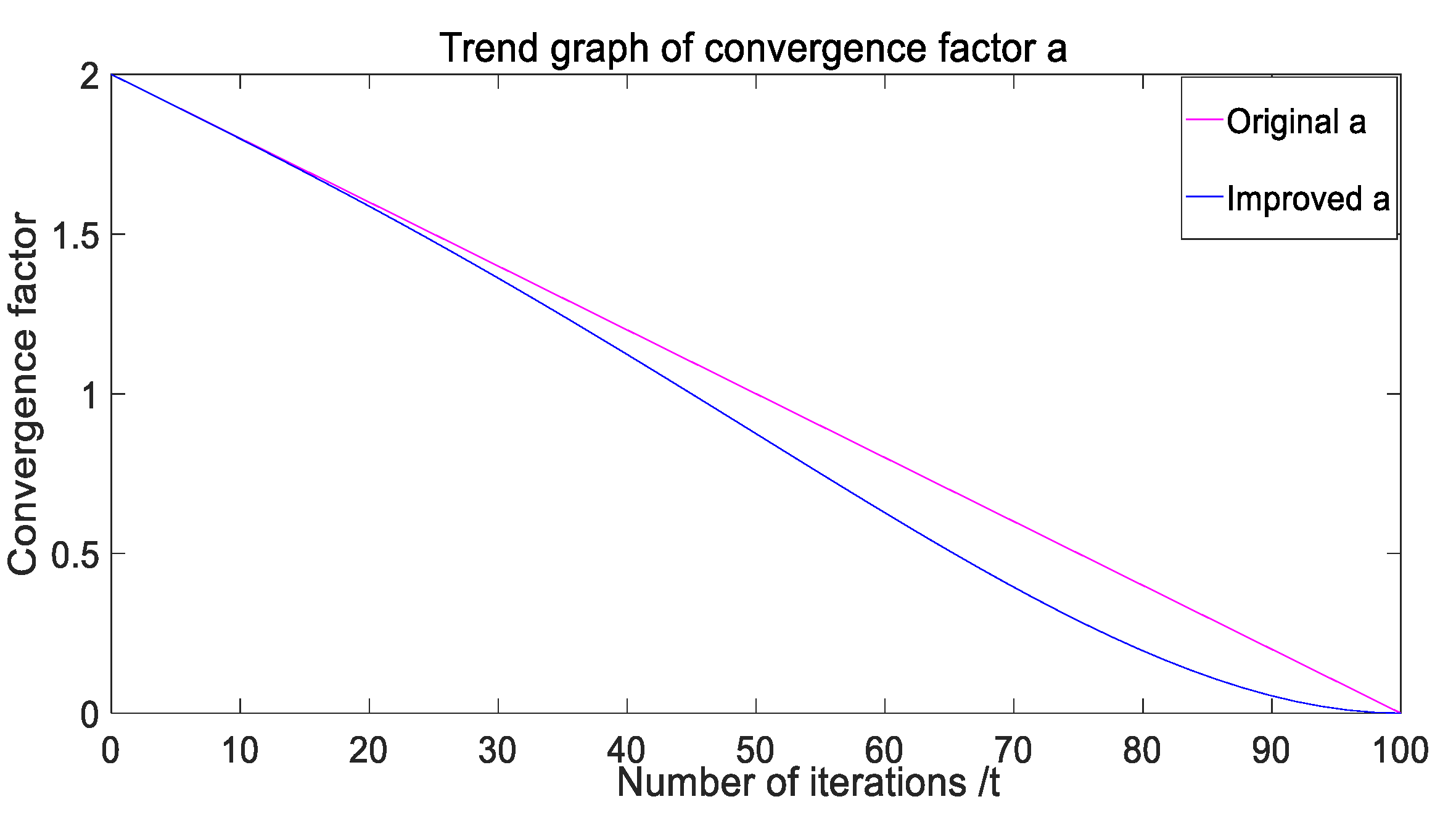
The nonlinear convergence factor $a$ is proposed for the problem of low convergence precision of the GWO algorithm, which determines the global search and local search performance of the GWO algorithm. The larger the $a$, the greater the global search capability. The smaller the $a$, the stronger the local development capability [17]. The nonlinear convergence factor $a$ can be expressed as:

$$a=(2-\frac{2t}{T_{max}})(1-\frac{t^3}{T_{max}^3})$$

(7)

where $t$ is the current number of iterations and $T_{max}$ is the maximum number of iterations.

The comparison of original and improved a is displayed in Figure 1. The convergence factor of improved a nonlinearly decreases from 2 to 0. As the number of iterations increases, the decay rate of the convergence factor gradually decreases, which enhances the local search ability and the local optimal solution is more accurate. Therefore, this nonlinear convergence factor is more consistent with the actual convergence process of the algorithm, which can better balance the global search and local search performance of the algorithm and avoid the algorithm falling into local optimum.

2.3. Improved GWO Algorithm Based on the Beetle Antennae Search Algorithm

The beetle antennae search (BAS) algorithm [18,19,20] is an efficient, intelligent optimization algorithm proposed in 2017. Beetles search for food according to the intensity of food odor. If the odor intensity received by the right antenna is larger than that on the left, beetles will fly to the right. Otherwise, they will fly to the left. The intensity of food odor felt by beetles at each point is the value of fitness function. The purpose of its flight is to find the position where the intensity of food odor is strongest.

The BAS algorithm is similar to other optimization algorithms, like the ant colony optimization (ACO) algorithm [21], the particle swarm optimization (PSO) algorithm [22], the cuckoo search optimization (CSO) algorithm [23], etc. However, it can intelligently and efficiently search without knowing the specific form and gradient information of the function.

The specific algorithm flow is as follows:

• Randomly initialize the position, $x$, of the beetle, and the distances between the two antennas of each beetle are $d_0$;
• Calculate the fitness value of the beetle $f(x)$;
• Randomly generate the direction of the antennas according to Formula (8), and update the step according to Formula (9):

  $$\overrightarrow{b}=\frac{\mathrm{rnd}(D,1)}{||\mathrm{rnd}(D,1)||}$$

  (8)

  $${\mathsf{\delta }}^t=k{\mathsf{\delta }}^{t-1}$$

  (9)

  where $\mathrm{rnd}$ is a random function, $D$ is the spatial dimension, $k$ is the decay factor of the step size, and ${\mathsf{\delta }}^t$ is the search step of the beetle at time $t$.
• Determine the positions of the left and right antennas according to Formula (10):

  $$x_l=x^t-d^t\overrightarrow{b}$$

  (10)

  $$x_r=x^t+d^t\overrightarrow{b}$$

  (11)

  where $x_l$ and $x_r$ are positions of the beetle’s left and right antennas, $x^t$ is the position of the beetle’s center of mass at time $t$, and $d^t$ is the distance between the two antennas at time $t$. In practice, adjustments can be made according to the step size, specifically as in Formula (12):

  $$d^t=\frac{{\mathsf{\delta }}^t}{c}$$

  (12)

  where $c$ is a constant, $c\in$ [2, 10].
• Calculate the fitness value $f(x_l)$ and $f(x_r)$ of the left and right antennae.
• Determine the direction of the next movement of the beetle, and further update the position according to a combination of Formula (13) and the fitness values of left and right antennas:

  $${\mathrm{x}}^{t+1}={\mathrm{x}}^t+{\mathsf{\delta }}^{t+1}\overrightarrow{b}\mathrm{sign}(f(x_r)-f(x_l))$$

  (13)
• Judge whether the convergence condition is met, namely, the maximum number of iteration or the set precision. If so, the iteration is terminated. Otherwise, continue the iteration process from step 3.

Compared with the PSO algorithm, ACO algorithm, CSO algorithm, and other algorithms, the BAS algorithm only needs the individual to search optimal solution. Besides, its computational cost is low, the process is simple, and implementation is easy. Therefore, it is appropriate to combine the advantages of the BAS algorithm and GWO algorithm to solve the problem that the GWO algorithm focuses too much on the group. Consequently, the GWO algorithm optimized by the BAS algorithm is proposed. The main ideas are as follows:

Firstly, according to the idea of the BAS algorithm, the α, β, δ, and a random grey wolf among the wolves group are described as the elite individuals. In the iterative process, the position update of the wolf group not only solely relies on the guidance of three such kinds of wolves, but also relies on the judgment of the environment from the elite grey wolves in each iteration. Thus, it prevents the GWO algorithm from falling into local optimum.

Then, elite individuals compare the fitness function values of the left and right sides during each iteration. The optimal value can be obtained for updating the position of the grey wolf group.

By constructing the elite grey wolf individuals mentioned previously, it is efficient to overcome the poor stability caused by the GWO algorithm and the problem of local optimum.

The flow of the improved GWO algorithm is as follows:

• Initialize the number of wolf group, $N$, dimension, $D$, number of iteration, $m$, and wolf group, ${\mathrm{X} = [\mathrm{X}}_1{,\mathrm{X}}_2,\dots {,\mathrm{X}}_{\mathrm{N}}]$ of the GWO algorithm.
• Calculate the fitness value of the grey wolf individual.
• Select α, β, and δ according to the size of the fitness value.
• Define α, β, δ, and a wolf randomly selected in the wolf group as beetles. Calculate position $x$ and fitness function value $f(x)$ of the left and right antennae for each beetle. Compare the fitness function of each grey wolvf and select the final α, β, and δ.
• Update the position of the ordinary wolf, $\mathsf{\omega }$, according to the position iteration equation.
• Update parameters $a,A,C$.
• Judge whether the stop condition is satisfied, otherwise move to the second step.
• Output the position and fitness value of the α wolf.

3. Short-Term Wind Power Prediction Model

3.1. Standard Extreme Learning Machine

Standard intelligent learning algorithms, such as the neural network algorithm [24], usually adopt the gradient descent method to adjust weight parameters. However, this may cause algorithms to slow down learning speed and fall into the local minimum. According to these problems, Huang et al. proposed the method of the extreme learning machine (ELM) [25]. ELM reduces the calculation of model parameter selection while preserving the generalization of the neural network.

The main ideas are as follows:

Input n samples $\mathrm{X}=\left\{x_1,x_2,x_3,\cdots x_n\right\}$, one of the outputs among the samples is:

$$y_j={\displaystyle \sum _{i=1}^l{\mathsf{\beta }}_{i}g(w_i\cdot x_j+b_i)}$$

(14)

where ${\mathsf{\beta }}_i$ is the output weight, $g(·)$ is the activation function, $w_i$ is the input weight, $b_i$ is the hidden layer bias, and $w_i\cdot x_j$ is the inner product of $w_i$ and $x_j$.

Then, the model is trained to minimize the error. It normally assumes that the error is 0, which means the existence of ${\mathsf{\beta }}_i$, $w_i$, and $x_j$ makes the training result equal to the output result.

The specific equation is as follows:

$$Y=\mathsf{\beta }H$$

(15)

where

$$\mathsf{\beta }=\left\{{\mathsf{\beta }}_1, {\mathsf{\beta }}_2, {\mathsf{\beta }}_3\cdots {\mathsf{\beta }}_l\right\}$$

(16)

$$Y=\left\{y_1,y_2,y_3,\cdots ,y_l\right\}$$

(17)

$$H=\left(\begin{array}{ccc}g(w_1\cdot x_1+b_1)& \cdots & g(w_1\cdot x_n+b_1)\\ \cdots & \cdots & \cdots \\ g(w_l\cdot x_1+b_l)& \cdots & g(w_l\cdot x_n+b_l)\end{array}\right)$$

(18)

Solving $\min {\Vert H\mathsf{\beta }-Y\Vert }^2$, where $Y$ is the actual output, $H$ is determined by $b_i$ and $w_i$ which are set randomly. Finally, the $\mathsf{\beta }$ is solved to bulid the model.

3.2. Optimized ELM based on VMD

The standard ELM has some distinct advantages. Nevertheless, there are still some problems with it, which will cause the inefficient prediction effect of the eventual wind power model if the actual wind power data are directly used to train the limit learning machine due to its violent fluctuation and randomness.

For this reason, variational mode decomposition (VMD) is used to decompose the original wind power sequence in priority. VMD [26] is a new signal decomposition estimation method proposed by Dragomiretskiy et al. in 2014, and its overall framework is a variational problem.

VMD decomposes the input signal into several sub-modes to minimize the sum of the estimated bandwidths of each mode [27]. It normally assumes that each mode is limited bandwidth with a different center frequency. Then, by alternating the direction multiplier method, each mode and center frequency is updated continuously. As a result, each of the modes gradually demodulates to their corresponding fundamental frequency bands. Finally, each of the modes and corresponding center frequencies are extracted.

The process of the VMD algorithm is as follows:

• For each mode function $u_k(t)$, the analytic signal is obtained through Hilbert transformation for obtaining the one-sided spectrum.

  $$[\mathsf{\delta }(t)+\frac{j}{\pi t}]\ast u_k(t)$$

  (19)

  where $\mathsf{\delta }(t)$ is the unit pulse function.
• Estimate the center frequency of each modal function by adjusting the exponent $e^{-j{w}_{k}t}$, and then modulate the spectrum of each mode to the corresponding baseband.

  $$[(\mathsf{\delta }(t)+\frac{j}{\pi t})\ast u_k(t)]e^{-j{w}_{k}t}$$

  (20)
• Construct a constrained variational problem of Equation (21) by calculating the square of the $L2$-norm of the demodulated signal gradient.

  $$\underset{\left\{u_k\right\}\left\{w_k\right\}}{\min }\{{\displaystyle \sum _{k=1}^K||{\partial }_t[(\mathsf{\delta }(t)+\frac{j}{\pi t})\ast u_k(t)]e^{-j{w}_{k}t}}|{|}^2\}$$

  (21)

  It also meets the following condition:

  $${\displaystyle \sum _{k=1}^K{u}_k=f}$$

  (22)

  where $f$ is a time series, $u_k$ is a mode signal, $k$ is the number of modes, * presents the convolution, and $w_k$ indicates the center frequency of the kth mode.

After that, the phase space reconstruction (PSR) [28,29] is carried out for the above decomposition waveforms, respectively. The idea of PSR is as follows:

For the original sequence, $\mathrm{X}(t)=[x_1,x_2,\cdots ,x_n]$, the reconstructed phase space sequence is shown in Equation (23):

$$\begin{array}{c}\mathrm{X}(1)=\left\{x(1),x(1+\mathsf{\tau }),\cdots ,x(1+(m-1)\mathsf{\tau })\right\}\hfill \\ \mathrm{X}(2)=\left\{x(2),x(2+\mathsf{\tau }),\cdots ,x(2+(m-1)\mathsf{\tau })\right\}\hfill \\ ⋮\\ \mathrm{X}(k)=\left\{x(k),x(k+\mathsf{\tau }),\cdots ,x(k+(m-1)\mathsf{\tau })\right\}\hfill \end{array}$$

(23)

where $\mathsf{\tau }$ is the delay time and $m$ is the embedded dimension.

3.3. Short-Term Wind Power Model based on the VMD-Improved GWO-ELM

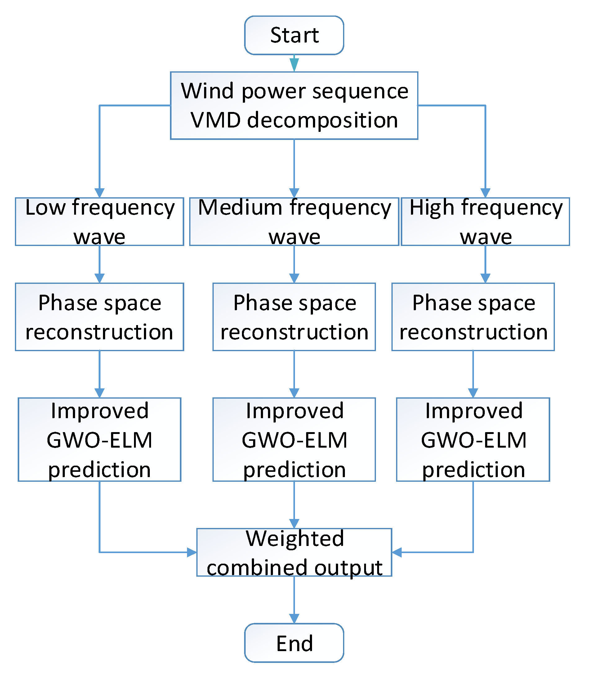
For further explaining the main sources of prediction error, the VMD algorithm was used to decompose the original wind power sequence into a series of modal components sequences and then autonomously combine them into high-, medium-, and low-frequency waves according to the size of its sample entropy value. Moreover, improved GWO-ELM prediction is conducted for each reconstructed waveform. Then, phase space reconstruction was carried out for the three kinds of waveforms, and the improved GWO-ELM prediction was implemented for the reconstructed sequence. Finally, the final output results were obtained by weighting the predicted results of the three models.

The specific process is shown in Figure 2.

4. Simulation Analysis

4.1. Improved GWO Algorithm Performance Verification

Randomly generating the input weight and hidden layer bias of the standard ELM will lead to its unstable performance and weak generalization ability. So, the improved GWO algorithm was used to optimize the initial parameters of the ELM in this paper.

Four classical test functions were selected to verify its effectiveness, convergence speed, and accuracy. The four functions are all multi-peak functions, which can be used to detect the ability of local searching and the ability to escape from local optimum. The expressions, variable ranges, and theoretical optimal values of each test function are shown in

Table 1. Classic test function experimental parameters.

Function	Expression	Variable Range	Theoretical Optimal Value
Ackley	$f_1=-20\exp (-0.2\sqrt{{\displaystyle \sum _{i=1}^n{x}_i{}^2/n}})-\exp ({\displaystyle \sum _{i=1}^n\cos (2\pi x_i)/n})+20+e$	[−32, 32]	0
Griewank	$f_2=\frac{1}{4000}{\displaystyle \sum _{i=1}^n{x}_i^2}-\prod \cos (\frac{x_i}{\sqrt{i}})+1$	[−600, 600]	0
Schaffer	$f_3=0.5+\frac{{(\sin \sqrt{x_1^2+x_2^2})}^2-0.5}{{(1+0.001(x_1^2+x_2^2))}_{}^2}$	[−10, 10]	−1
Shubert	$f_4=({\displaystyle \sum _{i=1}^{5}i\cos [(i+1)x+i]})\times ({\displaystyle \sum _{i=1}^{5}i\cos [(i+1)y+i]})$	[−10, 10]	−186.7309

.

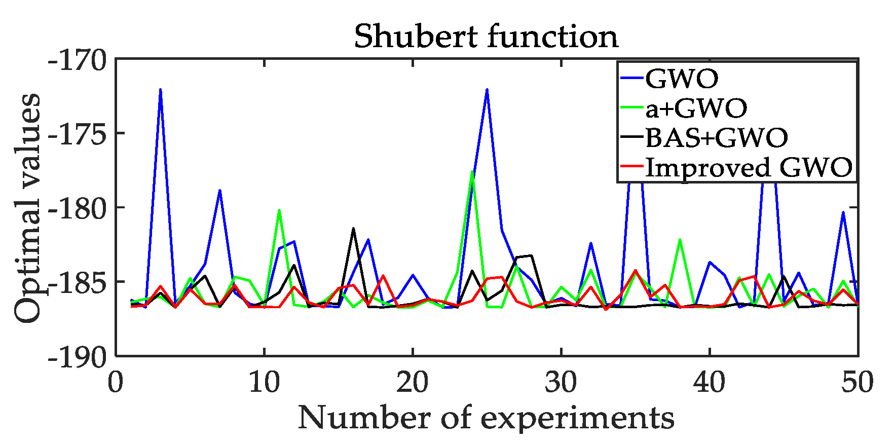
To verify the performance of the improved GWO algorithm proposed in this paper, the Shubert function in Table 1 has been respectively optimized by the standard GWO algorithm, the GWO algorithm improved by the nonlinear convergence factor (a + GWO), the GWO algorithm combined with BAS algorithm (BAS + GWO), and the GWO algorithm improved by both of the improvements. The method of the test is that conducting 50 independent experiments, with 200 times cycle number for each experiment, and the population is 20.

Figure 3 shows the convergence curve of Shubert optimization using four algorithms. It is obvious that both the nonlinear convergence factor and the improvement combined with the BAS algorithm can increase the optimization effect of the GWO algorithm. However, the convergence effect of the BAS + GWO algorithm is much better. Meanwhile, the variance of the BAS + GWO algorithm is 1.2541, which is smaller than 3.03569 of the a + GWO algorithm. In comparison of the optimization results’ mean value −185.671 of the a + GWO algorithm, the same value of the BAS + GWO algorithm is −186.0797, which is closer to the theoretical optimal solution −186.7309. It further indicates that both improvements of nonlinear convergence factor and the combination with the BAS algorithm can increase the optimization effect of the algorithm, among which, the latter one improves the GWO algorithm better. Therefore, the combination of two improvements can better optimize the performance of the GWO algorithm.

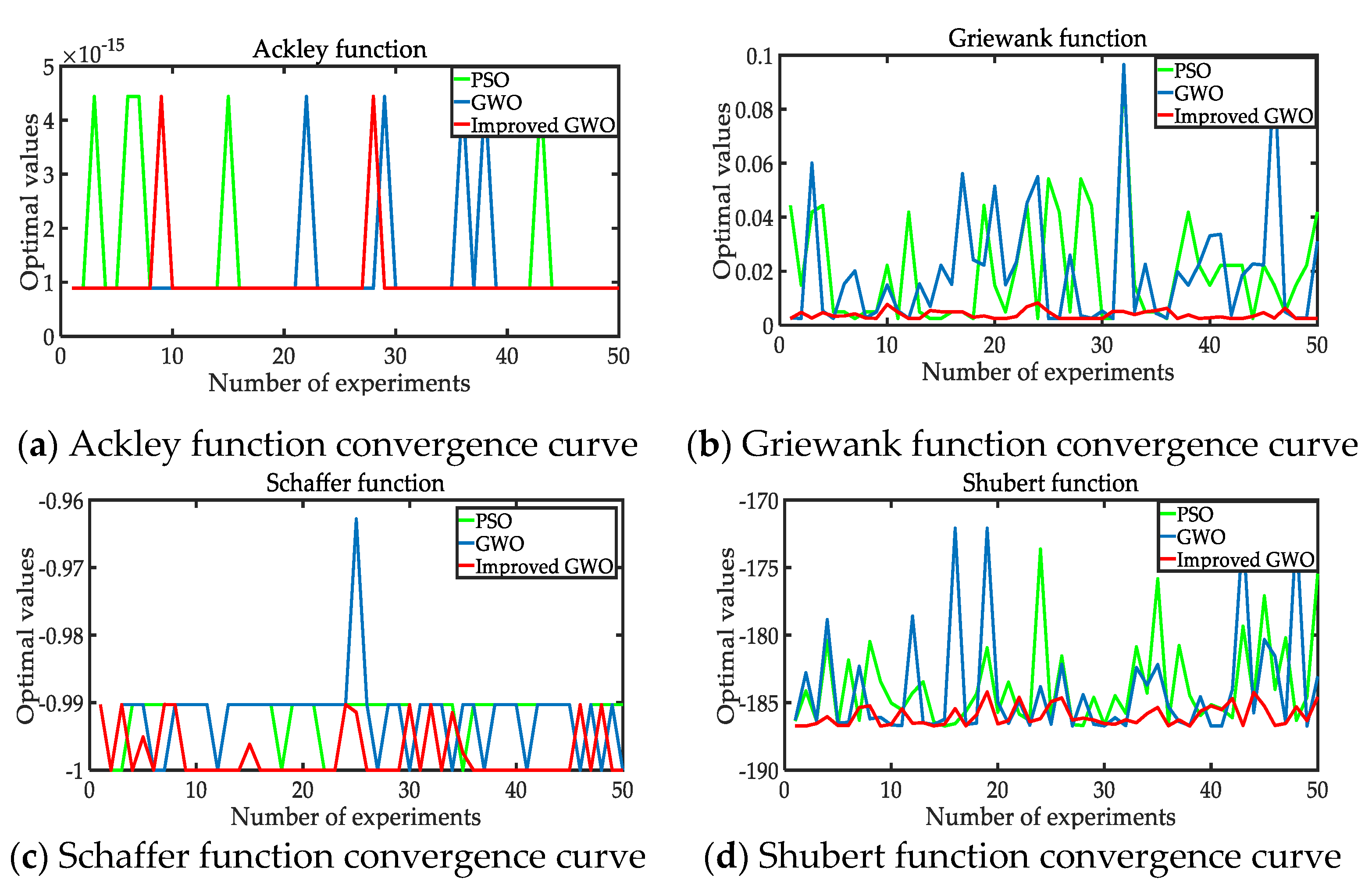
Furthermore, with the same method of the above test, the standard PSO algorithm and the standard GWO algorithm were respectively used to optimize four classic test functions in Table 1, and the results were compared. It demonstrated the actual performance of the improved GWO algorithm.

(a), (b), (c), and (d) of Figure 4 are the convergence curves of each function under the standard PSO algorithm, standard GWO algorithm, and improved GWO algorithm, respectively. In Figure 4, compared to the prediction results of the three algorithms, the results of the improved GWO algorithm has the minimum times of deviating from the optimal solution and the smallest amplitude. It demonstrated that the improved GWO algorithm has better optimization accuracy and is more suitable for optimizing the initial parameters of the ELM model.

In order to further prove the convergence characteristics of the improved GWO algorithm, the optimal value, the worst value, the variance and the excellent rate of the results were compared, and the results are shown in

Table 2. Comparison of the three algorithms.

Function	Algorithm	Optimal Value	Worst Value	Variance	Excellent Rate
$f_1$	particle swarm optimization (PSO)	8.88 × 10−16	4.44 × 10−15	1.55 × 10−30	100%
	grey wolf optimization (GWO)	8.88 × 10−16	4.44 × 10−15	9.48 × 10−31	100%
	Improved GWO	8.88 × 10−16	4.44 × 10−15	4.95 × 10−31	100%
$f_2$	PSO	0.0025	0.0937	3.90 × 10−4	20%
	GWO	0.0025	0.0966	4.85 × 10−3	24%
	Improved GWO	0.0025	0.0082	2.35 × 10−6	46%
$f_3$	PSO	−1	−0.9903	1.42 × 10−5	18%
	GWO	−1	−0.9628	3.53 × 10−5	24%
	Improved GWO	−1	−0.9903	1.58 × 10−5	72%
$f_4$	PSO	−186.7255	−173.6157	10.4646	48%
	GWO	−186.7308	−172.0774	17.1044	58%
	Improved GWO	−186.7308	−184.1958	0.5803	86%

.

In Table 2, it should be noted that the excellent rates of the three algorithms for $f_1$ are 100%, and that for $f_2$, $f_3$, and $f_4$ are different, among which the improved GWO algorithm is the best one. Furthermore, it can prove that the improved GWO algorithm is more stable due to its smallest variance among the optimization results of the three algorithms in 50 independent experiments. In conclusion, the optimization result of the improved GWO algorithm is the best one, which indicates that the accuracy of the GWO algorithm can be optimized by the proposed method in this paper.

In summary, the optimal solution can be obtained more quickly and accurately with the improved GWO algorithm, and it is not easy to fall into the local optimum value during the implementation process.

4.2. Case Analysis

Figure 5 is the picture of 100 kw medium size wind turbines from a wind field in Henan, China. In this sector, a simulation experiment with the measured wind power data from Henan wind field have been carried out to verify the performance of the proposed short-term wind power prediction model. The 720 groups of data were selected to build the prediction model, and the sampling interval of wind power data was 15 min. Among these data, the former 624 data were used as training samples, and the rest of the 96 data were used as test samples.

4.2.1. Simulation Process

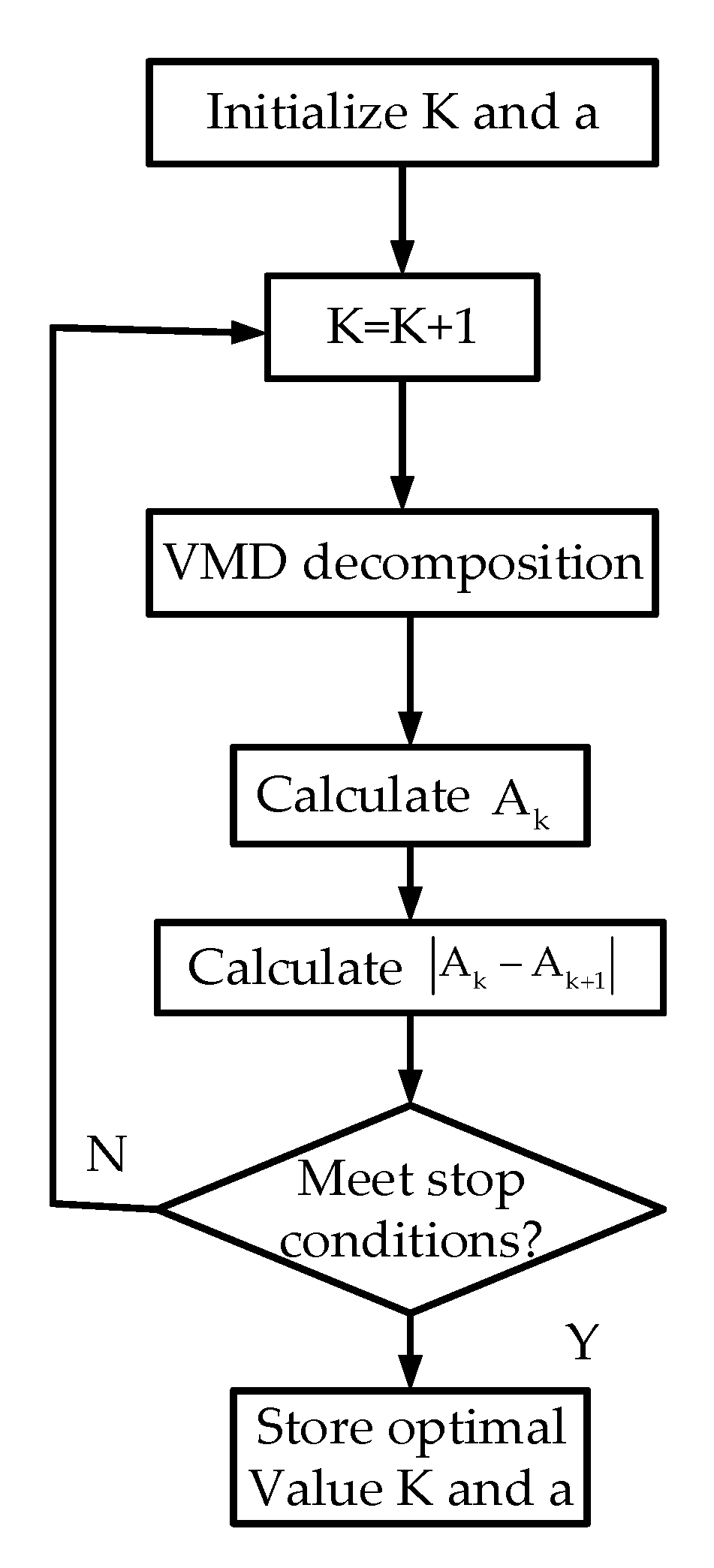
The number of decomposition mode number K is determined automatically by the method in Reference [30]. VMD decomposition is performed on the signal, and the correlation coefficient between the last modal component and the decomposition of the original signal is calculated. Firstly, suppose the modal number of VMD decomposition is k, and the correlation coefficient between the decomposition of the last modal component and the original signal is ${\mathrm{A}}_{\mathrm{k}}$. Then, if the decomposition of the modal number is k + 1, the corresponding value is ${\mathrm{A}}_{\mathrm{k}+1}$. When the difference between ${\mathrm{A}}_{\mathrm{k}}$ and ${\mathrm{A}}_{\mathrm{k}+1}$ is less than the threshold value a (a is set as 0.3% in this experiment), stop the decomposition. Otherwise, increase the value of k and keep decomposing until the stop condition is satisfied. Finally, record the final decomposition modal number k. The flow chart of VMD is as Figure 6:

Through the simulation experiment, when the value of k is in the range from 1 to 8, the minimum value among the 8 values of the $|{\mathrm{A}}_{\mathrm{K}}-{\mathrm{A}}_{\mathrm{K}+1}|$ is 0.5%, which is greater than a. When k = 9, the value of $|{\mathrm{A}}_{\mathrm{K}}-{\mathrm{A}}_{\mathrm{K}+1}|$ is 0.09%, which is less than a. Hence, k = 9.

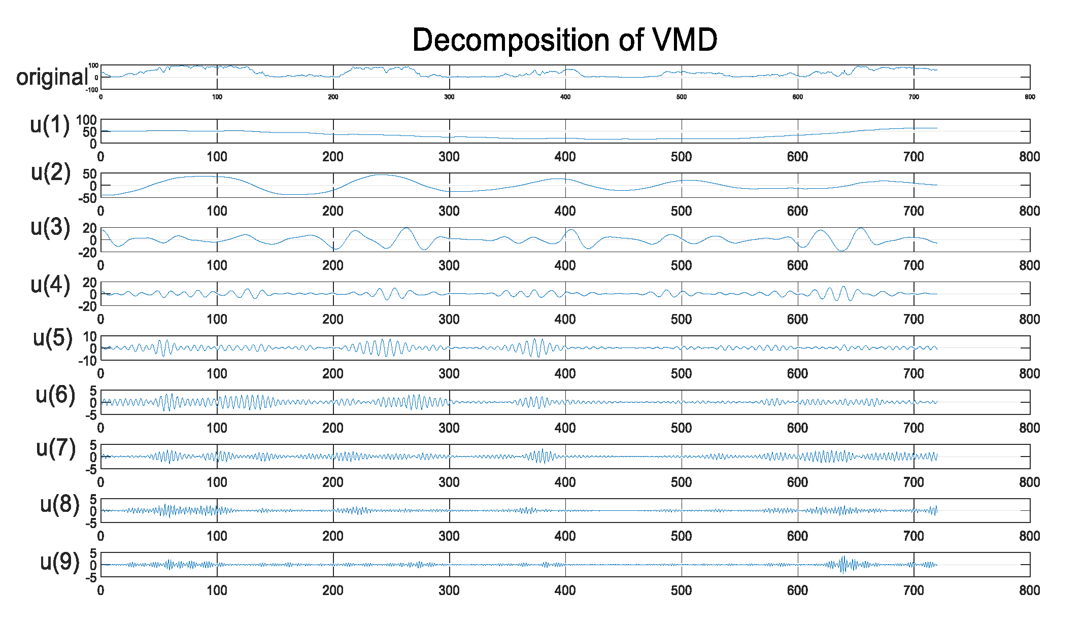
The decomposition result is shown in Figure 7, which shows the original wind power sequences diagram and series decomposed by VMD. By analyzing the original sequence, it is worth noting that the original wind power sequence has the characteristics of randomness and strong fluctuation, which will affect the accuracy of the prediction if it is directly used as the input of the prediction model. Hence, it is necessary to decompose the original wind power sequence through the VMD to improve the prediction accuracy of the model.

According to how close the sample entropy value is, the modal components are autonomously decomposed into high-frequency, medium-frequency, and low-frequency. In this paper, they are u(1)~u(2), u(3)~u(7) and u(8)~u(9), respectively.

Phase space reconstruction (PSR) was carried out for three different waveforms respectively, and input and output variables of the prediction model were set.

Finally, the improved GWO algorithm was used to optimize the initial parameters of the ELM model, and the sum of the absolute value of the training data output error of the ELM model was set as the fitness function. The improved GWO-ELM model was used to predict the three different frequency waveforms, respectively. Then, the prediction results of three waveforms were weighted and combined to obtain the final wind power prediction.

4.2.2. The Analysis of Simulation Results

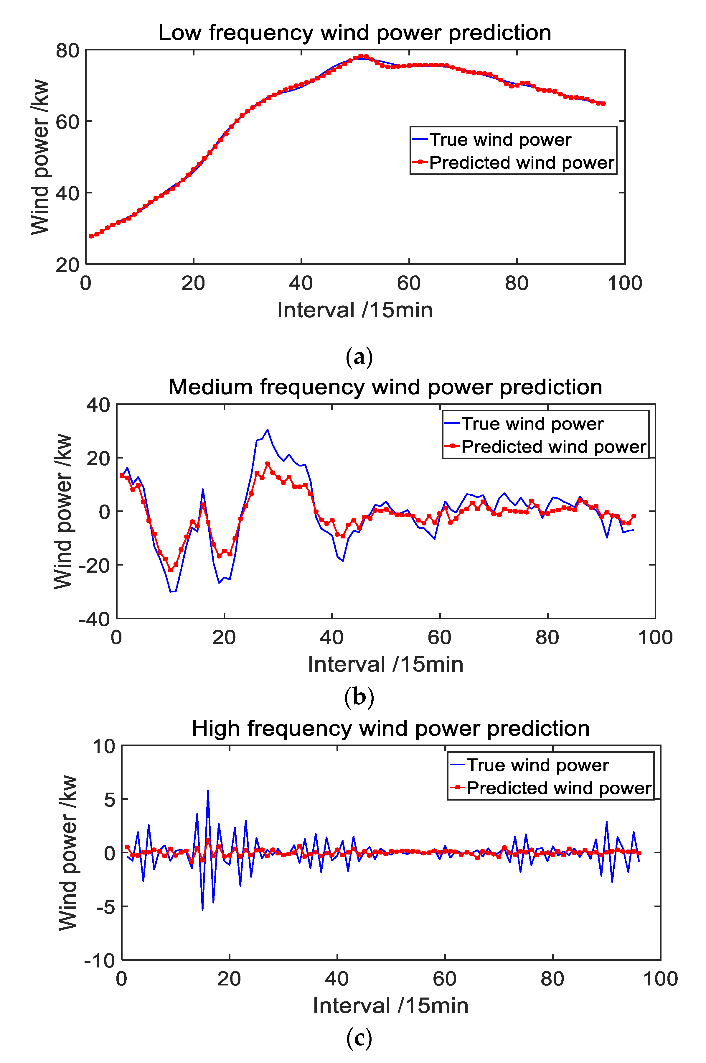
The prediction results of the VMD-improved GWO-ELM model for different frequency decomposition waves are shown in (a), (b), and (c) of Figure 8.

As can be seen from Figure 8, the group of low-frequency waves have the best prediction result with almost no error. The prediction result of the medium frequency wave is worse with small range error. The prediction result of the high-frequency wave is the worst with a wide range of error.

Since the low-frequency wave changes slowly, the prediction model can accurately predict the wind power in the future. By contrast, the high-frequency wave changes faster, which leads to a significant error in the prediction model.

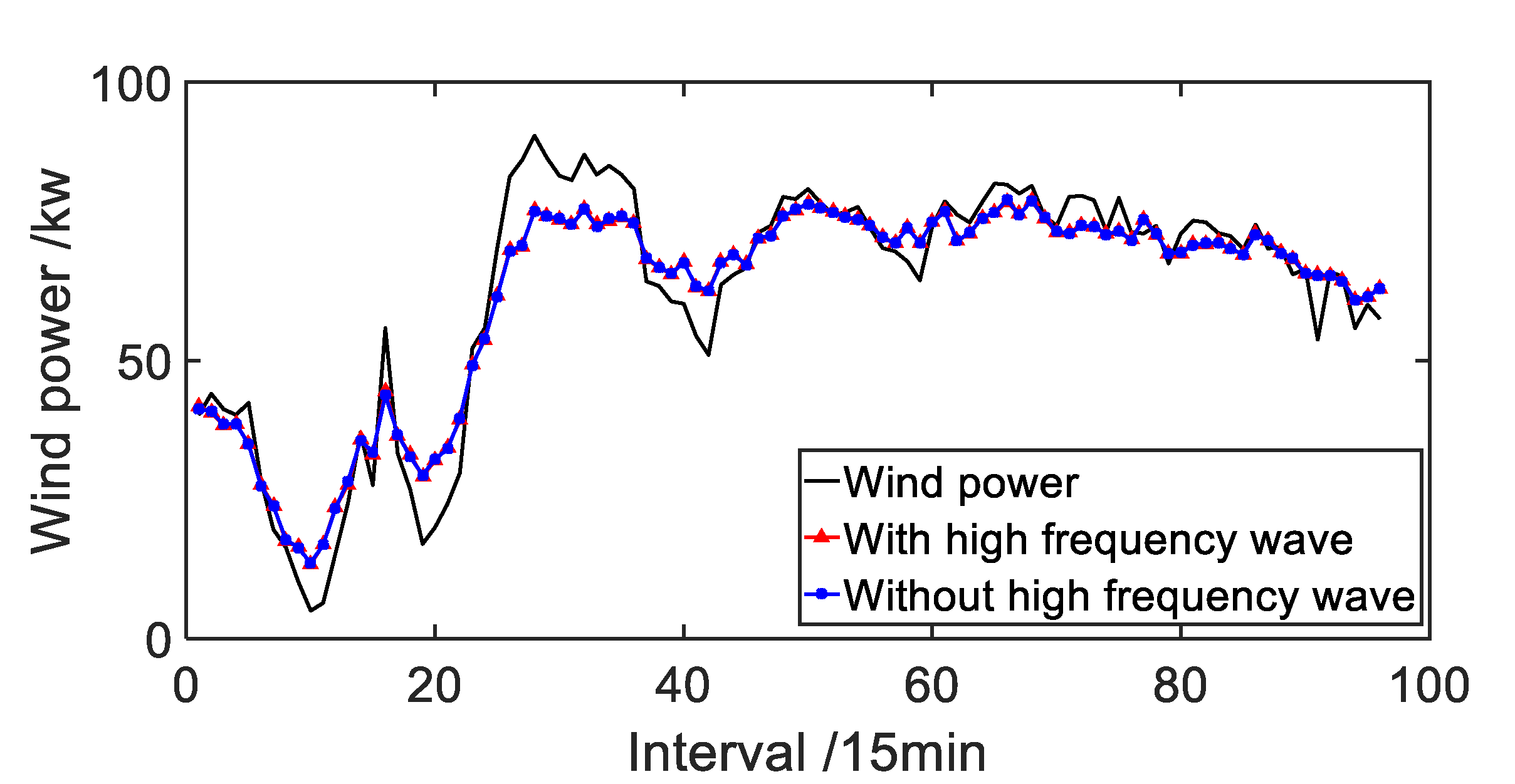
To further indicate the influence of high-frequency waves on prediction accuracy, wind power sequences with or without high-frequency waves were predicted by the VMD-improved GWO-ELM model, respectively. As can be seen from Figure 9, the fitting curve of wind power prediction with or without high-frequency waves is nearly the same.

The predicted evaluation indexes are root-mean-square error (RMSE), mean absolute error (MAE), and mean absolute percentage error (MAPE). The smaller the values of these three indicators, the higher the accuracy of the model. The prediction evaluation indicators are as follows:

$$\begin{gathered} \mathrm{RMSE}=\sqrt{\frac{1}{N}{\displaystyle \sum _{t=1}^N{(y_t-o_t)}^2}} \\ \mathrm{MAPE}=\frac{1}{N}{\displaystyle \sum _{t=1}^N\left|\frac{y_t-o_t}{y_t}\right|\times 100\%} \\ \mathrm{MAE}=\frac{1}{N}{\displaystyle \sum _{t=1}^N\left|y_t-o_t\right|} \end{gathered}$$

(24)

where $N$ is the predicted quantity, $y_t$ is the actual wind power data, and $o_t$ is the predicted wind power data.

In detail, the RMSE, MAE, and MAPE values of waves without high frequency are 5.9433, 4.6467, and 13.09. Correspondingly, these values of waves with high frequency are 5.9113, 4.6219, and 13.01, which are all smaller than the former values. It indicates that the prediction performance of wind power sequence with high-frequency waves is better. On the contrary, the wind power sequence without high-frequency waves will affect the prediction accuracy of wind power.

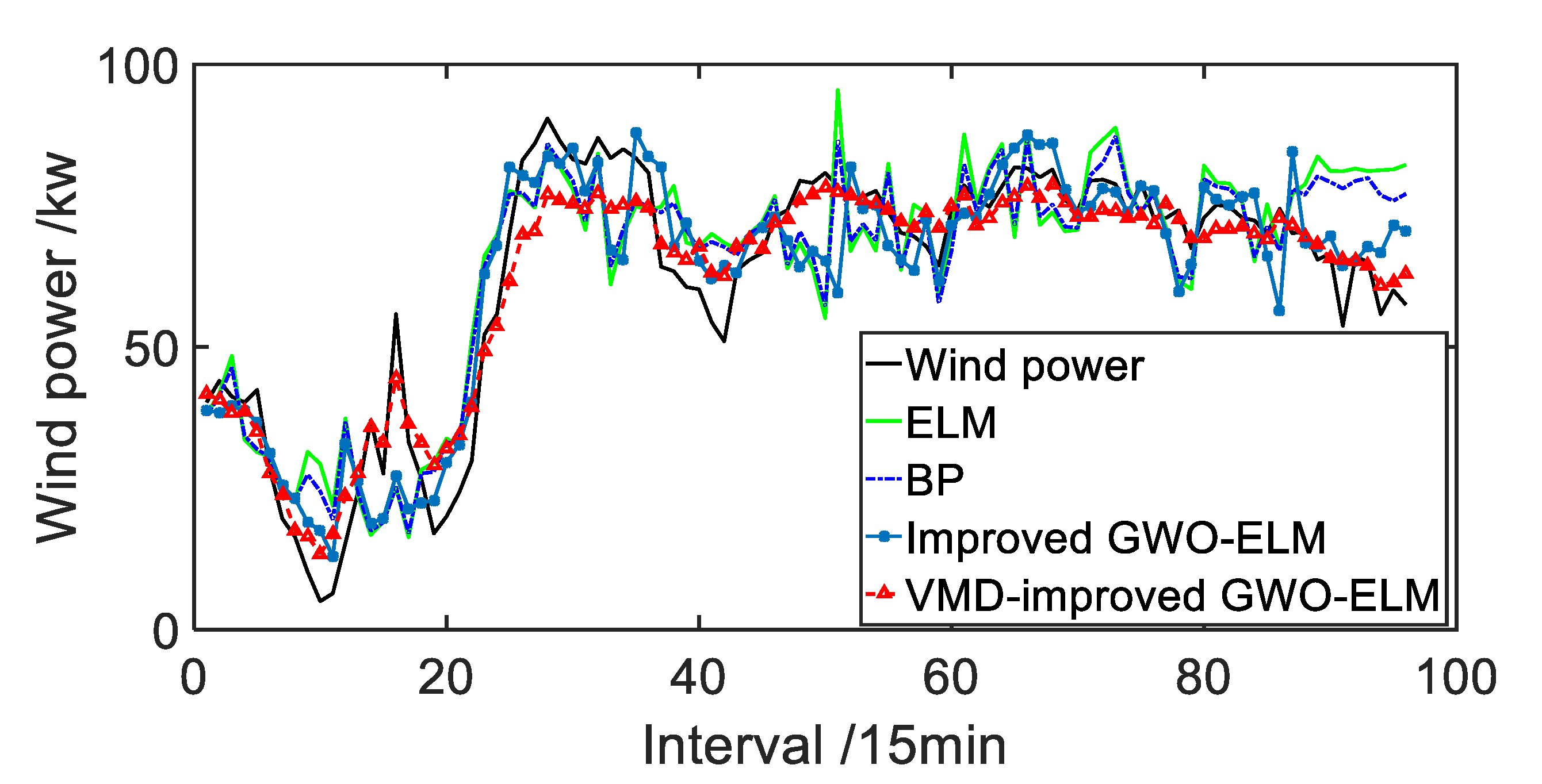
For better analyzing the prediction results, the prediction results of the ELM model, BP neural network model [31], improved GWO-ELM model, and VMD-improved GWO-ELM model were respectively compared.

Set the input node number of the BP neural network [32] model as 5, the number of hidden layer nodes as 8, and the number of output nodes as 1, among which, the number of hidden layer nodes was determined by multiple experiments. The comparison of different prediction results is shown in Figure 10.

As the curves are shown in Figure 10, it is obvious to find that the prediction curve of the VMD-improved GWO-ELM model has the best fitting effect. Correspondingly, the prediction curve of ELM and BP has the worst fitting effect.

In order to further illustrate the effectiveness of the proposed model,

Table 3. Comparison of test results.

Function	Root-Mean-Square Error (RMSE)	Mean Absolute Error (MAE)	Mean Absolute Percentage Error (MAPE)
extreme learning machine (ELM)	12.1494	10.1317	28.14%
back propagation (BP)	10.7536	8.8806	24.57%
Improved GWO-ELM	8.6508	6.6914	17.38%
variational mode decomposition (VMD)-improved GWO-ELM	5.9113	4.6219	13.01%

shows the prediction error indexes of the four models. According to Table 3, the prediction error of the improved GWO-ELM model is smaller than that of the ELM model and the BP model, indicating that the prediction accuracy of the model can be improved by optimizing the parameters of the ELM model with the improved GWO. The prediction error of the VMD-improved GWO-ELM model is smaller than that of the improved GWO-ELM model, indicating that the prediction accuracy can be increased by decomposing the original wind power sequence through the method of VMD before prediction. The VMD-improved GWO-ELM model has the smallest prediction error among the four prediction models, which indicates that the VMD-improved GWO-ELM has a great feasibility in wind power prediction.

5. Conclusions and Prospects

In this paper, a combined forecasting model based on VMD and ELM optimized by the improved GWO algorithm was proposed for short-term prediction of wind power. The following conclusions were drawn through the example simulation:

• The GWO algorithm is improved by changing the linear convergence factor to a nonlinear convergence factor in priority. Then, due to the BAS algorithm’s advantages of paying much more attention to individuals in the searching process, it is combined with the GWO algorithm, which focuses too much on groups, to avoid the algorithm falling into the local optimal solution. Simulation results show that the improved GWO algorithm has high optimization accuracy.
• This paper proposes a method of decomposing the original wind power sequence by using VMD in priority, and then using the improved GWO-ELM model to respectively predict and optimize the decomposing results. According to the simulation results, the decomposed wind power series by VMD can improve the prediction accuracy of the model. The overall prediction model has higher prediction accuracy than the standard ELM model and the BP model.
• However, the predicted time scale for wind power in this paper was only 24 h. For further study, it can be conducted by extending the predicted time scale.
• The prediction accuracy of wind power still needs to be further improved.

References

- Li, J. Research On the Development Prospect of Wind Power Generation in China. China Equip. Eng. 2019, 14, 184–185. [Google Scholar]
- Wang, H.; Han, S.; Liu, Y.; Yan, J.; Li, L. Sequence transfer correction algorithm for numerical weather prediction wind speed and its application in a wind power forecasting system. Appl. Energy 2019, 237, 1–10. [Google Scholar] [CrossRef]
- Li, J.H.; Sang, C.C.; Gan, Y.F.; Pan, Y. Review of Wind Power Prediction Technology Research. Mod. Electr. Power 2017, 34, 1–11. [Google Scholar]
- Cui, Y.; Chen, Z.H.; Liu, L.J. Comparative Analysis of Short-term Wind Power Prediction for Complex Terrain Wind Farms under Abandoned Wind Curtailment. J. Sol. Energy 2017, 38, 3376–3384. [Google Scholar]
- Wang, L.Z.; Liao, X.Z.; Gao, Y.; Gao, S. Review of Modeling and Prediction of Wind Farm Power Generation. Power Syst. Prot. Control 2009, 37, 118–121. [Google Scholar]
- Peng, H.W.; Liu, F.R.; Yang, X.F. Short-term power prediction of wind farm based on artificial neural network. J. Sol. Energy 2011, 32, 1245–1250. [Google Scholar]
- Zhu, K.; Yang, H.M.; Meng, K. Short-term Wind Power Generation Prediction Based on Extreme Learning Machine. J. Electr. Power Sci. Technol. 2019, 34, 106–111. [Google Scholar]
- Sheng, X.C.; Shi, X.; Xiong, W.L. Improved Measurement Method for Extreme Learning Machine Based on Particle Swarm Optimization. Appl. Res. Comput. 2019, 37, 1–6. [Google Scholar]
- Jing, W.T.; Wang, H.R.; Lin, Y.H. Fault Diagnosis of Engine Fuel System Based on IBA-ELM. Comput. Appl. Softw. 2018, 35, 89–93. [Google Scholar]
- Yang, M.; Sun, Y.; Mu, G.; Yan, G.G.; Zhang, M.M. Research on Wind Power Collaborative Prediction Based on Wavelet Real-time Decomposition Mode. J. Sol. Energy 2015, 36, 1639–1644. [Google Scholar]
- Xie, Y.F.; Su, Y.N.; Liu, C.L.; Liu, L.L. Short-term Forecasting of Precipitation Based on Wavelet Decomposition and GA-LSSVM. J. Geod. Geodyn. 2019, 39, 487–491. [Google Scholar]
- Yang, M.; Zhang, Q. Real-time Prediction of Wind Power Based on Set Empirical Mode Decomposition and Correlation Vector Machine. J. Sol. Energy 2016, 37, 1093–1099. [Google Scholar]
- Xue, Y.S.; Chen, N.; Wang, S.M.; Wen, F.S.; Lin, Z.Z. A Review of the Use of Spatial Correlation to Predict Wind Speed. Autom. Electr. Power Syst. 2017, 41, 161–169. [Google Scholar]
- Chen, Y.P.; Mao, Y.; Chen, P.; Tong, W.; Yuan, J.L. Short-term Load Forecasting Based On EEMD—Sample Entropy And ElmanNeural Network. J. Electr. Power Syst. Autom. 2016, 28, 59–64. [Google Scholar]
- Bao, Y.; Dai, B.; Wang, Z.H.; Wang, W.L. Multi-objective Intelligent Home Load Control Algorithm Based on the Grey Wolf Algorithm. J. Syst. Simul. 2019, 31, 1216–1222. [Google Scholar]
- Şenel, F.A.; Gökçe, F.; Yüksel, A.S.; Yiğit, T. A Novel Hybrid PSO—GWO Algorithm for Optimization Problems. Eng. Comput. 2019, 35, 1359–1373. [Google Scholar]
- Guo, Z.Z.; Liu, R.; Gong, C.Q.; Zhao, L. Research on Improvement Based on Grey Wolf Algorithm. Appl. Res. Comput. 2017, 34, 3603–3606+3610. [Google Scholar]
- Lu, G.H.; Teng, H.; Liao, H.X.; Wu, Z.Q. Based on the Improved Power Supply Location and Constant Volume of the Improved Beetle Antennae Search Algorithm. Electr. Meas. Instrum. 2019, 56, 6–12. [Google Scholar]
- Fan, Y.Q.; Shao, J.P. Optimized PID Controller Based on Beetle Antennae.Search Algorithm for Electro-Hydraulic Position Servo Control System. Sensors 2019, 19, 2727. [Google Scholar] [CrossRef] [Green Version]
- Wu, Q.; Shen, X.D.; Sun, G.T. Intelligent Beetle Antennae Search for UAV Sensing and Avoidance of Obstacles. Sensors 2019, 19, 1758. [Google Scholar] [CrossRef] [Green Version]
- Oktay, Y.; Ertan, Y.; Mumtaz, K. A UAV Location and Routing Problem With Spatio-Temporal Synchronization Constraints Solved by Ant Colony Optimization. J. Heuristics 2019, 25, 673–701. [Google Scholar]
- Mellal, M.A.; Zio, E. An Adaptive Particle Swarm Optimization Method for Multi-objective System Reliability Optimization. Proc. Inst. Mech. Eng. Part O J. Risk Reliab. 2019, 233, 990–1001. [Google Scholar] [CrossRef]
- Sankaran, S.K.; Vasudevan, N.; Diderot, K.G.P. Efficient Image De-noising Technique Based on Modified Cuckoo Search Algorithm. J. Med Syst. 2019, 43, 307. [Google Scholar]
- Li, Z.Y.; Mo, J.H.; Shen, Y.L.; Lu, Z.M.; Mao, G.Q.; Yao, S.C. Prediction Model of Pulverized Coal Combustion Characteristics Based on Artificial Neural Network. Boil. Technol. 2019, 50, 49–53. [Google Scholar]
- Huang, G.B.; Zhu, Q.Y.; Siew, C.K. Extreme Learning Machine: A New Learning Scheme of Feedforward Neural Networks. In Proceedings of the 2004 IEEE International Joint Conference on Neural Networks, Budapest, Hungary, 25–29 July 2004; pp. 985–990. [Google Scholar]
- Zhang, W.; Han, W.; Wang, D.; Wang, S.L. Short-term Wind Speed Prediction of the Wind Farm Based on Variational Mode Decomposition and LSSVM. J. Sol. Energy 2018, 39, 194–202. [Google Scholar]
- Jia, Z.D.; Jiang, F.; Wang, H.X.; Li, T.; Yang, J.Y. Grid Load Classification Based on VMD and FCM Clustering Method. Northeast Electr. Power Technol. 2019, 40, 1–6. [Google Scholar]
- Shi, W.G.; Xu, C. Time Delay Prediction based on Phase Space Reconstruction and Robust Extreme Learning Machine. Syst. Eng. Electron. 2019, 41, 417–422. [Google Scholar]
- Han, Y.J.; Li, T.F. Phase Space Reconstruction for Short-term Wind Speed and On-line Prediction of Power Generation. Control. Eng. China 2019, 26, 1503–1508. [Google Scholar]
- Lv, Z.L. Research on Early Fault Diagnosis of Rotating Machinery Based on Variational Modal Decomposition and Optimized Multi-Core Support Vector Machine; Chongqing University: Chongqing, China, 2016. [Google Scholar]
- Zhang, Y.Z. Application of Improved BP Neural Network Based on E-commerce Supply Chain Network Data in the Forecast of Aquatic Product Export Volume. Cogn. Syst. Res. 2018, 57, 228–235. [Google Scholar] [CrossRef]
- Han, S.; Meng, H.; Liu, Y.Q.; Yan, J. Incremental Processing of Wind Power Prediction Model Based on Double Hidden Layer BP Neural Network. Acta Energ. Sin. 2015, 36, 2238–2244. [Google Scholar]
Figure 1.
Convergence factor comparison chart.
Figure 2.
Short-term wind power prediction flow chart based on improved grey wolf optimization (GWO)- extreme learning machine (ELM) model.
Figure 3.
Shubert function convergence curve.
Figure 4.
Four classic test function convergence curves.
Figure 5.
100 KW medium-size wind turbines from a wind farm in Henan.
Figure 6.
The flow chart of improved variational mode decomposition (VMD) decomposition.
Figure 7.
Decomposition of VMD.
Figure 8.
Three frequency waveform prediction sketch diagrams. (a) Low-frequency wind power prediction, (b) medium-frequency wind power prediction, and (c) high-frequency wind power prediction.
Figure 9.
With/without high-frequency wave wind power prediction.
Figure 10.
The comparison of different prediction results curve.