Coupling Layout Optimization of Key Plant and Industrial Area

1
School of Chemical Engineering and Environment, China University of Petroleum (Beijing), No. 18 Fuxue Road, Changping, Beijing 102249, China
2
School of Chemical Engineering and Technology, Xi’an Jiaotong University, No. 28 Xianning West Road, Xi’an 710049, China
*
Author to whom correspondence should be addressed.
Processes 2020, 8(2), 185; https://0-doi-org.brum.beds.ac.uk/10.3390/pr8020185
Submission received: 10 December 2019
/
Revised: 29 January 2020
/
Accepted: 3 February 2020
/
Published: 5 February 2020
(This article belongs to the Special Issue Process Optimization and Control)
Abstract
:Layout problems are an engineering task that heavily relies on project experience. During the design of a plant, various factors need to be considered. Most previous efforts on industrial layout design have focused on the arrangement of facilities in a plant. However, the area-wide layout was not thoroughly studied and the relationship between plant layout and area-wide layout was rarely mentioned. In this work, the key plant that has the greatest impact on the industrial area is figured out first, and then the coupling relationships between the key plant and the industrial area are studied by changing the occupied area and length-width ratio of the key plant. Both of them are achieved by changing the floor number. A hybrid algorithm involving the genetic algorithm (GA) and surplus rectangle fill algorithm (SRFA) is applied. Various constraints are considered to make the layout more reasonable and practical. In the case study, a refinery with 20 plants is studied and the catalytic cracking plant is found to be the key plant. After the retrofit, the total cost of the refinery is 1,806,100 CNY/a less than that before, which illustrates the effectiveness of the method.
1. Introduction
Facility layout problem (FLP) is an important branch of industrial engineering and has a great impact on production efficiency, operating safety and construction investment of a factory. It was firstly proposed by Koopmans and Beckmann [1] in 1957, aiming to minimize the material handling cost by arranging given facilities reasonably. The research direction of early layout problems was the single-floor layout of equal-area facilities using a discrete QAP (Quadratic Assignment Problem) model [2]. The area was divided into grids of the same size in one-to-one correspondence with the facilities. Since the facility shape [3,4] and size have an obvious impact on the overall layout area, it is unreasonable to generalize the layout problem with equal size facilities. Therefore, some works tended to convert the direction into UA-FLPs (Unequal-Area Facility Layout Problems) [5]. Due to the shortage of land resources and limited horizontal space, a multi-floor layout has become one of the research hotspots [6]. Various methods to assign facilities into floors have been implemented. Chang et al. [7] classified the departments into groups according to the flow relationship, and the departments of a similar category are arranged on the same floor. Wang et al. [8] divided facilities into different floors by stochastic algorithm, and obtained an optimal solution iteratively.
Many efforts have been made to rationalize the layout results. Safety factors were implemented by the TNT (Trinitrotoluene) explosion model [9] or domino hazard index [10]. Limitations on the area and aspect ratio of facilities were taken into account as well [11,12,13]. The adjacent arrangement of special plants was implemented by arranging plants with upstream and downstream relationships jointly [14]. The same objective was also achieved by maximizing the adjacent lengths of plants with frequent flow exchanges [15,16], or the total flow rate of departments next to each other [17]. In order to make the mathematical models more accurate, a number of works have been done. Ahmadi and Jokar [18] established a multiple-stage model in multi-floor layout research. Facilities were assigned to each floor using mixed integer programming (MIP), and the facility location on the floor and the final layout were determined by non-linear programming (NLP). Anjos and Vieira [19] firstly optimized the relative location of departments in the region and then determined the inner precise layout. The model solved sequentially may lead to suboptimal solutions, so Leno et al. [20] proposed a hybrid algorithm to optimize the internal and external layout at the same time. Various algorithms were adopted, such as GA [21,22] and the simulated annealing algorithm [23,24], and both of these have obtained reasonable results. To improve the performance of each algorithm, many kinds of hybrid algorithms [25,26] were often applied as well.
However, through the development of layout research in recent years, there are still some aspects left to be solved or improved. In order to solve such problems, some concepts need to be clarified. There are two main types of layout—namely, plant layout and area-wide layout (general layout) [27]. A plant is defined as a collection of multiple facilities, and the industrial area usually contains various plants. Plant layout is mainly devoted to the optimal arrangement of facilities with their original sizes in the plant area. Area-wide layout studies focus on the reasonable placement of plants with fixed or flexible sizes within the industrial area. The main purpose of both layouts is to reach the reasonable use of space and meet process requirements. However, the studied land scale of the area-wide layout is much larger than the plant layout, which results in more complicated factors that need to be considered, such as geographical factors and traffic conditions. Additionally, pipeline network design plays a more important role in the area-wide layout because of the long distance, which brings more solving difficulties as well. Therefore, at present, more attention is paid to the study of plant layout [28,29,30,31], and unfortunately, only a small number of researchers have focused on the area-wide layout [32,33] due to its complexity. The coupling optimization of both is even rarer. However, it is quite essential because these two layouts are indivisible. Plant layout usually has an effect on the area-wide layout to some extent, especially in the aspect of the occupied area. If it is required to reach the best of both, plant layout must be considered in the design of the area-wide layout. To the best knowledge of the authors, few previous articles consider the impact of a single plant on the overall area, or whether a better scheme can be obtained if both layouts are taken into account at the same time. In addition, in previous studies, the number of facilities or plants was generally small due to the solving difficulty of layout problems. The number of facilities considered in the optimization was less than 10 in most of works [34,35]. Even in some works with a larger problem size, there were around 20 facilities in total [36], which is still far from the actual situation.
Therefore, to deal with the above issues, a new idea to design an area-wide layout is put forward. The main contribution of this work lies in the development of the conventional single-layout studies, which means that the coupling optimization of the two layouts mentioned above is realized by several steps of optimization. The impact of plant layout on the area-wide layout is emphasized. This work focuses on improving the practicality of the layout optimization method and explores the internal relationships of different levels of layouts. The plant layout and area-wide layout are concerned at the same time and the coupling relationships between them are especially considered. The main purpose of this work is to figure out the impact of a special plant on the overall industrial area and the coupling relationships between a plant and the industrial area, so that some new construction ideas can be provided. This area has significant research value but has rarely been mentioned in previous studies. It is very beneficial if the cost of the industrial area can be greatly reduced by only modifying one certain plant. To achieve the above objectives, a method with multiple steps is proposed to solve the problem sequentially. Firstly, the key plant with the greatest impact on the overall layout is figured out and modified. It is then coupled with the industrial area. The whole layout with all the plants is optimized and compared with the original one to study the impact of changes in the key plant on the overall layout. Through the above steps, plant layout is well related to the area-wide layout. In addition, based on previous research, safety distance, multi-floor model and joint arrangement of special facilities are applied. A case with practical size is studied. A combined algorithm of the genetic algorithm (GA) and surplus rectangle fill algorithm (SRFA) is adopted to give rules for facility placement and optimize layout results effectively. As a conclusion, the point of this work is that a common problem which has not been studied before is raised and a set of approaches to address it is put forward. Through the case study, a better solution than the original one is certainly obtained due to the more comprehensive approach.
2. Problem Statement and Mathematical Model
Layout problems are known to be complex and NP-hard [37] with plenty of variables and constraints. On the premise of given facility sizes and flow information, the optimal relative location of facilities with minimum cost are the ultimate goal for the final layout. Since there are two levels of layouts in this study, both facility arrangement and plant placement are considered. To solve this problem, some assumptions and rules are given as follows:
- ➢
- Both plants and facilities are simplified as rectangles and placed orthogonally;
- ➢
- Plants cannot overlap each other, as with facilities;
- ➢
- Safety distance between facilities should meet the requirements in the regulations;
- ➢
- Multi-floor structure is applied. Facilities can be placed on the first floor or higher.
Based on the descriptions above, a mathematical model was established for the layout problem with constraints and the objective function.
2.1. Constraints
In addition to the basic settings, a set of constraints is necessary for a more practical layout result to ensure the rationality of the facility and plant arrangement. These constraints include several aspects. Directional constraints, non-overlapping constraints and boundary constraints can be used in both plant layout and area-wide layout. Cross-floor constraints, pump area constraints, parallel heat exchanger constraints and facility floor constraints are applied only to plant layout [14]. They are explained, respectively, in detail below.
Directional constraints limit the orientation of facilities (or plants) that can be placed horizontally or vertically within the given area. The visual length and width of facilities in the region are determined by the direction. A binary variable ri is set and specify that if ri = 0, the facility is placed horizontally, otherwise, if ri = 1, the facility is placed vertically. The relationship between the visual length and width of a facility in the region and its actual size can be described as follows:
where li and wi are the visual length and width after facility placement and lai and wai are the actual size of the facility. These constraints are also applicative for plant placement. They are also set as linking constraints between plant layout and area-wide layout. The length, width and aspect ratio of the key plant (explained in the next section) are determined through the results of the plant optimization and are regarded as known conditions in subsequent optimization. The sizes of other plants remain as original ones according to the case.
Non-overlapping and boundary constraints guarantee the rationality of the final layout, and are suitable for both facilities and plants. Different facilities (or plants) cannot be placed in the same position, and the area occupied by different facilities cannot be crossed. This can be achieved by non-overlapping constraints. When the relative positions of facility i and j meet one of the following four conditions, they are non-overlapping:
where i and j represent two different facilities. For facility i, x1i and y1i are the coordinates of the lower left corner, and x2i and y2i are the coordinates of the upper right corner. Formulas (3)–(6) respectively represent that facility i is on the left, right, upper and lower side of facility j.
In addition to the fact that facilities (or plants) cannot overlap with each other, they cannot be placed beyond the given area, which is achieved by boundary constraints. Only when the position of a facility meets all the following constraints can it be arranged without exceeding the given region:
where L and W are the length and width of the given area. For facilities, the area means a plant, and for plants, it means the industrial area. When all the facilities are placed, the overall area occupied is the obtained plant area. It is noted again that the above kinds of constraint are suitable for both facility and plant arrangement, and the following ones are only used in plant layout to arrange facilities.
Cross-floor constraints for high facilities are necessary for multi-floor studies. When it comes to three-dimension problems, floors should be taken into account. The floor height is usually predetermined, and high facilities like towers and reactors would occupy multiple floors when they are arranged. When the position K on the first floor is occupied by a high facility, the same position on the higher floor cannot arrange other facilities. K is set as a binary variable to realize the function. For a high facility i, Ki = 1 means facility i is placed at position K. Take a two-floor plant as an example, the constraint can be explained as follows:
where K1i is the position of facility i on the first floor, and K2i is same position on the second floor; i is a high facility that needs to be placed across floors; and K2j is the position of facility j on the second floor. Equation (11) indicates that if the cross-floor facility is placed at position K, the other facilities cannot be arranged at position K on any floor.
The pump area constraints seek to ensure that the pumps should be arranged as a whole to facilitate operation and maintenance, referring to the actual situation of the industry. The area occupied is called pump area. In the pump area, the orientation of the pumps is set to be fixed for the layout regularity. With the relative position of pumps and the coordinates of the pump area, the actual position of each pump in the plant area can be described as follows:
where xpi and ypi are the actual coordinates of pump i. xp and yp are the coordinates of the pump area. xpri and ypri are the coordinates of relative position of pump i inside the pump area.
Parallel heat exchanger constraints aim to reach a joint arrangement of heat exchangers with the same function. In the actual situation, in order to meet the requirements of heat transfer, parallel heat exchangers should be placed together as a whole in the layout. Different from the pump position that needs to be optimized, the relative position of the heat exchangers in parallel are often fixed. In order to arrange the heat exchangers neatly, they are set to be placed horizontally. When there are, in total, n heat exchangers in a parallel group, the coordinates of each heat exchanger inside can be calculated as:
where i is the number of a heat exchanger that belongs to a parallel group. xHi and yHi are the actual coordinates of heat exchanger i in the overall plant. xH and yH are the coordinates of the group, and wHi is the width of heat exchanger i.
Facility floor constraints mean that facilities with special features should be positioned on a certain floor so that their function is ensured. Pump area should be placed on the first floor to avoid cavitation. Air coolers need to be placed on the top floor to ensure their cooling effect. High facilities like towers and reactors must be placed on the first floor because of their height, and need to occupy the same position on each floor.
2.2. Objective Function
To solve plant layout problems, when all the constraints are satisfied, the objective function of the total cost (TC) including piping investment cost (PIC), pumping operating cost (POC), land cost (LC) and floor cost (FC) is established, and all the costs are expressed in the form of annual costs:
PIC is related to the pipeline material cost and installation cost, and is calculated by the pipeline length and unit price:
where T is the plant life; m is the serial number of a material connection between different facilities; n is the number of total material connections; Lm is the Manhattan distance between the center coordinates of the two rectangular facilities, in the unit of m; and UICm is the unit price of pipeline (USD/m), which is calculated by the method proposed by Stijepovic and Linke [38]:
where xi and yi are the coordinates of the center point of facility i, and xj and yj belong to facility j; A1 is the pipe cost per unit of quality, which is 0.82 USD/kg; wtpipe is the quality per meter of pipe, in the unit of kg/m; A2 is the installation cost parameter, which is 185 USD/m0.48; Dout is the outer pipe diameter in the unit of m; A3 is the floor space cost of pipe, which is 6.8 USD/m; and A4 is the insulation layer cost of pipe, which is 295 USD/m. The values of wtpipe, Dout and related parameters are determined by Equations (20)–(22) [38]:
where Dinner is the inner diameter of pipe in the unit of m; Q is the material mass flow rate in the unit of kg/s; ρ is the material density in the unit of kg/m3; and u is the flow rate in the unit of m/s.
The annual pumping operating cost POC means the material handling cost, and it is determined by Equation (23):
where, CE is the unit energy cost (USD/kW·h), H is the annual operating time (h/a), and Pm is the pump work of transporting different materials (W), which is calculated by Equation (24):
where η is the pump efficiency; hf,m is the energy consumed by overcoming the resistance along the way and gravity in the process of unit material transmission in the unit of J/kg, which is determined as:
where λ is the coefficient of friction; g is the gravity constant; z is the transmission height in the vertical direction (m); and αm is a binary variable which represents the material transportation in the vertical direction. If a material flow is transferred from a lower floor to a higher floor, the material handling cost includes the upward transfer cost, then αm = 1. Otherwise, αm = 0.
The calculation of land cost (LC) and floor cost (FC) is related to the area occupied by all the facilities, as shown in Equations (26) and (27).
where UL is the unit land cost and UF is the unit floor cost (CNY/m2). x1i and y1i are the lower-left coordinates of facility i. li and wi are the length and width.
In total, TC is set for the optimization of plant layout with four kinds of costs. However, there is a difference between the optimization of the industrial park and plants. This work focuses on exploring the impact of changes in plant area on the area optimization of the industrial park. Therefore, in the optimization of the area-wide layout, only the land cost is chosen to be the objective function for optimization. The method to calculate LC in area-wide layout is the same as the one in Equation (26) and x1i, y1i, li, wi are parameters of the related plants.
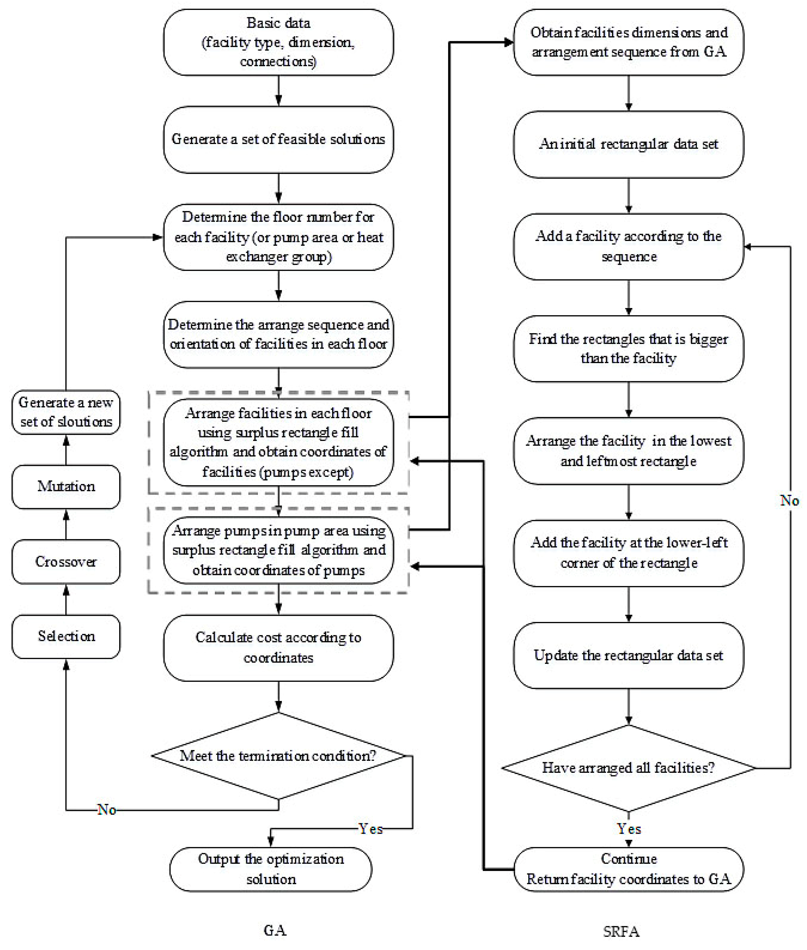
3. Optimization Algorithm
For the layout problems, the facility position, order, material connections, occupied area and investment costs are the issues that need to be addressed. In this work, in order to reach a final layout, a hybrid algorithm combining GA and SRFA is proposed to solve the problem.
GA [39] is applied as the main framework of the whole algorithm. GA searches for the global optimal solution by simulating the biological evolution process in nature. In GA, each population is composed of multiple individuals, and chromosomes are made up of multiple genes, which determine the fitness of individuals. Iterative operation is carried out through selection, crossover and mutation. Individuals with high fitness are passed on until the optimal result is obtained.
As a classical evolutionary algorithm, GA has strong flexibility and global search ability, and the genes can be mapped to the research facilities one by one. Therefore, it is one of the most widely used algorithms in the facility layout field [40]. In this work, multiple facilities are coded by genes to obtain the desired optimal plant layout. In the model, variables are set to be genes, and their value ranges are chosen to be 0.5–10.49. Each gene represents a decision variable, including the facility placement order, the orientation and the bottom width of the given region. The objective function is regarded as fitness. By randomly generating variable values and iterating optimization, the result output with the highest fitness is finally obtained, which is the optimal layout result under GA.
However, although GA has a good performance, it is difficult to consider the size and area of facilities in the programming process, so an additional algorithm is needed to arrange the rectangular facilities into the rectangular region in a tight and orderly manner. SRFA is a suitable algorithm that has the above functions [8]. It is initially used to cut a rectangular plate into rectangular blocks of specific sizes to reach the highest utilization of the original plate. Therefore, for the layout problem with rectangles of both facilities and plants, it is significantly suitable and effective in performance, aiming to minimize the area occupied by facilities within a given area [41].
SRFA is expressed in a data set of residual rectangles to represent all the available space currently. All the facilities are arranged into the region in a given order. When a new facility is put into the plant, an appropriate area is figured out in the residual rectangle set. Facilities are placed in the lower left corner preferentially in the residual area, and the coordinates and sizes are recorded in an array. After a facility is arranged, the number set of residual rectangles is updated for the next placement. The residual rectangles with no area occupied or that are no longer able to be disposed of by any of the remaining facilities will be removed. All the facilities are arranged in this manner until all of them are arranged completely, and all the facility positions are obtained.
SRFA can reach the facility coordinates of each floor, but it requires the placement order and the bottom edge length of the region to do the calculation, so this is combined with GA to get a final layout result. The placement order, direction of each facility and the plant bottom length are variables that have a significant impact on the modeling and calculating process, and they are decision variables that should be given before calculation for SRFA. Therefore, these variables are generated in GA and then sent to SRFA to obtain the facility coordinates. Values obtained from the SRFA are returned back to GA to calculate the fitness. Through the process of selection, crossover and mutation, the results of each generation are iterated until the preset number of iterations is reached or the optimal solution is obtained. If it is set to be a multi-floor structure, the floor number should be predetermined, and the number of facilities in each floor are generated in GA within a given range. Due to the large number of facilities inside the plant and the excessive number of variables set in GA, the running time of the combined algorithm is relatively long. Therefore, parallel computing is adopted to improve the running speed and save calculation time. When the plant is set to be a two-floor structure, then the specific optimization steps of a plant layout with multiple facilities are as follows:
- ➢
- A series of random variables are generated in GA as the initial population, which determine the facility placement order and direction, the facility number in each floor and the length of the bottom edge of the plant area.
- ➢
- Since pumps, towers and reactors must be placed on the first floor and air coolers must be placed on the top floor, these special facilities are put aside. Other facilities are randomly sorted according to the variable values generated by GA, and the order is recorded in an array called P.
- ➢
- The value of the variable a determines the number of facilities placed on the first floor. In order P, the first a facilities are placed on the first floor, and the other facilities are placed on the second floor.
- ➢
- Add pump area, towers and reactors to the facilities of the first floor, and a new sort P1 of the facilities on the first floor is randomly generated. The layout of the first floor is optimized by SRFA, and the facility position coordinates are obtained and recorded in array A1. Since towers and reactors need to be placed across the floors, array B is used to record their locations.
- ➢
- Add air coolers to the facilities on the second floor, and a new sort P2 is generated randomly. Facilities on the second floor are also optimized by SRFA. Before the optimization, the positions recorded in array B are deleted from the available area on the second floor to ensure that the towers and reactors can be placed across the floors and do not overlap with other facilities on the second floor. The position coordinates of the facilities on the second floor are recorded in array A2.
- ➢
- The layout of the pump area on the first floor is optimized by SRFA, as well according to the order of pump placement. The coordinates of each pump are determined and added to array A1.
- ➢
- Calculate the total cost including pipe construction cost, material handling cost, land cost and floor cost, and obtain individual fitness values according to the position coordinates and sizes of each facility and material connection data in GA.
- ➢
- The current population in GA is judged. If it has reached the preset evolution number, the program will stop running; otherwise, a new generation of random variables will be generated through selection, crossover and mutation, and then step 2 will be carried out again to continue the operation.
It should be noted that the hybrid algorithm was carried out in MATLAB. The built-in GA in MATLAB toolbox was used, and all kinds of operators were default during the optimization process. In detail, the selection function is stochastic uniform, and the mutation function and crossover function are both constraint dependent. In order to introduce the combination of the two algorithms more intuitively, the algorithm flow diagram of the proposed methodology is shown in Figure 1.
4. Optimization Process
This section shows the main contribution of this work. As mentioned in the introduction, plant layout has an obvious impact on the area-wide layout. Therefore, the research of only a single layout is not comprehensive, and considering two levels of layouts in one work will certainly lead to a better overall solution and provide a new idea for the industrial retrofit. Thus, in this work, it is necessary to realize the coupling optimization between the internal layout of a plant and the general layout for the industrial area. To study the coupling relationships between two layouts, the transformation of a certain plant needs to be carried out, and then the modified plant together with other plants is optimized in the industrial area. The results before and after the transformation are compared. In order to achieve the above goals, the overall optimization process is divided into several parts and the results are obtained step by step.
In the first part, the key plant is figured out. It is defined as the plant with the greatest impact on the overall occupied area. When the area or sizes of the key plant changes, the reduce in the total industrial area is the largest. To seek out the key plant, it is necessary to obtain the impact of each plant on the area-wide layout, and the plant with the greatest effect is taken as the optimization target. A variable e is specially defined in this work as the ratio of industrial area variation to plant area variation. When the plant area decreases, the larger value of e means that the reduction of the target plant area can reduce the overall industrial area more effectively. By comparing e of each plant, the key plant is easy to be figured out.
In the second part, the layout of the key plant is optimized using the proposed hybrid algorithm. The changes of occupied area and aspect ratio of the key plant are achieved by optimizing the internal layout and increasing the number of floors. The total cost including pipe construction cost, material handling cost, land cost and floor cost is taken as the objective function.
In the third part, the coupling relationships of the key plant and industrial area are studied. The original and modified layouts of the key plant are respectively optimized with the remaining plants in the objective function of minimizing the land cost. The overall industrial layout before and after the modification of the key plant is analyzed and discussed.
In total, the proposed method can deal with the coupling layout problems through several steps. A set of process approaches are put forward. Previous research has only focused on a single layout and ignored the coupling relationships of different levels of layouts, which may lead to an incomprehensive result. When both of the two layouts are concerned in one work, a better coupled result of the overall layout will be certainly obtained. This idea can be proved in the case study.
5. Case Study and Result Discussion
In order to prove the effectiveness of the optimization process and the proposed methodology, a refinery was taken as an example. There were 20 plants in total, e.g., a power station (PS), crude oil fractionation plant (COF), gas separation (GS), hydrogenation union (HU), residual and wax oil hydrodesulfurization (RWH), fluidized catalytic cracking (FCC), light hydrocarbon recovery (LHR), LPG desulfurization and demercaptan (LPGDD), sulfur recovery (SR), aromatics combine plant (AC), hydrogen production (HP), continuous catalytic reforming (CR), naphtha hydrofining (NH), polypropylene and polyester (PP), delayed coking (DC), air separation and compressor (ASC), central control room (CCR), railway transportation department (RTD), tank field (TF), and sewage treatment area (STA). The initial sizes of the plants are shown in Table 1. It should be noted that the lengths and widths include both the original plant sizes and the safety distances.
5.1. Process of Finding the Key Plant
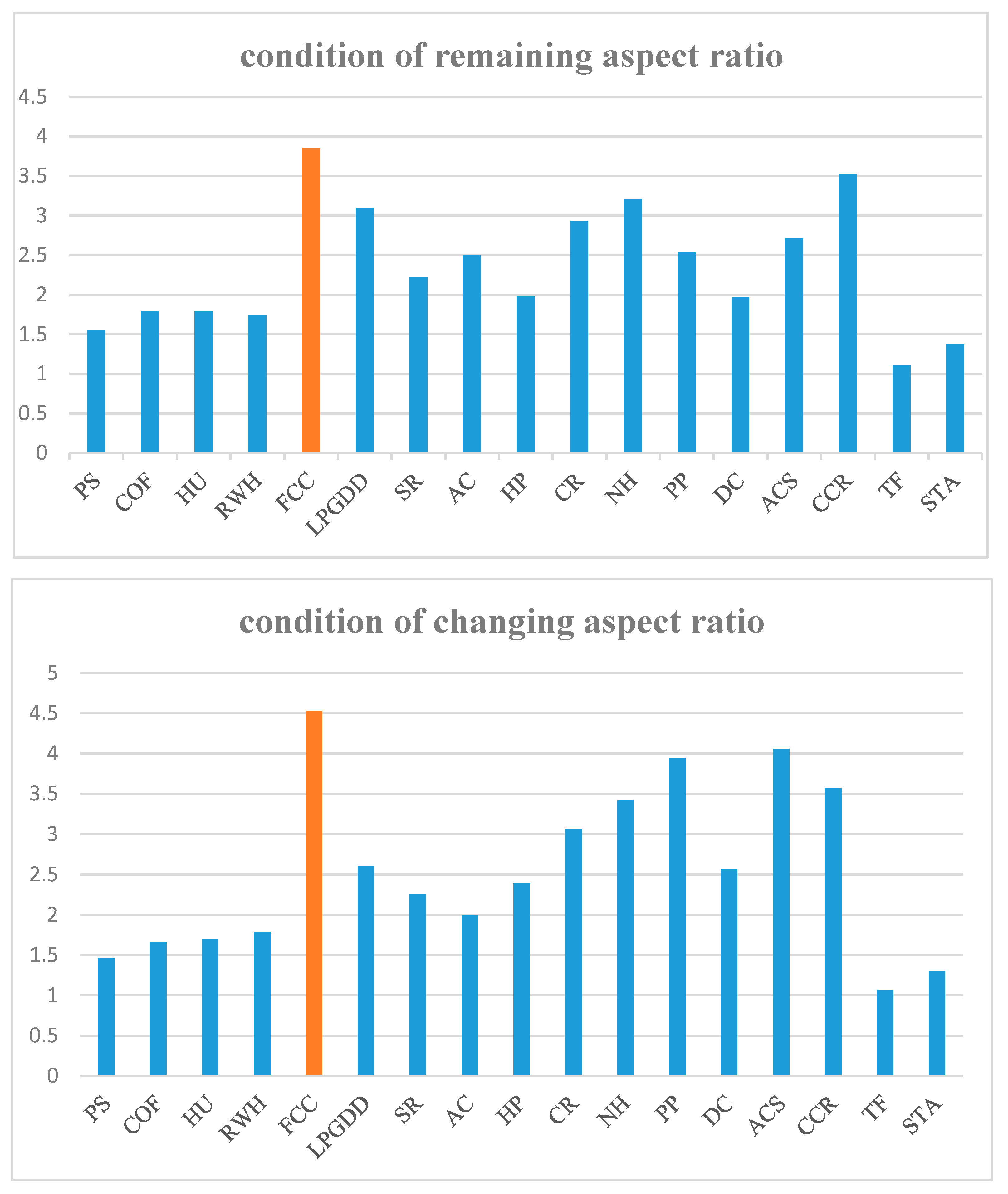
In this section, the key plant with the greatest impact was found based on our methodology. Because the changes of the area and aspect ratio theoretically affect the overall industrial area, the two aspects were both studied. The area and aspect ratio of each plant were adjusted one by one while the sizes of other plants remained unchanged. The aim of this action is to study the influence on the area-wide layout of each plant. Two scenarios were used for the study. One scenario only changed the area of a certain plant, and the other adjusted the area and aspect ratio simultaneously.
When studying the area change of a plant, it was assumed that the area of the modified plant is 20%, 40%, 60% and 80% of the original one. The minimum of the occupied industrial area was set to be the optimization objective, and the e value of each plant was calculated one by one. When the area and aspect ratio were simultaneously changed, the area was still calculated as above, and the aspect ratio was regarded as a random variable with a certain upper and lower bound according to the inner structure of the plant. The aspect ratio was calculated with other variables in GA to obtain the modified plant layout and calculate the e value of the plant. The values of e of each plant with different areas and aspect ratios are listed in Table 2. Since GS and LHR are too small compared with other plants and have little impact on the overall layout, they are excluded from the selection of the key plant. RTD is not eligible to be the key plant because its size is fixed.
In order to display the results more intuitively, the average value of e under the two different conditions was calculated and is drawn in Figure 2.
As mentioned above, the larger the value of e, the greater the influence of the plant on the area-wide layout. Combined with Table 2 and Figure 2, it can be seen that when only the area of a plant changes, the average e value of the FCC plant is higher than other plants. When both the aspect ratio and area are changed, the e value of the FCC plant is still larger in each area condition and is the largest in average. In particular, when the area is 80% of the original one, e reaches 7.07. This shows that the FCC plant has a much greater impact on the area-wide layout than other plants. When the area of the FCC plant is modified, the overall area can be significantly reduced. Therefore, the FCC plant was selected as the key plant in this case.
5.2. Internal Layout Optimization of the Key Plant
Through the efforts above, FCC was selected to be the key plant with 217 facilities in total, including 48 heat exchangers, 70 vessels, five reactors, six towers and 79 pumps, and 224 material connections. Since it was proved to be an effective way of modifying the key plant, the changes in the area and aspect ratio of the FCC plant were carried out at the same time by building a double-floor structure and modifying the inner layout of each floor.
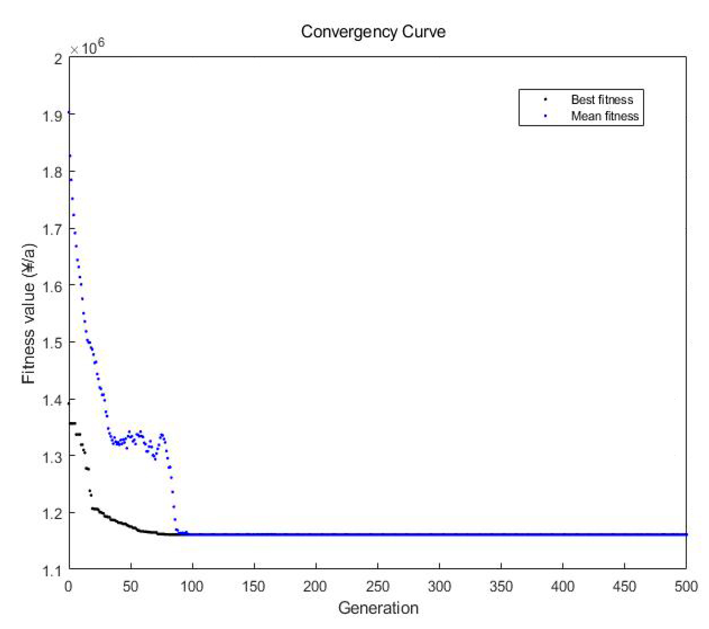
For the internal layout of the FCC plant, the bottom length of the plant was set as a variable with 20 m lower bound and 60 m upper bound. The floor height was set as 6 m. Pumps were centrally arranged in a pump area with 16 rows and five columns on the first floor. Air coolers were placed on the second floor. Towers and reactors were placed across floors. Their shapes in a two-dimensional plane were circles and were treated as rectangles with sides equal to their diameters for the convenience of arrangement. Parallel heat exchangers were placed as groups with other facilities. The algorithm combining GA and SRFA was applied to solve the mathematical model by using parallel computation on MATLAB with the objective of minimizing the total cost. Figure 3 shows the plant layout plan after the modification, and Table 3 shows the comparison of the sizes and costs of the original and modified plant layout. Figure 4 shows the convergence curve of the hybrid algorithm. Due to the adoption of parallel computing, the calculation speed was greatly increased, and the computing time for the optimization of the layout inside the FCC plant was around 300 s.
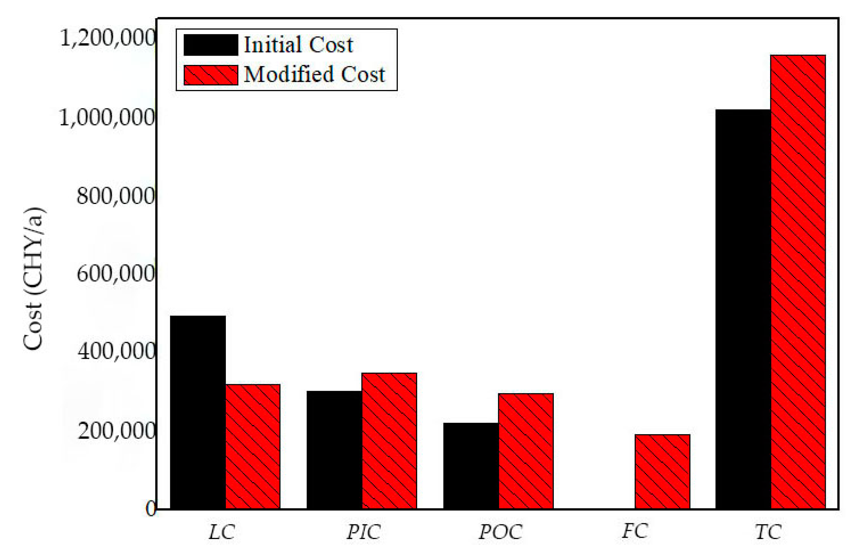
It can be seen from Table 3 that, after the modification, the area of the FCC plant is 64.89% of the original one. However, in terms of costs, the original layout is superior. After the modification, the total cost is higher. In order to facilitate comparative analysis, the comparison of five kinds of cost of the key plant is drawn in Figure 5.
Combined with Figure 3 and Figure 5 and Table 3, it can be seen that the modified layout satisfies the constraints established in the model; however, its total cost is higher than the original layout, which is 1.1625 million yuan per year.
As for LC, the land cost of the double-floor modified layout is lower, which is 64.89% of that of the original single-floor layout. However, in the ideal case where all the facilities can be arranged without constraints, the land cost should be 50% of the original one when an additional floor is added. The reason is that, firstly, the practical constraints must be satisfied. Secondly, towers and reactors occupy the same position on the two floors at the same time. Additionally, pumps must be placed on the first floor as a pump area, which limits the area of the first floor and may lead to the loose layout of other floors. Therefore, the land cost is 64.89% of the original one, instead of 50%. The pipe investment cost PIC and pumping operating cost POC after the modification are both higher. This is because the materials are transformed horizontally in the single-floor layout and only needs to overcome friction resistance. When it becomes a multi-floor structure, cross-floor connections are added, and the more connections in the vertical direction there are, the longer the vertical conveying distance will be. In addition to overcoming the friction resistance, the materials need to overcome gravity, which increases the energy consumption and leads to the increase in the operational cost. After the modification, due to the addition of floors, the floor construction cost FC needs to be taken into account. As for the total cost, after the modification, it is 141,400 CNY/a higher than the original cost.
5.3. Coupling of the Key Plant and Industrial Area
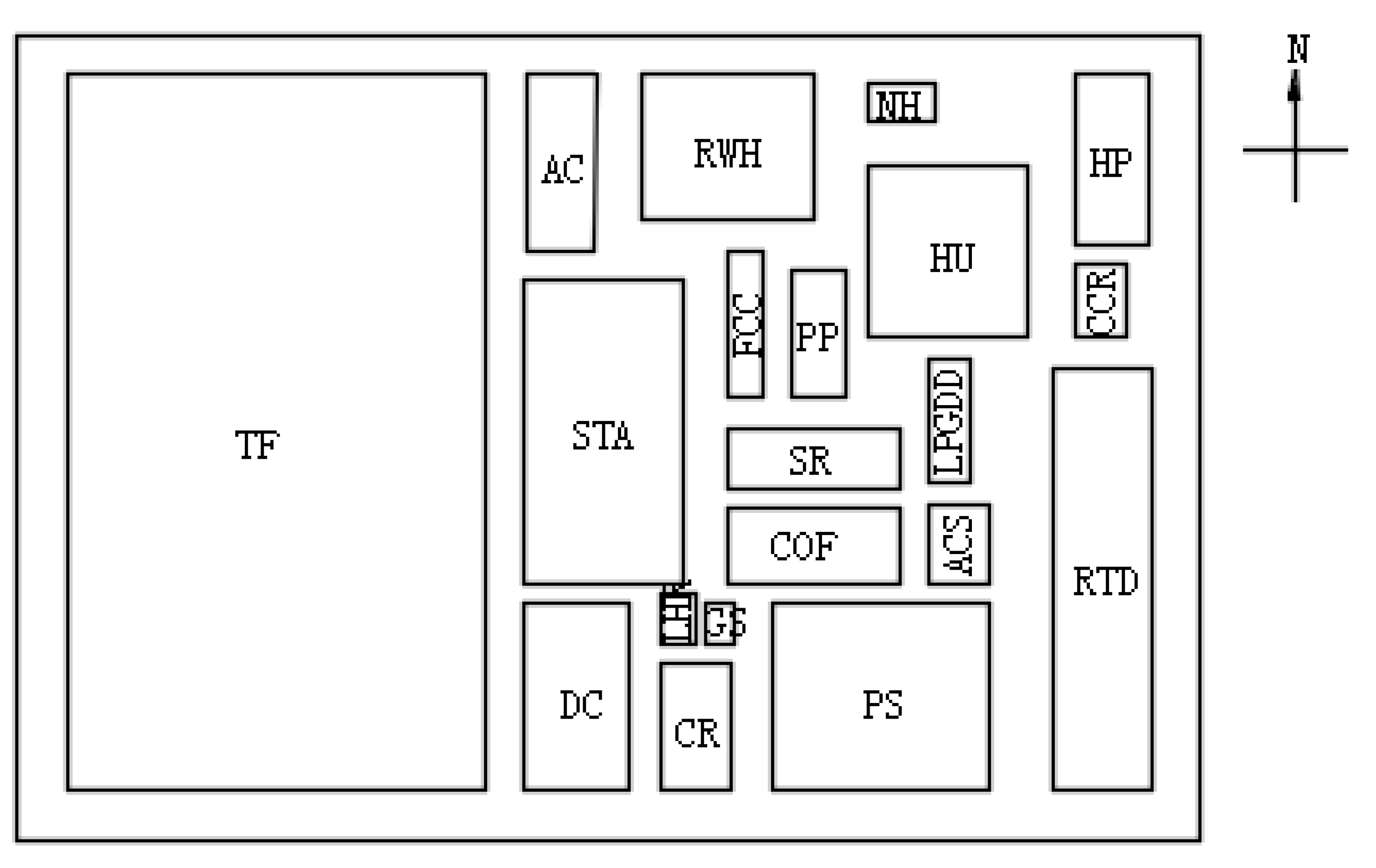
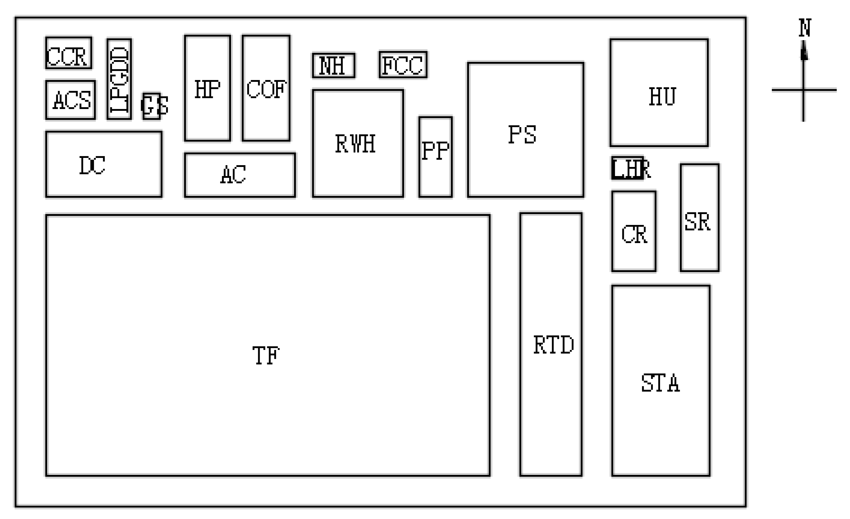
In this section, the key plant and other plants are optimized through coupling to figure out the effectiveness of the proposed methodology. With the initial sizes of all the plants and the sizes of the modified FCC plant, the industrial area is optimized with the objective of minimizing the total land cost. The original and modified industrial layout are, respectively, drawn in Figure 6 and Figure 7. The comparison of numerical results is represented in Table 4, which shows the respective and coupling results of the key plant and industrial area.
The modified key FCC plant with a new area and aspect ratio was coupled with the whole industrial layout, and the e of the FCC plant was calculated to be 4.58, indicating that the change in the key plant can effectively reduce the industrial area. Combined with Figure 6 and Figure 7 and Table 4, it can be seen that, for the key plant itself, the total annual cost after the reconstruction is 141,400 CNY/a higher than before. However, when the key plant is coupled with other plants to reach an area-wide layout, there is a significant reduction in the overall total industrial cost. The coupling cost after the modification is 1,947,500 CNY/a less than before, which is around 17 times the increased cost of the key plant itself. Combined with the two costs, the overall total cost of the industrial layout reduces by 1,806,100 CNY/a. Even though the key plant cost is higher after the modification due to the increase in PIC, POC, and FC, the total cost of the industrial area is still much lower. This is because after the modification, the changes of the area and aspect ratio lead to a better coupling of the key plant and other plants. A more compact area-wide layout is acquired and the land is used more efficiently, which greatly reduces the occupied area and saves the land cost. Compared with the increased cost of the key plant itself, the reduced cost of the whole industrial land is far greater and, therefore, the modified layout is obviously better. This indicates that the key plant surely has a significant impact on the area-wide layout. The plant modification and the slight increase in costs in the key plant may lead to a substantial reduction in the total costs of the area-wide layout, which can provide an idea for the design of an industrial park.
6. Conclusions
This paper proposes a new idea and a method regarding the layout problem. In previous studies, the correlation between the industrial area and a single plant has rarely been considered. To fill this gap, the coupling relationship of these two layout scales are focused on in this work, which will certainly lead to a better result. To reach a coupling layout planning, three steps of the optimization are carried out in sequence. The key plant with the greatest impact is selected according to the variable e. It is then modified in a multi-floor structure with plenty of constraints and the objective function, which is the total cost, including piping investment cost, pumping operating cost, land cost and floor construction cost. Both the cross-floor placement of towers and reactors and the constraints for the placement of specific facilities are considered. Finally, the original and modified key plant are separately optimized with other plants. The land cost is the objective function in the optimization of area-wide layout. Diagram and numerical comparisons are reached for the analysis of the coupling optimization. A refinery served as an example to verify the proposed methodology. A better solution was achieved. Case results show that even though the plant cost after the modification is 141,400 CNY/a higher, there is a 1,947,500 CNY/a reduction in the area-wide layout cost. When the key plant is coupled with the industrial area, the final total cost is reduced by 1,806,100 CNY/a, which turns out to be a significant improvement.
When studying the area-wide layout in the future, this method can be used to figure out the plant that has a greatest influence on the whole layout. The time value of money will be involved as well to reach a more valuable result. The internal modification of the key plant itself can bring great benefits to the whole industrial layout transformation, which saves resources and capital costs to a great extent. This method provides reference and a new direction for the retrofitting of a plant or a whole industrial area.
Author Contributions
The idea of coupled layout and optimization process is mainly raised by Y.W. The solving approach and case study are accomplished by Y.W. and S.X. Article writing and data extraction are mainly done by S.X. SRFA and the combination of algorithms are realized by H.Z. Guidance is provided by Y.W. and X.F. All authors have read and agreed to the published version of the manuscript.
Funding
Financial support from Science Foundation of China University of Petroleum, Beijing (No. 2462018BJC004) is gratefully acknowledged.
Conflicts of Interest
The authors declare no conflict of interest.
References
- Koopmans, T.C.; Beckmann, M. Assignment Problems and the Location of Economic Activities. Econometrica 1957, 25, 53–76. [Google Scholar] [CrossRef]
- Zhou, J.Y.; Love, P.E.D.; Teo, K.L.; Luo, H.B. An exact penalty function method for optimising QAP formulation in facility layout problem. Int. J. Prod. Res. 2017, 55, 2913–2929. [Google Scholar] [CrossRef]
- Kim, J.-G.; Kim, Y.-D. Layout planning for facilities with fixed shapes and input and output points. Int. J. Prod. Res. 2000, 38, 4635–4653. [Google Scholar] [CrossRef]
- Lee, G.-C.; Kim, Y.-D. Algorithms for adjusting shapes of departments in block layouts on the grid-based plane. Omega 2000, 28, 111–122. [Google Scholar] [CrossRef]
- Liu, J.; Liu, J. Applying multi-objective ant colony optimization algorithm for solving the unequal area facility layout problems. Appl. Soft. Comput. 2019, 74, 167–189. [Google Scholar] [CrossRef]
- Kalita, Z.; Datta, D. Multi-Objective Optimization of the Multi-Floor Facility Layout Problem; IEEE: New York, NY, USA, 2017; pp. 64–68. [Google Scholar]
- Chang, C.-H.; Lin, J.-g.; Lin, H.-J. Multiple-Floor Facility Layout Design with Aisle Construction. Ind. Eng. Manag. Syst. Int. J. 2006, 5, 1–10. [Google Scholar]
- Wang, R.Q.; Zhao, H.; Wu, Y.; Wang, Y.F.; Feng, X.; Liu, M.X. An industrial facility layout design method considering energy saving based on surplus rectangle fill algorithm. Energy 2018, 158, 1038–1051. [Google Scholar] [CrossRef]
- Wang, R.Q.; Wu, Y.; Wang, Y.F.; Feng, X. An industrial area layout optimization method based on dow’s Fire Explosion Index Method. Chem. Eng. Trans. 2017, 61, 493–498. [Google Scholar] [CrossRef]
- Wang, R.Q.; Wu, Y.; Wang, Y.F.; Feng, X.; Liu, M.X. An layout optimization method for industrial facilities based in domino hazard index. In Proceedings of the 9th International Conference on Foundations of Computer-Aided Process Design; Munoz, S.G., Laird, C.D., Realff, M.J., Eds.; Elsevier Science Bv: Amsterdam, The Netherlands, 2019; Volume 47, pp. 89–94. [Google Scholar]
- Xiao, Y.J.; Zheng, Y.; Zhang, L.M.; Kuo, Y.H. A combined zone-LP and simulated annealing algorithm for unequal-area facility layout problem. Adv. Prod. Eng. Manag. 2016, 11, 259–270. [Google Scholar] [CrossRef] [Green Version]
- Hou, S.W.; Wen, H.J.; Feng, S.X.; Wang, H.; Li, Z.B. Application of Layered Coding Genetic Algorithm in Optimization of Unequal Area Production Facilities Layout. Comput. Intell. Neurosci. 2019, 2019, 3650923. [Google Scholar] [CrossRef] [Green Version]
- Hu, M.H.; Wang, M.J. Using genetic algorithms on facilities layout problems. Int. J. Adv. Manuf. Technol. 2004, 23, 301–310. [Google Scholar] [CrossRef]
- Zhao, H.; Wang, Y.; Feng, X. Optimization of area-wide layout in petrochemical plant with multiple sets of facilities. Petrochem. Technol. 2017, 46, 938–943. [Google Scholar]
- Tari, F.G.; Neghabi, H. Constructing an optimal facility layout to maximize adjacency as a function of common boundary length. Eng. Optimiz. 2018, 50, 499–515. [Google Scholar] [CrossRef]
- Liu, J.F.; Zhang, H.Y.; He, K.; Jiang, S.Y. Multi-objective particle swarm optimization algorithm based on objective space division for the unequal-area facility layout problem. Expert Syst. Appl. 2018, 102, 179–192. [Google Scholar] [CrossRef]
- Feng, J.G.; Che, A. Novel integer linear programming models for the facility layout problem with fixed-size rectangular departments. Comput. Oper. Res. 2018, 95, 163–171. [Google Scholar] [CrossRef]
- Ahmadi, A.; Jokar, M.R.A. An efficient multiple-stage mathematical programming method for advanced single and multi-floor facility layout problems. Appl. Math. Model. 2016, 40, 5605–5620. [Google Scholar] [CrossRef]
- Anjos, M.F.; Vieira, M.V.C. An improved two-stage optimization-based framework for unequal-areas facility layout. Optim. Lett. 2016, 10, 1379–1392. [Google Scholar] [CrossRef] [Green Version]
- Leno, I.J.; Sankar, S.S.; Ponnambalam, S.G. An elitist strategy genetic algorithm using simulated annealing algorithm as local search for facility layout design. Int. J. Adv. Manuf. Technol. 2016, 84, 787–799. [Google Scholar] [CrossRef]
- Ebrahimi, A.; Kia, R.; Komijan, A.R. Solving a mathematical model integrating unequal-area facilities layout and part scheduling in a cellular manufacturing system by a genetic algorithm. SpringerPlus 2016, 5, 1254. [Google Scholar] [CrossRef] [Green Version]
- Vazquez-Roman, R.; Diaz-Ovalle, C.O.; Jung, S.; Castillo-Borja, F. A reformulated nonlinear model to solve the facility layout problem. Chem. Eng. Commun. 2019, 206, 476–487. [Google Scholar] [CrossRef]
- Kulturel-Konak, S. The zone-based dynamic facility layout problem. INFOR 2019, 57, 1–31. [Google Scholar] [CrossRef]
- Grobelny, J.; Michalski, R. A novel version of simulated annealing based on linguistic patterns for solving facility layout problems. Knowl. Based Syst. 2017, 124, 55–69. [Google Scholar] [CrossRef]
- Paes, F.G.; Pessoa, A.A.; Vidal, T. A hybrid genetic algorithm with decomposition phases for the Unequal Area Facility Layout Problem. Eur. J. Oper. Res. 2017, 256, 742–756. [Google Scholar] [CrossRef]
- Turanoglu, B.; Akkaya, G. A new hybrid heuristic algorithm based on bacterial foraging optimization for the dynamic facility layout problem. Expert Syst. Appl. 2018, 98, 93–104. [Google Scholar] [CrossRef]
- CCPS. Guidelines for Siting and Layout of Facilities, 2nd ed.; Wiley: New York, NU, USA, 2018; pp. 17–26. [Google Scholar]
- Ejeh, J.O.; Liu, S.S.; Papageorgiou, L.G. Optimal layout of multi-floor process plants using MILP. Comput. Chem. Eng. 2019, 131, 106573. [Google Scholar] [CrossRef]
- Latifi, S.E.; Mohammadi, E.; Khakzad, N. Process plant layout optimization with uncertainty and considering risk. Comput. Chem. Eng. 2017, 106, 224–242. [Google Scholar] [CrossRef]
- Lee, D.H.; Lee, C.J. The Plant Layout Optimization Considering the Operating Conditions. J. Chem. Eng. Jpn. 2017, 50, 568–576. [Google Scholar] [CrossRef]
- Elbeltagi, E.; Hegazy, T.; Eldosouky, A. Dynamic layout of construction temporary facilities considering safety. J. Constr. Eng. Manag. 2004, 130, 534–541. [Google Scholar] [CrossRef]
- Song, X.L.; Xu, J.P.; Zhang, Z.; Shen, C.; Xie, H.P.; Pena-Mora, F.; Wu, Y.M. Reconciling strategy towards construction site selection-layout for coal-fired power plants. Appl. Energy 2017, 204, 846–865. [Google Scholar] [CrossRef]
- Alves, D.T.S.; de Medeiros, J.L.; Araujo, O.D.F. Optimal determination of chemical plant layout via minimization of risk to general public using Monte Carlo and Simulated Annealing techniques. J. Loss Prev. Process Ind. 2016, 41, 202–214. [Google Scholar] [CrossRef]
- Dunker, T.; Radons, G.; Westkamper, E. A coevolutionary algorithm for a facility layout problem. Int. J. Prod. Res. 2003, 41, 3479–3500. [Google Scholar] [CrossRef]
- Jeong, D.; Seo, Y. Golden section search and hybrid tabu search-simulated anneling for layout design of unequal-sized facilities with fixed input and output points. Int. J. Ind. Eng. Theory Appl. Pract. 2018, 25, 297–315. [Google Scholar]
- Tavakkoli-Moghaddam, R. LADEGA: Unequal Facilities Layout Design Using a Genetic Algorithm for Large-Scale Problems; Stankin Publishing House: Moscow, Russia, 2000; pp. 237–243. [Google Scholar]
- Atta, S.; Mahapatra, P.R.S. Population-based improvement heuristic with local search for single-row facility layout problem. Sadhana Acad. Proc. Eng. Sci. 2019, 44, 222. [Google Scholar] [CrossRef] [Green Version]
- Stijepovic, M.Z.; Linke, P. Optimal waste heat recovery and reuse in industrial zones. Energy 2011, 36, 4019–4031. [Google Scholar] [CrossRef]
- Holland, J.H. Adaptation in Natural and Artificial Systems; University of Michigan Press: Ann Arbor, MI, USA, 1975. [Google Scholar]
- Pierreval, H.; Caux, C.; Paris, J.L.; Viguier, F. Evolutionary approaches to the design and organization of manufacturing systems. Comput. Ind. Eng. 2003, 44, 339–364. [Google Scholar] [CrossRef]
- Tao, W.; Wang, H.; Li, Z. Optimal Solution of Rectangular Part Layout Based on Rectangle-Filling Algorithm. China Mech. Eng. 2003, 14, 1104–1107. [Google Scholar]
Figure 1.
Algorithm flow diagram of proposed methodology.

Figure 2.
Average of e of each plant in two scenarios.

Figure 3.
Floor layout of modified FCC layout.

Figure 4.
Convergence curve of the hybrid algorithm.

Figure 5.
The cost comparison of original and reconstruction layout.

Figure 6.
Layout diagram with original fluidized catalytic cracking (FCC).

Figure 7.
Layout diagram with modified FCC.


Table 1.
Sizes and area of each plant.
| Number | Name | Length (m) | Width (m) | Area (m2) |
|---|---|---|---|---|
| 1 | PS | 205 | 234 | 47,970 |
| 2 | COF | 95 | 190 | 18,050 |
| 3 | GS | 37 | 59 | 2183 |
| 4 | HU | 176 | 190 | 33,440 |
| 5 | RWH | 165 | 190 | 31,350 |
| 6 | FCC | 74 | 186 | 13,764 |
| 7 | LHR | 59 | 44 | 2596 |
| 8 | LPGDD | 59 | 146 | 8614 |
| 9 | SR | 80 | 190 | 15,200 |
| 10 | AC | 196 | 88 | 17,248 |
| 11 | HP | 91 | 190 | 17,290 |
| 12 | CR | 88 | 146 | 12,848 |
| 13 | NH | 88 | 59 | 5192 |
| 14 | PP | 73 | 146 | 10,658 |
| 15 | DC | 124 | 205 | 25,420 |
| 16 | ACS | 99 | 80 | 7920 |
| 17 | CCR | 92 | 69 | 6348 |
| 18 | RTD | 117 | 439 | 51,363 |
| 19 | TF | 731 | 434 | 317,254 |
| 20 | STA | 176 | 322 | 56,672 |
Table 2.
e value of each plant.
| Number | Name | Area Changes Aspect Ratio Stays the Same | Area Changes Aspect Ratio Changes | ||||||
|---|---|---|---|---|---|---|---|---|---|
| 20% | 40% | 60% | 80% | 20% | 40% | 60% | 80% | ||
| 1 | PS | 1.10 | 1.46 | 1.76 | 1.89 | 1.20 | 1.18 | 1.76 | 1.71 |
| 2 | COF | 2.13 | 1.80 | 2.13 | 1.14 | 1.56 | 1.80 | 2.13 | 1.14 |
| 3 | HU | 1.26 | 1.53 | 2.22 | 2.15 | 1.26 | 1.69 | 1.41 | 2.45 |
| 4 | RWH | 1.35 | 1.14 | 1.55 | 2.94 | 1.27 | 1.36 | 1.55 | 2.94 |
| 5 | FCC | 2.70 | 3.23 | 4.28 | 5.21 | 2.70 | 3.48 | 4.84 | 7.07 |
| 6 | LPGDD | 2.68 | 3.17 | 4.16 | 2.38 | 2.08 | 2.38 | 3.57 | 2.38 |
| 7 | SR | 2.19 | 1.80 | 2.19 | 2.70 | 1.35 | 1.80 | 2.28 | 3.62 |
| 8 | AC | 1.41 | 1.88 | 2.23 | 4.46 | 2.08 | 1.58 | 2.23 | 2.08 |
| 9 | HP | 1.93 | 1.38 | 1.63 | 2.98 | 1.41 | 1.78 | 2.22 | 4.15 |
| 10 | CR | 2.69 | 3.06 | 2.79 | 3.19 | 2.59 | 3.06 | 3.19 | 3.44 |
| 11 | NH | 2.96 | 3.95 | 1.97 | 3.95 | 4.44 | 3.29 | 1.97 | 3.95 |
| 12 | PP | 3.25 | 3.05 | 1.90 | 1.92 | 3.13 | 3.05 | 4.33 | 5.29 |
| 13 | DC | 1.66 | 1.55 | 1.81 | 2.82 | 1.86 | 1.95 | 2.82 | 3.63 |
| 14 | ACS | 3.07 | 2.59 | 2.59 | 2.59 | 3.07 | 4.10 | 4.53 | 4.53 |
| 15 | CCR | 4.24 | 3.77 | 2.83 | 3.23 | 3.63 | 3.77 | 3.63 | 3.23 |
| 16 | TF | 1.05 | 1.10 | 1.15 | 1.16 | 1.03 | 1.07 | 1.05 | 1.11 |
| 17 | STA | 1.06 | 1.24 | 1.49 | 1.72 | 1.29 | 1.18 | 1.49 | 1.27 |
Table 3.
Results comparison of original and modified FCC layout.
| Original Layout | Reconstruction Layout | |
|---|---|---|
| Length (m) | 34 | 42 |
| Width (m) | 146 | 76 |
| LC (104 ¥/a) | 49.57 | 32.15 |
| PIC (104 ¥/a) | 30.26 | 34.99 |
| POC (104 ¥/a) | 22.28 | 29.82 |
| FC (104 ¥/a) | 0 | 19.29 |
| TC (104 ¥/a) | 102.11 | 116.25 |
Table 4.
Results comparison of original and reconstruction FCC and industrial layout.
| Original Layout | Modified Layout | Difference between the Modified and Original Layout | Coupling Result | |
|---|---|---|---|---|
| FCC plant total annual cost (104 ¥/a) | 102.11 | 116.25 | 14.14 | −180.61 |
| Industrial annual cost (104 ¥/a) | 7492.75 | 7298.00 | −194.75 |
© 2020 by the authors. Licensee MDPI, Basel, Switzerland. This article is an open access article distributed under the terms and conditions of the Creative Commons Attribution (CC BY) license (http://creativecommons.org/licenses/by/4.0/).
Share and Cite
MDPI and ACS Style
Wu, Y.; Xu, S.; Zhao, H.; Wang, Y.; Feng, X. Coupling Layout Optimization of Key Plant and Industrial Area. Processes 2020, 8, 185. https://0-doi-org.brum.beds.ac.uk/10.3390/pr8020185
AMA Style
Wu Y, Xu S, Zhao H, Wang Y, Feng X. Coupling Layout Optimization of Key Plant and Industrial Area. Processes. 2020; 8(2):185. https://0-doi-org.brum.beds.ac.uk/10.3390/pr8020185
Chicago/Turabian StyleWu, Yan, Siyu Xu, Huan Zhao, Yufei Wang, and Xiao Feng. 2020. "Coupling Layout Optimization of Key Plant and Industrial Area" Processes 8, no. 2: 185. https://0-doi-org.brum.beds.ac.uk/10.3390/pr8020185
Note that from the first issue of 2016, this journal uses article numbers instead of page numbers. See further details here.