Performance Assessment of SWRO Spiral-Wound Membrane Modules with Different Feed Spacer Dimensions

Abstract

Reverse osmosis is the leading process in seawater desalination. However, it is still an energy intensive technology. Feed spacer geometry design is a key factor in reverse osmosis spiral wound membrane module performance. Correlations obtained from experimental work and computational fluid dynamics modeling were used in a computational tool to simulate the impact of different feed spacer geometries in seawater reverse osmosis spiral wound membrane modules with different permeability coefficients in pressure vessels with 6, 7 and 8 elements. The aim of this work was to carry out a comparative analysis of the effect of different feed spacer geometries in combination with the water and solute permeability coefficients on seawater reverse osmosis spiral wound membrane modules performance. The results showed a higher impact of feed spacer geometries in the membrane with the highest production (highest water permeability coefficient). It was also found that the impact of feed spacer geometry increased with the number of spiral wound membrane modules in series in the pressure vessel. Installation of different feed spacer geometries in reverse osmosis membranes depending on the operating conditions could improve the performance of seawater reverse osmosis systems in terms of energy consumption and permeate quality.

1. Introduction

Seawater desalination has become one of the main solutions to the worldwide problem of water scarcity. Among the available technologies, reverse osmosis (RO) is widely regarded as being the most efficient and reliable [1]. However, seawater RO (SWRO) is an intensive energy consumption process [2,3]. Optimizing the design and operation of SWRO desalination plants is one of the various ways to reduce the specific energy consumption ($SEC$) [4,5,6]. A key factor in this respect is the SWRO membrane technology that is used [7,8]. In spiral-wound membrane modules (SWMMs), the permeability coefficients have a significant impact on plant performance in terms of production and solute rejection [9,10]. Important efforts are being made to try to inhibit the effect of fouling on the permeability coefficients during plant operation by improving the pretreatment process [11] and increasing the resistance to fouling [12]. Another important characteristic of SWRO SWMMs is the feed spacer geometry (FSG) [13,14]. The FSG plays an important role in the concentration polarization (CP) phenomena and the pressure drop along the SWMMs [15,16,17].

In the optimal design and operation of SWRO systems, consideration of the water and solute permeability coefficients (A and B, respectively) in conjunction with the FSG is fundamental. Different optimal FSGs and different operation windows have been obtained for different A and B [14]. Several works have shown the impact of FSGs on the hydrodynamics in the feed channel of SWMMs, which affect other parameters. G. Schock and A. Miquel [18] obtained correlations for the friction factor ($\lambda$) and the Sherwood number ($Sh$) for RO membranes in a spiral-wound configuration through experimental work. $\lambda$ depends on the Reynolds number ($Re$) and on two correlative parameters, and $Sh$ depends on $Re$, the Schmidt number ($Sc$) and three correlative parameters. $Sh$ is associated to the mass transfer coefficient (k) and therefore to the polarization factor ($PF$). V. Geraldes et al. [19] changed the equation obtained for $\lambda$ by including other parameter ($K_{\lambda }$) in order to consider pressure gradients in the inlet of the pressure vessels (PVs) and SWMM fittings. This equation was used to simulate and optimize a medium-sized SWRO system. A. Abbas [20] used a different correlation for $\lambda$ but analogous to the previous one. This correlation was obtained in an earlier work [21] and for different membranes (ultrafiltration). The mentioned correlation require the use of $Re$ and three correlative parameters. It was used for the simulation of an industrial water desalination plant. In 2004, J. Schwinge et al. [22] used the equation obtained in a previous work [21] but a parameter was removed from the correlation. The aforementioned studies investigated the fouling effect in SWMMs by using computational fluid dynamics (CFD). These former works did not allow the use of diverse FSGs, which have different parameters ($\lambda$ and $Sh$ respectively) for the calculation of pressure drop and $PF$. C.P. Koutsou et al. [23] improved the previous works by putting forward different equations for the calculation of dimensionless pressure drop (proportional to $\lambda$), taking into consideration geometric characteristics of the feed spacers such as the ratio of the distance between parallel filaments and the filament diameter (L/d), the angle between the crossing filaments ($\beta$) and the flow attack angle ($\alpha$). In a subsequent work, C.P. Koutsou et al. [24] used the equation obtained by G. Schock and A. Miquel to calculate the $Sh$ for different FSGs. One of the main advantages of the correlations obtained by C.P. Koutsou et al. [24] is the applicability in full-scale RO systems due to the short computation time required for calculation, contrary to CFD. Usually, CFD studies are focused on the design of the FSGs itself rather than in their impact of existing FSGs on full-scale RO desalination plants [25,26,27,28]. A performance study of a RO process considering the pressure drop, CP phenomena and the shape of the filament was carried out by G. Guillen and E.M.V. Hoek [29]. The research was done by proposing a three-parameter correlation for $\lambda$ and the usual correlation for $Sh$. The mentioned authors did not consider different FSGs. A.H. Haidari et al. [13] assessed the performance of six commercial feed spacers focusing on pressure drop. The impact of the CP and RO membrane characteristics were not taken into consideration in that study. Other interesting work was carried out by the same research group [30], in this work, the effect of feed spacer orientation on hydraulic conditions was studied. Assessment of pressure drop results considering different attack angles was done, higher pressure losses were observed with flow attack angle of 45${}^{°}$ than 90${}^{°}$. The authors used a correlation similar to the proposed by G. Schock and A. Miquel [18] to determine $\lambda$.

Numerous studies have been published on the optimal design of RO systems. Yan-Yue Lu et al. [31] developed an optimization method for designing RO systems considering different feed concentrations and permeate specifications. The algorithm used by these authors allowed the integration of different SWMMs in the PV. The equations used for pressure losses and the mass transfer coefficient (k) were the same as used by A. Abbas [20]. A multi-objective optimization algorithm was developed by F. Vince et al. [32]. The method optimized the $SEC$ and permeate flux in relation to the cost of the permeate. Pressure losses were calculated by using an equation proposed by the membrane manufacturer. K.M. Sassi and I.M. Mujtaba [33] proposed optimization of the operation of an RO desalination process which used SWMMs by considering membrane fouling. The $SEC$ was optimized at a fixed permeate flow rate and quality. The correlation proposed by A.R. Dacosta [21] was used to estimate pressure losses and k. Y. Du et al. [34] proposed an optimization method considering both SWRO and brackish water RO desalination systems with SWMMs. They considered the correlation proposed by V. Geraldes et al. [19] for pressure loss estimation and the correlation proposed by A.R. Dacosta [21] for k estimation. A. Altaee [35] developed a computational model for the design and performance estimation of SWRO systems. Equations proposed by the membrane manufacturer for pressure losses and $PF$ were used in that work. The same equations were used by E. Ruiz-Saavedra et al. [36,37] in their development of a design method for brackish water RO systems. June-Seok Choi et al. [38] centered their work around the optimization of two-stage SWRO systems. Equations obtained in another published work [39] for pressure losses and k were used. A computational tool for designing brackish water RO systems with SWMMs was developed by A. Ruiz-García and I. Nuez [40]. This tool allowed the use of different FSGs, but simulations using different FSGs in brackish water RO SWMMs were not provided.

To evaluate the impact of the different FSGs in a full-scale PV with commercial SWRO SWMMs requires simple equations that can be used without the high computational requirements of CFD modeling. This is the main motive to use simple correlations such as those proposed by some mentioned authors [18,23,24] are needed. Another important matter that should be considered concerns the membrane permeability coefficients A and B. The values of A and B are key in the optimization of the performance of SWMMs considering different FSGs. In full-scale SWRO desalination plants, slight variations $SEC$ could have large repercussions on operation and maintenance costs. This paper aims to simulate a PV with full-scale SWRO SWMMs under a range of feed flow ($Q_{\mathrm{f}}$), feed pressure ($p_{\mathrm{f}}$) and feed concentration ($C_{\mathrm{f}}$) characteristics, considering different membrane permeability coefficients (A and B) and FSGs.

The following sections are the methodology where characteristics of the selected SWMMs, process modeling and calculation algorithm are described; results and discussion where the performance analysis of the considered PVs that contain SWMMs with different FSGs is presented; and finally the conclusions of this work including future research lines that should be taken into consideration from now on.

2. Methodology

Two SWRO SWMMs were considered, FILMTEC^™ SW30XLE-400 and FILMTEC^™ SW30XHR-400 from Dupont^®, Wilmington, Delaware, USA. The Water Application Value Engine (WAVE) software from Dupont^® company was employed to determine the coefficients A and B of the SWMMs under test conditions.

Table 1. SWRO membrane permeability coefficients under test conditions.

SWMM	${\mathit{A}}_0$ (m Pa−1 s−1)	B (m s−1)
FILMTEC™ SW30XLE-400	$3.71\times {10}^{-12}$	$1.93\times {10}^{-8}$
FILMTEC™ SW30XHR-400	$2.47\times {10}^{-11}$	$1.16\times {10}^{-8}$

shows the calculated coefficients A and B. These SWRO membranes were selected due to their different characteristics (high production (SW30XLE-400) and high rejection (SW30XHR-400)). The mentioned characteristics are key in the operation of full-scale SWRO desalination plants. Both characteristics are related, through the membrane permeability coefficients A and B, with the performance of the desalination process in terms of $SEC$ and permeate quality.

To carry out a comparative study of the two full scale SWRO membranes, PVs of 6–8 elements were simulated. A $C_{\mathrm{f}}$ range of between 32 and 45 kg m${}^{-3}$ of sodium chloride (NaCl) was used with feed flow ($Q_{\mathrm{f}}$) and feed pressure ($p_{\mathrm{f}}$) ranges from 3 to 16 ${\mathrm{m}}^3{\mathrm{h}}^{-1}$ and from 40 to 80 bar, respectively. The different FSGs studied by C.P. Koutsou et al. [23] were used. The solution-diffusion transport model [41,42,43], which presumes that the RO membrane does not have porous or imperfections, was utilized. This model is based on considering that each solvent and solute are dissolved in the membrane separately on the feed-brine side and then diffused in individual fluxes through the membrane under the effect of pressure and concentration gradients (Equations (1) and (2)). This is the most extended model and provides results close to the real behavior of RO systems for both seawater and brackish water [44]. The transport equations used the mean values of each SWRO SWMM, and pressure gradients in the permeate carrier as well as temperature changes along the SWRO SWMMs were disregarded. The solvent (permeate) flow is described by Equation (1) and the solute flow by Equation (2).

$$Q_{\mathrm{p}}=A·(\mathsf{\Delta }p-\mathsf{\Delta }\pi )·S_{\mathrm{m}}$$

(1)

where $Q_{\mathrm{p}}$ is the permeate flow, $\mathsf{\Delta }p$ is the pressure gradient across the membrane, $\mathsf{\Delta }\pi$ is the osmotic pressure gradient across the membrane and $S_{\mathrm{m}}$ is the active membrane surface.

$$Q_{\mathrm{s}}=B·\mathsf{\Delta }C·S_{\mathrm{m}}$$

(2)

where $Q_{\mathrm{s}}$ is the solute flow across the membrane, and $\mathsf{\Delta }C$ is the concentration gradient of solute on either side of the membrane.

Coefficient A (Equation (1)) was considered to depend on two variables (Equation (3)): feed temperature (T) and flow factor (related to fouling and operating time ($FF$)) [40]. The effect of the CP on coefficient A was not considered. As the RO SWMMs get fouled the $Q_{\mathrm{p}}$ decreases under a fixed $p_{\mathrm{f}}$ which means that the coefficient A decreases. $FF$ is an important parameter that affect the coefficient A due to fouling [45]. Various methods have been proposed to try to predict the value of this parameter [46]. This work regards a comparative study between using different FSGs in two different SWRO SWMMs. It was considered that the flow factor $FF$ was 1 (membrane without fouling). Usually, the $FF$ decreases with operating time as the SWMMs get fouled [45]. A T of 25 ${}^{°}$C was considered, so the temperature correction factor ($TCF$) had a value of 1.

$$A=A_0·TCF·FF$$

(3)

where $A_0$ is the initial value of A. The net driving pressure ($NDP$) depends on $p_{\mathrm{f}}$, pressure drop ($\mathsf{\Delta }{p}_{\mathrm{fb}}$), permeate pressure ($p_{\mathrm{p}}$), average osmotic pressure on the membrane surface (${\pi }_{\mathrm{m}}$) and average osmotic pressure of the permeate (${\pi }_{\mathrm{p}}$):

$$NDP=(\mathsf{\Delta }p-\mathsf{\Delta }\pi )=p_{\mathrm{f}}-\frac{\mathsf{\Delta }{p}_{\mathrm{fb}}}{2}-p_{\mathrm{p}}-{\pi }_{\mathrm{m}}+{\pi }_{\mathrm{p}}$$

(4)

$\mathsf{\Delta }{p}_{\mathrm{fb}}$ was calculated as follows [40,47]:

$$\mathsf{\Delta }{p}_{\mathrm{fb}}=\lambda ·L·\frac{{\rho }_{\mathrm{fb}}}{d_{\mathrm{h}}}\frac{v_{\mathrm{fb}}}{2}$$

(5)

$$d_{\mathrm{h}}=\frac{4\epsilon }{\frac{2}{h}+(1-\epsilon )\frac{8}{h}}$$

(6)

$${\rho }_{\mathrm{fb}}=498.4·M+\sqrt{\mathrm{248,400}+752.4·C_{\mathrm{fb}}·M}$$

(7)

where

$$M=1.0069-2.757\times {10}^{-4}·T$$

(8)

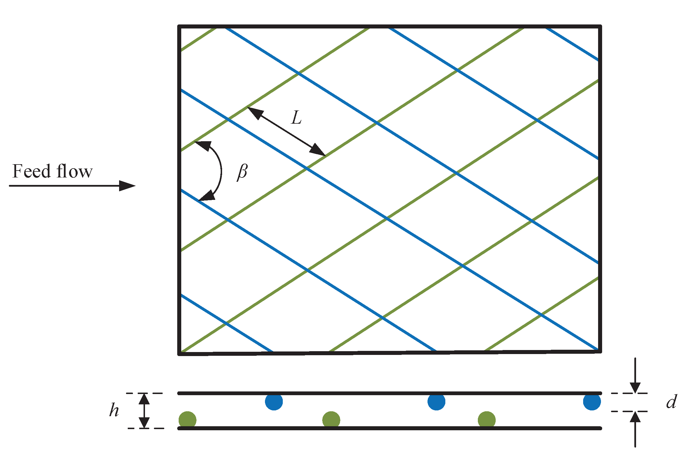
where L is the SWMM length (taken as 1 m), ${\rho }_{\mathrm{fb}}$ is the average feed-brine density ($\mathrm{k}\mathrm{g}{\mathrm{m}}^{-3}$), M is an empirical parameter, $v_{\mathrm{fb}}$ is the average feed-brine water velocity ($\mathrm{m}{\mathrm{s}}^{-1}$), $d_{\mathrm{h}}$ ($\mathrm{m}$) is the hydraulic diameter of the feed channel, $\epsilon$ is the porosity of the cross-sectional area of the feed channel (assumed 0.89 [18]) and h is the height of the feed channel, which was taken as $7.11\times {10}^{-4}$ m (28 milli-inches) for the two SWMMs. In this study, pressure losses in the permeate channel were not considered, and a value of $p_{\mathrm{p}}=\mathrm{34,473.8}$ Pa (5 psi) was considered [48]. Figure 1 shows the different FSG parameters. The correlations used for $\lambda$ were those proposed by C.P. Koutsou et al. [23] (

Table 2. Correlation for $\lambda$ calculation considering different FSGs [23].

	$\mathit{\beta }$ = 90${}^{°}$	$\mathit{\beta }$ = 105${}^{°}$	$\mathit{\beta }$ = 120${}^{°}$
$L/d$ = 6	$2.3{Re}^{-0.31}$	$2.2{Re}^{-0.23}$	$3.8{Re}^{-0.18}$
$L/d$ = 8	$0.8{Re}^{-0.19}$	$0.9{Re}^{-0.15}$	$1.2{Re}^{-0.14}$
$L/d$ = 12	$1.5{Re}^{-0.40}$	$1.1{Re}^{-0.31}$	$0.7{Re}^{-0.19}$

). $\lambda$ was multiplied by the parameter $K_{\lambda }$, which was introduced by V. Geraldes et al. [19]. Values between 1.9 and 2.9 were obtained in that study.

Due to CP phenomena, the solute concentration on membrane surface increases. This concentration generates a diffusive reverse flow to the feed-brine bulk. Once steady state conditions are established, the $PF$ provides the relationship between the average concentration of solute on the membrane surface ($C_{\mathrm{m}}$) and the average feed-brine solute concentration ($C_{\mathrm{fb}}$). Equation (12) was used to calculate ${\pi }_{\mathrm{p}}$. This enables calculation of the solute concentration of the permeate ($C_{\mathrm{p}}$) through Equation (9) [48]:

$$C_{\mathrm{p}}=B·PF·TCF·\frac{S_{\mathrm{m}}}{Q_{\mathrm{p}}}·\left(\frac{C_{\mathrm{f}}·(1+CF)}{2}\right)$$

(9)

$${\pi }_{\mathrm{m}}={\pi }_{\mathrm{f}}·\frac{C_{\mathrm{fb}}}{C_{\mathrm{f}}}·PF$$

(10)

$$CF=\frac{1}{1-Y}$$

(11)

where $CF$ is the concentration factor, ${\pi }_{\mathrm{f}}$ is the feedwater osmotic pressure and Y the fraction recovery of the SWMM. Equations (13) and (14) were obtained by using the film boundary model for CP [49].

$${\pi }_{\mathrm{f}}=4.54047·{\left({10}^3·C_{\mathrm{f}}/\left(M_{\mathrm{s}}·\rho \right)\right)}^{0.987}$$

(12)

$$C_{\mathrm{m}}=C_{\mathrm{fb}}·PF$$

(13)

$$PF=\frac{C_{\mathrm{m}}}{C_{\mathrm{fb}}}={\mathrm{e}}^{\frac{J_{\mathrm{p}}}{k}}$$

(14)

where $M_{\mathrm{s}}$ is the molecular weight of NaCl, $J_{\mathrm{p}}$ is the permeate flow per unit of $S_{\mathrm{m}}$ and k is the mass transfer coefficient, which is obtained by Equation (15) [18]:

$$Sh=a·{Re}^b·{Sc}^c=\frac{k·d_{\mathrm{h}}}{D}$$

(15)

$$Re=\frac{{\rho }_{\mathrm{fb}}·{\nu }_{\mathrm{fb}}·d_{\mathrm{h}}}{\eta }$$

(16)

$$Sc=\frac{\eta }{{\rho }_{\mathrm{fb}}·D_{\mathrm{s}}}$$

(17)

where a, b and c are parameters, $Sc$ is the Schmidt number, ${\nu }_{\mathrm{fb}}$ is the feed-brine velocity ($\mathrm{m}{\mathrm{s}}^{-1}$) and $\eta$ (0.000891 $\mathrm{k}\mathrm{g}{\mathrm{m}}^{-1}{\mathrm{s}}^{-1}$ when T = 25 ${}^{°}$C) the dynamic viscosity of pure water. C. P. Koutsou et al. [24] calculated correlations for the $Sh$ for different FSGs (

Table 3. Correlation for $Sh$ calculation considering different FSGs [24].

	$\mathit{\beta }$ = 90${}^{°}$	$\mathit{\beta }$ = 105${}^{°}$	$\mathit{\beta }$ = 120${}^{°}$
$L/d$ = 6	$0.14{Re}^{0.64}{Sc}^{0.42}$	$0.08{Re}^{0.715}{Sc}^{0.48}$	$0.073{Re}^{0.87}{Sc}^{0.45}$
$L/d$ = 8	$0.16{Re}^{0.605}{Sc}^{0.42}$	$0.17{Re}^{0.625}{Sc}^{0.42}$	$0.12{Re}^{0.71}{Sc}^{0.43}$
$L/d$ = 12	$0.26{Re}^{0.57}{Sc}^{0.37}$	$0.17{Re}^{0.64}{Sc}^{0.40}$	$0.19{Re}^{0.645}{Sc}^{0.38}$

). Solute diffusivity ($D_{\mathrm{s}}$ (${\mathrm{m}}^2{\mathrm{s}}^{-1}$)) was calculated using the Equation (18) [50]:

$$D_{\mathrm{s}}=(0.72598+0.023087T+0.00027657T^2)\times {10}^{-9}$$

(18)

In order to calculate all the above variables, an algorithm previously proposed by the authors [40] was used and implemented in MATLAB^®. The $SEC$ was determined by dividing the energy consumed by the high pressure pump (which was assumed to have 100% efficiency) by the permeate flow. Steps of 0.25 ${\mathrm{m}}^3{\mathrm{h}}^{-1}$, 0.5 bar and 1 kg m${}^{-3}$ were used for $Q_{\mathrm{f}}$, $p_{\mathrm{f}}$ and $C_{\mathrm{f}}$, respectively. If some result exceeded the constrains established by the membrane manufacturer (minimum concentrate flow of 3 ${\mathrm{m}}^3{\mathrm{h}}^{-1}$, 15% maximum element recovery), it was removed.

3. Results and Discussions

Figure 2 shows the flux recovery (R), $SEC$ and $C_{\mathrm{p}}$ of the FILMTEC^™ SW30XLE-400 and FILMTEC^™ SW30XHR-400 SWMMs installed in a PV with 7 elements, with a $C_{\mathrm{f}}$ = 32 kg m${}^{-3}$, $L/d$ = 6 and $\beta$ = 90${}^{°}$. The SW30XLE-400 has a higher coefficient A than the SW30XHR-400 (Table 1). Consequently, higher R values are reached with lower $p_{\mathrm{f}}$ than with the SW30XHR-400, but the operating window (possible operating points according with the membrane manufacturer constrains) is wider for the SW30XHR-400 than the SW30XLE-400 (Figure 2a,b). This is due to the high permeate production attained by the SW30XLE-400 membrane. As the pressure rises the concentrate flow decreases considerably, reaching the minimum established by the manufacturer with not very high pressures. This factor should be taken into account when this type of membrane is placed in PVs of 7 and 8 elements. Figure 2c,d show that low $SEC$ values were reached with $Q_{\mathrm{f}}$ values ranging between 5 and 10 ${\mathrm{m}}^3{\mathrm{h}}^{-1}$ for both membranes. The more elements arranged in series the higher the R and the lower the $SEC$ up to the point allowed by the minimum reject flow restriction imposed by the membrane manufacturer. The $C_{\mathrm{p}}$ decreased with increasing $Q_{\mathrm{f}}$ and $p_{\mathrm{f}}$ (Figure 2e,f) caused by coefficient B was constant, and the higher the $v_{\mathrm{fb}}$ the lower the $PF$ and $C_{\mathrm{m}}$. It should be remarked that changes in $C_{\mathrm{f}}$ and/or of the coefficients A and B (caused by fouling) could considerably vary the operating points values.

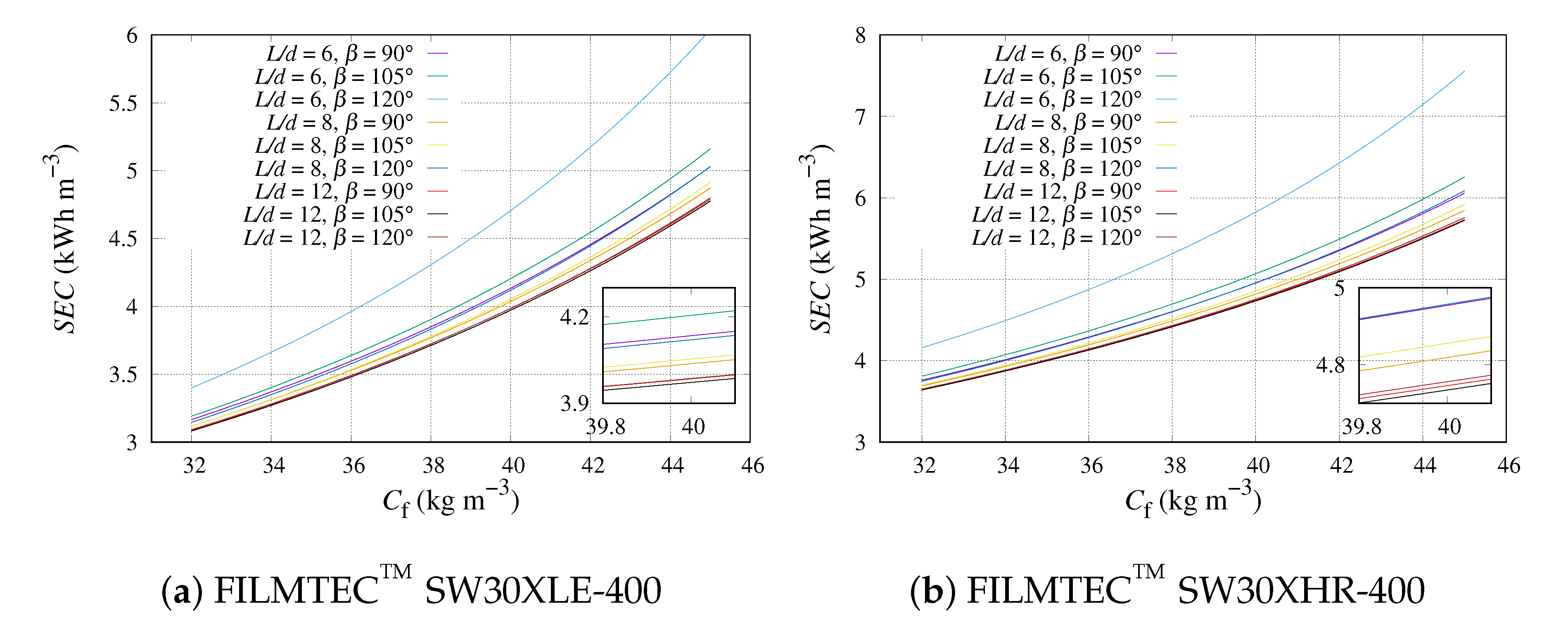
Figure 3a,b show the exponential growth of $SEC$ with the increase of $C_{\mathrm{f}}$. With the increment of $C_{\mathrm{f}}$ there was a small increase in the distance of the exponential curves of each FSG. The membrane with the higher coefficient A showed to have a lower $SEC$. Although, the separation between curves was more pronounced for the SW30XLE-400 than the SW30XHR-400 membrane. This showed that the influence of FSG with the $C_{\mathrm{f}}$ was higher for the SW30XHR-400 membrane. This was due to mentioned SWMM allowed to pass less salt (higher $C_{\mathrm{fb}}$) and spite of having lower coefficient A (which make $C_{\mathrm{fb}}$ to decrease), the impact of having lower coefficient B was higher than having a higher A on $SEC$.

As happened with $SEC$, $C_{\mathrm{p}}$ also showed an exponential growth with the increase of $C_{\mathrm{f}}$ for both membranes (Figure 4a,b). Again, slightly bigger differences between curves were reached at higher $C_{\mathrm{f}}$ values and were even more pronounced for the membrane with the higher coefficient A (SW30XLE-400). The $C_{\mathrm{p}}$ in the SW30XHR-400 was in a shorter range (0.1–0.25 kg m${}^{-3}$) than in the SW30XLE-400 (0.16–0.35 kg m${}^{-3}$). The response of the membrane with the lower B showed a more stable salt rejection for a range of $C_{\mathrm{f}}$.

Table 4. $SEC$ (kWh m${}^{-3}$) for PVs of 6 and 8 SWMMs with the two membranes studied with different FSGs.

Inputs	$\mathit{L}/\mathit{d}$	$\mathit{\beta }$	SW30XLE-400		SW30XHR-400
			$\mathit{SEC}(\mathbf{6}/\mathit{PV})$	$\mathit{SEC}(\mathbf{8}/\mathit{PV})$	$\mathit{SEC}(\mathbf{6}/\mathit{PV})$	$\mathit{SEC}(\mathbf{8}/\mathit{PV})$
$C_{\mathrm{f}}=35$$p_{\mathrm{f}}=55$$Q_{\mathrm{f}}=8$ (Case 1)	6	90${}^{°}$	3.2914	3.0479	3.8109	3.3649
		105${}^{°}$	3.2792	3.0495	3.8013	3.3692
		120${}^{°}$	3.3023	3.1034	3.8536	3.4544
	8	90${}^{°}$	3.2710	3.0247	3.7821	3.3328
		105${}^{°}$	3.2475	3.0154	3.7578	3.3222
		120${}^{°}$	3.2497	3.0246	3.7635	3.3356
	12	90${}^{°}$	3.2576	3.0132	3.7651	3.3172
		105${}^{°}$	3.2454	3.0073	3.7499	3.3089
		120${}^{°}$	3.2461	3.0084	3.7515	3.3107
$C_{\mathrm{f}}=35$$p_{\mathrm{f}}=55$$Q_{\mathrm{f}}=12$ (Case 2)	6	90${}^{°}$	3.9377	3.4803	4.9215	4.1484
		105${}^{°}$	3.9527	3.5170	4.9680	4.2153
		120${}^{°}$	4.1757	3.8070	5.3489	4.6777
	8	90${}^{°}$	3.8828	3.4181	4.8392	4.0583
		105${}^{°}$	3.8692	3.4221	4.8420	4.0760
		120${}^{°}$	3.8945	3.4608	4.8925	4.1396
	12	90${}^{°}$	3.8492	3.3844	4.7914	4.0095
		105${}^{°}$	3.8267	3.3729	4.7710	3.9986
		120${}^{°}$	3.8347	3.3816	4.7840	4.0123
$C_{\mathrm{f}}=40$$p_{\mathrm{f}}=60$$Q_{\mathrm{f}}=8$ (Case 3)	6	90${}^{°}$	3.6702	3.4173	4.1936	3.7382
		105${}^{°}$	3.6550	3.4180	4.1796	3.7411
		120${}^{°}$	3.6759	3.4737	4.2255	3.8268
	8	90${}^{°}$	3.6486	3.3924	4.1639	3.7045
		105${}^{°}$	3.6216	3.3815	4.1347	3.6917
		120${}^{°}$	3.6232	3.3911	4.1388	3.7051
	12	90${}^{°}$	3.6342	3.3799	4.1455	3.6878
		105${}^{°}$	3.6201	3.3730	4.1280	3.6784
		120${}^{°}$	3.6208	3.3741	4.1296	3.6803
$C_{\mathrm{f}}=40$$p_{\mathrm{f}}=60$$Q_{\mathrm{f}}=12$ (Case 4)	6	90${}^{°}$	4.3298	3.8614	5.3280	4.5324
		105${}^{°}$	4.3398	3.8973	5.3678	4.5964
		120${}^{°}$	4.5577	4.1918	5.7365	5.0555
	8	90${}^{°}$	4.2738	3.7965	5.2460	4.4405
		105${}^{°}$	4.2550	3.7985	5.2416	4.4544
		120${}^{°}$	4.2773	3.8374	5.2874	4.5164
	12	90${}^{°}$	4.2386	3.7606	5.1964	4.3895
		105${}^{°}$	4.2120	3.7471	5.1703	4.3754
		120${}^{°}$	4.2200	3.7561	5.1836	4.3892

,

Table 5. R (%) for PVs of 6 and 8 SWMMs with the two membranes studied with different FSGs.

Inputs	$\mathit{L}/\mathit{d}$	$\mathit{\beta }$	SW30XLE-400		SW30XHR-400
			$\mathit{R}(\mathbf{6}/\mathit{PV})$	$\mathit{R}(\mathbf{8}/\mathit{PV})$	$\mathit{R}(\mathbf{6}/\mathit{PV})$	$\mathit{R}(\mathbf{8}/\mathit{PV})$
$C_{\mathrm{f}}=35$$p_{\mathrm{f}}=55$$Q_{\mathrm{f}}=8$ (Case 1)	6	90${}^{°}$	46.42	50.13	40.09	45.40
		105${}^{°}$	46.59	50.10	40.19	45.35
		120${}^{°}$	46.26	49.23	39.65	44.23
	8	90${}^{°}$	46.71	50.51	40.40	45.84
		105${}^{°}$	47.04	50.67	40.66	45.99
		120${}^{°}$	47.01	50.51	40.59	45.80
	12	90${}^{°}$	46.90	50.70	40.58	46.06
		105${}^{°}$	47.08	50.80	40.74	46.17
		120${}^{°}$	47.06	50.78	40.72	46.15
$C_{\mathrm{f}}=35$$p_{\mathrm{f}}=55$$Q_{\mathrm{f}}=12$ (Case 2)	6	90${}^{°}$	38.80	43.90	31.04	36.83
		105${}^{°}$	38.65	43.44	30.75	36.24
		120${}^{°}$	36.59	40.13	28.56	32.66
	8	90${}^{°}$	39.35	44.70	31.57	37.65
		105${}^{°}$	39.49	44.64	31.55	37.48
		120${}^{°}$	39.23	44.15	31.23	36.91
	12	90${}^{°}$	39.69	45.14	31.89	38.10
		105${}^{°}$	39.92	45.30	32.02	38.21
		120${}^{°}$	39.84	45.18	31.94	38.08
$C_{\mathrm{f}}=40$$p_{\mathrm{f}}=60$$Q_{\mathrm{f}}=8$ (Case 3)	6	90${}^{°}$	45.41	48.77	39.74	44.59
		105${}^{°}$	45.60	48.76	39.88	44.55
		120${}^{°}$	45.34	47.98	39.44	43.55
	8	90${}^{°}$	45.68	49.13	40.03	44.99
		105${}^{°}$	46.02	49.29	40.31	45.15
		120${}^{°}$	46.00	49.15	40.27	44.98
	12	90${}^{°}$	45.86	49.31	40.20	45.19
		105${}^{°}$	46.04	49.41	40.37	45.31
		120${}^{°}$	46.03	49.40	40.36	45.29
$C_{\mathrm{f}}=40$$p_{\mathrm{f}}=60$$Q_{\mathrm{f}}=12$ (Case 4)	6	90${}^{°}$	38.49	43.16	31.28	36.77
		105${}^{°}$	38.40	42.77	31.05	36.26
		120${}^{°}$	36.57	39.76	29.05	32.97
	8	90${}^{°}$	39.00	43.90	31.77	37.53
		105${}^{°}$	39.17	43.88	31.80	37.42
		120${}^{°}$	38.97	43.43	31.52	36.90
	12	90${}^{°}$	39.32	44.32	32.07	37.97
		105${}^{°}$	39.57	44.48	32.24	38.09
		120${}^{°}$	39.49	44.37	32.15	37.97

and

Table 6. $C_{\mathrm{p}}$ (mg L${}^{-1}$ ) for PVs of 6 and 8 SWMMs with the two membranes studied with different FSGs.

Inputs	$\mathit{L}/\mathit{d}$	$\mathit{\beta }$	SW30XLE-400		SW30XHR-400
			${\mathit{C}}_{\mathbf{p}}(\mathbf{6}/\mathit{PV})$	${\mathit{C}}_{\mathbf{p}}(\mathbf{8}/\mathit{PV})$	${\mathit{C}}_{\mathbf{p}}(\mathbf{6}/\mathit{PV})$	${\mathit{C}}_{\mathbf{p}}(\mathbf{8}/\mathit{PV})$
$C_{\mathrm{f}}=35$$p_{\mathrm{f}}=55$$Q_{\mathrm{f}}=8$ (Case 1)	6	90${}^{°}$	202.25	276.78	126.36	165.82
		105${}^{°}$	200.62	275.85	125.24	165.07
		120${}^{°}$	198.64	275.67	124.40	165.51
	8	90${}^{°}$	201.83	276.11	125.91	165.11
		105${}^{°}$	199.75	274.69	124.44	163.91
		120${}^{°}$	199.26	274.61	124.11	163.85
	12	90${}^{°}$	201.22	275.53	125.44	164.58
		105${}^{°}$	200.36	275.00	124.72	164.01
		120${}^{°}$	200.34	274.99	124.72	164.02
$C_{\mathrm{f}}=35$$p_{\mathrm{f}}=55$$Q_{\mathrm{f}}=12$ (Case 2)	6	90${}^{°}$	144.12	188.30	97.70	121.18
		105${}^{°}$	143.02	188.03	97.49	121.59
		120${}^{°}$	145.55	194.55	101.53	129.40
	8	90${}^{°}$	143.22	186.81	96.71	119.61
		105${}^{°}$	141.56	185.61	95.94	119.11
		120${}^{°}$	141.28	185.95	96.14	119.82
	12	90${}^{°}$	142.46	185.84	96.03	118.67
		105${}^{°}$	141.16	184.78	95.22	117.94
		120${}^{°}$	141.26	184.95	95.36	118.16
$C_{\mathrm{f}}=40$$p_{\mathrm{f}}=60$$Q_{\mathrm{f}}=8$ (Case 3)	6	90${}^{°}$	234.03	320.34	145.60	192.05
		105${}^{°}$	232.25	319.40	144.30	191.23
		120${}^{°}$	230.17	319.52	143.22	191.76
	8	90${}^{°}$	233.54	319.52	145.11	191.26
		105${}^{°}$	231.25	318.01	143.43	189.93
		120${}^{°}$	230.72	317.98	143.04	189.88
	12	90${}^{°}$	232.86	318.86	144.58	190.66
		105${}^{°}$	231.90	318.27	143.76	190.04
		120${}^{°}$	231.87	318.27	143.76	190.05
$C_{\mathrm{f}}=40$$p_{\mathrm{f}}=60$$Q_{\mathrm{f}}=12$ (Case 4)	6	90${}^{°}$	165.92	217.90	111.30	139.09
		105${}^{°}$	164.60	217.59	110.92	139.42
		120${}^{°}$	167.02	224.61	114.84	147.42
	8	90${}^{°}$	164.96	216.23	110.28	137.42
		105${}^{°}$	163.04	214.90	109.31	136.77
		120${}^{°}$	162.65	215.29	109.41	137.46
	12	90${}^{°}$	164.13	215.13	109.54	136.38
		105${}^{°}$	162.63	213.95	108.57	135.53
		120${}^{°}$	162.74	214.14	108.73	135.76

show the results in terms of $SEC$, R and $C_{\mathrm{p}}$ in four different cases. Cases 1 and 2 with a standard $C_{\mathrm{f}}$ and Cases 3 and 4 with a high $C_{\mathrm{f}}$. Table 4 shows the $SEC$ for the two membranes studied in PVs of 6 and 8 SWMMs with different FSGs. The lowest $SEC$ for both membranes and PVs were obtained for $L/d$ = 12 and $\beta$ = 105${}^{°}$. As $Q_{\mathrm{f}}$ increased the differences between the aforementioned FSG and the rest in terms of $SEC$ grew wider. The highest values of $SEC$ were calculated for $L/d$ = 6 and $\beta$ = 120${}^{°}$ in both membranes. The difference between maximum and minimum $SEC$ was higher in PVs of 8 SWMMs in both membranes. The FSG had more impact on the SW30XHR-400, with greater differences between the maximum and minimum $SEC$ values than with the SW30XLE-400.

Table 5 shows the R for the two membranes studied in PVs of 6 and 8 SWMMs with different FSGs. The lowest R for both membranes and PVs were obtained for $L/d$ = 12 and $\beta$ = 105${}^{°}$ as in the $SEC$. The results obtained for R had the same trend as $SEC$ as both are closely related. Table 6 shows the $C_{\mathrm{p}}$ for the two membranes studied in PVs of 6 and 8 SWMMs with different FSGs. Considering the PVs of 6 SWMMs and Cases 1 and 3, the lowest $C_{\mathrm{p}}$ for the SW30XLE-400 were obtained for $L/d$ = 6 and $\beta$ = 120${}^{°}$, and for the SW30XHR-400 for $L/d$ = 8 and $\beta$ = 120${}^{°}$. When $Q_{\mathrm{f}}$ was increased, the minimum values of $C_{\mathrm{p}}$ were found in FSGs with $L/d$ = 12 and $\beta$ = 105${}^{°}$ for both membranes and PVs. In Cases 1 and 3, the highest values of $C_{\mathrm{p}}$ were obtained for $L/d$ = 6 and $\beta$ = 90${}^{°}$ in both membranes and PVs, while for Cases 2 and 4, the highest values of $C_{\mathrm{p}}$ were obtained for $L/d$ = 6 and $\beta$ = 120${}^{°}$ in both membranes and PVs. The difference between the maximum and minimum value of $C_{\mathrm{p}}$ was higher as $Q_{\mathrm{f}}$ was increased for both membranes and PVs.

Table 7. $\mathsf{\Delta }SEC$ (kWh m${}^{-3}$) between PVs of 6 and 7 ($\mathsf{\Delta }SEC(6-7)$), and 7 and 8 ($\mathsf{\Delta }SEC(7-8)$) SWMMs for the two membranes studied with different FSGs.

Inputs	$\mathit{L}/\mathit{d}$	$\mathit{\beta }$	SW30XLE-400		SW30XHR-400
			$\mathsf{\Delta }\mathit{SEC}(\mathbf{6}-\mathbf{7})$	$\mathsf{\Delta }\mathit{SEC}(\mathbf{7}-\mathbf{8})$	$\mathsf{\Delta }\mathit{SEC}(\mathbf{6}-\mathbf{7})$	$\mathsf{\Delta }\mathit{SEC}(\mathbf{7}-\mathbf{8})$
$C_{\mathrm{f}}=32$$p_{\mathrm{f}}=50$$Q_{\mathrm{f}}=8$ (Case 5)	6	90${}^{°}$	0.1567	0.1036	0.2784	0.1918
		105${}^{°}$	0.1491	0.0981	0.2711	0.1863
		120${}^{°}$	0.1316	0.0851	0.2540	0.1715
	8	90${}^{°}$	0.1582	0.1049	0.2800	0.1933
		105${}^{°}$	0.1507	0.0992	0.2733	0.1878
		120${}^{°}$	0.1467	0.0964	0.2693	0.1848
	12	90${}^{°}$	0.1573	0.1041	0.2794	0.1928
		105${}^{°}$	0.1537	0.1016	0.2760	0.1901
		120${}^{°}$	0.1536	0.1015	0.2759	0.1901
$C_{\mathrm{f}}=32$$p_{\mathrm{f}}=50$$Q_{\mathrm{f}}=12$ (Case 6)	6	90${}^{°}$	0.2830	0.1956	0.4612	0.3320
		105${}^{°}$	0.2718	0.1861	0.4504	0.3227
		120${}^{°}$	0.2330	0.1500	0.4015	0.2739
	8	90${}^{°}$	0.2868	0.1991	0.4660	0.3362
		105${}^{°}$	0.2782	0.1920	0.4581	0.3298
		120${}^{°}$	0.2711	0.1860	0.4511	0.3237
	12	90${}^{°}$	0.2873	0.1993	0.4666	0.3366
		105${}^{°}$	0.2819	0.1949	0.4618	0.3330
		120${}^{°}$	0.2815	0.1948	0.4612	0.3328
$C_{\mathrm{f}}=37$$p_{\mathrm{f}}=55$$Q_{\mathrm{f}}=8$ (Case 7)	6	90${}^{°}$	0.1617	0.1076	0.2857	0.1955
		105${}^{°}$	0.1527	0.1012	0.2770	0.1885
		120${}^{°}$	0.1322	0.0864	0.2559	0.1708
	8	90${}^{°}$	0.1637	0.1091	0.2879	0.1974
		105${}^{°}$	0.1548	0.1026	0.2798	0.1910
		120${}^{°}$	0.1501	0.0994	0.2747	0.1870
	12	90${}^{°}$	0.1628	0.1083	0.2872	0.1970
		105${}^{°}$	0.1586	0.1054	0.2829	0.1937
		120${}^{°}$	0.1583	0.1053	0.2829	0.1936
$C_{\mathrm{f}}=37$$p_{\mathrm{f}}=55$$Q_{\mathrm{f}}=12$ (Case 8)	6	90${}^{°}$	0.2916	0.1999	0.4786	0.3422
		105${}^{°}$	0.2778	0.1886	0.4650	0.3311
		120${}^{°}$	0.2334	0.1481	0.4118	0.2786
	8	90${}^{°}$	0.2964	0.2043	0.4838	0.3473
		105${}^{°}$	0.2859	0.1955	0.4745	0.3395
		120${}^{°}$	0.2769	0.1882	0.4659	0.3320
	12	90${}^{°}$	0.2971	0.2048	0.4849	0.3480
		105${}^{°}$	0.2902	0.1994	0.4788	0.3433
		120${}^{°}$	0.2896	0.1991	0.4784	0.3429

and

Table 8. $\mathsf{\Delta }{C}_{\mathrm{p}}$ (mg L${}^{-1}$) between PVs of 7 and 6 ($\mathsf{\Delta }{C}_{\mathrm{p}}(7-6)$), and 8 and 7 ($\mathsf{\Delta }{C}_{\mathrm{p}}(8-7)$) SWMMs for the two membranes studied with different FSGs.

Inputs	$\mathit{L}/\mathit{d}$	$\mathit{\beta }$	SW30XLE-400		SW30XHR-400
			$\mathsf{\Delta }{\mathit{C}}_{\mathbf{p}}(\mathbf{7}-\mathbf{6})$	$\mathsf{\Delta }{\mathit{C}}_{\mathbf{p}}(\mathbf{8}-\mathbf{7})$	$\mathsf{\Delta }{\mathit{C}}_{\mathbf{p}}(\mathbf{7}-\mathbf{6})$	$\mathsf{\Delta }{\mathit{C}}_{\mathbf{p}}(\mathbf{8}-\mathbf{7})$
$C_{\mathrm{f}}=32$$p_{\mathrm{f}}=50$$Q_{\mathrm{f}}=8$ (Case 5)	6	90${}^{°}$	32.44	33.86	17.04	17.86
		105${}^{°}$	32.77	34.19	17.21	18.05
		120${}^{°}$	33.74	35.12	17.90	18.80
	8	90${}^{°}$	32.29	33.73	16.89	17.72
		105${}^{°}$	32.56	34.03	16.98	17.84
		120${}^{°}$	32.78	34.22	17.12	17.98
	12	90${}^{°}$	32.27	33.74	16.83	17.67
		105${}^{°}$	32.42	33.88	16.88	17.74
		120${}^{°}$	32.43	33.89	16.89	17.75
$C_{\mathrm{f}}=32$$p_{\mathrm{f}}=50$$Q_{\mathrm{f}}=12$ (Case 6)	6	90${}^{°}$	19.28	20.11	10.52	10.74
		105${}^{°}$	19.71	20.59	10.88	11.13
		120${}^{°}$	22.07	23.21	13.11	13.65
	8	90${}^{°}$	18.93	19.76	10.18	10.39
		105${}^{°}$	19.13	20.00	10.33	10.56
		120${}^{°}$	19.47	20.36	10.62	10.87
	12	90${}^{°}$	18.78	19.63	10.02	10.24
		105${}^{°}$	18.86	19.74	10.05	10.28
		120${}^{°}$	18.90	19.78	10.10	10.32
$C_{\mathrm{f}}=37$$p_{\mathrm{f}}=55$$Q_{\mathrm{f}}=8$ (Case 7)	6	90${}^{°}$	38.36	39.81	20.45	21.40
		105${}^{°}$	38.79	40.21	20.67	21.64
		120${}^{°}$	40.00	41.35	21.51	22.56
	8	90${}^{°}$	38.16	39.63	20.27	21.22
		105${}^{°}$	38.52	39.99	20.40	21.38
		120${}^{°}$	38.79	40.23	20.58	21.57
	12	90${}^{°}$	38.14	39.63	20.21	21.17
		105${}^{°}$	38.32	39.80	20.29	21.25
		120${}^{°}$	38.34	39.81	20.29	21.26
$C_{\mathrm{f}}=37$$p_{\mathrm{f}}=55$$Q_{\mathrm{f}}=12$ (Case 8)	6	90${}^{°}$	23.09	24.06	12.59	12.90
		105${}^{°}$	23.61	24.64	13.00	13.34
		120${}^{°}$	26.28	27.59	15.39	16.05
	8	90${}^{°}$	22.68	23.63	12.22	12.51
		105${}^{°}$	22.94	23.96	12.39	12.71
		120${}^{°}$	23.35	24.39	12.72	13.06
	12	90${}^{°}$	22.49	23.47	12.04	12.34
		105${}^{°}$	22.62	23.63	12.08	12.40
		120${}^{°}$	22.67	23.67	12.13	12.45

show the results in terms of gradients of $SEC$ and $C_{\mathrm{p}}$ in four different cases. The $C_{\mathrm{f}}$ in these four cases represent the minimum and maximum values of the most common seawater concentrations (32 g L${}^{-1}$ for Cases 5 and 6, and 37 g L${}^{-1}$ for Cases 7 and 8). Table 7 shows the $SEC$ differences between PVs of 6–7 ($\mathsf{\Delta }SEC(6-7)$) and 7–8 ($\mathsf{\Delta }SEC(7-8)$) SWMMs of the SW30XLE-400 and SW30XHR-400 membranes, in different operating points. The highest differences were found in $\mathsf{\Delta }SEC(6-7)$ for both membranes. In all cases, wider differences corresponded to $\beta$ = 90${}^{°}$. Depending on the operating point and the membrane, the highest differences were obtained for $L/d$ = 8 and 12. For Case 5 (higher $Q_{\mathrm{f}}$) the highest differences were obtained in $L/d$ = 8 for the SW30XLE-400 and in $L/d$ = 12 for the SW30XHRE-400. This was due to different permeability coefficients and flow patterns (higher R for SW30XLE-400 implies lower $Q_{\mathrm{fb}}$ and $Re$). The higher the $Re$ the higher the $\mathsf{\Delta }{p}_{\mathrm{fb}}$ affecting R, $SEC$ and $C_{\mathrm{p}}$. This is the reason why differences in terms of $\mathsf{\Delta }SEC$ were higher for the SW30XHRE-400. Variations in $\mathsf{\Delta }SEC(6-7)$ (considering the 4 cases) of between 20.2 and 27.3% and of between 10.2 and 17.8% were obtained respectively for the SW30XLE-400 and SW30XHRE-400. $\mathsf{\Delta }SEC(7-8)$ variations of between 23.2 and 38.2% and between 12.7 and 24.9% were calculated for the SW30XLE-400 and SW30XHRE-400, respectively. In terms of $C_{\mathrm{p}}$, higher differences between PVs with 6 and 7 SWMMs and PVs with 7 and 8 elements were obtained for the SW30XHRE-400 than for the SW30XLE-400 (Table 8). This was due to the coefficient B of the SW30XHRE-400 membrane, which has a higher salt rejection. Consequently, $C_{\mathrm{m}}$ along the PV was higher (also affected by $PF$) for this membrane. Considering the 4 cases in terms of percentages, the variations of $\mathsf{\Delta }{C}_{\mathrm{p}}(7-6)$ and $\mathsf{\Delta }{C}_{\mathrm{p}}(8-7)$ were in a range of 4.6–17.5% and 6.3–30.9% for the SW30XLE-400 and in a range of 4.1–18.2% and 6.4–33.4% for the SW30XHRE-400. These percentages in terms of $\mathsf{\Delta }SEC$ and $\mathsf{\Delta }{C}_{\mathrm{p}}$ show the impact of FSGs considering different operating points (Cases) in three types of PV (6, 7 and 8 SWMMs).

4. Conclusions

The impact of different FSGs on SWRO membrane performance with different permeability coefficients was studied. It was observed that the longer the PV the higher the influence of the FSG on $SEC$. In terms of $SEC$, the membrane with a lower coefficient A suffered a more pronounced FSG impact. The effect of the FSG increased with $Q_{\mathrm{f}}$. The impact of the FSG on $C_{\mathrm{p}}$ was slightly higher for the membrane with the lower coefficient B and increased with $Q_{\mathrm{f}}$, with the differences between the maximum and minimum $C_{\mathrm{p}}$ values also increasing for both membranes. Manufacturers of RO SWMMs should take into consideration the installation of different FSGs in the same SWRO membranes. The option of having a membrane with different FSGs could help to improve SWRO plant operation. Normally, membrane manufacturers offer membranes with higher production or higher rejection (different permeability coefficients), different active area (400 or 440 ft${}^2$) or feed spacer thickness (28 or 34 milli-inches...) but with a default FSG. It should be noted that this work is based on simulations and that the impact of membrane fouling can have different effects on different FSGs. This aspect was not considered in this study. The decrease of the coefficient A with fouling and operating time as well as due to CP were also not considered as it could be different for each FSG and different operating conditions. In term of costs, it should be considered that manufacturing SWMMs with different FSGs on request could increase the investment cost of the RO system. Operating and maintenance costs regarding the application of different FSGs in SWMMs would depend on the performance decay due to fouling, which depend not only on operating conditions but on the FSGs.

References

- Qasim, M.; Badrelzaman, M.; Darwish, N.N.; Darwish, N.A.; Hilal, N. Reverse osmosis desalination: A state-of-the-art review. Desalination 2019, 459, 59–104. [Google Scholar] [CrossRef] [Green Version]
- Karabelas, A.J.; Koutsou, C.P.; Kostoglou, M.; Sioutopoulos, D.C. Analysis of specific energy consumption in reverse osmosis desalination processes. Desalination 2018, 431, 15–21. [Google Scholar] [CrossRef]
- Feo-García, J.; Ruiz-García, A.; Ruiz-Saavedra, E.; Melian-Martel, N. Energy consumption assessment of 4000 m3/d SWRO desalination plants. Desalin. Water Treat. 2016, 57, 23019–23023. [Google Scholar] [CrossRef]
- Voutchkov, N. Energy use for membrane seawater desalination—Current status and trends. Desalination 2018, 431, 2–14. [Google Scholar] [CrossRef]
- Kurihara, M.; Takeuchi, H. SWRO-PRO System in “Mega-ton Water System” for Energy Reduction and Low Environmental Impact. Water 2018, 10, 48. [Google Scholar] [CrossRef] [Green Version]
- Park, H.G.; Kwon, Y.N. Long-Term Stability of Low-Pressure Reverse Osmosis (RO) Membrane Operation—A Pilot Scale Study. Water 2018, 10, 93. [Google Scholar] [CrossRef] [Green Version]
- Zhao, D.L.; Japip, S.; Zhang, Y.; Weber, M.; Maletzko, C.; Chung, T.S. Emerging thin-film nanocomposite (TFN) membranes for reverse osmosis: A review. Water Res. 2020, 173, 115557. [Google Scholar] [CrossRef]
- Saleem, H.; Zaidi, S.J. Nanoparticles in reverse osmosis membranes for desalination: A state of the art review. Desalination 2020, 475, 114171. [Google Scholar] [CrossRef]
- Okamoto, Y.; Lienhard, J.H. How RO membrane permeability and other performance factors affect process cost and energy use: A review. Desalination 2019, 470, 114064. [Google Scholar] [CrossRef]
- Chen, C.; Qin, H. A Mathematical Modeling of the Reverse Osmosis Concentration Process of a Glucose Solution. Processes 2019, 7, 271. [Google Scholar] [CrossRef] [Green Version]
- Anis, S.F.; Hashaikeh, R.; Hilal, N. Reverse osmosis pretreatment technologies and future trends: A comprehensive review. Desalination 2019, 452, 159–195. [Google Scholar] [CrossRef] [Green Version]
- Li, Y.; Yang, S.; Zhang, K.; Van der Bruggen, B. Thin film nanocomposite reverse osmosis membrane modified by two dimensional laminar MoS2 with improved desalination performance and fouling-resistant characteristics. Desalination 2019, 454, 48–58. [Google Scholar] [CrossRef]
- Haidari, A.H.; Heijman, S.G.J.; van der Meer, W.G.J. Effect of spacer configuration on hydraulic conditions using PIV. Sep. Purif. Technol. 2018, 199, 9–19. [Google Scholar] [CrossRef]
- Ruiz-García, A.; de la Nuez Pestana, I. Feed Spacer Geometries and Permeability Coefficients. Effect on the Performance in BWRO Spriral-Wound Membrane Modules. Water 2019, 11, 152. [Google Scholar] [CrossRef] [Green Version]
- Abid, H.S.; Johnson, D.J.; Hashaikeh, R.; Hilal, N. A review of efforts to reduce membrane fouling by control of feed spacer characteristics. Desalination 2017, 420, 384–402. [Google Scholar] [CrossRef] [Green Version]
- Haidari, A.H.; Heijman, S.G.J.; van der Meer, W.G.J. Optimal design of spacers in reverse osmosis. Sep. Purif. Technol. 2018, 192, 441–456. [Google Scholar] [CrossRef]
- Xie, P.; Murdoch, L.C.; Ladner, D.A. Hydrodynamics of sinusoidal spacers for improved reverse osmosis performance. J. Membr. Sci. 2014, 453, 92–99. [Google Scholar] [CrossRef]
- Schock, G.; Miquel, A. Mass transfer and pressure loss in spiral wound modules. Desalination 1987, 64, 339–352. [Google Scholar] [CrossRef]
- Geraldes, V.; Pereira, N.E.; de Pinho, M.N. Simulation and Optimization of Medium-Sized Seawater Reverse Osmosis Processes with Spiral-Wound Modules. Ind. Eng. Chem. Res. 2005, 44, 1897–1905. [Google Scholar] [CrossRef]
- Abbas, A. Simulation and analysis of an industrial water desalination plant. Chem. Eng. Process. 2005, 44, 999–1004. [Google Scholar] [CrossRef]
- Costa, A.D.; Fane, A.; Wiley, D. Spacer characterization and pressure drop modelling in spacer-filled channels for ultrafiltration. J. Membr. Sci. 1994, 87, 79–98. [Google Scholar] [CrossRef]
- Schwinge, J.; Neal, P.R.; Wiley, D.E.; Fletcher, D.F.; Fane, A.G. Spiral wound modules and spacers: Review and analysis. J. Membr. Sci. 2004, 242, 129–153. [Google Scholar] [CrossRef]
- Koutsou, C.P.; Yiantsios, S.G.; Karabelas, A.J. Direct numerical simulation of flow in spacer-filled channels: Effect of spacer geometrical characteristics. J. Membr. Sci. 2007, 291, 53–69. [Google Scholar] [CrossRef]
- Koutsou, C.P.; Yiantsios, S.G.; Karabelas, A.J. A numerical and experimental study of mass transfer in spacer-filled channels: Effects of spacer geometrical characteristics and Schmidt number. J. Membr. Sci. 2009, 326, 234–251. [Google Scholar] [CrossRef]
- Liang, Y.Y.; Toh, K.Y.; Weihs, G.A.F. 3D CFD study of the effect of multi-layer spacers on membrane performance under steady flow. J. Membr. Sci. 2019, 580, 256–267. [Google Scholar] [CrossRef]
- Toh, K.Y.; Liang, Y.Y.; Lau, W.J.; Weihs, G.A.F. 3D CFD study on hydrodynamics and mass transfer phenomena for SWM feed spacer with different floating characteristics. Chem. Eng. Res. Des. 2020, 159, 36–46. [Google Scholar] [CrossRef]
- Kavianipour, O.; Ingram, G.D.; Vuthaluru, H.B. Studies into the mass transfer and energy consumption of commercial feed spacers for RO membrane modules using CFD: Effectiveness of performance measures. Chem. Eng. Res. Des. 2019, 141, 328–338. [Google Scholar] [CrossRef]
- Wang, Y.; He, W.; Müller, J.D. Sensitivity analysis and gradient-based optimisation of feed spacer shape in reverse osmosis membrane processes using discrete adjoint approach. Desalination 2019, 449, 26–40. [Google Scholar] [CrossRef]
- Guillen, G.; Hoek, E.M. Modeling the impacts of feed spacer geometry on reverse osmosis and nanofiltration processes. Chem. Eng. J. 2009, 149, 221–231. [Google Scholar] [CrossRef]
- Haidari, A.H.; Heijman, S.G.J.; Uijttewaal, W.S.J.; van der Meer, W.G.J. Determining effects of spacer orientations on channel hydraulic conditions using PIV. J. Water Process Eng. 2019, 31, 100820. [Google Scholar] [CrossRef]
- Lu, Y.Y.; Hu, Y.D.; Zhang, X.L.; Wu, L.Y.; Liu, Q.Z. Optimum design of reverse osmosis system under different feed concentration and product specification. J. Membr. Sci. 2007, 287, 219–229. [Google Scholar] [CrossRef]
- Vince, F.; Marechal, F.; Aoustin, E.; Bréant, P. Multi-objective optimization of RO desalination plants. Desalination 2008, 222, 96–118. [Google Scholar] [CrossRef]
- Sassi, K.M.; Mujtaba, I.M. Optimal design and operation of reverse osmosis desalination process with membrane fouling. Chem. Eng. J. 2011, 171, 582–593. [Google Scholar] [CrossRef]
- Du, Y.; Xie, L.; Wang, Y.; Xu, Y.; Wang, S. Optimization of Reverse Osmosis Networks with Spiral-Wound Modules. Ind. Eng. Chem. Res. 2012, 51, 11764–11777. [Google Scholar] [CrossRef]
- Altaee, A. Computational model for estimating reverse osmosis system design and performance: Part-one binary feed solution. Desalination 2012, 291, 101–105. [Google Scholar] [CrossRef]
- Saavedra, E.R.; Gotor, A.G.; Báez, S.O.P.; Martín, A.R.; Ruiz-García, A.; González, A.C. A design method of the RO system in reverse osmosis brackish water desalination plants (procedure). Desalin. Water Treat. 2013, 51, 4790–4799. [Google Scholar] [CrossRef]
- Ruiz-Saavedra, E.; Ruiz-García, A.; Ramos-Martín, A. A design method of the RO system in reverse osmosis brackish water desalination plants (calculations and simulations). Desalin. Water Treat. 2015, 55, 2562–2572. [Google Scholar] [CrossRef]
- Choi, J.S.; Kim, J.T. Modeling of full-scale reverse osmosis desalination system: Influence of operational parameters. J. Ind. Eng. Chem. 2015, 21, 261–268. [Google Scholar] [CrossRef]
- Avlonitis, S.A.; Pappas, M.; Moutesidis, K. A unified model for the detailed investigation of membrane modules and RO plants performance. Desalination 2007, 203, 218–228. [Google Scholar] [CrossRef]
- Ruiz-García, A.; de la Nuez-Pestana, I. A computational tool for designing BWRO systems with spiral wound modules. Desalination 2018, 426, 69–77. [Google Scholar] [CrossRef] [Green Version]
- Wijmans, J.G.; Baker, R.W. The solution-diffusion model: A review. J. Membr. Sci. 1995, 107, 1–21. [Google Scholar] [CrossRef]
- Al-Obaidi, M.A.; Kara-Zaitri, C.; Mujtaba, I.M. Scope and limitations of the irreversible thermodynamics and the solution diffusion models for the separation of binary and multi-component systems in reverse osmosis process. Comput. Chem. Eng. 2017, 100, 48–79. [Google Scholar] [CrossRef] [Green Version]
- Hinkle, K.R.; Wang, X.; Gu, X.; Jameson, C.J.; Murad, S. Computational Molecular Modeling of Transport Processes in Nanoporous Membranes. Processes 2018, 6, 124. [Google Scholar] [CrossRef] [Green Version]
- Kucera, J. Reverse Osmosis: Industrial Processes and Applications; John Wiley & Sons: Hoboken, NJ, USA, 2015. [Google Scholar]
- Ruiz-García, A.; Nuez, I. Long-term performance decline in a brackish water reverse osmosis desalination plant. Predictive model for the water permeability coefficient. Desalination 2016, 397, 101–107. [Google Scholar] [CrossRef] [Green Version]
- Ruiz-García, A.; Melián-Martel, N.; Nuez, I. Short Review on Predicting Fouling in RO Desalination. Membranes 2017, 7. [Google Scholar] [CrossRef] [Green Version]
- Du, Y.; Xie, L.; Liu, J.; Wang, Y.; Xu, Y.; Wang, S. Multi-objective optimization of reverse osmosis networks by lexicographic optimization and augmented epsilon constraint method. Desalination 2014, 333, 66–81. [Google Scholar] [CrossRef]
- Water, D.; Solutions, P. Filmtec Reverse Osmosis Membranes Technical Manual; Dow Water and Process Solutions: Midland, MI, USA, 2005. [Google Scholar]
- Mulder, M. Basic Principles of Membrane Technology; Springer Science & Business Media: Berlin/Heidelberg, Germany, 2012. [Google Scholar]
- Boudinar, M.; Hanbury, W.; Avlonitis, S. Numerical simulation and optimisation of spiral-wound modules. Desalination 1992, 86, 273–290. [Google Scholar] [CrossRef]
Figure 1.
Parameters of FSGs [14].
Figure 2.
, and of the two studied membranes with different permeability coefficients, PV with 7 SWMMs, = 32 kg m−3, = 6 and = 90.
Figure 3.
of a PV with 8 SWMMs in series considering different FSGs, a range of , = 55 bar and = 12 m3h−1.
Figure 4.
of a PV with 8 SWMMs in series considering different feed spacer geometries, a range of , = 55 bar and = 12 m3h−1.