Unconfined Dense Plunging Jets Used for Brine Disposal from Desalination Plants

Abstract

Laboratory experiments were conducted to measure entrained air bubble penetration depth and dilution of a dense vertical unconfined plunging jet to evaluate its performance as an outfall to dilute brine from desalination plants as well as a means to aerate water column. Experiments involved neutrally buoyant or dense plunging jets discharging in quiescent receiving water. The density difference between effluent and receiving water, the plunging jet length (height above water surface), and the receiving water salinity were varied in the experiments. Observed penetration depth for neutrally buoyant jets was somewhat greater than previously reported, and increased modestly with jet density. Increasing density also resulted in an increasing number of fine bubbles descending together with the dense plume. These observations can help guide the design of plunging jets to mitigate anoxic conditions in the water column when brine is introduced to a receiving water body, as with seawater desalination.

1. Introduction

This study is motivated by the potential use of plunging jets to dispose of reject desalination brine into Arabian Gulf (hereafter referred to as the Gulf) waters, in an effort to mitigate environmental impacts caused by brine discharges from Kuwait’s desalination plants. Brine discharge from desalination plants using reverse osmosis (RO) and multistage flash (MSF) distillation technologies may produce depressions in the dissolved oxygen (DO) level, and increased salinity and sea surface temperature (SST) [1,2]. In turn, these could potentially cause degradation of Kuwait’s marine diversity [3,4] both at the plant intakes and discharge outfalls [5] and further offshore [6,7].

With the Gulf Cooperation Council (GCC) countries’ desalination capacity estimated at 20 million m³/day of freshwater in 2012 [8], and with an estimated 2 m³ brine discharged per m³ of produced freshwater [9], the total volume of brine discharged into the Gulf from the GCC alone could be as high as 40 million m³/day. In the Gulf, 88% of the desalination plants operated by GCC countries use MSF and <10% use RO. Most of these desalination plants are located on the coast, and discharge brine into the near shore after mixing it partially with ambient seawater [3,10]. In Kuwait, contaminants from RO plants are discharged to the storm drains that eventually go to the Arabian Gulf; while from MSF plants, brine is discharged directly to the Arabian Gulf [11,12,13,14,15]. Very shallow coastal bathymetry, increased brine discharge, large distance from the limited flushing from the Indian Ocean, and reduced fresh water discharge from the nearby Shatt Al-Arab have made Kuwait’s marine waters the densest in the Gulf [16].

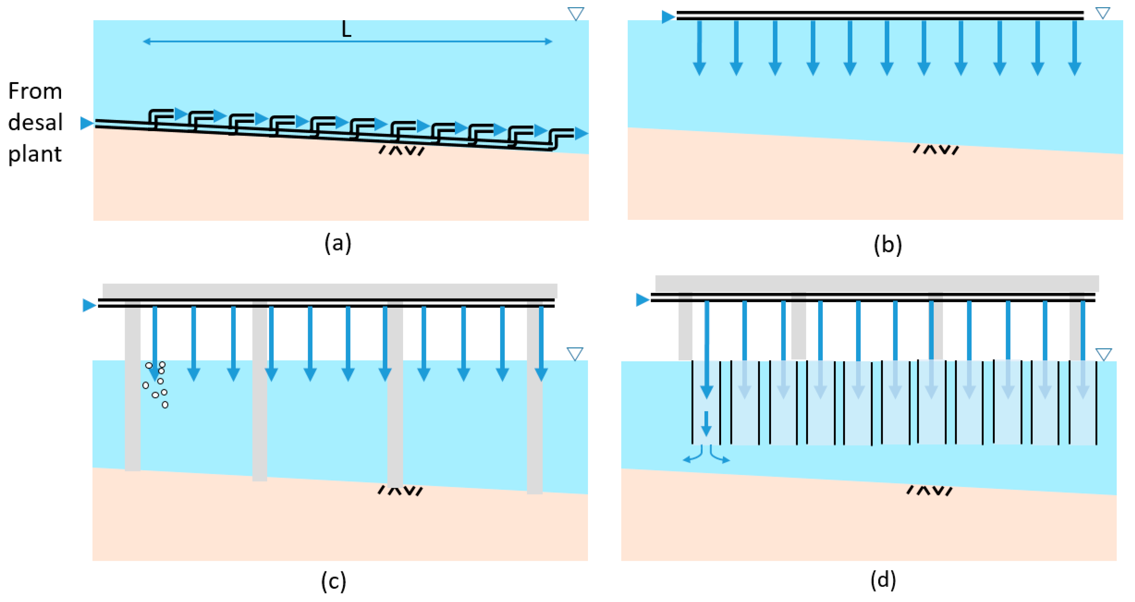
Reject brine discharges pose a risk of creating anoxic zones near discharge locations [7]. Therefore, it is worth exploring alternative engineering solutions that could combine the dilution of reject brine with reaeration from the surface. Figure 1 considers a pedagogic progression of four options for brine discharge: a) a bottom staged diffuser where dilution is achieved by jet momentum; b) a sinking dense plume caused by discharging brine from the water surface; c) unconfined plunging jets caused by discharging brine above the water surface; and d) confined plunging jets in which the release is shrouded by a downcomer.

Figure 1a shows a staged diffuser scheme that might be used to dilute thermal or wastewater effluent discharge in the receiving water body. The dilution ($S$) resulting from a staged diffuser of length $L$ is well studied and is dependent on the ambient current $u_a$, as well as the nozzle velocity $u_0$, as follows [17,18,19]:

$$S=\frac{\left(0.5u_a HL\right)}{Q_{0 }}+\sqrt{{\left(\frac{0.5u_a HL}{Q_0} \right)}^2+\frac{0.19HL{u}_0}{Q_0}},$$

(1)

where $H$ is the receiving water depth and $Q_0$ is the effluent discharge flowrate.

Picking a worst case ambient velocity of zero and using typical values for a desalination plant discharge of $Q_0=1$ m³/s (~20 million gallon per day), $u_0=4$ m/s, and $H$ = 3 m, the required diffuser length to achieve a target dilution of 20 (e.g., to reduce the excess salinity from ~40 psu to ~2 psu above ambient) is $L\approx 175$ m (Equation (1)).

Figure 1b shows a schematic of a line source of buoyancy released on the surface of a receiving water body, e.g., via a floating pipe. The discharge can be thought of as an upside down staged diffuser where the discharge is located on the water surface, and there is no horizontal momentum. For a weak ambient current (normalized ambient velocity $u_a^3/b_0\le 0.1$, where $b_0=Q_0\mathsf{\Delta }{\rho }_{0}g/{\rho }_{w}L$, is the buoyancy flux per unit length), and without ambient stratification, the dilution for a buoyant line source is [20,21]:

$$S=\frac{c_{1}H{b}_0^{1/3}}{q_0},$$

(2)

where $q_0=Q_0/L$ is the initial brine flowrate per unit length, $\mathsf{\Delta }{\rho }_0$ is the effluent density difference,${\rho }_w$ is the ambient water density, $g$ is the gravitational acceleration, $H$ is the ambient water depth, and $c_1$ is a proportionality constant reported as 0.27 by [20] for a finite length line source. To achieve a target near field dilution of 20, Equation (2) was used to predict the required diffuser length as $L\approx 225 m$.

Figure 1c depicts a line of dense plunging jets, similar to the outfall in Figure 1b, except that the ports are located at a fixed elevation above the surface, e.g., connected to a manifold supported by a pier. The plunging jet reactor concept has been in use for several decades, as a means of achieving high mass transfer rates by entraining gas bubbles into a liquid, at low capital and operating costs [22,23,24]. The typical objective is to contact the two phases to promote mass transfer. Plunging jet reactors are widely employed in a variety of processes, such as gas–liquid reactors in the chemical industry, aerobic wastewater treatment, air pollution abatement, froth flotation, and fermentation [25].

Figure 1d depicts an array of confined plunging liquid jet reactors (CPLJR), consisting of vertical confining tubes that are partially immersed in the liquid pool. The CPLJR is utilized to try to improve the mixing and mass transfer rates from the ambient air into the liquid. This can be achieved by: (1) increasing the jet penetration depth and (2) confining the bubbly jet region to increase the contact time between the gas and liquid [22,23].

Table 1. Oxygenation efficiency values of various aerators.

Aerator Type		OE (kg O2/kWh)
Diffused Air [26]	Fine bubble	1.2–2.0
	Coarse bubble	0.6–1.2
	Submerged jet	1.2–2.4
	Deep shaft [28]	3.0–6.0
	Static mixer [29]	1.2–1.8
Pure Oxygen [26]	UNOX	2.4–3.8
	VITOX	2.8–4.2
Mechanical [26]	Simcar surface aerator	2.1–2.4
	Turbine aerator	2.1–3.2
	Simple cone	2.0–2.6
Oxidation brushes [26]	Kessener brush	2.4–3.2
	Cage rotor	1.4–3.0
Plunging jet (air–water) [27]	Unconfined systems	0.7–8.0
	Confined systems	0.3–4.0
	Bioreactor [30]	2.0–4.6

(modified from [26,27]) shows the oxygen transfer efficiencies (defined as the mass of oxygen introduced to a reactor system per kWh of energy expenditure) reported for a range of aeration technologies. As seen from Table 1, plunging jet reactors (both confined and unconfined) are capable of achieving oxygen efficiencies comparable to other conventional aeration technologies.

Because plunging jets were historically focused on enhancing mass transfer from the gas phase to a single liquid phase, the vast majority of previous studies are performed with neutrally buoyant jets, i.e., the jet and the receiving water are of the same density [31,32,33]. Some statistical studies have been performed for plunging jets of neutral buoyancy [34], and numerical and experimental work has been performed for a plunging jet of a smaller density than the ambient [35], but there is a lack of literature available for plunging jets with higher density than the receiving water.

There is also a lack of available measurements of the dilution capacity created by a plunging jet when discharged either unconfined or confined into a receiving water body. The main objectives of this paper, therefore, are to assess the effect of density difference (created by brine jets of varying salinity) on the behavior of a plunging jet, as well as measure the dilution capability of a dense plunging jet to see if it is comparable to the dilution capability of submerged or surface discharges. This study offers a schematic model for the calculation of the increase in dissolved oxygen concentration in the water column as a result of the use of an unconfined plunging jet. These estimates may inform the design of plunging jet reactors for desalination brine discharge that are optimized to attain maximum brine dilution and DO dissolution from the atmosphere. This study focuses on unconfined plunging jet reactors (Figure 1c), but future effort will include confined plunging jet reactors.

Plunging Jet Behavior

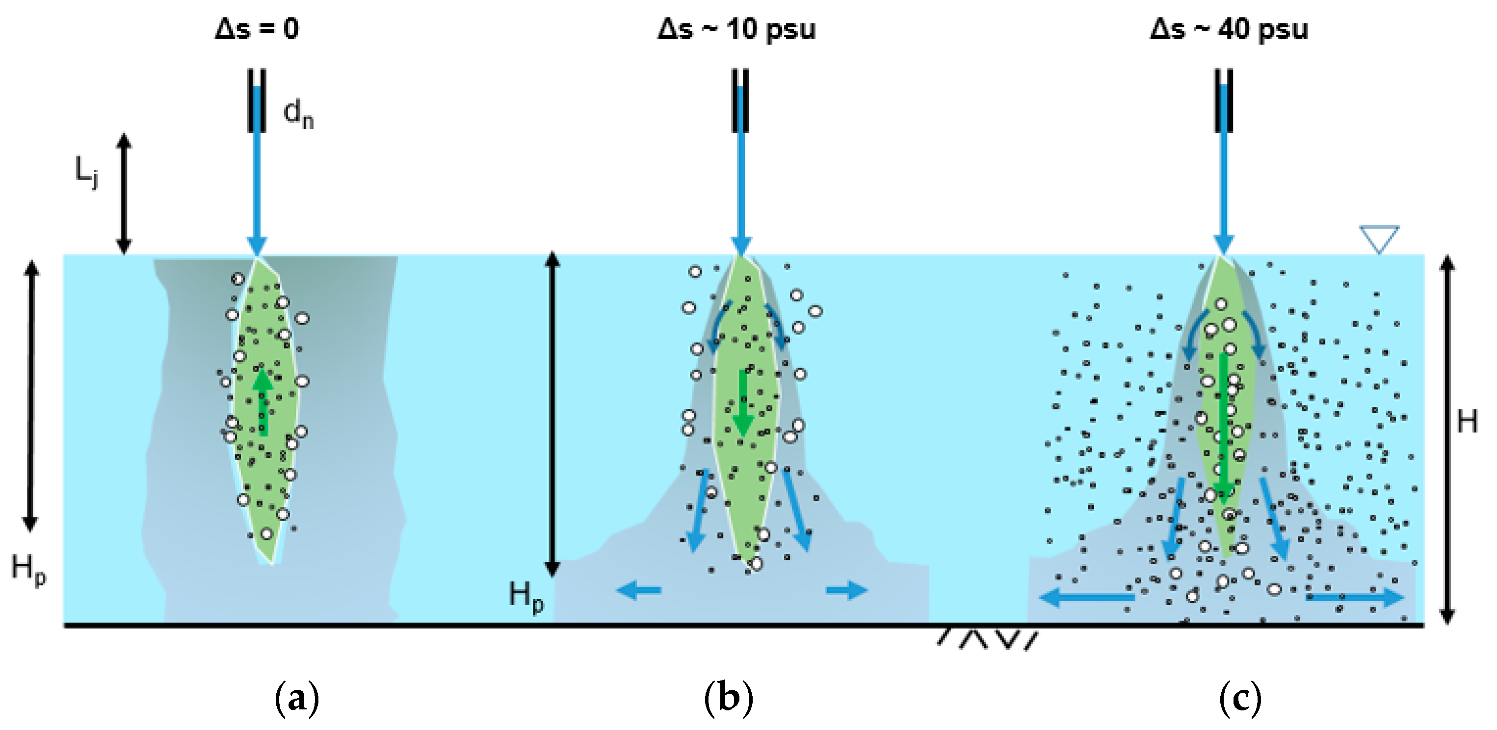
The above discussion treated a row of buoyant jets as a line source. Of course, a diffuser is comprised of individual jets, so the analysis starts with a single (unconfined) liquid jet. As shown in Figure 2, the jet plunges into an open liquid pool, creating a conical downflow dispersion of fine bubbles and a surrounding upflow of larger coalesced bubbles. Depending on the density difference between the effluent and receiving water, the fine bubbles may or may not reach the bottom. For cases in which the fine bubbles reach the bottom, they spread radially outwards with the diluted effluent flow, and then rise, forming an annulus wider than the annulus of large bubbles. The observed behavior of neutrally buoyant and dense plunging jets is described below.

When the vertical jet issues from the nozzle, the jet descends through the headspace over a vertical jet length $L_j$. There is a minimum jet descent velocity, known as the onset velocity, above which the headspace air begins to be entrained by the water jet. The onset velocity is dependent on the water density, water dynamic viscosity, surface tension between the air and water phase, turbulent velocity fluctuation, turbulent length scale, and the angle of the jet [25,36]. So far, there are no consistent predictions for the onset velocity; however, for vertical water jets, the onset velocities reported are in the range of 1.5–2.5 m/s [33,37,38].

Al-Anzi et al. [22] describes that increasing the jet length increases the amplitude of the disturbances on the surface of a rough jet, because these disturbances have a longer time to grow since their inception at the nozzle exit. The increased roughness, in turn, increases the rate of air entrainment into the jet prior to the jet hitting the water surface.

After breaking the surface of water, the impact momentum of the jet is responsible for carrying the two-phase jet/air mixture downward. For jets that have entrained air bubbles upon plunging into the receiving water body, the air bubbles descend a certain maximum distance (the penetration depth, denoted $H_p$) before their buoyancy drives them back to the water surface (Figure 2a,b). Numerous authors have observed the bubble penetration depth of neutrally buoyant plunging jets in water [25,33,38,39]. Bin [25] fit the following empirical relations for $H_p$ (in m) as a function of the nozzle velocity $V_0$ (in m/s) and the nozzle diameter $d_0$ (in m):

$$V_0{d}_0\text{<} 0.01:\hspace{1em}{H}_p=61{\left(V_0{d}_0\right)}^{1.36},$$

(3)

$$V_0{d}_0\text{≥} 0.01\text{:}\hspace{1em}{H}_p=2.4{\left(V_0{d}_0\right)}^{0.66}.$$

(4)

Note that the quantity $V_0{d}_0$ is related to the initial kinematic momentum of the jet as $M_0=\frac{\pi }{4}{\left(V_0{d}_0\right)}^2$. The proportionality constants in Equations (3) and (4) are dimensional as they incorporate a constant value for the density difference between the air and water phases. In this section, the dependence of $H_p$ is reframed using the jet kinematic momentum upon impact,$M_j=\frac{\pi }{4}{\left(V_j{d}_j\right)}^2$; the density ratio of the jet and receiving water body $\left(\frac{{\rho }_b}{{\rho }_w}\right)$; and gravitational constant $\left(g\right)$. Here, $V_j=\sqrt{V_0^2+2g{L}_j}$ (after [36]) and $d_j=\sqrt{V_0{d}_0{}^2/V_j}$ are the jet velocity and diameter at the water surface. For neutrally buoyant jets, $\frac{{\rho }_b}{{\rho }_w}=1$ and by dimensional analysis, the penetration depth of the bubbles in the receiving water should follow the relation:

$$H_p=\alpha {\left(\frac{M_j}{g}\right)}^{1/3},$$

(5)

where $\alpha$ is a proportionality constant determined to be $\alpha =4.0$ in the section below. For dense jets, $\frac{{\rho }_b}{{\rho }_w}>1$, and the following is presumed:

$$H_p=\alpha {\left(\frac{M_j}{g}\right)}^{1/3}\phi \left(\frac{{\rho }_b}{{\rho }_w}\right).$$

(6)

There exists a regime of dense brine plunging jets where the jet liquid buoyancy is sufficient to temporarily overcome the bubble’s positive buoyancy, pushing the bubbles to the bottom of the receiving water body (Figure 2c). In this case, the penetration depth of the bubbles is greater than the receiving water depth $\left(H\right)$. The bubbles, after reaching the bottom, travel radially outwards along with the dense jet liquid, and, once they are sufficiently far from the sinking plume core, they rise passively towards the water surface.

The plunging jet itself, whether or not it entrains air bubbles, is diluted as it mixes with the ambient receiving water body. Measurements of near field dilution of a plunging brine jet were compared with available literature (described below) for a dense jet released just below the water surface, or the inverted situation of a positively buoyant jet released at the bottom.

Chanson et al. [36] expressed the dilution at elevation $z$ of a round momentum jet discharging vertically upward into an unstratified ambient using the expression:

$$S=0.254\left(\frac{z}{l_Q}\right),$$

(7)

where $l_Q=Q_0/M_0^{0.5}$ is the volume length scale.

For a buoyancy dominated discharge, Tian et al. [21] developed a prediction for the dilution of a buoyant freshwater or low salinity wastewater discharge released just above the bottom of the sea floor into a saline ambient. The dilution at depth $H$ is given by:

$$S=0.26 B_o^{1/3} H^{5/3}/Q_o,$$

(8)

where $B_0=\frac{\mathsf{\Delta }{\rho }_0}{{\rho }_w}g{Q}_0$ is the initial buoyancy flux.

Fischer et al. [40], Section 9.2.3, discusses the dilution at elevation $z$ of an intermediate condition: a positively buoyant jet discharging vertically upward into an unstratified ambient. The dilution depends on two dimensionless parameters: $l_Q/l_M$ and $z/l_M$, and can be determined from Figure 8.7 from [40]. Here, $l_M$ is the momentum length scale defined as $M_0{}^{0.75}/B_0^{0.5}$.

2. Materials and Methods

The experimental setup for observing brine plunging jets is presented here. A water tank, at the Parsons Laboratory at MIT, of dimensions 4.9 m × 1.2 m × 0.6 m, filled with fresh or salt water to $H=$ 0.5 m depth, acts as the receiving water body. A submersible pump located in a separate brine reservoir (~140 L capacity) is able to deliver a steady liquid flowrate of up to 0.17 L/s downwards perpendicular to the water surface to form the vertical plunging jet. The discharge is dyed with Rhodamine WT and its concentration is measured using a Turner Designs Cyclops 7F model fluorometer.

In order to determine the dilution and aeration capability of these dense plunging jets, the following parameters were varied: the plunging jet length $L_j$ (the distance of the nozzle above the water surface); the density of the brine made with sodium chloride (expressed as $\mathsf{\Delta }s$, the difference in salinity between the effluent and the receiving water); and the density of the receiving water. The main experimental parameters were as follows: $\mathsf{\Delta }s$ = 0, 10, 40 psu and $L_j$ = 0, 0.15, 0.30, 0.60 m, resulting in a suite of 12 experimental runs with receiving water salinity ($s_w$) of zero. An additional set of 3 experiments with $\mathsf{\Delta }s$ = 0, 10, 40 psu and $L_j=0.30$ m were conducted with $s_w=$ 40 psu. In all of the experiments, a straight cylindrical nozzle was used with an internal diameter of $d_0$ = 10 mm, and a liquid flowrate of $Q_0=$ 163 cm³/s ($V_0=2.1$ m/s).

Table 2. Experimental parameters for unconfined plunging jet.

Run	$\Delta \mathit{s}\left(\mathbf{psu}\right)$	${\mathit{s}}_{\mathit{w}}\left(\mathbf{psu}\right)$	${\mathit{\rho }}_{\mathit{b}}(\mathbf{kg}/{\mathbf{m}}^3)$	${\mathit{\rho }}_{\mathit{w}}(\mathbf{kg}/{\mathbf{m}}^3)$	${\mathit{L}}_{\mathit{j}}\left(\mathbf{cm}\right)$	$\mathit{F}{\mathit{r}}_{\mathit{j}}$	${\mathit{H}}_{\mathit{p},\mathit{p}\mathit{r}\mathit{e}\mathit{d}}{}^{\mathit{a}}\left(\mathbf{cm}\right)$	${\mathit{H}}_{\mathit{p},\mathit{m}\mathit{e}\mathit{a}\mathit{s}}\left(\mathbf{cm}\right)$	$\mathit{W}$	${\mathit{S}}_{\mathit{H},\mathit{p}\mathit{r}\mathit{e}\mathit{d}}$	${\mathit{S}}_{\mathit{H},\mathit{m}\mathit{e}\mathit{a}\mathit{s}}$	${\mathit{S}}_{\mathit{R},\mathit{m}\mathit{e}\mathit{a}\mathit{s}}$
1	0	0	998	998	0	44	13.0			14 b
2	10	0	1006	998	0	44	13.0			14 c	8 ± 1	17 ± 3
3	40	0	1029	998	0	44	13.0			16 c	8 ± 1	20 ± 4
4	0	0	998	998	15	84	14.2	19.5 ± 1.4	14.0 ± 1.4	16 b
5	10	0	1006	998	15	84	14.2	20.7 ± 1.5	16.4 ± 1.6	15 c		10 ± 2
6	40	0	1029	998	15	84	14.2	≥50	19.7 ± 3.0	17 c		14 ± 3
7	0	0	998	998	30	129	15.0	18.1 ± 1.4	15.3 ± 1.1	17 b
8	10	0	1006	998	30	129	15.0	18.6 ± 1.5	14.8 ± 1.7	17 c		11 ± 3
9	40	0	1029	998	30	129	15.0	≥50	16.6 ± 3.2	17 c		17 ± 3
10	0	0	998	998	60	228	16.2			20 b
11	10	0	1006	998	60	228	16.2			20 c	16 ± 4	22 ± 5
12	40	0	1029	998	60	228	16.2			20 c	18 ± 4	23 ± 4
13	0	40	1029	1029	30	129	15.0	21.5 ± 1.4	9.9 ± 1.1	17 b
14	10	40	1036	1029	30	129	15.0	≥50	20.7 ± 3.3	17 c		13 ± 4
15	40	40	1059	1029	30	129	15.0	≥50	23.7 ± 4.8	17 c		18 ± 3

^a calculated using Equation (5) with $\alpha =4.0$ ^b calculated using Equation (7). ^c calculated using Figure 8.7, Section 9.2.3 from [40].

shows the experimental parameters for all the experiments. The jet Froude number $\left(F{r}_j=V_j{}^2/g{d}_j\right)$ is also listed in Table 2.

The above experimental parameters can be scaled to prototype values using Froude scaling. Assuming a desalination plant with brine flowrate of 1 m³/s using 6 jets to discharge, a single plunging jet will have a flowrate of 0.167 m³/s. The volume ratio between the field prototype and lab is, thus, $Q_r=\frac{0.167 {\mathrm{m}}^3/\mathrm{s}}{163 {\mathrm{cm}}^3/\mathrm{s}}=1024$. By Froude scaling, with similar density differences between model and prototype, this is equivalent to a length scale ratio of $L_r=Q_r^{0.4}=16$ between the field prototype and the lab. Thus, the receiving water depth of 50 cm and nozzle diameter of 10 mm in the lab scale to prototype water depth of 8 m and prototype nozzle diameter of 16 cm. The lab jet lengths of 0, 15, 30, and 60 cm scale to 0, 2.4, 4.8, and 9.6 m, respectively, in the field.

Measurements were made of: (1) the penetration depth of the plunging jet ($H_p$, the maximum depth to which the entrained gas bubbles descend within the water column); and (2) dye concentration on the tank bottom at a radial distance from the source ($R$) of 0.5 m (i.e., equal to one water depth). For some experiments, additional dye concentration measurements were made at the impact point on the tank bottom (i.e., $R=0$). The measured concentrations were used to calculate the dilution on the tank bottom at $R=50$ cm ($S_R$) and dilution at the impact point on the tank bottom ($S_H$). $S_R$ was not measured for experiments with $\mathsf{\Delta }s=0$ because the plume took a long time to reach the measurement location. $H_p$ was not measured for experiments with $L_j=60$ cm.

2.1. Measurement of Bubble Penetration Depth

For the measurement of penetration depth and the width of the bubble plume, a camera was mounted to the side of the tank to image the plunging jet behavior below the water surface at 60 frames per second. Since the maximum depth of the bubbles fluctuates with time (with a period of about 1 s and amplitude of about 2 cm), an average of all of the observed maximum depths and maximum bubble widths over the duration of each experiment was computed, using a total of ~5000 frames per experimental run.

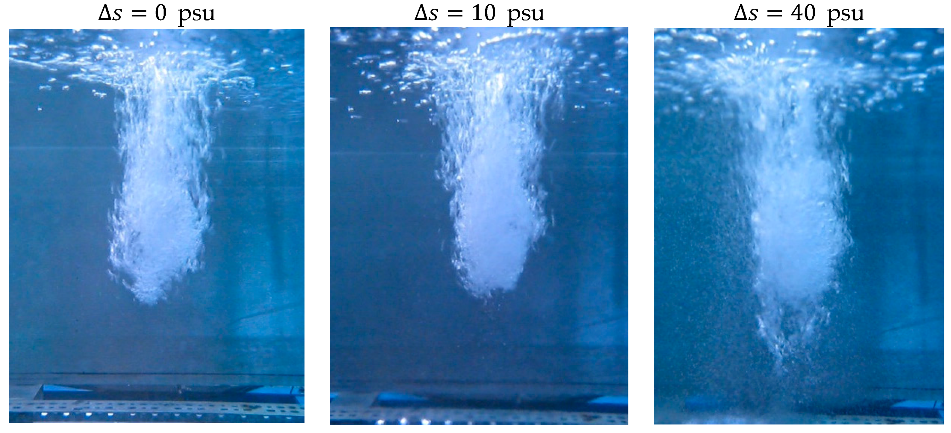
Figure 3 shows snapshots of movies taken of laboratory runs with $L_j=30$ cm. It can be observed from Figure 3 that small and large bubbles alike are plunged down to the penetration depth. For neutrally buoyant and moderately dense jets ($\mathsf{\Delta }s$= 0 and 10 psu), the bubbles were observed to plunge to about the same depths (range of 0.18–0.19 m; Table 2), similar to the predicted value of 0.19 m using Equation (3) [25]. However, for brine with $\mathsf{\Delta }s$ = 40 psu, while large bubbles behaved similarly to the neutrally buoyant plunging jet, smaller bubbles were pushed downwards to the bottom of the tank, spreading radially along the tank bottom before rising again up to the surface, resulting in larger $H_p$ and plume widths.

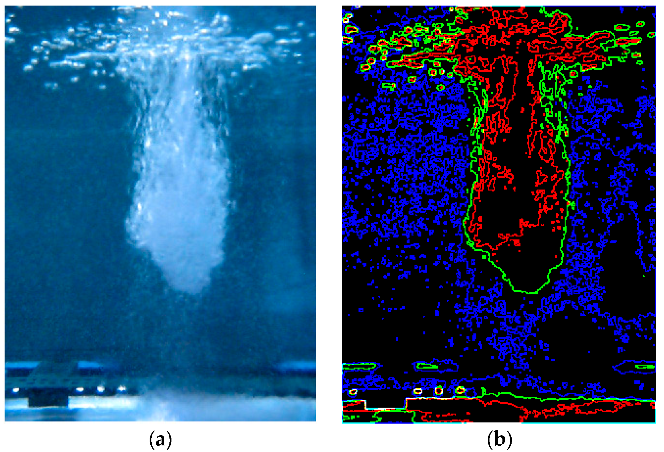
The penetration depth and width of the bubble plume were determined using image processing as follows. Each image of an experimental run was split into 3 separate images, each comprised of the red, green, and blue pixel intensities. MATLAB was used to apply an image filter that uses the Sobel operator to create a new image that exaggerates the edges present in each of the 3 images. The pixel intensities for each row of pixels were scanned from left to right, in the portion of the image that the plume is located (i.e., ignoring any bottom features as well as the bubbles on the water surface). Prior to each experimental run, an image of a ruler placed in the plane of the bubble plume centerline was taken in order to determine the conversion of image pixels to centimeters without the effect of parallax. The widest extent of the image edges (predominantly using the green image) was taken as $W$, the width of the bubble plume. The deepest extent of the image edge was taken as the bubble penetration depth $H_p$. See Figure 4 for an example of bubble plume width determination. Experimental results for the penetration depth are shown in Table 2.

2.2. Measurement of Dilution

For the measurement of dilution, dye concentration was measured using a fluorometer. Each experiment was run for a duration of 5–6 min with the fluorometer recording concentrations every second. Each experiment was also replicated (number of replicates = 2–5) and the reported dilution is the average of all the measurements after concentrations appeared to be quasi-steady. Measured dilutions are reported in Table 2. The variation in dilution indicated in Table 2 shows the standard deviation of all the concentration measurements. It can be seen from Table 2 that the measured dilutions are comparable to the predicted dilutions for jets discharged just below the water surface.

3. Results

The measurements of $H_p$ in Table 2 are plotted against ${\left(M_j/g\right)}^{1/3}$ in Figure 5, and compared with experiments from earlier literature (compiled by [25,33]) for the four experiments for which fine bubbles were not pushed to the bottom of the tank. The experimental data from this study (with $\frac{{\rho }_b}{{\rho }_w}>1$) is observed to be somewhat higher than the fitted curve for $\frac{{\rho }_b}{{\rho }_w}=1$. However, there were insufficient experiments with significant variation in the parameter ${\rho }_b/{\rho }_w$ to determine the form of function $\phi$ in Equation (6). Due to large variation, and the relatively small value of ${\left(M_j/g\right)}^{1/3}$ for the experiments, our curve fitting was limited to ${\left(M_j/g\right)}^{1/3}<0.125$ m. From Figure 5, the combined results yield a proportionality constant of $\alpha =4.0$, which was used for predictions of $H_p$ using Equation (5).

The presence of the bubbles in the bulk fluid serves to decrease the buoyancy of the descending plume. The bulk buoyancy of the descending buoyant jet is given by:

$$B=B_0+B_g=\frac{\mathsf{\Delta }{\rho }_0}{{\rho }_w}g{Q}_0+\frac{\mathsf{\Delta }{\rho }_g}{{\rho }_w}g{Q}_g,$$

(9)

where $\mathsf{\Delta }{\rho }_g$ is the density difference between the air and the ambient water, and $Q_g$ is the entrained gas flowrate.

An estimate of the maximum effect that the bubbles may have on the bulk buoyancy is to estimate the bulk jet buoyancy when all of the brine and the entrained bubbles are part of a single phase. The entrained gas volume rate for a plunging jet $\left(Q_g\right)$ is dependent on jet momentum, jet length, and perimeter (which, in turn, is dependent on the jet diameter). The empirical relation for an unconfined jet plunging vertically downward into an unconfined water body is [25,41]:

$$\frac{Q_g}{Q_0}=0.016{ [F{r}_j^{0.28}{\left(\frac{L_j}{d_0}\right)}^{0.4}]}^{1.17}=0.016 F{r}_j^{0.33}{\left(\frac{L_j}{d_0}\right)}^{0.47}.$$

(10)

Substituting Equation (10) into Equation (9) yields:

$$B=\frac{\mathsf{\Delta }{\rho }_0}{{\rho }_w}g{Q}_0 \left[1+0.016 \frac{\mathsf{\Delta }{\rho }_g}{\mathsf{\Delta }{\rho }_0}F{r}_j^{0.33}{\left(\frac{L_j}{d_0}\right)}^{0.47}\right].$$

(11)

Using values from the current experiments (for which $H_p$ was measured), the magnitude of the second term in the bracket of Equation (11) is in the range of 6 to 49 times the first term, i.e., the entrained air buoyancy is an order of magnitude greater than the buoyancy of the descending plume. This would indicate that if the entrained bubbles and the plunging brine jet were to act as a single phase, the jet would not sink. However, as the observations show the jets to sink, it is likely that only a small fraction of the entrained bubbles stays in a single phase with the plunging brine. The relative magnitudes of the positive buoyancy of the bubbles and negative buoyancy of the plume can also be used to explain the observed penetration depths. For experiments with $\mathsf{\Delta }s=10$ psu, the positive buoyancy due to the bubbles is much larger than the negative buoyancy of the plume. Thus, the bubbles are not carried to the bottom of the tank for such cases. However, for cases with $\mathsf{\Delta }s=40$ psu, the negative buoyancy of the plume is large enough to carry the bubbles to the bottom.

As discussed in the previous section, the current experimental parameters can be scaled to prototype parameters using Froude scaling. But this scaling does not apply to bubble size which depends on other parameters such as surface tension. The bubble size in the field can be estimated using a Weber number $\left(We={\rho }_w{V}_j^2{d}_j/\sigma \right)$ scaling. (Here, $\sigma$ is the surface tension and ${\rho }_w$ is the density of water). If the ratio of bubble size to nozzle diameter scales as $W{e}^{-0.6}$ [42], then the ratio of bubble diameter in the field to that in the lab is $L_r{}^{-0.2}$ (equal to 0.57 with $L_r=16$). Thus, the bubble diameter in the field is expected to be somewhat smaller than the bubble diameter observed in the lab.

Figure 6 shows the dilutions measured at $R=50$ cm ($S_R$) plotted against $\mathsf{\Delta }s$. These measurements are expected to be greater than $S_{H,pred}$ because the plume is allowed to spread and mix with the ambient water as a radial gravity current after impacting the bottom of the tank. $S_R$ increases slightly with increase in $\mathsf{\Delta }s$, and shows a non-monotonic dependence on $L_j$. As seen in Figure 6, dilution reduces as $L_j$ is increased from 0 to 15 cm, but increases as $L_j$ is increased further (for both values of $\mathsf{\Delta }s$). As shown in Table 2, $S_{H,pred}$ increases with increase in $L_j$ because the jet momentum used in the prediction increases. However, this trend is not replicated in $S_R$ because the jets lose some of the momentum upon impact at the water surface. The effect of receiving water salinity ($s_w$) can also be seen in Figure 6, with no significant difference seen in dilution for runs with $s_w=0$ and 40 psu ($L_j=30$ cm).

Dilutions measured at $R=0$ are plotted in Figure 7. As expected, the dilutions measured at $R=0$ are smaller than measurements at $R=50$ cm because they do not account for mixing after the plume hits the bottom (when it spreads radially). For $L_j=0$, the measured dilutions are lower than the predicted values at $z=H$ for a buoyant jet. This is likely due to the presence of a layer of diluted brine at the bottom which limits the entrainment of ambient water. For $L_j=60$ cm, the measured dilution is higher than that of a pure plume (discharge with zero momentum), but lower than the theoretical value for a jet with $L_j=60$ cm. This can be explained by: 1) the presence of layer of diluted brine; and 2) loss of momentum of the plunging jet after it hits the water surface. Note that the dilution of a pure plume is independent of $L_j$ (as it has no momentum).

4. Discussion

4.1. Aeration of Water Column

Al Anzi et al. [22] proposed the use of plunging liquid jet reactors, arranged in a diffuser array, to promote the aeration of the underlying water via entrainment of air bubbles from above the water surface. In this section, results from the current study are used to estimate the amount of aeration achievable with the bubbles entrained by plunging brine jets that are in contact with a moving water column. Consider the scenario in Figure 8, where a jet array of length $L$ comprising $n$ jets discharges vertically downward into a water column of depth $H$ where the ambient current is $u_a$. As the jets penetrate the water surface, they collectively entrain oxygen from the atmosphere into the water column at an oxygen flux rate of $Q_g=q_{g}L$, where $q_g$ is the gas flowrate per unit length of the jet array.

The increase in dissolved oxygen concentration in the water column ${\delta }_C{}_{DO}$ (mass/volume) can be calculated as the oxygen flux $J$ divided by the water flux, or:

$$\delta c_{DO}=\frac{J}{u_{a}HL}=\frac{Ak\left(c_s-c\right)}{u_{a}HL},$$

(12)

where $A=N\pi d^2$ is the total surface area of $N$ air bubbles (diameter $d$) in contact with the water column, $k$ the oxygen mass transfer coefficient, $c_s$ the saturation concentration of oxygen in water, and $c$ the dissolved oxygen concentration in water.

In turn, the number of bubbles in contact with the water can be estimated as equal to the bubble input rate $\left(\dot{N}\right)$ multiplied by the contact time $\left(t\right)$. If the bubbles are all of the same size, the bubble number rate in is given by $\frac{\pi d^3}{6}\dot{N}=Q_g=q_{g}L$. The contact time of the bubbles in the water column can be estimated by $t=H_p/u_b$, where $u_b$ is the bubble rise velocity. Substituting the above relations into Equation (12) yields:

$$\delta c_{DO}=\frac{N\pi d^{2}k\left(c_s-c\right)}{u_{a}HL}=\frac{6q_g{H}_{p}k\left(c_s-c\right)}{d{u}_b{u}_{a}H}.$$

(13)

Based on Equation (13) above, the aeration of the water column depends on the following four factors, each embodied by a variable present in the expression. Each of these four factors are discussed quantitatively for the plunging jet below.

A. The gas entrainment due to the plunging jet impinging across the water surface ($q_g$).

B. The bubble size distribution (and bubble velocity) due to the plunging jet ($u_b$ and $d$).

C. Depth of bubble penetration ($H_p$).

D. Mass transfer coefficient ($k$).

4.1.1. A. Gas Entrainment

The empirical relation for gas entrainment rate for an unconfined plunging jet is given by Equation (10). The range of applicability of Equation (10) is $L_j/d_0\le 100$, and $F{r}_j^{0.28}{\left(L_j/d_0\right)}^{0.4}\ge 10\text{.}$ For the current experiments where plunging jets were observed,$L_j/d_0=15-30$, and $F{r}_j^{0.28}{\left(L_j/d_0\right)}^{0.4}=10-14$, and therefore Equation (10) can be applied to predict their gas entrainment.

Miwa et al. [39] compiled many predictive formulas for the air entrainment rate for neutrally buoyant plunging jets, and also offered an empirical relation for the air entrainment rate as a function of the Laplace length scale $\left(La=\sqrt{\sigma /\mathsf{\Delta }{\rho }_{gb}g}\right)$ and the Weber number. However, the current experimental parameters are outside the range of applicability of their results.

4.1.2. B. Bubble Size Distribution and Rise Velocity

The size distribution of the bubbles created by the plunging jet determines both the total interfacial surface area across which the oxygen mass transfer can occur, and the contact time of the bubbles as they ultimately rise back to the surface from their maximum penetration depth.

The bubble shape depends on the Reynolds number, Eötvös number $Eo=g\mathsf{\Delta }{\rho }_{al}{d}^2/\sigma$ (ratio of buoyancy and surface tension), and the Morton number $M=g{\mu }^4\mathsf{\Delta }{\rho }_{gb}/{\rho }_b{}^2{\sigma }^3$ (combination of buoyancy, surface tension, and viscosity, from [43]. For experiments presented in this work, the expected regime encountered for plunging jet entrained bubbles is the ellipsoidal bubble shape regime.

Based on qualitative observations of size distributions of bubbles generated by freshwater, seawater, and saltwater plunging jets, seawater and saltwater plunging jets may generate finer bubbles than freshwater plunging jets because of (1) lesser entrainment of large-sized bubbles, (2) greater entrapment of fine bubbles, (3) less bubble coalescence in seawater, and (4) surface tension causing finer bubbles to be more stable in the water column. These effects may cause the fine bubbles to be more likely to be pushed to the bottom of the tank in the case of seawater and saltwater plunging jets [44]. However, the experiments described by Chanson et al. [44] only used liquids that plunged into the receiving water of the same density.

Although it is expected that the plunging jet will produce a size distribution of bubbles, a wide range of sizes of air bubbles rising in contaminated (i.e., not pure) water (expected to behave similarly to air bubbles in seawater) rise at a fairly constant velocity of roughly 20 cm/s, especially within the ellipsoidal shape range. For the current analysis, $u_b=$20 cm/s is assumed, independent of the bubble size.

4.1.3. C. Depth of Bubble Penetration

Equation (4a) can be used to estimate the depth of the bubble penetration. $H_p$ affects aeration because there is an increased contact time between the two phases before the bubbles ultimately rise back to the surface, which increases the total mass transfer. A larger bubble penetration depth is, therefore, expected to increase the aeration of the water column.

4.1.4. D. Mass Transfer Coefficient

The mass transfer coefficient of oxygen from the gas phase to the water phase (k) can be found in literature (e.g., [43]). Empirical functions of k depend on the molecular diffusivity of oxygen in water $\left(D_{O_{2,w}}\right)$, bubble diameter $\left(d\right)$, the density difference of the bubble and continuous phases $(\mathsf{\Delta }{\rho }_g/{\rho }_w$), and the bubble shape regime. For ellipsoidal bubbles, the mass transfer coefficient (from [43]) is given by:

$$k=\left(\frac{0.14}{d^3}+\frac{6.94}{d^{1/4}}\right)D_{O_2,w}^{1/2},$$

(14)

where units of $k$ and $d$ are m/s and cm, respectively, $D_{{\mathrm{O}}_2,\mathrm{w}}=2\times {10}^{-9}$ m²/s and $\mathsf{\Delta }{\rho }_{gl}/{\rho }_w\approx 1$.

4.1.5. E. Example of Aeration Prediction

To estimate the increase of dissolved oxygen for a typical plunging jet, the following estimates of the parameters were used as typical for a brine discharge offshore of Kuwait [45]:

• $u_a=0.7$ cm/s (residual tidal current speed near the shore);
• $L=100$ m (anticipated length of surface diffuser array);
• $H=3$ m (anticipated water depth at discharge location);
• $c=2$ mg/L (assumed hypoxic);
• $c_s=6.8$ mg/L (at 25 °C, 35 psu salinity from http://water.usgs.gov/software/DOTABLES/);
• $n=6$; $Q_0/n=0.167$ m³/s; $d_0=0.2$ m; $L_j=3$ m → $V_j=9.3$ m/s, $d_j=$ 0.15 m;
• $H_p=2.2$ m (using Equation (4a));
• $u_b=0.2$ m/s (typical value);
• $d=0.5$ cm (assuming a mono-size distribution) → $k=4.2\times {10}^{-4}$ m/s (using Equation (14));
• With parameters $L_j/d_0\le 100$ and $\left[F{r}_j^{0.28}{\left(L_j/d_0\right)}^{0.4}\right]\ge 10$, the gas entrainment rate is within the range of applicability of Equation (8), therefore $\frac{q_{g}L/n}{Q_0/n}=0.016{ [F{r}_j^{0.28}{\left(L_j/d_0\right)}^{0.4}]}^{1.17}$, yielding $q_g=2.2\times {10}^{-3}$ m²/s.

Substituting the above values into Equation (11) results in $\delta c_{DO}=2.7$ mg/L. The estimated dissolved oxygen concentration increase is therefore significant, more than half of the DO sag of 6.8 − 2 = 4.8 mg/L.

The estimation of $\delta c_{DO}$ from Equation (11) clearly depends on many uncertain parameters. Therefore, a preliminary sensitivity analysis has been presented in

Table 3. Sensitivity of dissolved oxygen concentration change $\left(\delta c_{DO}\right)$ to a variety of parameters. For all cases, the following quantities were kept constant: $H=3$ m; $c_s=6.8$ mg/L ($25 °\mathrm{C}$, $s=35$ psu); $L=100$ m; $Q_0=1$ m³/s; $D_{{\mathrm{O}}_2,\mathrm{w}}=2\times {10}^{-9}$ m/s². Bold values indicate a change from the base case. Equation (4a) was used to determine the penetration depth and Equation (9) was used to determine the air entrainment rate. Asterisks denote that the dissolved oxygen introduced is greater than saturation.

Case	$\mathit{c}$ (mg/L)	$\mathit{n}$	$$\begin{gathered} {\mathit{u}}_{\mathit{a}}\mathbf{} \\ (\mathbf{m}/\mathbf{s}) \end{gathered}$$	$\mathit{d}$ (cm)	$$\begin{gathered} {\mathit{L}}_{\mathit{j}}\mathbf{} \\ \left(\mathbf{m}\right) \end{gathered}$$	$$\begin{gathered} {\mathit{u}}_{\mathit{b}}\mathbf{} \\ (\mathbf{m}/\mathbf{s}) \end{gathered}$$	$$\begin{gathered} {\mathit{d}}_0\mathbf{} \\ \left(\mathbf{m}\right) \end{gathered}$$	$$\begin{gathered} {\mathit{H}}_{\mathit{p}}\mathbf{} \\ \left(\mathbf{m}\right) \end{gathered}$$	$\mathit{k}$ (m/s)	$$\begin{gathered} \mathit{\delta }{\mathit{c}}_{\mathit{D}\mathit{O}}\mathbf{} \\ (\mathbf{mg}/\mathbf{L}) \end{gathered}$$
Base	2	6	0.007	0.5	3	0.2	0.2	2.2	4.2 e-4	2.7
Higher background DO	5	6	0.007	0.5	3	0.2	0.2	2.2	4.2 e-4	1.0
More jets, same total flowrate	2	10	0.007	0.5	3	0.2	0.2	1.8	4.2 e-4	2.2
Larger ambient current	2	6	0.2	0.5	3	0.2	0.2	2.2	4.2 e-4	0.1
Smaller bubbles	2	6	0.007	0.25	3	0.2	0.2	2.2	8.4 e-4	10.9*
Shorter jet length	2	6	0.007	0.5	1	0.2	0.2	2.0	4.2 e-4	1.1
Larger nozzle diameter	2	6	0.007	0.5	3	0.2	0.5	2.0	4.2 e-4	1.4
Larger ambient current, smaller bubbles	2	6	0.2	0.25	3	0.2	0.2	2.2	8.4 e-4	0.4

. The sensitivity analysis showed that $\delta c_{DO}$ is strongly dependent on the bubble size generated by the plunging jets. For example, halving the bubble size increases $\delta c_{DO}$ by a factor of 4 from the base case—resulting in a predicted $\delta c_{DO}$ greater than saturation concentration of oxygen in water, suggesting that super saturation of oxygen may be achieved if the plunging jet comprises of very fine bubbles.

As shown in Table 3, the factors decreasing aeration the most are the factors which decrease the contact time between air and the water column (an increased ambient current, a large nozzle diameter, and a short jet length). Conversely, a decrease in the bubble size greatly increases the overall contact area between the phases, and therefore increases the expected aeration. Using a box model that estimates the aeration potential of an array of plunging jet in the water column, the jets are predicted to introduce 2.7 mg/L of DO.

5. Conclusions

This study presented experimental observations of vertical unconfined plunging brine jets discharging in quiescent freshwater or saltwater where the plunging jets are of the same or higher density than receiving water. The measurements from this study showed an increase in bubble penetration depth with an increase in jet density difference. Bubble plume widths were generally higher for bubbles plunging in a saltwater ambient. Plunging jets were shown to achieve dilutions that are comparable to dilutions for jets or plume discharging just below the water surface. Measured dilutions showed no effect of receiving water salinity, increased slightly with increase in brine salinity, and showed a non-monotonic trend with increasing jet length.

There are many factors that may affect the efficiency of plunging jets for aerating the water column, namely, gas entrainment across the water surface, bubble size distribution, bubble penetration, and mass transfer coefficient. Each of the effects described above were quantified and a box model case study was presented with predictions of the resulting aeration from different scenarios. The study concludes that generating finer bubbles within the water column will have the greatest effect on aeration of the water column.

The findings from the paper can be used to estimate design parameters for the scale up of plunging jets for discharge of desalination brine with enhanced dissolved oxygen, and to inform further work on the bubble dynamics of the plunging jet within the water column. Further experimental measurements of bubble size distribution and water column dissolved oxygen could be performed to confirm the mass transfer and aeration capability of these plunging jets (single and arranged in a multiple diffuser assemble) at the laboratory scale.

References

- Hodges, B.R. The importance of mixing and isolation time for desalination brine discharge. In Proceedings of the International Engineering Conference on Hot Arid Regions (IECHAR 2010), Al-Ahsa, Saudi Arabia, 1–2 March 2010. [Google Scholar]
- Hodges, B.R.; Furnans, J.E.; Kulis, P.S. Thin-Layer Gravity Current with Implications for Desalination Brine Disposal. J. Hydraul. Eng. 2011, 137, 356–371. [Google Scholar] [CrossRef]
- Uddin, S.; Al-Ghadban, A.N.; Khabbaz, A. Localized hyper saline waters in Arabian Gulf from desalination activity—An example of South Kuwait. Environ. Monit. Assess. 2011, 181, 587–594. [Google Scholar] [CrossRef] [PubMed]
- Tarique, Q.; Burger, J.; Reinfelder, J.R. Metal concentrations in organ of the clam, Amiantisumbonella and their use in monitoring metal contamination of coastal sediments. Water Air Soil Pollut. 2012, 223, 2125–2136. [Google Scholar] [CrossRef]
- Missimer, T.M.; Maliva, R.G. Environmental issues in seawater reverse osmosis desalination: Intakes and outfalls. Desalination 2018, 434, 198–215. [Google Scholar] [CrossRef]
- Uddin, S. Environmental Impacts of Desalination Activities in the Arabian Gulf. Int. J. Environ. Sci. Dev. 2014, 5, 114–117. [Google Scholar] [CrossRef] [Green Version]
- Szeptycki, L.; Hartge, E.; Ajami, N.; Erickson, A.; Heady, W.N.; LaFeir, L.; Meister, B.; Verdone, L.; Koseff, J.R. Marine and Coastal Impacts on Ocean Desalination in California. In A Report of Water in the West; Center for Ocean Solutions, Monterey Bay Aquarium and The Nature Conservancy: Monterey, CA, USA, 2016. [Google Scholar]
- Lattemann, S.; Morelissen, R.; van Gils, J. Desalination capacity of the Arabian Gulf—Modeling, monitoring and managing discharges. In Proceedings of the International Desalination Association World Congress on Desalination and Water Reuse, Tianjin, China, 20–25 October 2013. [Google Scholar]
- Dawoud, M.A.; Al Mulla, M.M. Environmental Impacts of Seawater Desalination: Arabian Gulf Case Study. Int.J. Environ. Sustain. 2012, 1, 22–37. [Google Scholar] [CrossRef]
- Barau, A.S.; Al-Hosani, N. Prospects of environmental governance in addressing sustainability challenges of seawater desalination industry in the Arabian Gulf. Environ. Sci. Policy 2015, 50, 145–154. [Google Scholar] [CrossRef]
- Kuwait Ministry of Electricity and Water. Water: Statistical Year Book. 2017. Available online: https://www.mew.gov.kw/Files/AboutUs/Statistics/6/Ref380.pdf (accessed on 19 April 2018).
- Shuwaikh Desalination Plant, Water Desalination Department. Personal communication with staff engineer, 2018.
- Al-Zour South Power Station, C.S. Contract NO. MEW/C/PGP/1270-82/83, Out Fall Structure, DWG NO. OF-03-001. 1983. [Google Scholar]
- Al-Bahou, M.; Al-Rakaf, A.; Zaki, H.; Ettouney, H. Desalination experience in Kuwait. Desalination 2007, 204, 403–415. [Google Scholar] [CrossRef]
- Al-Wazzan, Y.; Al-Modaf, F. Seawater desalination in Kuwait using multistage flash evaporation technology—historical overview. Desalination 2001, 134, 257–267. [Google Scholar] [CrossRef]
- Al-Said, T.; Naqvi, S.W.A.; Al-Yamani, F.; Goncharvov, A.; Fernandes, L. High total organic carbon in surface waters of the northern Arabian Gulf: Implications for the oxygen minimum zone of the Arabian Sea. Mar. Pollut. Bull. 2008, 129, 35–42. [Google Scholar] [CrossRef]
- Almquist, C.W.; Stolzenbach, K.D. Staged multiport diffusers. J. Hydraul. Div. ASCE 1980, 106, 285–302. [Google Scholar]
- Lee, J.H.W. Near Field Mixing of Staged Diffuser. J. Hydraul. Div. ASCE 1980, 106, 1309–1324. [Google Scholar]
- Brocard, D. Discussion of “Staged multiport diffusers” by C.W. Almquist and K.D. Stolzenbach. J. Hydraul. Div. ASCE 1980, 106, 1723–1725. [Google Scholar]
- Roberts, P.J.W. Line plume and ocean outfall dispersion. J. Hydraul. Div. ASCE 1979, 105, 313–330. [Google Scholar]
- Tian, X.; Roberts, P.J.W.; Daviero, G.J. Marine wastewater discharges from multiport diffusers. I: Unstratified stationary water. J. Hydraul. Eng. 2004, 139, 1137–1146. [Google Scholar] [CrossRef]
- Al-Anzi, B.; Cumming, I.W.; Rielly, C.D. Air entrainment rates in a confined plunging jet reactor. In Proceedings of the 10th International Conference on Multiphase Flow in Industrial Plants, Tropea, Italy, 20–23 September 2006; pp. 71–82. [Google Scholar]
- Al-Anzi, B. Effect of Primary Variables on A Confined Plunging Liquid Jet Reactor. Water 2020, 12, 764. [Google Scholar] [CrossRef] [Green Version]
- Yamagiwa, K.; Oochira, Y.; Ohkawa, A. Performance evaluation of plunging liquid jet bioreactor with crossflow filtration for small-scale treatment of domestic wastewater. Bioresour. Technol. 1994, 58, 131–138. [Google Scholar] [CrossRef]
- Bin, A.K. Gas entrainment by plunging liquid jets. Chem. Eng. Sci. 1993, 48, 3585–3630. [Google Scholar] [CrossRef]
- Horan, N.J. Biological Wastewater Treatment System: Theory and Operation; John Wiley and Sons: Hoboken, NJ, USA, 1990; p. 60. [Google Scholar]
- Low, K.C. Hydrodynamics and Mass Transfer Studies of a Confined Plunging Jet. Ph.D. Thesis, Department of Chemical Engineering, Loughborough University, Loughborough, UK, 2003. [Google Scholar]
- Takahara, Y. Haisui no Seibutsusyori; Tikyusya: Tokyo, Japan, 1980; p. 72. [Google Scholar]
- Backhurst, J.R.; Harker, J.H.; Kaul, S.N. The performance of pilot and full-scale vertical shaft aerators. Water Res. 1988, 22, 1239–1243. [Google Scholar] [CrossRef]
- Yamagiwa, K.; Yoshikazu, O.; Dahlan, M.; Ohkawa, A. Activated sludge treatment of small-scale wastewater by a plunging liquid jet bioreactor with cross-flow filtration. Bioresour. Technol. 1991, 37, 215–222. [Google Scholar] [CrossRef]
- Harby, K.; Chiva, S.; Muñoz-Cobo, J.L. An experimental study on bubble entrainment and flow characteristics of vertical plunging water jets. Exp. Therm. Fluid Sci. 2014, 57, 207–220. [Google Scholar] [CrossRef]
- Roy, A.K.; Maiti, B.; Das, P.K. Visualisation of air entrainment by a plunging jet. Procedia Eng. 2013, 56, 468–473. [Google Scholar] [CrossRef] [Green Version]
- Qu, X.L.; Khezzar, L.; Danciu, D.; Labois, M.; Lakehal, D. Characterization of plunging liquid jets: A combined experimental and numerical investigation. Int. J. Multiph. Flow 2011, 31, 722–731. [Google Scholar] [CrossRef]
- Kramer, M.; Wieprecht, S.; Terheiden, K. Penetration depth of plunging liquid jets—A data driven modelling approach. Exp. Therm. Fluid Sci. 2016, 76, 109–117. [Google Scholar] [CrossRef] [Green Version]
- Park, S.; Park, H.S.; Jang, B.I.; Kim, H.J. 3-D simulation of plunging jet penetration into a denser liquid pool by the RD-MPS method. Nucl. Eng. Des. 2016, 299, 154–162. [Google Scholar] [CrossRef]
- Chanson, H. Air Bubble Entrainment in Free-Surface Turbulent Shear Flows; Academic Press: San Diego, CA, USA, 1996. [Google Scholar]
- Cummings, P.D.; Chanson, H. Air entrainment in the developing flow region of plunging jets—part 1: Theoretical development. J. Fluids Eng. 1997, 119, 597–602. [Google Scholar] [CrossRef] [Green Version]
- Cummings, P.D.; Chanson, H. Air entrainment in the developing flow region of plunging jets—part 2: Experimental. J. Fluids Eng. 1997, 119, 603–608. [Google Scholar] [CrossRef] [Green Version]
- Miwa, S.; Moribe, T.; Tsutstumi, K.; Hibiki, T. Experimental investigation of air entrainment by vertical plunging liquid jet. Chem. Eng. Sci. 2018, 181, 251–263. [Google Scholar] [CrossRef]
- Fischer, H.B.; List, E.J.; Koh, R.C.Y.; Imberger, J.; Brooks, N.H. Mixing in Inland and Coastal Waters; Academic Press: San Diego, CA, USA, 1979. [Google Scholar]
- Ohkawa, A.; Kusabiraki, D.; Kawai, Y.; Sakai, S.; Endoh, K. Some flow characteristics of a vertical liquid jet system having downcomers. Chem. Eng. Sci. 1986, 41, 2347–2361. [Google Scholar] [CrossRef]
- Hinze, J.O. Fundamentals of the hydrodynamic mechanism of splitting in dispersion processes. Am. Inst. Chem. Eng. J. 1955, 1, 289–295. [Google Scholar] [CrossRef]
- Clift, R.; Grace, J.R.; Weber, M.E. Bubbles, Drops and Particles; Dover: Mineola, NY, USA, 1978. [Google Scholar]
- Chanson, H.; Aoki, S.; Hoque, A. Bubble entrainment and dispersion in plunging jet flows: Freshwater vs. seawater. J. Coast. Res. 2006, 22, 664–677. [Google Scholar] [CrossRef] [Green Version]
- Chow, A.; Verbruggen, W.; Morelissen, R.; Al-Osairi, Y.; Ponnumani, P.; Lababidi, H.M.S.; Al-Anzi, B.; Adams, E.E. Numerical Prediction of Background Buildup of Salinity Due to Desalination Brine Discharges into the Northern Arabian Gulf. Water 2019, 11, 2284. [Google Scholar] [CrossRef] [Green Version]
Figure 1.
Schematic of the four different near field outfall discharge schemes discussed in this section: (a) bottom staged diffuser; (b) the surface plume; (c) unconfined plunging jets; (d) confined plunging jet reactors. In all of the schematic diagrams, the direction of the longshore ambient current is in and out of the paper.
Figure 2.
Schematic of (a) a neutrally buoyant plunging jet and (b) a negatively buoyant (dense) plunging jet with intermediate liquid density and (c) a negatively buoyant plunging jet with high liquid density.
Figure 3.
Lab observations of bubble penetration depth and qualitative plume-bubble interactions with cm (from left to right, = 0, 10, 40 psu).
Figure 4.
Example of plume width determination using image processing: (a) original image from experimental run ( = 40 psu and = 15 cm); (b) filtered image using the Sobel filter to exaggerate the edges in each color. The width of the bubble plume in this figure was determined as 10.0 cm, and the bubble penetration depth was 25.3 cm.
Figure 5.
Data from [25,33] plotted in the new parameter space with 4 observations from this paper. Red dotted line shows the best fit line for values of in the range of applicability of Equation (3).
Figure 6.
Dilutions measured along the bottom of the tank at R = 50 cm plotted against . (The abscissas of various measurements are shifted slightly so that all symbols are visible.).
Figure 7.
Dilutions measured along the bottom of the tank at R = 0 plotted against . (The abscissas of various measurements are shifted slightly so that all symbols are visible. for all runs plotted.) The pure plume dilution is calculated using Equation (8). The buoyant jet dilutions are calculated using Figure 8.7 from Section 9.2.3 of [40].
Figure 8.
Schematic of model used to calculate the increase of dissolved oxygen concentration in a flux of water. An example single plunging jet in an array of 7 jets () shown.