Identification of Copper in Stems and Roots of Jatropha curcas L. by Hyperspectral Imaging

Abstract

The in situ determination of metals in plants used for phytoremediation is still a challenge that must be overcome to control the plant stress over time due to metals uptake as well as to quantify the concentration of these metals in the biomass for further potential applications. In this exploratory study, we acquired hyperspectral images in the visible/near infrared regions of dried and ground stems and roots of Jatropha curcas L. to which different amounts of copper (Cu) were added. The spectral information was extracted from the images to build classification models based on the concentration of Cu. Optimum wavelengths were selected from the peaks and valleys showed in the loadings plots resulting from principal component analysis, thus reducing the number of spectral variables. Linear discriminant analysis was subsequently performed using these optimum wavelengths. It was possible to differentiate samples without addition of copper from samples with low (0.5–1% wt.) and high (5% wt.) amounts of copper (83.93% accuracy, >0.70 sensitivity and specificity). This technique could be used after enhancing prediction models with a higher amount of samples and after determining the potential interference of other compounds present in plants.

1. Introduction

Mining and mineral processing results in soils containing all sorts of waste materials. These mining operations are one of the main anthropogenic sources of heavy metals in soils [1]. The high concentration of heavy metals in mining soils leads to unbalanced textural class, absence or low presence of soil structure, anomalous chemical properties, decrease in the content of essential nutrients, disruption of biogeochemical cycles, difficulty in rooting, low water retention and presence of toxic compounds [2]. Furthermore, these heavy metals represent serious problems for the development of vegetation cover.

One of the alternatives for the restoration of these soils is the use of plants degrading or immobilizing contaminants. Jatropha curcas L., a shrub that belongs to the Euphorbiaceae family grown in tropical and subtropical regions, is used to phytoremediate soils because it has high capacity of bioaccumulation and phytotranslocation [3,4]. In addition to the beneficial effects on the soil, the biomass obtained after phytoremediation (stems, leaves and even roots) can be used as a potential source of energy or for the production of catalytic biochars [3].

Heavy metals in plants grown in contaminated soils have a great impact on the combustion quality of the residual biomass. Therefore, the determination of heavy metals in different parts of the plants is mandatory to assess the capacity for phytoremediation and the quality of the biofuel that can be obtained from its biomass. The in situ measurement of metals in plants is still a challenge. This measurement would allow controlling metal concentration in plants during phytoremediation and thus removing plants from contaminated soils before reaching critical metal levels. There are several methods based on chemical analysis, such as ICP-OES (Inductively Coupled Plasma—Optical Emission Spectrometry), to measure metals in plants, but they require destructive experimental sampling, and are time consuming and laborious for final quantification. Moreover, they do not provide information on the spatial distribution of metal concentrations in plants. Thus, it is necessary to develop faster, more economical and more environmentally friendly non-destructive methods for the in situ determination and quantification of metals. Visible and near-infrared (vis-NIR) spectroscopy and hyperspectral imaging (HSI) technology have been applied to several agricultural products [5,6,7], and could provide a reliable alternative to traditional methods to assess plant phytoremediation levels.

HSI is an emerging technique that is able to record both spectral and spatial information of samples. Contrary to other spectral techniques, which usually provide a single spectrum, HSI has as a response a hypercube, which is a three-dimensional image, composed of two spatial dimensions and one spectral dimension. In other words, with this technique, it is possible to obtain an image at each wavelength of a spectral region and a spectrum at each pixel of the image, according to the physical and chemical information of the sample to be analyzed. The chemical information identified in the NIR region is related to overtones and combinations of vibrations of molecules of C, N, O and S linked to a hydrogen atom, allowing to identify and quantify the constituents of that sample [8].

Copper (Cu) is the most abundant metal in the mining area of Andalusia (Spain). Metals do not absorb energy in the near infrared region; therefore, Cu does not show bands directly associated to it [9]. Notwithstanding, this metal is able to associate to organic groups, which are detectable in the NIR region [9]. Moreover, absorption features have been observed in metals with an unfilled d shell, such as Cu, Ni, Co and Cr at concentrations in soils higher to 0.4% wt. [10]. On the other hand, absorbance of plants is mainly influenced by chlorophyll content, water content and cell structure. Spectral variations in plants growing in heavy-metal-contaminated soils are particularly associated with increases in chlorophyll hydrolysis and destruction of cellular structure. Both can be investigated by vegetation indices and red edge position shift [2,11,12]. Then, the development of calibration models for Cu determination in plants by Vis-NIR HSI or, to cut costs, NIR HIS becomes possible.

The objective of this research was to use NIR HSI as a reliable and fast method to identify Cu in roots and stems of the J. curcas L. plant. This could represent a first step for the development of a technique, based on NIR HSI, for in situ determination of metals contained in plants being used for soils remediation and restoration purposes over phytoremediation period.

2. Materials and Methods

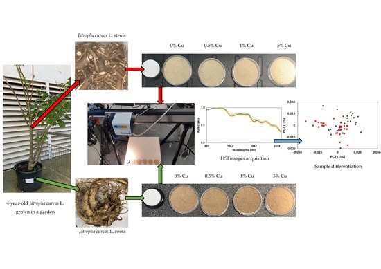
2.1. Raw Material

A Jatropha curcas L. plant that was germinated from seeds sown in vermiculite in a climate chamber, as described elsewhere [3], was transplanted to peat moss in a garden and let grow there. After roughly four years, the 2.2-meter-tall plant was planted in a 50-cm pot and placed in the rooftop of the Faculty of Chemistry of the University of Seville for 90 days to serve as control plant in a phytoremediation research [4]. Afterwards, the plant was cut, separating roots, stems and leaves.

2.2. Metal Content Analysis

Each separate part (root, stem and leaves) was weighed and dried in an oven at 60 °C for approximately 72 h, until constant weight, to remove all moisture. Once all the moisture from the different parts was extracted separately, they were chopped and ground in a hammer mill (Culatti DFH48), and subsequently sieved using a 1-mm mesh. The powder of each sample was stored in Eppendorf tubes until used.

For the analysis of metals, both stems and roots were digested at 220 °C with concentrated HNO₃ in an Ethos One microwave digester (Milestone Srl, Sorisole, Italy). After digestion, the concentrations of Fe, Cr, Cu, Mn, Ni, Pb, Zn, As, Au and Sb were quantified by using a Spectroblue TI ICP-OES (Spectro Analytical Instruments GmbH, Kleve, Germany). The analysis was performed in duplicate and the average metal concentrations are shown in

Table 1. Metal concentrations in Jatropha curcas L. stems and roots.

Sample (mg/kg)	Fe	Cr	Cu	Mn	Ni	Pb	Zn	As	Au	Sb
Stem	35.17	2.99	2.99	9.95	0.83	≤0.4	10.29	≤0.8	≤0.2	≤0.2
RSD	0.57	1.24	5.76	0.22	1.37	-	0.50	-	-	-
Root	261.87	12.20	4.39	13.66	5.86	≤0.2	9.27	≤0.8	≤0.2	≤0.2
RSD	0.59	0.72	8.10	0.41	0.61	-	0.42	-	-	-

RSD: Relative standard deviation.

.

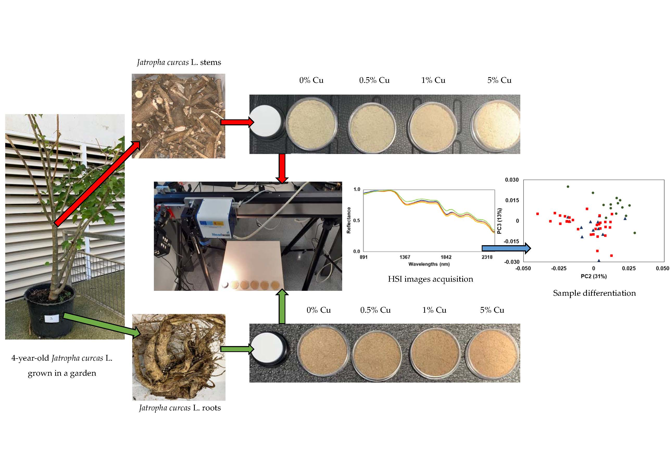
2.3. Sample Preparation and Image Acquisition

Copper was selected because it is the most abundant metal in the mining area of Andalusia (Spain). Fine Cu powder (particle size < 63 µm, purity ≥ 99%) from Merck España (28006 Madrid, Spain) was used for sample preparation. The experimental procedure consisted of preparing four stem samples and four root samples with different known concentrations of copper (0%; 0.5%; 1%; 5% wt.). The dried stems and roots without Cu addition were considered as the samples with 0% wt., since their Cu content was less than 0.0005% wt. (Table 1). Ten samples of each percentage were prepared for stems and roots, totalizing 80 samples. The samples were spread in 3-cm-diameter Petri dishes for image acquisition.

Hyperspectral images were acquired from each image in both sets of experiments in reflectance mode using a SWIR camera (Headwall Photonics SWIR M series, Fitchburg, MA, USA), in the range of 900–2500 nm, with an illuminator of 75 W and a scanning speed of 14.7 mm/s. The program automatically subtracted the white (~99% reflectance) and dark (0% reflectance) references from the acquired images.

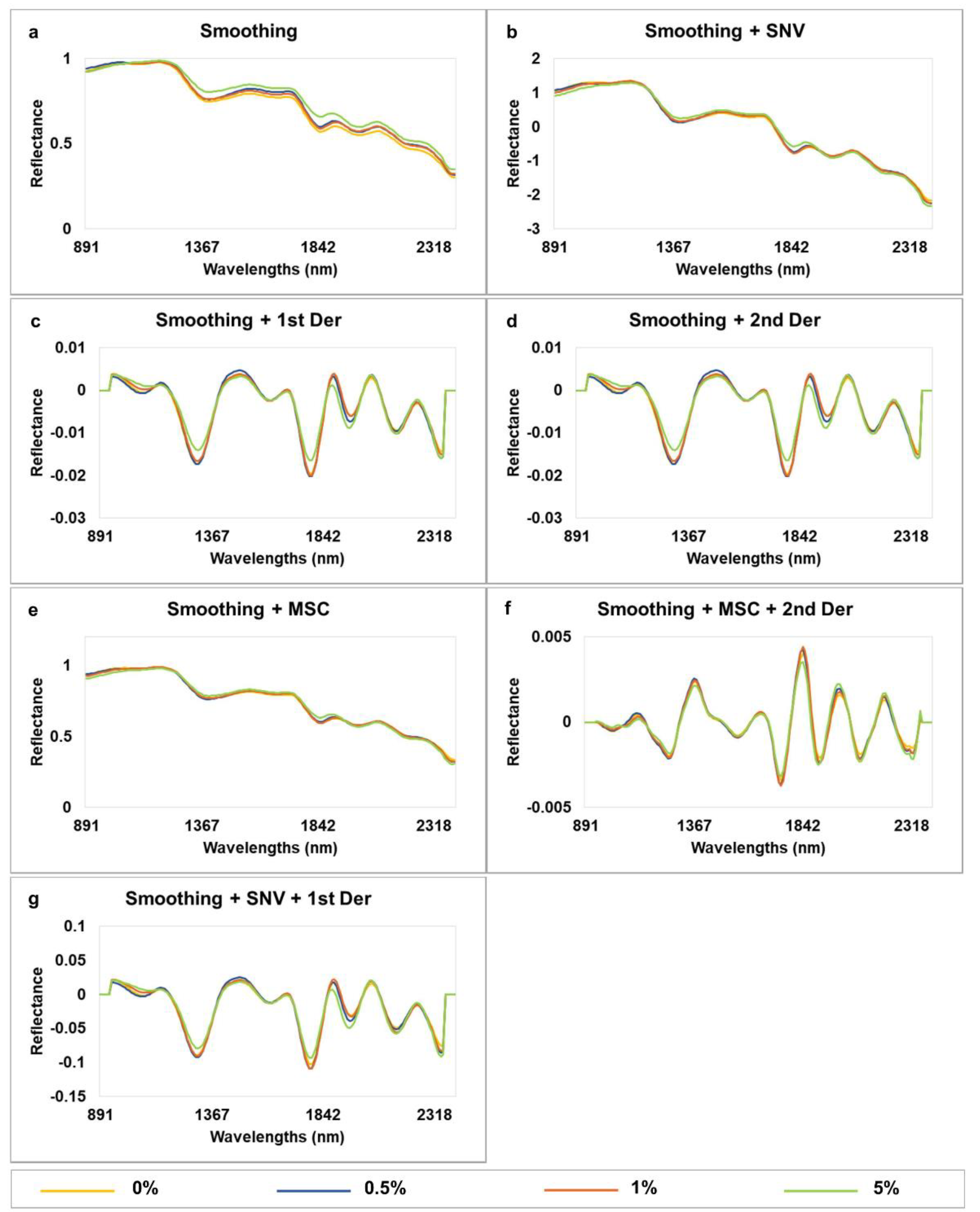
2.4. Spectra Extraction and Multivariate Analysis

Image segmentation and spectrum extraction were performed using a code developed by the research group using the open software Python (version 3.7.0; Python Software Foundation License). The reflectance spectra were normalized, smoothed (Savitzky-Golay) and mean centered before multivariate data analysis. Pre-treatments such as Standard Normal Variate (SNV), Multiplicative Scatter Correction (MSC), first derivative (Savitsky-Golay smoothing, 11 points window, second order polynomial), second derivative (Savitsky-Golay smoothing, 11 points window, second order polynomial) and a combination of MSC + second derivative, and SNV + first derivative, were applied in the dataset to test prior qualitative and quantitative analysis (Principal Component Analysis and Linear Discriminant Analysis). All the multivariate data analysis, including PCA and LDA, was performed using The Unscrambler X 10.4 software (CAMO Software AS, Oslo, Norway).

2.5. Principal Components Analysis (PCA)

Principal Components Analysis was applied to data to have an overview of samples behavior and identify outliers. PCA reduces the information in a large amount of variables to Principal Components (PCs), which are new variables resulted from linear combinations of the original ones [13]. Calibration (70% of the samples) and validation (30% of the samples) sets were selected using PCA scores and Kennard-Stone algorithm. Optimum wavelengths were established manually selecting peaks and valleys in the PCA loadings.

2.6. Linear Discriminant Analysis (LDA)

Linear discriminant analysis (LDA) was performed in all pre-treated data using the optimum wavelengths selected in the loadings plot of PCA. LDA was performed with a leave-one-out cross-validation method and an external validation was carried out with the independent dataset. Models performance was measured in terms of sensitivity, specificity (of validation set) and accuracy of calibration model. Values of sensitivity and selectivity close or equal to 1.00 and accuracy of 100% show good discriminative power.

3. Results and Discussion

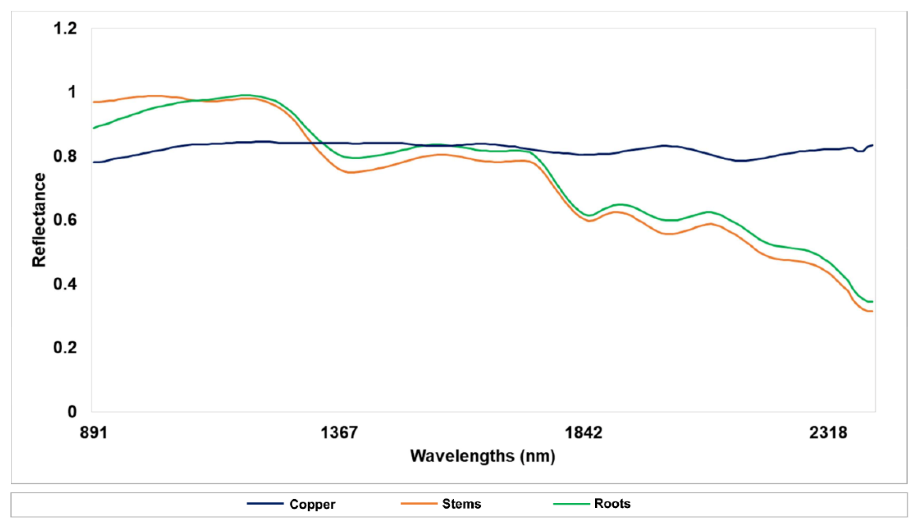
3.1. Spectral Analysis

Spectra of stems and roots with the same percentage of copper were averaged according to the added copper content (Figure 1). The smoothed spectra (Figure 1a) showed very similar shape for all samples, only differing in the intensity of reflectance across the spectral region. Overall, samples with higher amount of copper had higher reflectance. The smoothed spectra and the pre-treated with SNV and MSC were very similar (Figure 1a,b,e, respectively), showing peaks around 1214, 1728, 1918 and 2100 nm, which correspond to stretching vibrations of C-H in the first and second overtone, a stretching vibration of C=O in the second overtone of amides and a combination of O-H deformation and C-O stretching vibration, associated to starch, respectively. The spectra also had a valley at 1306 nm denoting stretching vibration of C-H or a combination of deformation.

The first derivative pre-treatment and a combination of SNV + first derivative spectra (Figure 1c,f) showed peaks and valleys around 1147, 1290, 1414, 1614, 1690, 1956, 2051 and 2166 nm, most attributed to stretching vibrations of C-H or a combination of the first and second overtones, and symmetric and asymmetric modes of N-H group. The intense valley around 1785 nm and the two peaks around 1900 and 2251 nm were also observed in these samples spectra, matching stretching vibrations of C-H in the first overtone in cellulose, stretching vibration of C=O in the second overtone, and a combination of vibrations of O-H stretching and O-H deformation, associated to starch. Moreover, peaks and valleys were noticed around 1100, 1252, 1366, 1566, 1660, 1747, 1842, 1909, 1994, 2089 and 2204 nm for data pre-treated with the second derivative and a combination of MSC + second derivative (Figure 1d,g), most due to stretching vibration of N-H, C-H, S-H and O-H in the first overtone or a combination of deformation [14].

As earlier mentioned, metals, such as copper, do not absorb energy in the near infrared region; therefore, they do not show bands directly associated to them [9]. Figure 2 shows the behavior of smoothed spectra of pure samples, and the difference between NIR spectra of stems and roots and the NIR spectrum of pure copper is clear. Notwithstanding, the indirect determination of inorganic Cu is possible, as demonstrated in the following sections, probably due to the balance between organic and inorganic components. This was the main objective of the current study. However, future studies should investigate the influence of chromogenic ligands and fluorescence probes, iron oxides, clay minerals and organic matter, present in plants, and how they might affect the identification of the components by optical methods.

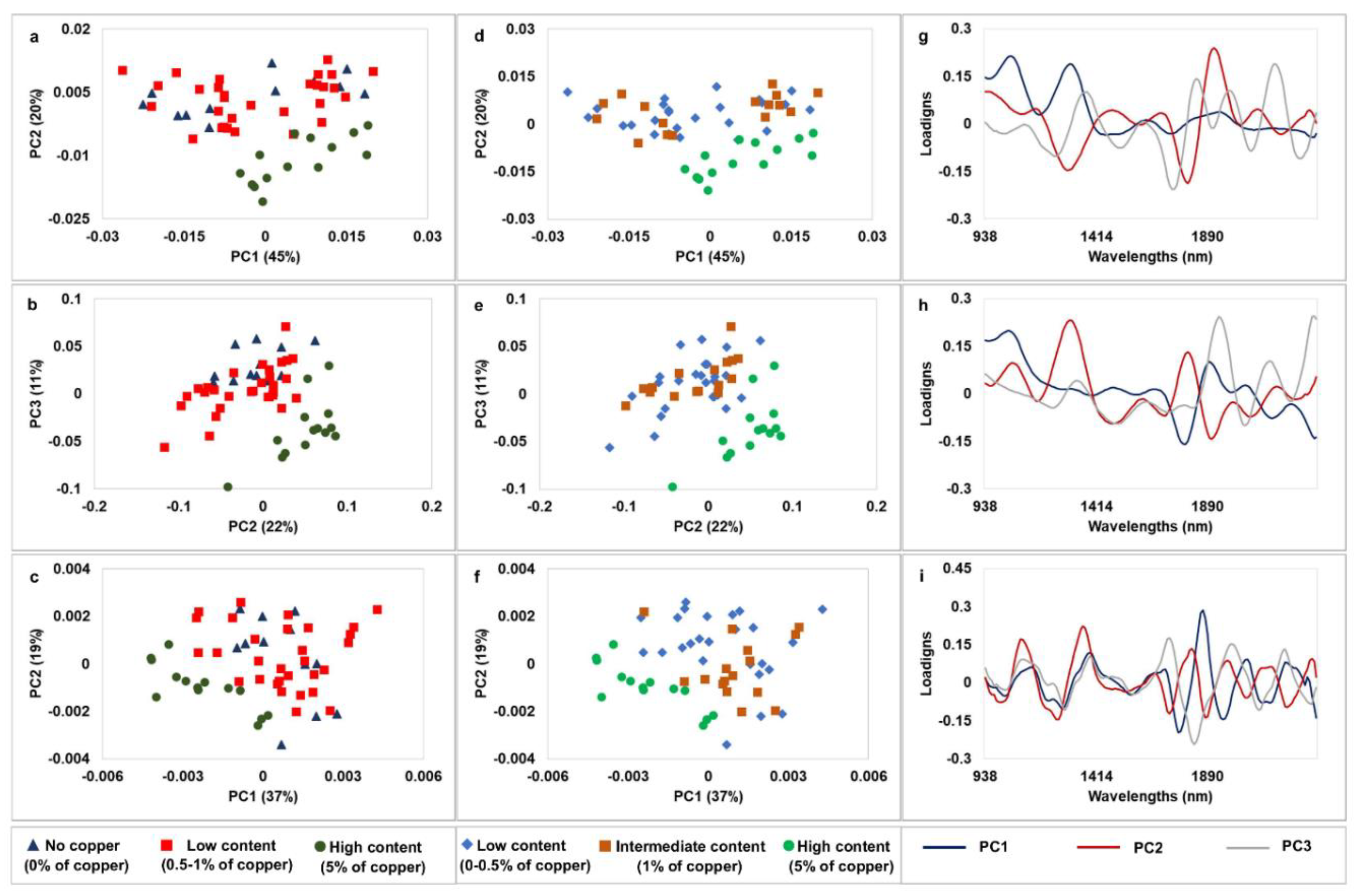
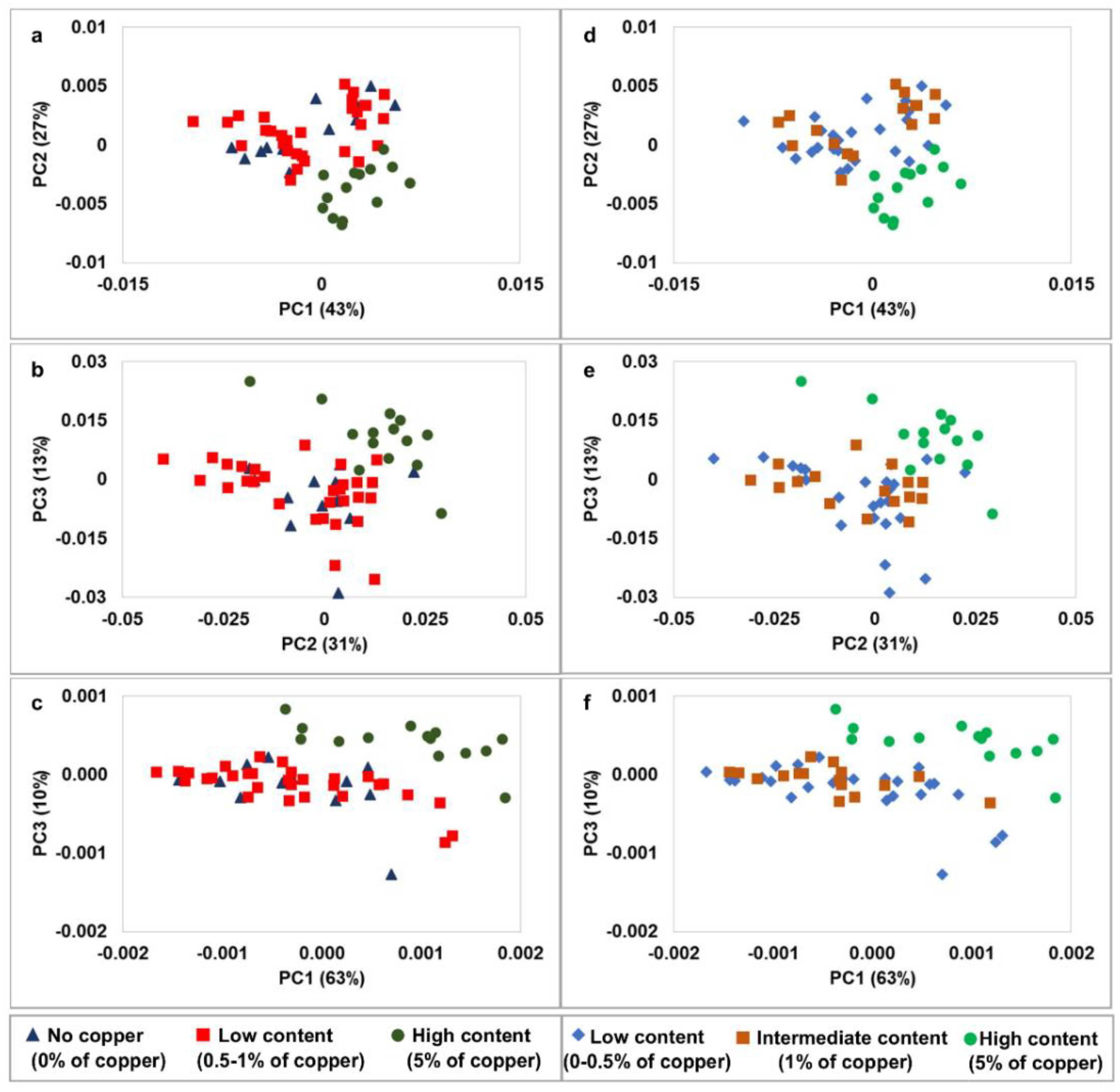
3.2. Principal Components Analysis (PCA)

Considering the concept of pairwise classifications, samples of stems and roots added of copper were evaluated in three strategies: 1—Four classes: Class 1–0% copper, Class 2–1% copper, Class 3–0.5% copper and Class 4–5% copper; 2—Three classes: Class 1—“No copper” (0% of copper), Class 2—“Low content” (0.5–1% of copper) and Class 3—“High content” (5% of copper); and 3—Three classes: Class 1—“Low content” (0–0.5% of copper), Class 2—“Intermediate content” (1% of copper) and Class 3—“High content” (5% of copper). PCA was performed in spectra data with all pre-treatments and the outcome was evaluated in terms of the three groups of classes. Figure 3 describes the PCA scores and loadings of samples data. The pre-treatments that better succeeded in separating samples according to their groups were the first derivative, a combination of SNV + first derivative and the second derivative (Figure 3a–c, respectively).

Figure 3a,d show the score plots after 1st derivate pre-treatment, considering strategies 2 and 3, respectively. PC1 and PC2 explained 65% of the total variance among samples in both cases. In strategy 2, samples with “No copper” and “Low content” showed some overlap, whereas samples with “High content” were grouped in a separate cluster in the right part of PC1 and negative side of PC2. In strategy 3, samples with “Low content” and “Intermediate” also had some overlap, whereas samples with “High content” were grouped in a separate cluster in the right part of PC1 and negative side of PC2.

Figure 3b,e displays PC2 and PC3 of data pre-treated with SNV + first derivative combined, showing similar behavior. That means, overlapping of Classes 1 and 2 and a separate cluster in the right part of PC1 and negative side of PC2 with samples belonging to Class 3. Figure 3c,f show that data with the second derivative had 56% of the total variance explained by PC1 and PC2. In this case, samples of Class 3 are displayed in the negative part of PC and PC3, while samples of Classes 1 and 2 are disperse in the positive side.

Figure 3g–i show the loadings plot of PC1, PC2 and PC3. The peaks and valleys on these plots were selected as optimum wavelengths and a new PCA was calculated with these reduced spectra (Figure 4). Except for the second derivative PCA, which now displays samples belonging to Class 3 in the positive side of PC1 and PC3, the recalculated PCA with the two other pre-treatments had similar behavior as with full spectra. However, variable selection seems to have reduced the dispersibility among those samples belonging to the same classes. Then, these wavelengths were used as input for the development of LDA models. Selecting few wavelengths helps reducing the number of predictors and sometimes reduces noise, thus providing better separation among samples for classification models [6,15].

3.3. Linear Discriminant Analysis (LDA)

Table 2. Models performance of LDA for qualitative analysis of copper in stems and roots.

STRATEGY 1: C1—0% Copper, C2—1% Copper, C3—0.5% Copper, and C4—5% Copper
Pre-Treatment	Wavelengths	Sensitivity (Validation)				Specificity (Validation)				Accuracy—Calibration Model (%)
		C1	C2	C3	C4	C1	C2	C3	C4
Smoothing	1271, 1376, 1737, 1899, 2013, 2089	0.38	0.67	0.14	1.00	0.88	0.71	0.76	1.00	69.64
Smoothing + SNV	1147, 1376, 1737, 1851, 1928, 2013, 2118, 2223	0.38	0.67	0.43	0.83	0.69	0.86	0.82	1.00	76.79
Smoothing + first Derivative	1042, 1166, 1309, 1366, 1480, 1709, 1747, 1813, 1918, 1975, 2061, 2185	0.50	0.67	0.14	1.00	0.94	0.67	0.82	1.00	85.71
Smoothing + second Derivative	1138, 1271, 1376, 1556, 1709, 1775, 1871, 1947, 2051, 2137, 2232	0.38	0.33	0.14	1.00	0.69	0.86	0.71	1.00	75.00
Smoothing + MSC	1147, 1376, 1699, 1861, 2013, 2223	0.38	0.67	0.43	0.83	0.81	0.76	0.82	1.00	69.64
Smoothing + MSC + second Derivative	1081, 1271, 1376, 1556, 1633, 1756, 1851, 1947, 2032, 2108, 2213	0.25	0.33	0.43	0.67	0.75	0.67	0.82	1.00	71.43
Smoothing + SNV + first Derivative	1042, 1166, 1309, 1480, 1671, 1747, 1899, 2061, 2166	0.50	0.67	0.00	0.83	0.88	0.62	0.82	1.00	85.71
STRATEGY 2: C1—“No Copper” (0%), C2—“Low Content” (0.5-1%) and C3—“High Content” (5%)
Pre-Treatment	Wavelengths	Sensitivity (Validation)				Specificity (Validation)				Accuracy—Calibration Model (%)
		C1	C2		C3	C1	C2		C3
Smoothing	1271, 1376, 1737, 1899, 2013, 2089	0.63	0.70		1.00	0.81	0.79		1.00	78.57
Smoothing + SNV	1147, 1376, 1737, 1851, 1928, 2013, 2118, 2223	0.63	0.40		0.83	0.56	0.79		1.00	76.79
Smoothing + first Derivative	1042, 1166, 1309, 1366, 1480, 1709, 1747, 1813, 1918, 1975, 2061, 2185	0.63	0.70		1.00	0.81	0.79		1.00	85.71
Smoothing + second Derivative	1138, 1271, 1376, 1556, 1709, 1775, 1871, 1947, 2051, 2137, 2232	0.75	0.40		1.00	0.63	0.86		1.00	83.93
Smoothing + MSC	1147, 1376, 1699, 1861, 2013, 2223	0.50	0.50		0.83	0.63	0.71		1.00	76.79
Smoothing + MSC + second Derivative	1081, 1271, 1376, 1556, 1633, 1756, 1851, 1947, 2032, 2108, 2213	0.50	0.50		0.67	0.63	0.64		1.00	82.14
Smoothing + SNV + first Derivative	1042, 1166, 1309, 1480, 1671, 1747, 1899, 2061, 2166	0.75	0.70		1.00	0.81	0.86		1.00	83.93
STRATEGY 3: C1—“Low Content” (0–0.5%), C2—“Intermediate Content” (1%) and C3—“High Content” (5%)
Pre-Treatment	Wavelengths	Sensitivity (Validation)				Specificity (Validation)				Accuracy—Calibration Model (%)
		C1	C2		C3	C1	C2		C3
Smoothing	1271, 1376, 1737, 1899, 2013, 2089	0.33	0.33		1.00	0.78	0.52		1.00	69.64
Smoothing + SNV	1147, 1376, 1737, 1851, 1928, 2013, 2118, 2223	0.67	0.67		0.83	0.78	0.76		1.00	78.57
Smoothing + first Derivative	1042, 1166, 1309, 1366, 1480, 1709, 1747, 1813, 1918, 1975, 2061, 2185	0.40	1.00		1.00	1.00	0.57		1.00	82.14
Smoothing + second Derivative	1138, 1271, 1376, 1556, 1709, 1775, 1871, 1947, 2051, 2137, 2232	0.67	0.67		1.00	0.89	0.76		1.00	78.57
Smoothing + MSC	1147, 1376, 1699, 1861, 2013, 2223	0.40	0.67		0.83	0.78	0.57		1.00	75.00
Smoothing + MSC + second Derivative	1081, 1271, 1376, 1556, 1633, 1756, 1851, 1947, 2032, 2108, 2213	0.53	0.33		0.67	0.78	0.57		1.00	80.36
Smoothing + SNV + first Derivative	1042, 1166, 1309, 1480, 1671, 1747, 1899, 2061, 2166	0.47	0.67		1.00	0.89	0.62		1.00	85.71

shows the models performance of LDA models for qualitative analysis of copper in stems and roots. The classifications were based in the three strategies mentioned in PCA analysis. As in PCA of the first strategy (data not shown), the results were not suitable. Even though some of the calibration models have shown good accuracy, the prediction ability for some of the classes was very low, with values of sensitivity close or equal to 0. On the other hand, the second strategy provided good accuracy for all the calibration models, ranging from 76.79–85.71%. In general, the values of sensitivity and specificity were above 0.40 and 0.56, respectively. The first derivative had the best accuracy for the calibration model (85.71%), followed by the second derivative and a combination of SNV + first derivative (83.93%). However, this last had the highest values of sensitivity and specificity (>0.70) in the external validation. Therefore, this was considered the best model for this strategy of classification, since it showed good results for all three parameters at the same time.

Values of sensitivity and specificity for validation models above 0.8 are adequate for classification models with screening purposes. For instance, values of 0.8 or higher in the identification of different types of barley have been achieved [7]. Depending on the composition of samples analyzed and the type of feature to be identified, classification models may range between different levels of sensitivity, specificity, accuracy or other figures of merit used to assess models performance [16]. This approach could be used for screening purposes, identifying heavy-metal contaminated plants that could be subsequent used in different industrial processes [17].

The LDA models accuracy considering the third strategy achieved acceptable results, ranging from 69.64% to 85.71%. The model developed with SNV + first derivative had the best model accuracy (85.71%), followed by the first derivative (82.14%), and a combination of MSC + second derivative (80.36%). However, at least one class in each classification had values of sensitivity lower than 0.50. Although the accuracy of the second derivative and SNV models (78.57%) was lower than the first three, the ability to predict the samples into their classes was better in these models. The values of sensitivity and specificity were above 0.67 and 0.76, respectively. The proposed approach demonstrated feasibility to differentiate samples with different amounts of added copper by NIR-HSI. Further studies should consider the interference of other components in the sample, and how they could affect the spectral information in the near-infrared range.

4. Conclusions

Despite the inherent difficulty of quantify the concentration of metals such as Cu by their NIR absorbance, the results illustrate that NIR-HSI can differentiate plants (roots or stems) samples with different Cu concentrations.

From the PCA plots, it could be observed that, among the spectral pre-treatments assayed, those that better succeeded in separating samples according to their groups were the first derivative, a combination of SNV + first derivative and the second derivative. Samples from classes 1 and 2 had more misclassified samples while the results of the sensitivity and specificity in class 3 were always close or equal to one.

Based on LDA results, the second strategy was considered the most suitable for differentiate stem and root samples with different Cu concentrations. This strategy achieved good accuracy (76.79–85.71%) for all the calibration models, where the first derivative was the spectral pre-treatment that provided the best accuracy. Notwithstanding, the second derivative and a combination of SNV + first derivative showed the highest values of sensitivity and specificity (>0.70) in the external validation along with a good accuracy in the calibration model (83.93%).

Further research on the determination of other highly contaminating heavy metals by NIR-HSI are required to prove that this technology can be used for the in situ determination of the actual level of metals in plants over phytoremediation period. Moreover, the potential interferences due to the presence of chromogenic ligands and fluorescence probes, iron oxides, clay minerals and organic matter should be investigated.

References

1. Jiménez-Moraza, C.; Iglesias, N.; Palencia, I. Application of sugar foam to a pyrite-contaminated soil. Miner. Eng. 2006, 19, 399–406. [Google Scholar] [CrossRef]
2. Shi, T.; Chen, Y.; Liu, Y.; Wu, G. Visible and near-infrared reflectance spectroscopy-An alternative for monitoring soil contamination by heavy metals. J. Hazard. Mater. 2014, 265, 166–176. [Google Scholar] [CrossRef] [PubMed]
3. Álvarez-Mateos, P.; Alés-Álvarez, F.J.; García-Martín, J.F. Phytoremediation of highly contaminated mining soils by Jatropha curcas L. and production of catalytic carbons from the generated biomass. J. Environ. Manag. 2019, 231, 886–895. [Google Scholar] [CrossRef] [PubMed]
4. García Martín, J.F.; del González Caro, M.C.; del López Barrera, M.C.; Torres García, M.; Barbin, D.; Álvarez-Mateos, P. Metal accumulation by Jatropha curcas L. adult plants grown on heavy metal-contaminated soil. Plants 2020, 9, 418. [Google Scholar] [CrossRef] [PubMed] [Green Version]
5. Badaró, A.T.; Garcia-Martin, J.F.; del López-Barrera, M.C.; Barbin, D.F.; Alvarez-Mateos, P. Determination of pectin content in orange peels by near infrared hyperspectral imaging. Food Chem. 2020, 323, 126861. [Google Scholar] [CrossRef] [PubMed]
6. García Martín, J.F. Optical path length and wavelength selection using Vis/NIR spectroscopy for olive oil’s free acidity determination. Int. J. Food Sci. Technol. 2015, 50, 1461–1467. [Google Scholar] [CrossRef] [Green Version]
7. Lopes, J.F.; Ludwig, L.; Barbin, D.F.; Grossmann, M.V.E.; Barbon, S. Computer vision classification of barley flour based on spatial pyramid partition ensemble. Sensors 2019, 19, 2953. [Google Scholar] [CrossRef] [PubMed] [Green Version]
8. Chandrasekaran, I.; Panigrahi, S.S.; Ravikanth, L.; Singh, C.B. Potential of near-infrared (NIR) spectroscopy and hyperspectral imaging for quality and safety assessment of fruits: An overview. Food Anal. Methods 2019, 12, 2438–2458. [Google Scholar] [CrossRef]
9. Moros, J.; De Vallejuelo, S.F.O.; Gredilla, A.; De Diego, A.; Madariaga, J.M.; Garrigues, S.; De La Guardia, M. Use of reflectance infrared spectroscopy for monitoring the metal content of the estuarine sediments of the Nerbioi-Ibaizabal River (Metropolitan Bilbao, Bay of Biscay, Basque Country). Environ. Sci. Technol. 2009, 43, 9314–9320. [Google Scholar] [CrossRef] [PubMed]
10. Wu, Y.; Chen, J.; Ji, J.; Gong, P.; Liao, Q.; Tian, Q.; Ma, H. A Mechanism study of reflectance spectroscopy for investigating heavy metals in soils. Soil Sci. Soc. Am. J. 2007, 71, 918–926. [Google Scholar] [CrossRef]
11. Rathod, P.H.; Rossiter, D.G.; Noomen, M.F.; van der Meer, F.D. Proximal spectral sensing to monitor phytoremediation of metal-contaminated soils. Int. J. Phytoremediat. 2013, 15, 405–426. [Google Scholar] [CrossRef] [PubMed]
12. Manios, T.; Stentiford, E.I.; Millner, P.A. The effect of heavy metals accumulation on the chlorophyll concentration of Typha latifolia plants, growing in a substrate containing sewage sludge compost and watered with metaliferus water. Ecol. Eng. 2003, 20, 65–74. [Google Scholar] [CrossRef]
13. Verdú, S.; Vásquez, F.; Ivorra, E.; Sánchez, A.J.; Barat, J.M.; Grau, R. Hyperspectral image control of the heat-treatment process of oat flour to model composite bread properties. J. Food Eng. 2017, 192, 45–52. [Google Scholar] [CrossRef]
14. Osborn, B.G.; Fearn, T.; Hindle, P.H. Theory of near infrared spectroscopy. In Practical NIR Spectroscopy with Applications in Food and Beverage Analysis; Longman Singapore Publishiers (Pte) Ltd.: London, UK, 1993; pp. 13–35. [Google Scholar]
15. Barbin, D.F.; Badaró, A.T.; Honorato, D.C.B.; Ida, E.Y.; Shimokomaki, M. Identification of Turkey meat and processed products using near infrared spectroscopy. Food Control 2020, 107, 106816. [Google Scholar] [CrossRef]
16. Nolasco-Perez, I.M.; Rocco, L.A.C.M.; Cruz-Tirado, J.P.; Pollonio, M.A.R.; Barbon, S.; Barbon, A.P.A.C.; Barbin, D.F. Comparison of rapid techniques for classification of ground meat. Biosyst. Eng. 2019, 183, 151–159. [Google Scholar] [CrossRef]
17. García-Martín, J.F.; Alés-Álvarez, F.J.; Torres-García, M.; Feng, C.-H.H.; Álvarez-Mateos, P. Production of oxygenated fuel additives from residual glycerine using biocatalysts obtained from heavy-metal-contaminated Jatropha curcas L. roots. Energies 2019, 12, 740. [Google Scholar] [CrossRef] [Green Version]
Figure 1. Spectra of stems and roots and copper pre-treated with: (a) Smoothing, (b) Smoothing + Standard Normal Variate (SNV), (c) Smoothing + first derivative, (d) Smoothing + second derivative, (e) Smoothing + Multiplicative Scatter Correction (MSC), (f) Smoothing + MSC + second derivative, (g) Smoothing + SNV + first derivative.
Processes 08 00823 g001
Figure 2. Smoothed spectra of pure samples: Copper (blue), Stems (orange) and Roots (green).
Processes 08 00823 g002
Figure 3. PCA scores and loadings of stems and roots and copper pre-treated with: (a,d,g) Smoothing + first derivative, (b,e,h) Smoothing + SNV + first derivative, (c,f,i) Smoothing + second derivative.
Processes 08 00823 g003
Figure 4. PCA scores of stems and roots and copper after variable selection pre-treated with: (a,d) Smoothing + first derivative, (b,e) Smoothing + SNV + first derivative, (c,f) Smoothing + second derivative.
Processes 08 00823 g004