Potential Dynamics of CO2 Stream Composition and Mass Flow Rates in CCS Clusters

1
Institute of Energy Systems (IET), Hamburg University of Technology, Denickestr. 15, D-21073 Hamburg, Germany
2
DBI Gas-und Umwelttechnik GmbH, Karl-Heine-Str. 109/111, D-04229 Leipzig, Germany
3
Federal Institute for Geosciences and Natural Resources (BGR), Stilleweg 2, D-30655 Hannover, Germany
*
Author to whom correspondence should be addressed.
Processes 2020, 8(9), 1188; https://0-doi-org.brum.beds.ac.uk/10.3390/pr8091188
Submission received: 27 July 2020
/
Revised: 9 September 2020
/
Accepted: 11 September 2020
/
Published: 18 September 2020
(This article belongs to the Special Issue Carbon Capture, Utilization and Storage Technology)
Abstract
:Temporal variations in CO2 stream composition and mass flow rates may occur in a CO2 transport network, as well as further downstream when CO2 streams of different compositions and temporally variable mass flow rates are fed in. To assess the potential impacts of such variations on CO2 transport, injection, and storage, their characteristics must be known. We investigated variation characteristics in a scenario of a regional CO2 emitter cluster of seven fossil-fired power plants and four industrial plants that feed captured CO2 streams into a pipeline network. Variations of CO2 stream composition and mass flow rates in the pipelines were simulated using a network analysis tool. In addition, the potential effects of changes in the energy mix on resulting mass flow rates and CO2 stream compositions were investigated for two energy mix scenarios that consider higher shares of renewable energy sources or a replacement of lignite by hard coal and natural gas. While resulting maximum mass flow rates in the trunk line were similar in all considered scenarios, minimum flow rates and pipeline capacity utilisation differed substantially between them. Variations in CO2 stream composition followed the power plants’ operational load patterns resulting e.g., in stronger composition variations in case of higher renewable energy production.
1. Introduction
Capturing CO2 at large stationary point sources such as industrial plants or power stations and storing it in deep geological formations (so-called CCS technology) is one technological option to reduce anthropogenic CO2 emissions (e.g., [1,2,3]). Captured CO2 may also be utilised as a raw material for the production of basic chemicals and precursors for e.g., fuels or polymers for an envisaged circular economy (e.g., [4,5]). Captured CO2 will not be 100% pure CO2, but may contain other substances (“impurities”) depending on the source process, the capture technology, and the implementation of further purification steps. In the following, the term “CO2 streams” is used for streams from CO2 capture processes that consist of CO2 and impurities (cf. [6,7]).
Transporting CO2 streams by setting up a regional pipeline collection network and using a trunk line for long-distance transport to the storage or utilisation site may help to minimise the overall cost of the transport system (e.g., [1,2]). According to Directive 2009/31/EC [6], CO2 transport pipelines “should be designed so as to facilitate access of CO2 streams meeting reasonable minimum composition thresholds”. It is not yet known how such composition thresholds may be defined and which CO2 qualities may be viable in practical application when CO2 streams with larger quantities and various types of impurities are also considered. The CO2 pipelines that are currently in operation mostly transport high purity CO2 containing, if at all, small amounts of impurities with reducing properties (e.g., [8]).
To define minimum composition thresholds in CO2 transport networks, the impacts of different impurities on CO2 transport, injection, and storage must be known. Impurities may affect (i) thermophysical properties of CO2 streams with various implications for transport, injection, and geological storage (e.g., [9,10,11]) and (ii) the reactivity of the CO2 stream with implications for the corrosion behaviour of e.g., pipeline material and plant components (e.g., [12]), as well as for geotechnically relevant rock properties (e.g., [13]). When CO2 streams from different sources and with different compositions are fed into a pipeline network, this will result in a temporal variation of both mass flow rates and CO2 stream compositions in the network, if streams are fed in with varying rates. These temporal compositional variations will result in variations of the chemical reactivity and the thermophysical properties of the combined CO2 streams. In turn, these variations may affect CO2 transport, injection, and storage in other ways than CO2 streams of constant composition. Likewise, variations in mass flow rates may require an adaptation of pipeline design and design parameters. As a basis for assessing impacts of CO2 streams with varying compositions and mass flow rates on CCS systems, their variation characteristics in such systems must be known.
The technical and economic feasibility of a flexible operation of fossil-fired power plants equipped with CO2 capture has been assessed in several studies and plant operating profiles have been modelled for specific future energy system scenarios with intermittent power generation from renewable energy sources (e.g., [14,15]). Focussing on flexible power generation, few studies have assessed the resulting variations in mass flow rates and their implications on CO2 transport and storage systems (e.g., [16,17,18,19]). To our knowledge, the associated variability of CO2 stream composition due to mixing of CO2 streams in larger pipeline networks has not been investigated so far. In addition, the role of industrial plants and their operational profiles for mass flow rates and CO2 stream composition in CO2 transport networks has not yet been addressed.
To fill this gap, variations of CO2 stream composition and mass flow rates in a generic pipeline network as a part of a CCS cluster system were simulated in this study using an in-house developed network analysis tool [20]. This work is based on a scenario of a CCS cluster system, i.e., a regional cluster of different CO2 emitters (industrial plants and power stations) from which captured CO2 streams are collected in a regional pipeline network and jointly transported (in a trunk line) to an injection site. Hourly averages of mass flow rates fed in by each plant were derived from real power production data in Germany at the start of the study in 2015 and from typical annual operational loads of respective industrial plants. Variations in mass flow rates and CO2 stream compositions were also simulated for two additional scenarios reflecting possible future changes in the energy mix to allow for an efficient pipeline design considering the pipeline’s entire lifetime.
This work was conducted as part of the collaborative project CLUSTER [21].
2. Materials and Methods
2.1. Selection and Modelling of CO2 Emitters
2.1.1. Selection of CO2 Emitters
In Germany, the energy sector and industrial plants are collectively responsible for about 60% of the national total greenhouse gas emissions [22]. Within these two sectors, the large stationary plants are particularly suitable for CO2 capture, both in technical and economical terms. For this study, a model plant park (or model cluster) consisting of four industrial plants and seven power plants was defined (Table 1) reflecting the ratio of CO2 emissions of the energy and the industry sector in Germany at the beginning of the study in 2015. Furthermore, the share of different fossil fuels in Germany’s power production was considered for plant definition. Industrial plants were chosen from industries with highest annual CO2 emissions (as of 2015). One of the three technology paths for CO2 capture that are currently under development was assigned to each plant:
- Post-Combustion Capture: In this study: CO2 capture from flue gas by absorption with monoethanolamine (MEA).
- Oxyfuel: Production of a CO2-rich flue gas flow through removal of N2 from the air used for combustion.
- Pre-Combustion Capture: In this study: CO2 capture from the synthesis gas of a coal gasification.
All these technology paths currently appear promising, each showing specific advantages and disadvantages. Absorption by amine solutions is currently the most mature and thus the most widely used technology, e.g., [4].
2.1.2. Composition of CO2 Streams Captured at the Individual CO2 Emitters
Depending on the applied capture technology, there are different types and amounts of impurities in the captured CO2 streams. Literature data collated in [23] was used to define CO2 stream compositions of the different plants and capture facilities (Table 2). The compositions of all CO2 streams captured with the same capture technology were assumed to be equal, with the exception of cement plants: As the used fuel does not contain sulfur, there is also no SOx in the generated CO2 stream. Instead, there is a proportionally greater proportion of the remaining impurities listed for the other post-combustion capture (PCC) plants (data not included in Table 2). The H2O concentration of captured CO2 streams was limited to 50 ppmv in the scenarios following [23,24]. Each emitter’s CO2 stream composition was assumed to be constant over time.
2.1.3. Modelling of CO2 Emitters
For modelling of varying CO2 mass flow rates and CO2 stream compositions in the whole CCS chain, mass flow rates of CO2 streams captured from the power and industrial plants were determined. For this, each of the seven power plants and the four industrial plants was defined in terms of plant size (Table 1), dynamic behaviour, and composition of the captured CO2 stream (Table 2). Conventional power plant processes were modelled using the software packages EBSILON®Professional, AspenPlus® and Matlab® based on characteristics of currently operating plants in Germany that are in line with the current state of technology. For modelling the capture of CO2 from flue gases, conventional power plants were adapted to the modified process management and boundary conditions.
The modelling of the power plants’ dynamic behaviour was conducted on the basis of the actual electricity production in Germany in the year 2015 based on data from the ENTSO-E Transparency Platform [25] as well as market data on actual electricity generation provided by the European Energy Exchange AG [26]. In the latter data, the power output is divided into different generating technologies and is given in quarter-hour increments. A shift plan for the regarded power plants was created based on these data. Deployment of the individual power plants was carried out in accordance with the merit order, i.e., plants with the lowest electricity generation costs were deployed first to meet the electricity demand. Additionally, a priority feed-in for electricity from renewable energy sources was considered. Hence, the power production from fossil-fired power plants was adapted to both the variable renewable power generation and the variable electricity demand.
Furthermore, power plant specific data for full and part load, down time for maintenance, an acceptable load change gradient, and a specific minimum load of each power plant were defined for modelling following [27,28,29,30]. An unrealistic power plant mode of operation with frequent start-ups and shutdowns was avoided in the modelling by the definition of a minimum downtime, a minimum runtime per start-up, and maximum load change gradients. For example, for the lignite-fired power plant with post-combustion capture (Lignite PCC), a minimum downtime of 8 h, a minimum runtime of 6 h, and maximum load change gradients of 2% and 5% for load increase and decrease, respectively, were defined. As one boundary condition in the power plants’ modelling, a thermal input of 1220 MW was used. In addition, a CO2 capture rate of 90% as well as a compression of the CO2 stream to a pressure of 11 MPa and cooling to a temperature of 313 K were considered. Only the Integrated Gasification Combined Cycle (IGCC) power plant with CO2 capture technology (short: PreCC) was defined with a thermal input of 900 MW and a CO2 capture rate of 85%.
Modelling of the industrial processes steel production, cement production, and oil refining was based on plants of typical sizes in Germany. The basic data for the regarded industrial plants were obtained from the Best Available Technology (BAT) data sheets [31,32,33]. CO2 capture plants developed for power plants were adapted to the conventional industrial processes. In particular, the higher CO2 partial pressure in the industrial process gases as compared to power plant flue gases was taken into account for the capture plant design. The process gas composition of each plant with respect to CO2 and the most abundant impurities N2, Ar, O2 as well as H2O were considered for the determination of the energy demand of CO2 capture in each case. This included the reduction of the H2O concentration in the CO2 stream to a final value of 50 ppmv (cf. Table 2).
In the presentation of the results, the term “pipeline mass flow rate” is used whenever a mass flow rate of an impure CO2 stream is referred to.
2.1.4. Development of Energy Mix Scenarios
On the basis of the defined electricity demand and by taking into account the plant-specific key figures of all considered power plants and industrial plants, three different energy mix scenarios were modelled in line with emission reduction measures given in the Government’s Climate Action Programme 2050 [34]. The baseline scenario reflects the conditions in Germany in 2015 with a share of renewable energy of 27% [35]. For the scenario “RE 45%”, an expansion of renewable energies to a share of 45% of the total electricity production was taken into account. For modelling this scenario, the total electricity demand as well as the wind and solar conditions of the baseline scenario were used. In the scenario “No lignite”, a fuel shift was assumed, so that the lignite-fired power plants are replaced by two additional coal-fired power plants and another gas-fired power plant. Apart from this, no other changes were made in comparison to the baseline scenario, i.e., the share of energy from renewable sources is also 27%.
2.2. Transport Network and CO2 Stream Properties
2.2.1. Spatial Array
The CO2 transport network in the scenario is composed of two parts: (i) a regional network that collects CO2 streams of the 11 CO2 emitters and (ii) a single trunk pipeline that connects the regional cluster with the fictive injection and storage site located offshore. The spatial array of all CO2 emitters in the regional cluster was defined according to actual locations of similar industrial plants in Germany (Figure 1). The regional cluster covers an area of 75 km in diameter.
The collection network was set up so that CO2 streams are collected in a regional network with an as short as possible overall pipeline length. As a result, the selected collection network contains conduits of an overall length of 160.5 km. The lengths of individual pipeline segments range from 4.6 km (segment 10; Figure 1) to 22 km (segment 6; Figure 1). Each “connecting segment” (1, 4, 5, 7, 11, 12, 13, 14, 15, 16) connects one plant to the collection network. CO2 streams are then transported by “interconnecting segments” (3, 9, 10) to “collecting segments” (2, 6, 8) and further to the trunk line. The trunk line has a length of 300 km and 100 km in its onshore and offshore parts, respectively.
2.2.2. Network Analysis Tool
For calculating the dynamics of CO2 stream composition and mass flow rates in pipeline networks and the resulting thermophysical fluid properties, a network analysis tool was developed [20]. The algorithm underlying the network analysis tool is based on a tool published earlier [36]. The earlier calculation tool for single pipelines was transferred into the software package Matlab® and adopted for the calculation of CO2 stream compositions and mass flow rates in complex pipeline networks. The Matlab® algorithm calculates pipeline mass flow rates and CO2 stream compositions in each pipeline segment (hourly values) based on the CO2 production and feed-in characteristics of each CO2 emitter (as hourly averages throughout one year) and pre-calculated pipeline dimensions. For example, inner diameters of the trunk line were pre-calculated as 68 cm for the scenarios “RE 27%” and “RE 45%” and as 63 cm for the scenario “No lignite”. In addition, the pressure distribution within the network is calculated for each hourly interval following the reverse flow direction from the trunk line to the CO2 emitters. In addition, the algorithm calculates thermophysical properties as a function of CO2 stream composition using a Matlab® implementation of the programme REFPROP that routinely calculates mixture properties by a model applying mixing rules to the Helmholtz energy of the mixture components and using a departure function to account for non-ideal mixing [37]. Further, the flow velocity is calculated as a function of pipeline mass flow rates, surface roughness of the pipeline material, inner diameter of the pipe, viscosity, and density of the CO2 stream (as a function of its composition and the pressure and temperature conditions in the respective pipeline segment). All calculations are executed iteratively until the following conditions are met: (i) the calculated pressure at the end of the trunk line must be above the determined minimum pressure (as a function of stream composition; see below), (ii) the flow velocity within the pipeline sections must not exceed a value of 3 m/s to avoid pipe erosion (cf. [38]).
In the scenarios, CO2 transport in the regional cluster is accomplished without intermediate pumping stations within the collection network; booster stations are not planned before the trunk line entry. In consequence, the entry to the trunk line is the point with the lowest pressure in the regional collection network. Thus, the pressure at the entry of each pipeline segment must be sufficiently high to maintain pressure above the minimum pressure while compensating for pressure losses during transport within this segment. The minimum pressure was defined as the pressure to be maintained in order to transport the CO2 stream in single phase.
As a simplification, for each pipeline segment, a constant ground temperature of 288 K was assumed, and the transported CO2 stream was assumed to be at thermodynamic equilibrium with its surrounding, as the pipeline network is not insulated. Thus, the CO2 stream is transported as a dense-phase fluid. Chemical reactions between different impurities within the CO2 streams, in particular at mixing, were not considered following [39].
3. Results
3.1. CO2 Emitters
3.1.1. Characteristics of Power Plants and Industrial Plants
Modelled net efficiency curves of the power plants with CO2 capture are depicted in Figure 2 as a function of the relative thermal input. For PCC power plants, the optimum operating point in terms of thermal heat demand for a regeneration of the solvent (monoethanolamine, MEA), i.e., the optimal solvent circulation rate of each PCC plant, was chosen. Regarding the oxyfuel power plants, a less steady course of the net efficiency curve is apparent (Figure 2) as one or two compressor trains may be deactivated at 75% and 50% load, respectively, in case of an installation of a four-part flue gas compressor, which results in a significant reduction of power consumption. Due to the numerous links between the single plant components of the IGCC process along with its total complexity and due to missing property data for the absorbent Selexol, modelling of the lignite-fired power plant with pre-combustion capture (Lignite PreCC) was associated with some uncertainties regarding the plant configuration and the resulting power plant efficiency. To indicate this, the respective partial load course of the Lignite PreCC plant is displayed as a dotted line in Figure 2.
Figure 3 shows a comparison between the CO2 emissions of the conventional industrial processes and the additional CO2 emissions resulting from an increased energy consumption due to the installation of a CO2 capture plant (pillars termed “emitted”). In addition, a comparison of the resulting pipeline mass flow rates, i.e., considering mass flow of CO2 and its impurities (pillars termed “captured”), is shown. It should be noted that for all plants, only the CO2 emissions at the industrial site were considered for capture and contribute to the pipeline mass flow rates. For the industrial plants retrofitted with a PCC capture plant, an additional heat supply for solvent regeneration had to be considered. This leads to increased CO2 emissions compared to a conventional industrial plant. In addition, there may be further CO2 emissions due to an increased electricity demand (“addition of capture_ex”) that is not met by electricity produced at the industrial site. Thus, this electricity production will not lead to a higher pipeline mass flow rate from the industrial plant in the cluster. The parameter “addition of electricity_ex” reflects a special feature of the iron and steel mill: In a conventional iron and steel mill, process gases like blast furnace gas, coke oven gas, etc. are partially used for the generation of electricity or heat. However, process gases of an iron and steel mill equipped with a PCC plant are fully used for the supply of regeneration heat, so that the option of electricity generation at the site of the iron and steel mill is eliminated. Consequently, there are additional CO2 emissions from the electricity generation by an external power plant. All given additional CO2 emissions (Figure 3) come from an estimated usage of natural gas for the generation of heat or electricity. For the displayed pipeline mass flow rates of the industrial plants in Figure 3, it was assumed that in each case, there is a characteristic operation scheme of the industrial plant over a year: A constant feed-in over the year was taken into account for both the refinery and the iron and steel mill. For the cement plants, a characteristic shutdown period during the winter months due to a declined demand by the construction sector and a required revision period was included.
3.1.2. Energy Mix Scenarios
Figure 4 shows the modelled pipeline mass flow rates for the examined three energy mix scenarios for an entire year. For the scenario “RE 45%”, an expansion of the share of renewable energies in comparison to the baseline scenario “RE 27%” was taken into account. In the scenario “No lignite”, a fuel shift from lignite to hard coal and gas-fired power generation was assumed, while the share of renewable energy generation of the baseline scenario was maintained.
In Figure 4, a lower generation of CO2 emissions during the summer months becomes apparent in all scenarios. During this part of the year, the electricity demand is lower and more renewable energy is produced than in winter. In the baseline scenario (Figure 4), the two gas-fired power plants contribute only a small share to the overall electricity production and thus to the pipeline mass flow rate. One reason for this are the low specific CO2 emissions of natural gas compared to lignite and hard coal. In addition, a gas-fired combined cycle plant possesses an increased power plant efficiency (Figure 2). Another reason for the small number of operational hours is that power plant deployment is according to the merit order. Therefore, the gas-fired power plants are the last to cover the electricity demand due to their higher fuel costs.
In the baseline scenario “RE 27%”, minimum and maximum pipeline mass flow rates differ by a factor of approx. 3 (Table 3). When comparing the baseline scenario with the scenario “RE 45%”, two key statements can be made: Firstly, due to the increased share of renewable energy in the scenario “RE 45%”, there is a significantly more dynamic operational behaviour of power plants with more frequent start-ups and shutdowns. Secondly, there are several periods during the year in the “RE 45%” scenario in which the electricity demand may be entirely covered by renewable energies. In consequence, the difference between minimum and maximum pipeline mass flow rates is much larger than in the baseline scenario (see also Table 3). Nevertheless, the power plant park cannot be reduced, because there are other time periods in the year during which all power plants are needed to meet the electricity demand. The assumed fuel shift from the baseline scenario to the scenario “No lignite” leads to a reduction of the maximum pipeline mass flow rate in comparison to the baseline scenario (Table 3), which may be explained by the lower specific CO2 emissions of the hard coal and natural gas power plants in comparison to the lignite-fired power plants.
The left part of Figure 5 shows the “relative full load hours” of each plant for each energy mix scenario. The term “full-load hours” is used to refer to a fictive number of operating hours of a plant, which would be necessary to reach the modelled pipeline mass flow rate during full load operation. Each box outlined in dark grey represents one plant. A higher proportion of filling in each box indicates a higher number of calculated full load hours of the respective plant. The comparison of full load hours of the individual power plants to the total power generation in Figure 5 shows reduced operating times of the power plants in the scenario “RE 45%” in comparison to the baseline scenario. The iron and steel mill and the refinery are producing at full load all year long in all scenarios. The cement plants have a 45-day production stop, resulting in a total of 7680 h of full load operation only.
The right part of the diagram (Figure 5) shows the pipeline mass flow rates for the examined year for each plant. Like the full load hours of the power plants, the power plant pipeline mass flow rates in the scenario “RE 45%” are reduced in comparison to the baseline scenario (cf. Table 3). In the scenario “No lignite”, the total annual pipeline mass flow rate is reduced by 1.78 Mt/a relative to the baseline scenario due to the fuel shift with nearly unchanged power plants’ full load hours.
Since the operational characteristics of the industrial plants remain unchanged in all three scenarios, the modelled full load hours and the pipeline mass flow rates are the same for all scenarios.
3.2. Dynamics of CO2 Stream Composition
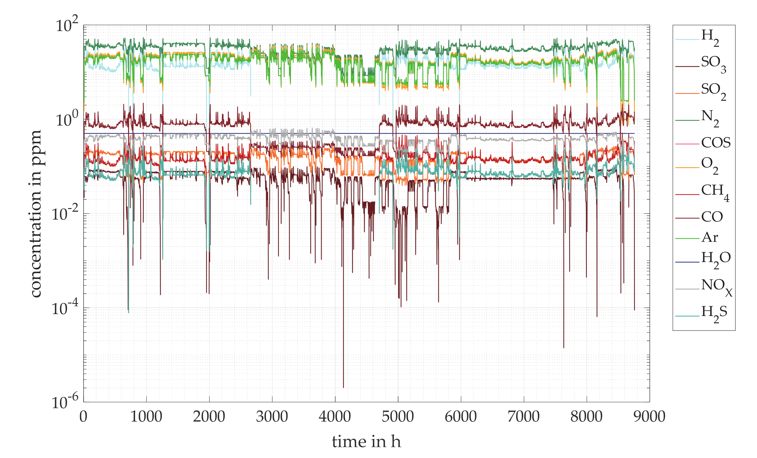
While the CO2 stream from each CO2 emitter enters the network with a constant composition, the modelled loads for the individual power plants vary substantially throughout the year (Figure 4). These load variations influence not only the overall pipeline mass flow rates in the network, but also the composition of the CO2 stream: When the individual CO2 streams are mixed, the varying pipeline mass flow rates lead to compositional variations in all pipeline sections where at least two streams are combined. As an example, the calculated variations in CO2 stream composition at the trunk line entry (pipeline segment 17 in Figure 1) are described in the following for the scenarios ”RE 27%”, “RE 45%” and “No lignite” over the course of one year (Figure 6, Figure 7 and Figure 8). Note that no chemical reactions within the CO2 stream during mixing and transport were considered.
The variations of most impurity concentrations in the baseline scenario can be described as rather moderate, with the exception of H2, CH4, H2S, COS, and CO concentrations (Figure 6). The first four impurities originate solely from the lignite-fired power plant with pre-combustion capture (Lignite PreCC) and vanish from the CO2 stream during the plant’s downtime, while CO concentrations fall to the lower level of combined CO2 streams from oxyfuel (and post-combustion capture) plants in this time period.
Modelled trunk line N2 concentrations are generally higher than O2 or Ar concentrations and predominantly follow the load and respective feed-in profile of the pre-combustion plant, as N2 is present both in CO2 streams from the oxyfuel technology and pre-combustion capture in concentrations of about 1% (Table 2). In contrast, concentrations of O2 and Ar that are absent or present only in small concentrations in streams from pre-combustion capture, respectively, are closely linked to the proportion of power generation by oxyfuel plants. Highest O2 and Ar concentrations occur when the two oxyfuel power plants are in operation. The maximum CO2 concentration is as high as 99.82%mol with a minimum concentration of 98.66%mol and a mean concentration of 99.16%mol.
As the H2O concentration in all fed-in CO2 streams was set to 50 ppmv and no chemical reactions producing or consuming H2O were considered in the calculations, the H2O concentration in the trunk line remains constant throughout the year.
Figure 7 reveals the effects of the power plants’ higher load variations on the CO2 stream composition in the scenario “RE 45%” in comparison to the base scenario: In the scenario “RE 45%”, the more continuously working power plants from the baseline scenario are substituted partly by renewable energy sources. In consequence, the power plants show more downtimes and stronger load variations compared to the baseline scenario. Overall, this results in more variable CO2 and impurity concentrations in comparison to the baseline scenario with a maximum and minimum CO2 concentration of 99.93%mol and 98.67%mol, respectively, and a mean value of 99.21%mol CO2 that is slightly higher than in the baseline scenario. Again, the downtime of the pre-combustion power plant (Lignite PreCC) can be recognised from the absence of H2, CH4, H2S, and COS in this time period. Any drop in the overall power production particularly leads to a drop in the concentrations of impurities resulting from post-combustion capture and the oxyfuel technology (such as SOx, NOx, O2, Ar) with a corresponding relative concentration increase of those impurities that originate only from pre-combustion capture (such as H2, CH4, H2S). This lignite-fired plant with pre-combustion capture runs more continuously than the other power plants in scenario “RE 45%”. In periods in which the hard coal-fired oxyfuel plant is operated flexibly (e.g., during the summer months), impurity concentration variations are more pronounced than in time periods in which predominantly the hard coal-fired plant with post-combustion capture is operated flexibly (as in mid-September to mid-November when the hard coal oxyfuel plant is switched off; Figure 4).
The variation of the impurity concentrations is noticeably smaller in the scenario “No lignite”, depicted in Figure 8, than in the other two scenarios, as the power plants—in the scenario “No lignite” only hard coal and natural gas plants—are working more continuously. Further, mainly plants with post-combustion capture are operated flexibly in this scenario. In consequence, the CO2 stream composition is “stabilised” at a certain level controlled by the lower purity of CO2 streams fed in from oxyfuel power plants. In oxyfuel plants’ shutdown periods, lower impurity concentrations occur that reflect compositions of CO2 streams from post-combustion capture. As there is no pre-combustion capture plant in this scenario, the related impurities H2, CH4, H2S, and COS are not present in the CO2 streams. CO2 concentrations fluctuate between 98.72%mol and 99.93%mol around the mean value of 99.29%mol.
3.3. Dynamics of CO2 Stream Thermophysical Properties
The considered hourly variations in CO2 stream composition introduce variations in the thermophysical properties of the CO2 stream in the different pipeline sections. The main thermophysical properties that are to be considered for pipeline design are phase behaviour (1), fluid density (2), and viscosity (3):
- (1)
- Detailed knowledge of the CO2 stream’s phase behaviour as a function of CO2 stream composition is required to calculate the minimum pressure to be maintained in order to prevent rapid phase changes or any occurrence of multiple fluid phases during normal pipeline operation.
- (2)
- The fluid density mainly determines the minimum necessary inner pipeline diameter to transport a given fluid mass per time without exceeding a maximum flow velocity of 3 m/s (cf. Section 2.2.2).
- (3)
- A higher viscosity results in a greater pressure drop along a pipe section of a given length due to an increased friction. In consequence, with higher viscosity, a higher inlet pressure and thus higher compression and pumping power are required at the capture plant outlet to transport the fluid in single phase.
As a direct result of the varying CO2 stream composition, density and viscosity values also vary, reflecting the mixing of different impure CO2 streams in the collection network. Modelled maximum viscosity values are very similar for all three scenarios as exemplarily shown for the trunk line entry in Figure 9, even though the viscosities in each scenario show very distinct time courses as well as specific average and minimum values. Modelled density variations (data not shown) exhibit a close similarity to the viscosity variations.
A higher feed-in from oxyfuel and pre-combustion plants leads to a temporal occurrence of CO2 streams with higher impurity concentrations, resulting in streams with lower densities and viscosities. In the contrary, in the summer period, in particular in the scenario “No lignite”, when only power plants equipped with post-combustion capture feed in CO2 streams, trunk line CO2 streams are of higher purity and, hence, also of higher density and viscosity than in the other time periods. Density and viscosity values depend mainly on the total CO2 purity, i.e., on the CO2 concentration, rather than on the specific CO2 stream composition. Overall, the modelled effect of CO2 purity variations on viscosities and densities is small.
4. Discussion
4.1. CO2 Stream Composition
4.1.1. CO2 Emitters and Capture Processes
The impurities under consideration in this study were selected according to each impurity’s abundance in the CO2 streams, its reactivity, and its impact on the thermodynamic and transport properties of the CO2 stream. Other impurities that may be of toxicological concern, such as trace metals, or may lead to specific technical challenges, such as particulates (e.g., [40]), were not considered in this study. For each emitter, the CO2 stream composition was assumed to be constant over time in order to focus this study on the effects of CO2 stream mixing. For the same reason, only one exemplary state-of-the-art process configuration for each capture technology was selected in the modelling of the CO2 emitters, i.e., flue gas scrubbing with monoethanolamine (MEA) in case of post-combustion capture, as the focus of this study was not on capture technologies. Rather CO2 emitters and their “output” CO2 stream compositions were used to investigate impacts of the CO2 emitters’ dynamic operational behaviour on CO2 stream composition and mass flow rates in a pipeline network. Numerous capture processes and their optimizations are described in the literature (e.g., [41,42,43]). The selected CO2 stream compositions (Table 2 in Section 2.1.2) can be regarded as representative for each considered capture technology. However, strictly speaking, they are only examples out of many possible compositions. With a positive or negative impact on plant complexity and economic efforts, higher or lower concentrations of impurities can be realised. A need for higher or lower impurity concentrations may result from specific requirements during CO2 transport, injection, and/or storage. An overall optimisation of the CO2 stream composition for a specific CCS chain or network must ensure a safe CCS operation, while avoiding unnecessary purification steps (from an energetic, economic, and technological point of view). Such an optimisation has to be based on a comprehensive consideration of potential impacts of impurities along a whole CCS chain (e.g., [24,39,44]).
In all energy mix scenarios, H2O concentration was limited to 50 ppmv for all fed-in CO2 streams (i) to avoid the formation and condensation of an aqueous phase within the CO2 transport system and (ii) to reduce the formation and condensation of nitric and sulfuric acid for limiting and controlling pipe corrosion (e.g., [24]). For real (i.e., non-generic) CCS projects, a potential hydrate formation (in case of rapid cooling during depressurization) must also be considered to specify the H2O concentration. The ISO standard “Carbon dioxide capture, transportation and geological storage—Pipeline transportation systems (ISO 27913:2016(E))” [45] gives indicative H2O levels in CO2 streams of 20 to 630 ppmv (for corrosion control) and of < 200 ppmv (to prevent hydrate formation). The acceptable H2O concentration for corrosion control strongly depends on the reactivity and concentrations of all impurities in the CO2 stream. Relatively high H2O concentrations may be acceptable in very pure CO2 streams or in streams containing impurities with reducing properties (e.g., from pre-combustion capture or H2 production, cf. [46]). In contrast, low H2O concentrations may be required for corrosion control in CO2 streams containing oxidizing and/or acid-forming impurities such as O2, SOx, NOx (e.g., [12,45]).
The CO2 stream compositions of the different plants and capture facilities listed in Table 2 were used irrespective of the plants’ operational mode, i.e., same compositions were assumed for full and part load operation. Some approaches have been reported in the literature to exactly model the fate of different impurities during selected capture processes and compression (e.g., [47]). Modelling these chemical multi-component systems with a CO2 phase and an aqueous phase at different pressure and temperature levels is not trivial, as for example, the interaction between NOx and SO2 during capture and compression is not yet fully understood and experimental kinetic data are missing for some potential reaction pathways (e.g., [47]). For this study, SO2: SO3 ratios of 2.5 and 1:1 were used for CO2 streams containing SOx from oxyfuel plants and PCC plants, respectively (Table 2). Knowing the exact SO3 concentration would be beneficial as SO3 directly reacts with H2O in the CO2 stream or dissolves in an aqueous phase to produce sulfuric acid (H2SO4), a highly corrosive acid. In contrast, SO2 oxidation in the CO2 stream by O2 is slow, potentially leading to only a moderate SO3 production from SO2 during pipeline transport (e.g., [48]).
4.1.2. Variability of CO2 Stream Composition and its Implication for Transport, Injection, and Storage
To assess potential impacts of variations in impurity concentrations, the variation frequency and amplitude as well as the occurrence of specific impurity levels throughout the year have to be considered. These parameters differ in the energy mix scenarios considered (Figure 10) with implications for CO2 stream reactivity and thermophysical properties. From Figure 10, it can be seen that the maximum (and minimum) concentrations occur at a few hours per year only (except when impurities are temporarily absent from the CO2 stream). In comparison to the base scenario “RE 27%”, relative concentrations of impurities with reducing properties (e.g., H2, CO) are generally higher in scenario “RE 45%” as the lignite-fired power plants (including the one equipped with pre-combustion capture) are the last to be shut down when the electricity demand can be met to a large part from renewable energy sources.
On the contrary, e.g., SO3 concentrations temporarily drop to zero when all power plants with post-combustion capture or the oxyfuel technology are offline. In the scenario “No lignite”, no plant with pre-combustion capture is operating so that, e.g., no H2 is present in the CO2 streams of this scenario. Furthermore, changes in CO2 stream composition are more moderate in the scenario “No lignite”, always containing a similar set of impurities but with varying concentrations.
The calculated variations in CO2 stream compositions lead to small changes in CO2 stream viscosity and density at the considered transport temperature of 288 K and the calculated pipeline pressures between about 5.5 and 12.5 MPa, i.e., the CO2 stream is present as a dense-phase (liquid) fluid in all considered scenarios. At transport temperatures closer to the critical temperature, changes in CO2 stream composition would result in more pronounced changes in viscosity and density (cf. [49,50]). In addition, higher impurity concentrations and related larger variations in CO2 stream composition will cause larger viscosity variations than those modelled in this study.
Whereas for most impurities, the CO2 stream’s thermophysical properties are predominantly a function of the overall CO2 purity, i.e., the CO2 concentration (e.g., [50]), the chemical reactivity of all individual impurities present in the CO2 stream controls potential chemical impacts along the whole CCS chain. For example, as there is no plant with pre-combustion capture in the scenario “No lignite”, e.g., no H2 is present in the CO2 streams of this scenario. In consequence, redox properties of CO2 streams in this scenario are very different, i.e., streams are more oxidizing here than in the other two scenarios. For example in steel corrosion studies, impurities with reducing properties led to other corrosion products and a lower corrosion rate than impurities with oxidising and/or acid-forming properties (e.g., [51]). Mixing CO2 streams with reducing and oxidizing properties further increased steel corrosion [51]. This may be related to cross-chemical reactions between the different impurities in a CO2 stream, leading to a formation of strong acids (cf. [52]). In contrast, corrosion experiments with an alternation of CO2 streams containing reducing or oxidizing impurities gave corrosion effects similar to those observed in experiments with oxidizing impurities in the CO2 stream only [51].
4.2. Mass Flow Rates and Pipeline Capacity Utilisation
In this study, the main purpose for setting-up energy mix scenarios was to analyse the sensitivity of CO2 stream compositions and mass flow rates towards changes of the feed CO2 streams’ properties as pointed out above. In consequence, for example, the unrealistic deployment of the natural gas fired plants with post-combustion capture (NGCC-PCC2, resp. -PCC3) with extremely few full load hours in the energy mix scenarios was deliberately accepted to generate extreme values of mass flow rate and composition variation. The scenarios “RE 45%” and “No lignite” represent only two of many possibilities of future developments in Germany’s energy mix. Phasing out power generation from lignite and increasing the share of renewable power production are two measures included in the Government’s Climate Action Programme 2050 [34]. Due to various influencing factors for the development of the future national energy mix, an assessment of how realistic these scenarios are cannot be made. In 2018, power production from renewable energy sources accounted for approx. 37.8% of Germany’s power production, increasing to 42.1% in 2019 [53]. The overall methodology can be adopted to other countries when respective data on power production and industrial plant characteristics are available.
The high dynamics in the share of energy production from renewable energy sources raises the issue of how to define the pipeline design capacity, in particular the trunk line design capacity. Comparing the annual duration curves in the energy mix scenarios (Figure 11), it is striking that maximum as well as minimum pipeline mass flow rates occur only for a few hundred hours per year. Maximum pipeline mass flow rates represent time periods with a low renewable power production and a high power production from conventional fossil-fired power plants to meet the demand, whereas minimum pipeline mass flow rates represent times of high renewable energy production. Thus, if the pipeline (in particular the trunk line) is designed for transporting the entire amount of CO2 captured, its capacity will only partially be used during most of the year, thereby decreasing transport efficiency both economically and energetically. This effect is most pronounced in scenario “RE 45%” (Figure 11) in which the variations (amplitudes) of pipeline mass flow rates are significantly larger than in the other two energy mix scenarios.
Options for increasing the pipeline capacity utilisation and thus the overall transport efficiency may include reducing the pipeline design capacity and considering only partial transport (and consequently also partial capture) during peak load periods. If captured, peak load streams may be stored temporarily until they can be fed into the transport network (e.g., during minimum load periods). For temporary storage, considered options may include short-term storage in CO2 absorbents or by line packing (e.g., [19]) or storage in a buffer store (tank or rock formation, e.g., [16]). Furthermore, in CCS networks like the ones considered in this study, source and network management may provide alternative means to reduce the variability in mass flow rates (e.g., [16]).
5. Conclusions
The simulations of mass flow rates and CO2 stream compositions in several energy mix scenarios reflecting possible future changes in Germany’s energy mix show that there can be substantial variations in those parameters with potential implications for pipeline and storage design and operation. Over a CCS project’s assumed lifetime of about 30 years, CO2 sources and/or their operational patterns as well as capture technologies may evolve and thus CO2 stream composition and fed-in mass flow rates and the variations thereof will equally do. Thus, for example, future developments in CO2 supply should be accounted for in order to optimise pipeline network design and ensure a sustained cost-efficient pipeline utilisation over the entire pipeline lifetime. With respect to variations in the CO2 stream composition, each pipeline segment has to be carefully designed and monitored during operation to avoid leaving its safe operation window. Overall, future developments of CO2 stream composition and mass flow rate variability and their impacts on all parts of the CCS network should be carefully considered in CCS project planning. Similar considerations apply to CO2 transport networks that are part of CO2 capture and utilisation systems.
Author Contributions
Study conceptualization, H.R., S.-L.K., and M.P.; methodology, S.-L.K., M.P., and S.S.; software, M.P.; investigation, M.P. and S.-L.K.; writing—original draft preparation, M.P., S.-L.K., and H.R.; writing—review and editing, M.P., S.-L.K., H.R., and A.K.; visualization, S.-L.K. and M.P.; supervision, A.K., S.S., and H.R.; funding acquisition, A.K., S.S., and H.R. All authors have read and agreed to the published version of the manuscript.
Funding
This work was done as part of the project CLUSTER funded by the Federal Ministry for Economic Affairs and Energy on the basis of a decision by the German Bundestag (Grant Numbers 03ET7031A to C).
Acknowledgments
The authors acknowledge the fruitful collaboration and stimulating discussions with the entire team of the CLUSTER project. We also would like to thank the three anonymous reviewers for their constructive comments that helped to improve the manuscript. In addition, the authors gratefully acknowledge the proofreading by S. Stadler (BGR).
Conflicts of Interest
The authors declare no conflict of interest. The funders had no role in the design of the study, in the collection, analyses, or interpretation of data, in the writing of the manuscript, or in the decision to publish the results.
References
- Chandel, M.; Pratson, L.; Williams, E. Potential economies of scale in CO2 transport through use of a trunk pipeline. Energy Convers. Manag. 2010, 51, 2825–2834. [Google Scholar] [CrossRef]
- Zero Emission Platform—ZEP. The Costs of CO2 Capture, Transport and Storage; Report; Zero Emission Platform: Brussels, Belgium, 2011. [Google Scholar]
- IEAGHG. Carbon Capture and Storage Cluster Projects: Review and Future Opportunities; Technical Report 2015/03; IEA Environmental Projects: Cheltenham, UK, 2015. [Google Scholar]
- Gomes, J.F.P. Carbon Dioxide Capture and Sequestration; Nova Publishers Inc.: New York, NY, USA, 2013. [Google Scholar]
- Bazzanella, A.; Krämer, D. Technologien für Nachhaltigkeit und Klimaschutz—Chemische Prozesse und stoffliche Nutzung von CO2; Report; DECHEMA Gesellschaft für Chemische Technik und Biotechnologie e.V.: Frankfurt am Main, Germany, 2017. [Google Scholar]
- Directive 2009/31/EC of the European Parliament and the Council of 23 April 2009 on the Geological Storage of Carbon Dioxide and Amending Council Directive 85/337/EEC, European Parliament and Council Directives 2000/60/EC, 2001/80/EC, 2004/35/EC, 2006/12/EC und 2008/1/EC and Regulation (EC) No. 1013/2006. Available online: eur-lex.europa.eu/legal-content/EN/TXT/?uri=CELEX%3A32009L0031 (accessed on 8 April 2019).
- ISO 27917:2017. Carbon Dioxide Capture, Transportation and Geological Storage—Vocabulary—Cross Cutting Terms. Available online: www.iso.org/obp/ui/#iso:std:iso:27917:ed-1:v1:en (accessed on 5 February 2020).
- Peletiri, S.P.; Rahmanian, N.; Mujtaba, I.M. CO2 Pipeline Design: A Review. Energies 2018, 11, 2184–2208. [Google Scholar] [CrossRef] [Green Version]
- Martynov, S.B.; Daud, N.K.; Mahgerefteh, H.; Brown, S.; Porter, R.T.J. Impact of stream impurities on compressor power requirements for CO2 pipeline transportation. Int. J. Greenh. Gas Control 2016, 54, 652–661. [Google Scholar] [CrossRef]
- Munkjord, S.T.; Hammer, M.; Lovseth, S.W. CO2 transport: Data and models—A review. Appl. Energy 2016, 169, 499–523. [Google Scholar] [CrossRef]
- IEAGHG. Effects of Impurities on Geological Storage of CO2; Technical Report 2011/4; IEA Environmental Projects: Cheltenham, UK, 2011. [Google Scholar]
- Halseid, M.; Dugstad, A.; Morland, B. Corrosion and bulk phase reactions in CO2 transport pipelines with impurities: Review of recent published studies. Energy Proc. 2014, 63, 2557–2569. [Google Scholar] [CrossRef] [Green Version]
- Talman, S. Subsurface geochemical fate and effects of impurities contained in a CO2 stream injected into a deep saline aquifer: What is known. Int. J. Greenh. Gas Control 2015, 40, 267–291. [Google Scholar] [CrossRef]
- Brouwer, A.S.; van den Broek, M.; Seebregts, A.; Faaij, A. Operational flexibility and economics of power plants in future low-carbon power systems. Appl. Energy 2015, 156, 107–128. [Google Scholar] [CrossRef] [Green Version]
- Mechleri, E.; Fennell, P.S.; Mac Dowell, N. Optimisation and evaluation of flexible operation strategies for coal- and gas-CCS power stations with a multi-period design approach. Int. J. Greenh. Gas Control 2017, 59, 24–39. [Google Scholar] [CrossRef] [Green Version]
- IEAGHG. Operational Flexibility of CO2 Transport and Storage; Technical Report 2016/4; IEA Environmental Projects: Cheltenham, UK, 2016. [Google Scholar]
- Spitz, T.; Chalmers, H.; Ascui, F.; Lucquiaud, L. Operating flexibility of CO2 injection wells in future low carbon energy system. Energy Proc. 2017, 114, 4797–4810. [Google Scholar] [CrossRef]
- Spitz, T.; Avagyan, V.; Ascui, F.; Bruce, A.R.W.; Chalmers, H.; Lucquiaud, M. On the variability of CO2 feed flows into CCS transportation and storage. Int. J. Greenh. Gas Control 2018, 74, 296–311. [Google Scholar] [CrossRef]
- Wetenhall, B.; Race, J.; Aghajani, H.; Sanchez Fernandez, E.; Naylor, M.; Lucquiaud, M. Considerations in the development of flexible CCS networks. Energy Proc. 2017, 114, 6800–6812. [Google Scholar] [CrossRef] [Green Version]
- Lubenau, U.; Pumpa, M.; Schütz, S.; Barsch, M. CLUSTER—Einfluss von CO2-Begleitkomponenten auf die Auslegung und Gestaltung des Transportnetzes und der Obertageanlage; Final Report; DBI Gas- und Umwelttechnik GmbH: Leipzig, Germany, 2019; Available online: www.bgr.bund.de/CLUSTER-EN (accessed on 21 October 2019).
- CLUSTER—Impacts of Impurities in CO2 Streams Captured from Different Emitters in a Regional Cluster on Transport, Injection and Storage–Project Website. Available online: www.bgr.bund.de/CLUSTER-EN (accessed on 12 December 2019).
- Umweltbundesamt–UBA. Kohlendioxidemissionen. Available online: www.umweltbundesamt.de/daten/klima/treibhausgas-emissionen-in-deutschland/kohlendioxid-emissionen#kohlendioxid-emissionen-im-vergleich-zu-anderen-treibhausgasen (accessed on 1 September 2020).
- Kather, A.; Paschke, B.; Kownatzki, S. COORAL—Prozessgasdefinition, Transportnetz und Korrosion; Final Report; Hamburg Technical University: Hamburg, Germany, 2013; Available online: www.bgr.bund.de/COORAL (accessed on 23 March 2016).
- Rütters, H.; Stadler, S.; Bäßler, R.; Bettge, D.; Jeschke, S.; Kather, A.; Lempp, C.; Lubenau, U.; Ostertag-Henning, C.; Schmitz, S. Towards an optimization of the CO2 stream composition—A whole chain approach. Intern. J. Greenh. Gas Control 2016, 54, 682–701. [Google Scholar] [CrossRef]
- ENTSOE-E. European Network of Transmission System Operators for Electricity. Actual Generation per Production Type. Available online: www.entsoe.eu (accessed on 3 May 2016).
- European Energy Exchanges AG. EEX Transparency Platform. Available online: www.eex-transparency.com (accessed on 18 January 2016).
- Pyc, I. VDE-Studie: Erneuerbare Energie braucht flexible Kraftwerke—Szenarien bis 2020; Presentation of 21 November 2013. Available online: www.vde.com/de/etg/publikationen/studien/studie-flex (accessed on 26 June 2015).
- Steck, M.; Mauch, W. Technische Anforderungen an neue Kraftwerke im Umfeld dezentraler Stromerzeugung. In Paper zum 10. Symposium Energieinnovation; Forschungsstelle für Energiewirtschaft e.V.: Graz, Austria, 2008. [Google Scholar]
- Weber, C. Management der Stromerzeugung; Lecture slides; Universität Duisburg Essen: Duisburg, Germany, 2014. [Google Scholar]
- Bauersfeld, S. Dynamische Modellierung des Gaspfades eines Gesamt-IGCC-Kraftwerkes auf Basis des SFG-Verfahrens. Ph.D. Thesis, Technische Universität Bergakademie Freiberg, Freiberg, Germany, 2014. [Google Scholar]
- Umweltbundesamt—UBA. Merkblatt über die besten verfügbaren Techniken in der Zement-, Kalk- und Magnesiumoxidindustrie. Dessau, 2010. Available online: www.bvt.umweltbundesamt.de (accessed on 10 March 2016).
- Umweltbundesamt—UBA. Merkblatt über die Besten Verfügbaren Techniken für Mineralöl- und Gasraffinerien. Dessau, 2003. Available online: www.bvt.umweltbundesamt.de (accessed on 2 December 2016).
- Umweltbundesamt—UBA. Merkblatt über die Besten Verfügbaren Techniken in der Eisen- und Stahlerzeugung. Dessau, 2012. Available online: www.bvt.umweltbundesamt.de (accessed on 11 February 2015).
- Bundesregierung. Climate Action Plan 2050; Federal Ministry for the Environment, Nature Conservation, Building and Nuclear Safety (BMUB), 2016. Available online: www.bmu.de/publikation/climate-action-plan-2050 (accessed on 1 September 2020).
- Bundesministerium für Wirtschaft und Energie—BMWi. Erneuerbare Energien in Zahlen 2017. Available online: www.bmwi.de/Redaktion/DE/Publikationen/Energie/erneuerbare-energien-in-zahlen-2017.pdf (accessed on 17 September 2020).
- Lubenau, U.; Schmitz, S.; Rockmann, R.; Schütz, S.; Käthner, R. CO2-Reinheit für die Abscheidung und Lagerung (COORAL); Final Report; DBI Gas- und Umwelttechnik GmbH: Leipzig, Germany, 2013; Available online: www.bgr.bund.de/COORAL (accessed on 1 August 2015).
- Lemmon, E.; Huber, M.; McLinden, M. NIST Standard Reference Database 23: Reference Fluid Thermodynamic and Transport Properties—REFPROP, Version 9.1; National Institute of Standards and Technology: Gaithersburg, MD, USA, 2013. [Google Scholar]
- American Petroleum Institute—API. Recommended Practice for Design and Installation of Offshore Production Platform Piping Systems (API RP 14E); American Petroleum Institute: Washington, DC, USA, 1991. [Google Scholar]
- Brunsvold, A.; Jakobsen, J.P.; Mazzetti, M.J.; Skaugen, G.; Hammer, M.; Eickhoff, C.; Neele, F. Key findings and recommendations from the IMPACTS project. Int. J. Greenh. Gas Control 2016, 54, 588–598. [Google Scholar] [CrossRef]
- Thitakamol, B.; Veawab, A.; Aroonwilas, A. Environmental impacts of absorption-based CO2 capture unit for post-combustion treatment of flue gas from coal-fired power plant. Int. J. Greenh. Gas Control 2007, 1, 318–342. [Google Scholar] [CrossRef]
- Kather, A.; Syrigos, S.; Dickmeis, J. ADECOS-Komponenten: Oxyfuel-Komponentenentwicklung und -Prozessoptimierung. Projektbereich 2: Gasbehandlung; Final Report; Hamburg Technical University: Hamburg, Germany, 2015. [Google Scholar]
- IEAGHG. Improvement in Power Generation with Post-Combustion Capture of CO2; Technical Report PH4/33; IEA Environmental Projects: Cheltenham, UK, 2004. [Google Scholar]
- Keller, D.; Scholz, M.H. Development perspectives of lignite based IGCC plants with CCS. VGB PowerTech 2010, 90, 30–34. [Google Scholar]
- Porter, R.T.J.; Mahgerefteh, H.; Brown, S.; Martynov, S.; Collard, A.; Woolley, R.B.; Fairweather, M.; Falle, S.A.E.G.; Wareing, C.J.; Nikolaidis, I.K.; et al. Techno-economic assessment of CO2 quality effect on its storage and transport: CO2QUEST: An overview of aims, objectives and main findings. Int. J. Greenh. Gas Control 2016, 54, 662–681. [Google Scholar] [CrossRef] [Green Version]
- ISO 27913:2016 Carbon dioxide capture, transportation and geological storage—Pipeline transportation systems. Available online: https//www.iso.org/obp/ui/#iso:std:iso:27913:ed-1:v1:en (accessed on 5 February 2020).
- De Visser, E.; Hendriks, C.; Barrio, M.; Mølnvik, M.J.; de Koeijer, G.; Liljemark, S.; LeGallo, Y. Dynamis CO2 quality recommendations. Int. J. Greenh. Gas Control 2008, 2, 478–484. [Google Scholar] [CrossRef]
- Ajdari, S.; Normann, F.; Andersson, K.; Johnsson, F. Modeling the nitrogen and sulfur chemistry in pressurized flue gas systems. Ind. Eng. Chem. Res. 2015, 54, 1216–1227. [Google Scholar] [CrossRef]
- Rütters, H.; Abbasi, N.; Amshoff, P.; Barsch, M.; Bäßler, R.; Bettge, D.; Engel, F.; Fischer, S.; Fuhrmann, L.; Grunwald, N.; et al. Auswirkungen der Begleitstoffe in den abgeschiedenen CO2-Strömen unterschiedlicher Emittenten eines regionalen Clusters auf Transport, Injektion und Speicherung (CLUSTER)—Abschlusssynthese; Synthesis Report; Bundesanstalt für Geowissenschaften und Rohstoffe: Hannover, Germany, 2019; Available online: www.bgr.bund.de/CLUSTER-EN (accessed on 12 December 2019).
- Nazeri, M.; Chapoy, A.; Burgass, R.; Tohidi, B. Viscosity of CO2-rich mixtures from 243 K to 423 K at pressures up to 155 MPa: New experimental viscosity data and modelling. J. Chem. Thermodyn. 2018, 118, 100–114. [Google Scholar] [CrossRef]
- Wetenhall, B.; Aghajani, H.; Chalmers, H.; Benson, S.D.; Ferrari, M.-C.; Li, J.; Race, J.M.; Singh, P.; Davison, J. Impact of CO2 impurity on CO2 compression, liquefaction and transportation. Energy Proc. 2014, 63, 2764–2778. [Google Scholar] [CrossRef] [Green Version]
- Bettge, D.; Bäßler, R.; Le, Q.-H.; Kranzmann, A. CLUSTER—Werkstoffauswahl und Festlegung von Obergrenzen für Verunreinigungen in variierenden CO2-Strömen auf Grund von realitätsnahen Korrosionsexperimenten; Final Report; Bundesanstalt für Materialforschung und -prüfung: Berlin, Germany, 2019; Available online: www.bgr.bund.de/CLUSTER-EN (accessed on 12 December 2019).
- Morland, B.H.; Dugstad, A.; Tjelta, M.; Svennigsen, G. Formation of strong acids in dense phase CO2. In Proceedings of the Corrosion 2018, Phoenix, AZ, USA, 15–19 April 2018; NACE International: Houston, TX, USA, 2018. NACE 2018–11429. [Google Scholar]
- Umweltbundesamt—UBA: Erneuerbare Energien in Zahlen 2019. Available online: www.umweltbundesamt.de/themen/klima-energie/erneuerbare-energien/erneuerbare-energien-in-zahlen (accessed on 5 February 2020).
Figure 1.
Schematic representation of the transport network (dimensions not to scale). The regional cluster of the 11 CO2 emitters is 75 km in diameter, while the trunk pipeline has a length of 300 km in its onshore part. Numbers on the pipeline segments are identifiers for further considerations.
Figure 1.
Schematic representation of the transport network (dimensions not to scale). The regional cluster of the 11 CO2 emitters is 75 km in diameter, while the trunk pipeline has a length of 300 km in its onshore part. Numbers on the pipeline segments are identifiers for further considerations.

Figure 2.
Net efficiency over the rated thermal input of the considered power plants equipped with CO2 capture.
Figure 2.
Net efficiency over the rated thermal input of the considered power plants equipped with CO2 capture.

Figure 3.
CO2 emissions and resulting pipeline mass flow rates of industrial plants with additional CO2 emissions due to CO2 capture.
Figure 3.
CO2 emissions and resulting pipeline mass flow rates of industrial plants with additional CO2 emissions due to CO2 capture.

Figure 4.
Stacked pipeline mass flow rates in the three examined energy mix scenarios during one year: (A) “RE 27%”, (B) “RE 45%” and (C) “No lignite”. (Note that the plants NGCC PCC3, Hard Coal PCC2, and Hard Coal Oxy2 occur only in scenario “No lignite”).
Figure 4.
Stacked pipeline mass flow rates in the three examined energy mix scenarios during one year: (A) “RE 27%”, (B) “RE 45%” and (C) “No lignite”. (Note that the plants NGCC PCC3, Hard Coal PCC2, and Hard Coal Oxy2 occur only in scenario “No lignite”).

Figure 5.
Relative full load hours (A) and pipeline mass flow rates (B) in the energy mix scenarios (the baseline scenario is scenario “RE 27%”).
Figure 5.
Relative full load hours (A) and pipeline mass flow rates (B) in the energy mix scenarios (the baseline scenario is scenario “RE 27%”).

Figure 6.
Simulated variation (hourly averages) of individual impurity concentrations within the CO2 stream at the entry of the trunk pipeline throughout one year (= 8760 h) for the baseline scenario “RE 27%” (T = 288 K, pinlet ≤ 12.33 MPa; note that COS concentration data are hidden behind the H2S data as its concentration values are identical to those of H2S throughout the year).

Figure 7.
Simulated variation (hourly averages) of individual impurity concentrations within the CO2 stream at the entry of the trunk pipeline throughout one year (= 8760 h) for the scenario “RE 45%” (T = 288 K, pinlet ≤ 12.41 MPa; note that COS concentration data are hidden behind the H2S data as its concentration values are identical to those of H2S throughout the year).

Figure 8.
Simulated variation (hourly averages) of individual impurity concentrations at the entry of the trunk pipeline throughout one year (= 8760 h) for the scenario “No lignite” (T = 288 K, pinlet ≤ 12.62 MPa; note that COS concentration data are hidden behind the H2S data as its concentration values are identical to those of H2S throughout the year).

Figure 9.
Viscosity variations at the trunk line entry calculated from the fed-in variable pipeline mass flow rates and CO2 stream compositions (hourly averages) throughout one year (= 8760 h) for the scenarios “RE 27%”, “RE 45%”, and “No lignite” (note that the figure is zoomed in on the y-axis).
Figure 9.
Viscosity variations at the trunk line entry calculated from the fed-in variable pipeline mass flow rates and CO2 stream compositions (hourly averages) throughout one year (= 8760 h) for the scenarios “RE 27%”, “RE 45%”, and “No lignite” (note that the figure is zoomed in on the y-axis).

Figure 10.
Modelled occurrence of different impurity concentrations at the trunk line entry per year—a comparison between the energy mix scenarios. (Occurrences of H2, CO, O2, SO2, and SO3 concentrations are given in (A–E), respectively.)
Figure 10.
Modelled occurrence of different impurity concentrations at the trunk line entry per year—a comparison between the energy mix scenarios. (Occurrences of H2, CO, O2, SO2, and SO3 concentrations are given in (A–E), respectively.)

Figure 11.
Modelled occurrence of different pipeline mass flow rates at the trunk line entry per year—a comparison between the energy mix scenarios.
Figure 11.
Modelled occurrence of different pipeline mass flow rates at the trunk line entry per year—a comparison between the energy mix scenarios.


Table 1.
Considered power plants and industrial plants with respective CO2 capture technologies.
| Plant | Capture Technologies | Plant Size | Abbreviation |
|---|---|---|---|
| Hard coal fired power plants | Post Combustion | 431.9 MW | Hard Coal PCC |
| Oxyfuel | 431.9 MW | Hard Coal Oxy | |
| Lignite fired power plants | Post Combustion | 410.3 MW | Lignite PCC |
| Oxyfuel | 466.6 MW | Lignite Oxy | |
| Pre Combustion | 360 MW | Lignite PreCC | |
| Natural gas combined cycle plants | Post Combustion | 633.5 MW | NGCC PCC1 |
| Post Combustion | 633.5 MW | NGCC PCC2 | |
| Iron and steel mill | Post Combustion | 2.5 Mt steel/year | Steel PCC |
| Cement plants | Post Combustion | 3000 t clinker/day | Cem. PCC |
| Oxyfuel | 3000 t clinker/day | Cem. Oxy | |
| Refinery | Post Combustion | 30000 t crude oil/day | Ref. PCC |
Table 2.
Considered CO2 stream composition of each CO2 emitter and CO2 capture technology after compression (p = 11 MPa, T = 313 K) (PCC: post-combustion capture, PreCC: pre-combustion capture).
Table 2.
Considered CO2 stream composition of each CO2 emitter and CO2 capture technology after compression (p = 11 MPa, T = 313 K) (PCC: post-combustion capture, PreCC: pre-combustion capture).
| Component | PCC Plants in vol% | Oxyfuel Power Plantsin vol% | Oxyfuel Cement Plant in vol% | PreCC Power Plant in vol% |
|---|---|---|---|---|
| CO2 | 99.931 | 98.0029 | 98.0049 | 98.0039 |
| O2 | 0.015 | 0.67 | 0.59 | |
| N2 | 0.0225 | 0.71 | 0.84 | 0.9005 |
| Ar | 0.0225 | 0.59 | 0.54 | 0.03 |
| H2O | 0.005 | 0.005 | 0.005 | 0.005 |
| SO2 | (0.0005) * | 0.005 | ||
| SO3 | (0.0005) * | 0.002 | ||
| NOx | 0.002 | 0.01 | 0.01 | |
| CO | 0.001 | 0.005 | 0.01 | 0.04 |
| H2 | 1.0006 | |||
| CH4 | 0.01 | |||
| H2S | 0.005 | |||
| COS | 0.005 |
*: No SOx in CO2 streams captured on cement plants with PCC (see text for explanation).
Table 3.
Pipeline mass flow rates (total, minimum, maximum, average) in the scenarios “RE 27%” (baseline), “RE 45%” and “No lignite”.
Table 3.
Pipeline mass flow rates (total, minimum, maximum, average) in the scenarios “RE 27%” (baseline), “RE 45%” and “No lignite”.
| Scenario | “RE 27%” | “RE 45%” | “No Lignite” |
|---|---|---|---|
| Total pipeline mass flow rate [Mt/a] | 19.69 | 16.32 | 17.91 |
| Max. pipeline mass flow rate [t/h] | 3155.4 | 3101.5 | 2921.8 |
| Min. pipeline mass flow rate [t/h] | 1032.5 | 604.1 | 997.4 |
| Average pipeline mass flow rate [t/h] | 2247.4 | 1863.2 | 2044.1 |
© 2020 by the authors. Licensee MDPI, Basel, Switzerland. This article is an open access article distributed under the terms and conditions of the Creative Commons Attribution (CC BY) license (http://creativecommons.org/licenses/by/4.0/).
Share and Cite
MDPI and ACS Style
Kahlke, S.-L.; Pumpa, M.; Schütz, S.; Kather, A.; Rütters, H. Potential Dynamics of CO2 Stream Composition and Mass Flow Rates in CCS Clusters. Processes 2020, 8, 1188. https://0-doi-org.brum.beds.ac.uk/10.3390/pr8091188
AMA Style
Kahlke S-L, Pumpa M, Schütz S, Kather A, Rütters H. Potential Dynamics of CO2 Stream Composition and Mass Flow Rates in CCS Clusters. Processes. 2020; 8(9):1188. https://0-doi-org.brum.beds.ac.uk/10.3390/pr8091188
Chicago/Turabian StyleKahlke, Sven-Lasse, Martin Pumpa, Stefan Schütz, Alfons Kather, and Heike Rütters. 2020. "Potential Dynamics of CO2 Stream Composition and Mass Flow Rates in CCS Clusters" Processes 8, no. 9: 1188. https://0-doi-org.brum.beds.ac.uk/10.3390/pr8091188
Note that from the first issue of 2016, this journal uses article numbers instead of page numbers. See further details here.