Adaptive Monitoring of Biotechnological Processes Kinetics

Abstract

In this paper, an approach for the monitoring of biotechnological process kinetics is proposed. The kinetics of each process state variable is presented as a function of two time-varying unknown parameters. For their estimation, a general software sensor is derived with on-line measurements as inputs that are accessible in practice. The stability analysis with a different number of inputs shows that stability can be guaranteed for fourth- and fifth-order software sensors only. As a case study, the monitoring of the kinetics of processes carried out in stirred tank reactors is investigated. A new tuning procedure is derived that results in a choice of only one design parameter. The effectiveness of the proposed procedure is demonstrated with experimental data from Bacillus subtilis fed-batch cultivations.

1. Introduction

Monitoring of the main variables and parameters of biotechnological processes is of key importance for processes investigations and control, especially in industrial installations, where a limited number of measurements is available [1,2].

A widely used approach for process monitoring is model-based software sensor (SS) design [3,4]. The operational model has to be (i) as accurate as possible to mimic the main characteristics and dynamics of the process, and (ii) simple enough for a monitoring and control design. Such an operational model was proposed by Bastin and Dochain [4] as the general dynamical model (GDM) of bioprocesses in stirred tank reactors (STR). Approaches based on GDM software sensors are widely applied simultaneously with other approaches for nonlinear systems, such as extended Kalman and Luenberger filters [5,6,7,8], moving horizon [9,10] neural-network based observers [11], high-gain approach [12], multirate observers [13], sliding mode-observers [14,15], interval SS [16], cascade SS [17,18,19], and joint estimation of state variables and parameters [1,20,21], among others.

Usually, the software sensors are designed using operational models with constant yield coefficients [4,12,15,20,21]. For many industrial biotechnological processes, like wastewater treatment and processes in inhomogeneous mediums, the reproducibility is poor [18,22]. Hence, the assumption of a constant yield coefficient leads to inexact results because of considerable changes of these parameters during a process or within different production batches. This change is due to adaptations of metabolic pathways, protein expression pattern, and random mutations of organisms, as well as the occurrence and dynamics of population heterogeneities in single species, especially in multispecies bioprocesses [23,24].

Although it is biologically self-evident that such coefficients are not constant, there are only a few examples of yield coefficients or maximum uptake rates that have been considered as dynamic parameters in the literature. As an example, for Escherichia coli fed-batch processes, the dynamic decrease of the maximum uptake rates for the substrate (glucose) and oxygen was modelled kinetically based on experimental observations [25,26], although, in this case, new parameters were added to the complex model, which decreased the identifiability of the parameters. Also, in our previous studies [18,22,23], the functional relations between the estimated and measured variables and parameters were determined for each concrete case.

The authors of [27] considered a class of aerobic processes for which on-line measurements of the oxygen consumption rate were available. A linear structure of a software sensor was derived from these data. Estimates of biomass concentration and two kinetic parameters (biomass growth rate and yield coefficient of oxygen consumption, considered as unknown time-varying parameters) were obtained as output. A disadvantage of the structure was the large number of software sensor tuning parameters.

The authors of [18] conducted monitoring of activated sludge wastewater treatment processes. A cascade scheme was proposed to estimate the denitrification rate of heterotrophs, and two time-varying yield coefficients were proposed as the main kinetic parameters comprising unmodelled dynamics. The tuning procedure of the derived fourth-order software sensor required the determination of four parameters.

The authors of [22] proposed an extension of the investigations from Reference [1] for the estimation of the glucose consumption rate and three yield coefficients. Industrial-scale fed-batch processes simulated in a two-compartment reactor (TCR) were considered. Only on-line measurements, which are commonly available in industrial practice, were included. In comparison to Reference [18], the tuning of fifth-order SS was simplified to choose only two tuning parameters. Two sets of experimental data of B. subtilis cultivations were used—one for the tuning procedure and one for the verification of the results. The results impressively demonstrated the adaptive character of such a cascade estimation scheme with respect to the generally limited reproducibility of cultivation experiments. The investigations with only one design parameter were unsuccessful due to the oscillatory dynamics typical for bioprocesses that were conducted with different growth phases, varying substrate supply, and changing cell physiology.

The results discussed above motivate us to apply the methods in other bioprocesses that are realized under homogenous or inhomogeneous cultivation conditions. As a result, a new tuning procedure is proposed in this paper that reduces the number of SS design parameters. The effectiveness of the proposed scheme is demonstrated using experimental data of a real process.

2. Monitoring of the Unknown Kinetics

The proposed approach can be considered as an extension of the previously described method of a model-based software sensor [4].

2.1. New Formalization of the Process Kinetics

The bioprocess kinetics describe the rates (fluxes) of biochemical reactions of the process as functions of concentrations, pH, temperature, etc.

In the considered case, it is presented as product of two unknown time-varying terms as follows:

$${\mathit{\varphi }}_{\mathit{m}}\left(t\right)=Y\left(t\right)\phi \left(t\right),$$

(1)

where ${\mathit{\varphi }}_{\mathit{m}}\left(t\right)$—the vector of known kinetics; $\phi \left(t\right)$—the key kinetic parameter, which describes the dynamics of the main state variables; and $\mathbf{Y}\left(t\right)$—the vector of yield coefficients comprising remaining parts of the state variables’ kinetics.

This presentation of the kinetics is a novelty, as both terms are unknown time-varying parameters with a clear physical meaning.

The maximal dimension, m, of the vector of known kinetics, ${\mathit{\varphi }}_{\mathit{m}}\left(t\right)$, and the vector of unknown yield coefficients, $Y\left(t\right)$, is three. In the case of m > 3, problems of the software sensor design arise as it is shown below.

2.2. Structure of the General Software Sensor

For linearization of relations between yield coefficients and the key parameter, the following vector of auxiliary parameters $W_Y$ and the auxiliary parameter ${\mathrm{W}}_{\phi }$ are introduced:

$${\mathrm{W}}_{\phi }=\ln \left(\phi \right),$$

(2)

$$W_Y=\ln \left(Y\right),$$

(3)

where $W_Y={\left[{\mathrm{W}}_{y_1},\dots ,{\mathrm{W}}_{y_i}\right]}^{\mathrm{T}}$ is with elements ${\mathrm{W}}_{y_i}=\ln \left({\mathrm{Y}}_i\right)$, i = 1, 2 or i = 1, 2, 3.

Through the differentiation of Equations (1)–(3), the following dynamic equations of ${\mathit{\varphi }}_{\mathit{m}}\left(t\right)$ elements are obtained:

$$\frac{d{\varphi }_{m_i}\left(t\right)}{{\varphi }_{m_i}dt}=\frac{d\phi }{\phi dt}+\frac{d{\mathrm{Y}}_i}{{\mathrm{Y}}_{i}dt}=\frac{d{\mathrm{W}}_{\phi }}{dt}+\frac{d{\mathrm{W}}_{y_i}}{dt},i=1,2\mathrm{or}i=1,2,3.$$

(4)

The dynamics of the vector $W_Y$ can be presented as a function of ${\mathit{\varphi }}_{\mathit{m}}\left(t\right)$, its time-derivative and time-derivative of ${\mathrm{W}}_{\phi }$, as follows:

$$\frac{d{\mathrm{W}}_{y_i}}{dt}=\frac{d{\varphi }_{m_i}\left(t\right)}{{\varphi }_{m_i}dt}-\frac{d{\mathrm{W}}_{\phi }}{dt}.$$

(5)

Applying the natural logarithm to the vector ${\mathit{\varphi }}_{\mathit{m}}\left(t\right)$ (Equations (1)–(3)), the following relationship is obtained:

$$\ln {\varphi }_{m_i}\left(t\right)=\ln {\mathrm{Y}}_i\left(t\right)+\ln \phi \left(t\right)={\mathrm{W}}_{y_i}\left(t\right)+{\mathrm{W}}_{\phi }\left(t\right).$$

(6)

Equations (4)–(6) determine the linear structure of the software sensor of parameters $W_Y$ and ${\mathrm{W}}_{\phi }$, described with the following equations:

$$\frac{d{\widehat{W}}_{\mathrm{Y}}}{dt}=\frac{d{\mathit{\varphi }}_{\mathit{m}}}{{\mathit{\varphi }}_{\mathit{m}}dt}-\widehat{p}+\omega \left(\ln {\mathit{\varphi }}_{\mathit{m}}-{\widehat{W}}_Y-{\widehat{\mathrm{W}}}_{\phi }\right),$$

(7)

$$\frac{d{\widehat{W}}_{\phi }}{dt}=\widehat{p}+{\mathit{\gamma }}^{\mathrm{T}}\left(\ln {\mathit{\varphi }}_{\mathit{m}}-{\widehat{W}}_Y-{\widehat{\mathbf{W}}}_{\phi }\right),$$

(8)

$$\frac{d\widehat{\mathit{p}}}{dt}={\mathsf{\Psi }}^{\mathrm{T}}\left(\ln {\mathit{\varphi }}_{\mathit{m}}-{\widehat{W}}_Y-{\widehat{\mathbf{W}}}_{\phi }\right),$$

(9)

where ${\mathit{\varphi }}_{\mathit{m}}\left(t\right)={\left[{\varphi }_{m_1},\dots ,{\varphi }_{m_i}\right]}^{\mathrm{T}}$, $\widehat{\mathit{p}}=\left[{\widehat{p}}_1,\dots ,{\widehat{p}}_i\right]$ with ${\widehat{p}}_1={\widehat{p}}_i=\widehat{p}$;

${\widehat{W}}_Y={\left[{\widehat{\mathrm{W}}}_{y_1},\dots ,{\widehat{\mathrm{W}}}_{y_i}\right]}^{\mathrm{T}}$, ${\widehat{\mathrm{W}}}_{\phi }={\left[{\widehat{\mathrm{W}}}_{{\phi }_1},\dots ,{\widehat{\mathrm{W}}}_{{\phi }_i}\right]}^{\mathrm{T}}$, ${\widehat{\mathrm{W}}}_{{\phi }_1}={\widehat{\mathrm{W}}}_{{\phi }_i}={\widehat{\mathrm{W}}}_{\phi }$;

$\mathsf{\gamma }\left(t\right)={\left[{\gamma }_1,\dots ,{\gamma }_i\right]}^{\mathrm{T}}$, $\mathsf{\Psi }\left(t\right)={\left[{\psi }_1,\dots ,{\psi }_i\right]}^{\mathrm{T}}$, i = 1, 2 or i = 1, 2, 3;

$\mathsf{\omega }=\left|\begin{array}{ll}{\mathsf{\omega }}_1\hfill & 0\hfill \\ 0\hfill & {\omega }_2\hfill \end{array}\right|$ or $\mathsf{\omega }=\left|\begin{array}{lll}{\omega }_1\hfill & 0\hfill & 0\hfill \\ 0\hfill & {\omega }_2\hfill & 0\hfill \\ 0\hfill & 0\hfill & {\omega }_3\hfill \end{array}\right|.$

ω, γ, and Ψ are a diagonal matrix and vectors, of which the elements are tuning parameters of software sensor system (7), respectively. Since Equations (8) and (9) are scalar quantities, system (7) is of fourth or fifth order depending on the number of measurements. The structure is derived by the assumption that $\frac{d{\widehat{\mathrm{W}}}_{\phi }}{dt}=\widehat{p}$ and the dynamics of the estimate of p depends on the estimation errors according to Equation (9). The estimates $\widehat{Y}\left(t\right)$ and $\widehat{\phi }\left(t\right)$ are obtained by applying reverse functions on Equations (2) and (3) as follows:

$$\widehat{Y}\left(t\right)=\exp \left({\widehat{W}}_Y\right),$$

(10)

$$\widehat{\phi }\left(t\right)=\exp \left({\widehat{\mathrm{W}}}_{\phi }\right).$$

(11)

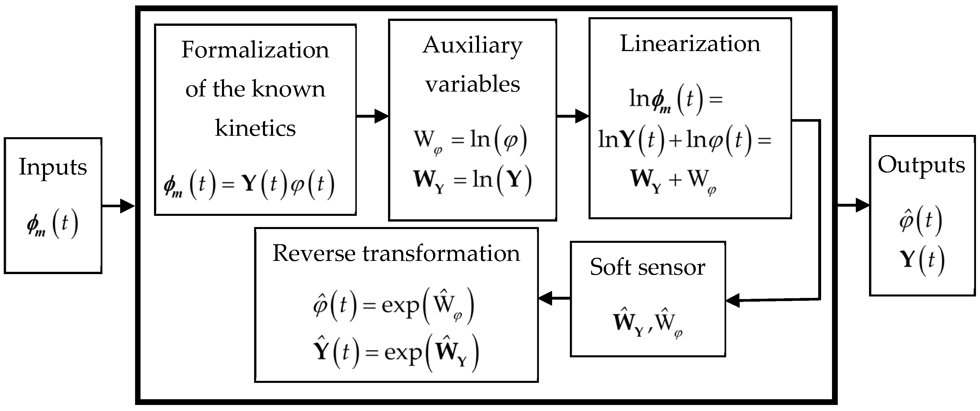
The general structure of software sensor Equations (7)–(9) is given in Figure 1. The inputs and kinetics formalization are presented by Equation (1). The auxiliary variables are calculated using Equations (2) and (3). Linearization is carried out according to Equations (4)–(6). The software sensor is described by system (7–9). The outputs are obtained by the reverse transformations using Equations (10) and (11).

The application of the original idea for the linearization of kinetics, by representing it in logarithmic form, leads to the derivation of a linear structure of the software sensor, system (7–9). This allowed us, by applying the well-known linear control theory, to study the stability of both SS structures (fourth- and fifth-order), as well as to reduce the number of SS’ design parameters to be tuned.

2.3. Stability Analysis

The following system of the estimation error dynamics is considered:

$$\frac{d\mathit{x}}{dt}=\mathbf{A}\mathit{x}+\mathit{u},$$

(12)

where

$\mathit{x}={\left[{\tilde{W}}_Y{\tilde{\mathrm{W}}}_{\phi }\tilde{p}\right]}^{\mathrm{T}}$, ${\tilde{W}}_Y=W_Y-{\widehat{W}}_Y$, ${\tilde{\mathrm{W}}}_{\phi }={\mathrm{W}}_{\phi }-{\widehat{\mathrm{W}}}_{\phi }$, $\tilde{p}=p-\widehat{p}$;

x—the estimation error vector with dim = 4 or 5; $W_Y$, ${\mathrm{W}}_{\phi }$, and p—‘true’ values of the parameters; ${\widehat{W}}_Y$, ${\widehat{\mathrm{W}}}_{\phi }$, and $\widehat{p}$—estimates of $W_Y$, ${\mathrm{W}}_{\phi }$, and p;

${\mathbf{A}}_{\left(m+2\right)\times \left(m+2\right)}=\left|\begin{array}{lll}-\mathsf{\omega }\hfill & -\mathit{\omega }\hfill & -1\hfill \\ -{\mathbf{\gamma }}^{\mathbf{{\rm T}}}\hfill & {\displaystyle \sum _{\gamma =1}^m-{\gamma }_i}\hfill & 1\hfill \\ -{\mathbf{\Psi }}^{\mathbf{{\rm T}}}\hfill & {\displaystyle \sum _{\mathbf{\Psi }=1}^m-{\psi }_i}\hfill & 0\hfill \end{array}\right|$, $\mathbf{\omega }=\left|\begin{array}{c}-{\omega }_1\\ -{\omega }_2\\ -{\omega }_3\\ \dots \\ -{\omega }_m\end{array}\right|$, $1={\left[\begin{array}{cccc}1& 1& \dots & 1\end{array}\right]}^{\mathrm{T}}$,

$\mathit{\omega }=\left|\begin{array}{cccc}-{\omega }_1& 0& 0& 0\\ 0& -{\omega }_2& 0& 0\\ 0& 0& \dots & 0\\ 0& 0& 0& -{\omega }_m\end{array}\right|$, ${\mathit{u}}_{\left(m+2\right)\times 1}={\left[0\dots 00\frac{dp}{dt}\right]}^{\mathrm{T}}$, where ω_i, γ_i, and ψ_i are the SS design parameters.

The concrete presentation of matrix A is:

$${\mathbf{A}}_{\left(m+2\right)\times \left(m+2\right)}=\left|\begin{array}{cccccc}-{\omega }_1& 0& 0& 0& -{\omega }_1& -1\\ 0& -{\omega }_2& 0& 0& -{\omega }_2& -1\\ 0& 0& \dots & 0& \dots & \dots \\ 0& 0& 0& -{\omega }_m& -{\omega }_m& -1_m\\ -{\gamma }_1& -{\gamma }_2& \dots & -{\gamma }_m& -{\gamma }_1-{\gamma }_2\dots -{\gamma }_m& 1\\ -{\psi }_1& -{\psi }_2& \dots & -{\psi }_m& -{\psi }_1-{\psi }_2\dots -{\psi }_m& 0\end{array}\right|.$$

(13)

The analysis of the observability shows that the system (7–9) (for m = 1, 2, and 3) was not completely observable, but detectable, which is equivalent to the existence of an asymptotically stable linear observer of the state [28]. Therefore, the parameter tuning of estimator (7–9) cannot guarantee exponential (arbitrarily chosen) convergence of estimates, but asymptotic convergence only.

The cases of m = 2 (fourth-order system) and m = 3 (fifth-order system) are considered below. In the case of m > 3, the polynomial degree of matrix A is greater than five, which leads to problems of the software sensor design [29].

2.3.1. Stability Analysis of the Fourth-Order System

The system stability is investigated based on the analysis of system (12), where matrix A and vectors x and u are presented as:

$$\mathbf{A}=\left|\begin{array}{llll}-{\omega }_1\hfill & 0\hfill & -{\omega }_1\hfill & -1\hfill \\ 0\hfill & -{\omega }_2\hfill & -{\omega }_2\hfill & -1\hfill \\ -{\gamma }_1\hfill & -{\gamma }_2\hfill & -{\gamma }_1-{\gamma }_2\hfill & 1\hfill \\ -{\gamma }_1-{\gamma }_2\hfill & -{\psi }_2\hfill & -{\psi }_1-{\psi }_2\hfill & 0\hfill \end{array}\right|;\mathit{x}={\left[{\tilde{\mathrm{W}}}_{y_1}{\tilde{\mathrm{W}}}_{y_2}{\tilde{\mathrm{W}}}_{\phi }\tilde{p}\right]}^{\mathrm{T}};\mathit{u}={\left[000\frac{dp}{dt}\right]}^{\mathrm{T}}.$$

(14)

The characteristic polynomial of matrix A is:

λ⁴ + λ³(ω₁ + ω₂ + γ₁ + γ₂) + λ²(ω₁ω₂ + (ω₁ + ω₂)(γ₁ + γ₂) − ψ₂ − γ₁ω₁) +
+ λ((ω₁ω₂ − ψ₂)(γ₁ + γ₂) − ψ₂ω₁ − γ₁ω₁ω₂) + ω₁γ₁ψ₂ − ω₂γ₂ψ₁ − ψ₂(γ₁ + γ₂)ω₁,

(15)

where λ is the variable of the characteristic polynomial.

If matrix A has four different Eigenvalues (λ₁ ÷ λ₄), the following system (including equalities and inequalities) has to be solved to guarantee the stability:

λ₁ + λ₂ + λ₃ + λ₄ = −ω₁ − ω₂ − γ₁ − γ₂ < 0,

(16)

λ₁λ₂ + λ₃λ₄ + (λ₁ + λ₂)(λ₃ + λ₄) = ω₁ω₂ + (ω₁ + ω₂)(γ₁ + γ₂) − ψ₂ − γ₁ω₁ > 0,

(17)

λ₃λ₄(λ₁+ λ₂) + λ₁λ₂(λ₃+ λ₄) = −(ω₁ω₂ − ψ₂)(γ₁ + γ₂) + ψ₂ω₁ + γ₁ω₁ω₂ < 0,

(18)

λ₁λ₂λ₃λ₄ = ω₁γ₁ψ₂ − ω₂γ₂ψ₁ − ψ₂(γ₁ + γ₂)ω₁ > 0.

(19)

Numerous variations of system (16-19) exist that lead to a solution of a system of four algebraic equations with four Eigenvalues and six tuning parameters.

2.3.2. Stability Analysis of the Fifth-Order System

Matrix A and vectors x and u are presented as follows:

$$\begin{array}{l}\mathbf{A}=\left|\begin{array}{lllll}-{\omega }_1\hfill & 0\hfill & 0\hfill & -{\omega }_1\hfill & -1\hfill \\ 0\hfill & -{\omega }_2\hfill & 0\hfill & -{\omega }_2\hfill & -1\hfill \\ 0\hfill & 0\hfill & -{\omega }_3\hfill & -{\omega }_3\hfill & -1\hfill \\ -{\gamma }_1\hfill & -{\gamma }_2\hfill & -{\gamma }_3\hfill & -{\gamma }_1-{\gamma }_2-{\gamma }_3\hfill & 1\hfill \\ -{\psi }_1\hfill & -{\psi }_2\hfill & -{\psi }_3\hfill & -{\psi }_1-{\psi }_2-{\psi }_3\hfill & 0\hfill \end{array}\right|;x={\left[{\tilde{\mathrm{W}}}_{y_1}{\tilde{\mathrm{W}}}_{y_2}{\tilde{\mathrm{W}}}_{y_3}{\tilde{\mathrm{W}}}_{\phi }\tilde{p}\right]}^{\mathrm{T}};\\ \mathit{u}={\left[0000\frac{dp}{dt}\right]}^{\mathrm{T}}.\end{array}$$

(20)

The characteristic polynomial of matrix A is:

λ⁵ + λ⁴(ω₁ + ω₂ + ω₃ + γ₁ + γ₂ + γ₃) + λ³(ω₁ω₂ + ω₁ω₃ + ω₂ω₃ +
(ω₁ + ω₂ + ω₃)(γ₁ + γ₂ + γ₃)) + λ²(ω₁ω₂ω₃ + (ω₂ω₃ + ω₁ω₂ + ω₁ω₃)(γ₁ + γ₂ + γ₃)) +
+ λ((ω₁ω₂ω₃)(γ₁+ γ₂+ γ₃) − ψ₁γ₂ω₂ − ψ₂γ₃ω₃) − ψ₁γ₂ω₂ω₃ − ψ₂γ₃ω₁ω_3.

(21)

In the case of the five different Eigenvalues λ₁ ÷ λ₅ of matrix A, the following system has to be solved to guarantee stability:

λ₁ + λ₂ + λ₃ + λ₄ + λ₅ = −ω₁ − ω₂ − ω₃ − γ₁ − γ₂ − γ₃ < 0,

(22)

λ₃λ₄ + λ₁λ₂ + (λ₁ + λ₂)(λ₃ + λ₄) + λ₅(λ₁ + λ₂ + λ₃ + λ₄) =
= ω₁ω₂ + ω₁ω₃ + ω₂ω₃ + (ω₁ + ω₂ + ω₃)(γ₁ + γ₂ + γ₃) > 0,

(23)

λ₃λ₄(λ₁ + λ₂) + λ₁λ₂(λ₃ + λ₄) + λ₃λ₄λ₅ + λ₁λ₂λ₅ + (λ₁ + λ₂)(λ₃ + λ₄)λ₅ =
= −ω₁ω₂ω₃ − (ω₂ω₃ + ω₁ω₂ + ω₁ω₃)(γ₁ + γ₂ + γ₃) < 0,

(24)

λ₁λ₂λ₃λ₄ + λ₃λ₄λ₅(λ₁ + λ₂) + λ₁λ₂λ₅(λ₃ + λ₄) =
ω₁ω₂ω₃(γ₁ + γ₂ + γ₃) − ψ₁γ₂ω₂ − ψ₂γ₃ω₃ > 0,

(25)

λ₁λ₂λ₃λ₄λ₅ = ψ₁γ₂ω₂ω₃ + ψ₂γ₃ω₃ω₁ < 0.

(26)

The general presentation of the fifth-order polynomial cannot be solved algebraically using finite number operations [29]. Many solutions of system (22–26) exist, presenting five algebraic equations with five Eigenvalues and nine tuning parameters. The parameter’s tuning could be different depending on the considered process and its dynamics, as it is shown in the example below.

3. Results and Discussion

3.1. Structure of the General Software Sensor

As a case study, a class of aerobic fed-batch processes carried out in homogenous conditions was considered. An operational model was derived. The model describes the dynamics of the key variables chosen from the expert’s point of view, as follows:

$$\frac{dX}{dt}={\varphi }_X\left(t\right)X-\frac{F}{V}X,$$

(27)

$$\frac{d{S}_1}{dt}=-{\varphi }_{S_1}\left(t\right)X+\frac{F}{V}{S}_{1m}-\frac{F}{V}{S}_1,$$

(28)

$$\frac{d{S}_2}{dt}=-{\varphi }_{S_2}\left(t\right)X-\frac{F}{V}{S}_2+Kla\left(C_{S_2}^{\ast }-S_2\right),$$

(29)

$$\frac{dRQ}{dt}=q_{RQ}\left(t\right),$$

(30)

$$\frac{dV}{dt}=F,$$

(31)

where X, S₁, S₂, and RQ are biomass, glucose, dissolved oxygen concentrations, and the respiratory quotient, respectively; F—glucose feed rate; V—culture volume; S_1m—glucose concentration in the feed; Kla—oxygen transfer coefficient; $C_{S_2}^{\ast }$—oxygen saturation concentration; ${\varphi }_X\left(t\right),{\varphi }_{S_1}\left(t\right),{\varphi }_{S_2}\left(t\right)$—rates of biomass growth, substrate consumption and dissolved oxygen consumption, respectively; $q_{RQ}\left(t\right)$—the change of the ration between the specific rates of carbon dioxide production and oxygen consumption $q_{C{O}_2}\left(t\right)/q_{S_2}\left(t\right)$.

In the considered case, a linear relationship exists between the experimental data of the specific oxygen consumption rate and the specific carbon dioxide producti on rate. This leads to problems in software sensor design. For this reason, the respiratory quotient RQ was used, as calculated from the on-line data of the off-gas analysis. As shown below, the relationship between the yield coefficient,$Y_{RQ/S_1}\left(t\right)$, related to RQ, and yield coefficients with biological meaning, $Y_{X/S_1}$ and Y_eth/pyr, is justified.

In practice, for the considered processes, on-line measurements of X, ${\varphi }_{S_2}\left(t\right)$, and RQ were available. Using the observer-based estimators published by the authors of [16], from on-line measurements of X and RQ, we received the rates ${\varphi }_X\left(t\right)$ and $q_{RQ}\left(t\right)$, which together with ${\varphi }_{S_2}\left(t\right)$, were accepted as inputs of the scheme from Figure 2.

Following the general formalization, each rate, ${\varphi }_X,{\varphi }_{S_2}$, and $q_{RQ}$, is presented as function of two terms considered as unknown time-varying parameters: The glucose consumption $\left({\varphi }_{S_1}\left(t\right)\right)$ as common term and a yield coefficient $\left(Y_{X/S_1}\left(t\right),Y_{S_2/S_1}\left(t\right),Y_{RQ/S_1}\left(t\right)\right)$, comprising the remaining parts of the corresponding kinetics:

$${\varphi }_X\left(t\right)={\varphi }_{S_1}\left(t\right)Y_{X/S_1}\left(t\right),$$

(32)

$${\varphi }_{S_2}\left(t\right)={\varphi }_{S_1}\left(t\right)Y_{S_2/S_1}\left(t\right),$$

(33)

$$q_{RQ}\left(t\right)={\varphi }_{S_1}\left(t\right)Y_{RQ/S_1}\left(t\right),$$

(34)

Equations (30) and (34) were derived assuming that the changes of the respiratory quotient can be expressed as:

$$\frac{dRQ}{dt}={\varphi }_{S_1}\left(t\right)\left(1-Y_{X/S_1}\right)k{Y}_{eth/pyr},$$

(35)

where Y_eth/pyr is the yield coefficient for ethanol production at the pyruvic acid branch point that is specific for the considered processes. Since the respiratory quotient RQ characterizes the degree of fermentative growth, it is postulated that its changes are proportional to the split of carbon toward ethanol synthesis at the pyruvic acid branch point under substrate limited conditions. Hence, the yield $Y_{RQ/S_1}\left(t\right)$ represent the term of Equation (34), including both ‘true’ yield coefficients, $Y_{X/S_1}$ and Y_eth/pyr, as follows:

$$Y_{RQ/S_1}\left(t\right)=\left(1-Y_{X/S_1}\right)k{Y}_{eth/pyr}.$$

(36)

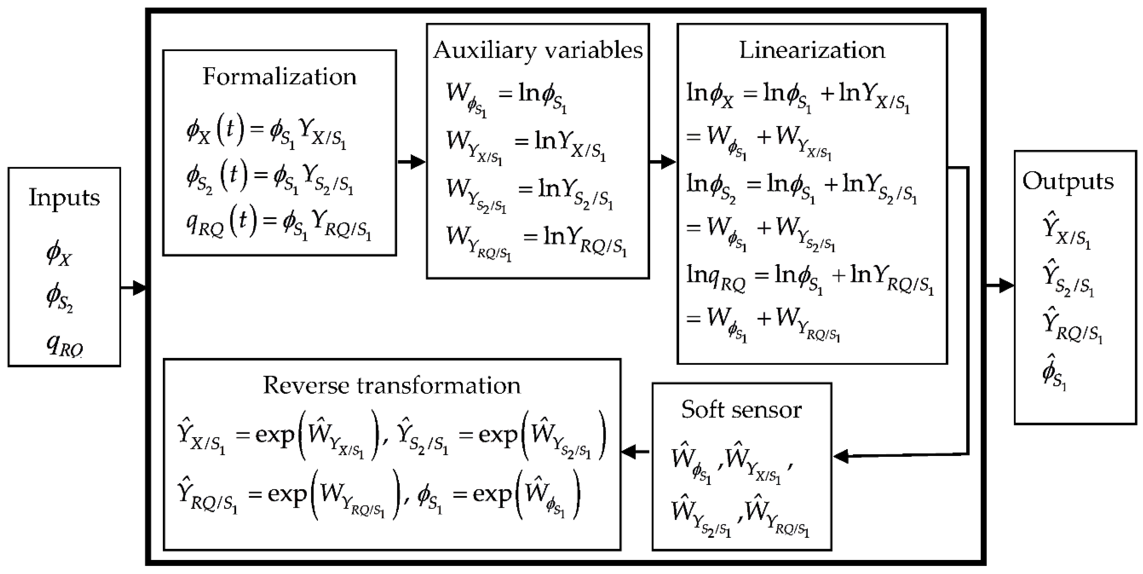
The monitoring of the kinetics of the processes described by system (32)–(36) was reduced to the estimation of four parameters—the yield coefficients $Y_{X/S_1}\left(t\right),Y_{S_2/S_1}\left(t\right),Y_{RQ/S_1}\left(t\right)$ and the glucose consumption rate ${\varphi }_{S_1}\left(t\right)$, which are outputs of the scheme shown in Figure 2. This figure repeats the structure of the general SS from Figure 1, where the information about each component corresponds to the considered case.

System (7–11), describing the general SS for the considered case, can be rewritten as follows:

$$\frac{d{\widehat{\mathrm{W}}}_{{\mathrm{Y}}_{X/S_1}}}{dt}=\frac{d{\varphi }_X}{{\varphi }_{X}dt}-\widehat{p}+{\omega }_1\left(\ln {\varphi }_X-{\widehat{\mathrm{W}}}_{{\varphi }_{S_1}}-{\widehat{\mathrm{W}}}_{{\mathrm{Y}}_{X/S_1}}\right),$$

(37)

$$\frac{d{\widehat{\mathrm{W}}}_{{\mathrm{Y}}_{S_2/S_1}}}{dt}=\frac{d{\varphi }_{S_2}}{{\varphi }_{S_2}dt}-\widehat{p}+{\omega }_2\left(\ln {\varphi }_{S_2}-{\widehat{\mathrm{W}}}_{{\varphi }_{S_1}}-{\widehat{\mathrm{W}}}_{{\mathrm{Y}}_{S_2/S_1}}\right),$$

(38)

$$\frac{d{\widehat{\mathrm{W}}}_{{\mathrm{Y}}_{RQ/S_1}}}{dt}=\frac{d{q}_{RQ}}{q_{RQ}dt}-\widehat{p}+{\omega }_3\left(\ln q_{RQ}-{\widehat{\mathrm{W}}}_{{\varphi }_{S_1}}-{\widehat{\mathrm{W}}}_{{\mathrm{Y}}_{RQ/S_1}}\right),$$

(39)

$$\frac{d{\widehat{\mathrm{W}}}_{{\varphi }_{S_1}}}{dt}=\widehat{p}+{\gamma }_1\left(\ln {\varphi }_X-{\widehat{\mathrm{W}}}_{{\varphi }_{S_1}}-{\widehat{\mathrm{W}}}_{{\mathrm{Y}}_{X/S_1}}\right)+{\gamma }_2\left(\ln {\varphi }_{S_2}-{\widehat{\mathrm{W}}}_{{\varphi }_{S_1}}-{\widehat{\mathrm{W}}}_{{\mathrm{Y}}_{S_2/S_1}}\right),$$

(40)

$$\frac{d\widehat{p}}{dt}={\psi }_1\left(\ln {\varphi }_X-{\widehat{\mathrm{W}}}_{{\varphi }_{S_1}}-{\widehat{\mathrm{W}}}_{{\mathrm{Y}}_{X/S_1}}\right).$$

(41)

This represents a fifth-order SS of the auxiliary variables ${\mathrm{W}}_{{\mathrm{Y}}_{X/S_1}}$, ${\mathrm{W}}_{{\mathrm{Y}}_{S_2/S_1}}$, ${\mathrm{W}}_{{\mathrm{Y}}_{RQ/S_1}}$, ${\mathrm{W}}_{{\varphi }_{S_1}}$. The values of ${\varphi }_X$ and $q_{RQ}$, as well as their time-derivatives at the right side of Equations (37) and (39), were obtained as explained above. The time-derivatives of ${\varphi }_{S_{2m}}$ in (38) were calculated by numerical differentiation.

The outputs of the SS,${\mathrm{Y}}_{X/S_1}\left(t\right),{\mathrm{Y}}_{S_2/S_1}\left(t\right),{\mathrm{Y}}_{RQ/S_1}\left(t\right)$, and ${\varphi }_{S_1}\left(t\right)$, are obtained by the reverse functions:

$${\widehat{\mathrm{Y}}}_{X/S_1}=\exp \left({\widehat{\mathrm{W}}}_{{\mathrm{Y}}_{X/S_1}}\right),$$

(42)

$${\widehat{\mathrm{Y}}}_{S_2/S_1}=\exp \left({\widehat{\mathrm{W}}}_{{\mathrm{Y}}_{S_2/S_1}}\right),$$

(43)

$${\widehat{\mathrm{Y}}}_{RQ/S_1}=\exp \left({\widehat{\mathrm{W}}}_{{\mathrm{Y}}_{RQ/S_1}}\right),$$

(44)

$${\widehat{\varphi }}_{S_1}=\exp \left({\widehat{\mathrm{W}}}_{{\varphi }_{S_1}}\right).$$

(45)

3.2. Tuning Procedure

The structure of the derived software sensor systems (37)–(45) was simplified in comparison to the general structure (7)–(11). An optimal dimension of vectors γ and Ψ was proposed with the aim to facilitate the tuning procedure. It was based on stability analysis of the system’s error.

Taking into account the dynamics of processes in homogenous conditions, it is accepted that:

λ₁= λ₂= λ₃= λ₄= λ₅= λ.

(46)

The value of λ can be obtained by an optimization procedure (minimization of the square of sum of estimation errors) using experimental data of each of the investigated processes of the class described by system (27)–(31):

$$\mathrm{sum}\left(e^2\right)={\tilde{\varphi }}_X^2+{\tilde{\varphi }}_{S_2}^2+{\tilde{q}}_{RQ}^2\to \min ,$$

(47)

where

$${\tilde{\varphi }}_X\left(t\right)={\widehat{\varphi }}_X\left(t\right)-{\widehat{\varphi }}_{S_1}\left(t\right){\widehat{\mathbf{Y}}}_{X/S_1}\left(t\right),$$

(48)

$${\tilde{\varphi }}_{S_2}\left(t\right)={\varphi }_{S_{2m}}\left(t\right)-{\widehat{\varphi }}_{S_1}\left(t\right){\widehat{\mathbf{Y}}}_{S_2/S_1}\left(t\right),$$

(49)

$${\tilde{q}}_{RQ}\left(t\right)={\widehat{q}}_{RQ}\left(t\right)-{\widehat{\varphi }}_{S_1}\left(t\right){\widehat{\mathbf{Y}}}_{RQ/S_1}\left(t\right),$$

(50)

${\widehat{\varphi }}_X\left(t\right)$ and ${\widehat{q}}_{RQ}\left(t\right)$ are estimates of ${\varphi }_X$ and $q_{RQ}$, obtained similarly to [16]. Estimates ${\widehat{\mathbf{Y}}}_{X/S_1}\left(t\right),{\widehat{\mathbf{Y}}}_{S_2/S_1}\left(t\right),{\widehat{\mathbf{Y}}}_{RQ/S_1}\left(t\right)$, and ${\widehat{\varphi }}_{S_1}\left(t\right)$ were received by the system (37)–(45).

The calculation of the design parameters is based on the following stability conditions:

5λ = −ω₁ − ω₂ − ω₃ < 0,

(51)

10λ² = ω₂ω₃ + ω₁(ω₂ + ω₃) > 0,

(52)

10λ³ = −ω₁ω₂ω₃ < 0,

(53)

5λ⁴ = −ω₂γ₂ψ₁ > 0,

(54)

λ⁵ = ω₂ω₃γ₂ψ₁ < 0.

(55)

Based on (54) and (55), the following relation between the design parameter ω₃ and the Eigenvalue is obtained:

ω₃ = −λ/3 > 0.

(56)

The following auxiliary parameters D, B, and C are introduced:

5λ = D < 0,

(57)

10λ² = B > 0,

(58)

10λ³ = C < 0.

(59)

Substituting the terms ω₂ω₃ and (ω₂ + ω₃) from (52) with their equivalents from the Equations (53) and (51), respectively, the following third order polynomial of parameter ω₁ is derived:

$${\omega }_1^3+\mathbf{D}{\omega }_1^2+\mathbf{B}{\omega }_1+\mathbf{C}=0.$$

(60)

One of the roots of (60) is denoted as:

$${\omega }_1=\sqrt[3]{-\frac{q}{2}+\sqrt{Q}}+\sqrt[3]{-\frac{q}{2}-\sqrt{Q}}-\frac{A}{3},$$

(61)

where q = −2(D/3)³ − DB/3 + C, Q = (α/3)³ + (q/2)², α = D²/3 + B.

The design parameter ω₂ is calculated from (51):

ω₂ = −ω₁ − ω₃ − D.

(62)

The values of the parameters ω₃ and ω₁ are obtained from Equation (56) and Equation (61), respectively.

The value of the parameter γ₂ is calculated from (55) by:

γ₂ = λ⁵/ω₂ω₃ψ₁.

(63)

To satisfy the stability condition (55), the value of ψ₁ has to be negative. For the parameter γ₁, we assumed the relationship γ₁ = γ₂ > 0.

Realizing the steps from Equation (51) to Equation (63), the values of all tuning parameters were received. The proposed tuning procedure reduced the SS design to choose of one tuning parameter only.

A fed-batch cultivation process of B. subtilis, carried out in the laboratory bioreactor, was considered as being representative. Two experiments (Experiment I and Experiment II), carried out in STR, were used for the demonstration of theoretical results [30].

The calculation of the specific oxygen uptake rate (q_S2m) and carbon dioxide production rate (q_CO2m) was performed on the basis of a gas balance of the input and output flow using O₂ and CO₂ measurements in the off-gas. The specific oxygen uptake rate, cell dry weight, and respiratory quotient RQ = q_CO2m/q_S2m were available as on-line measurements, which were used in the calculation of the SS inputs.

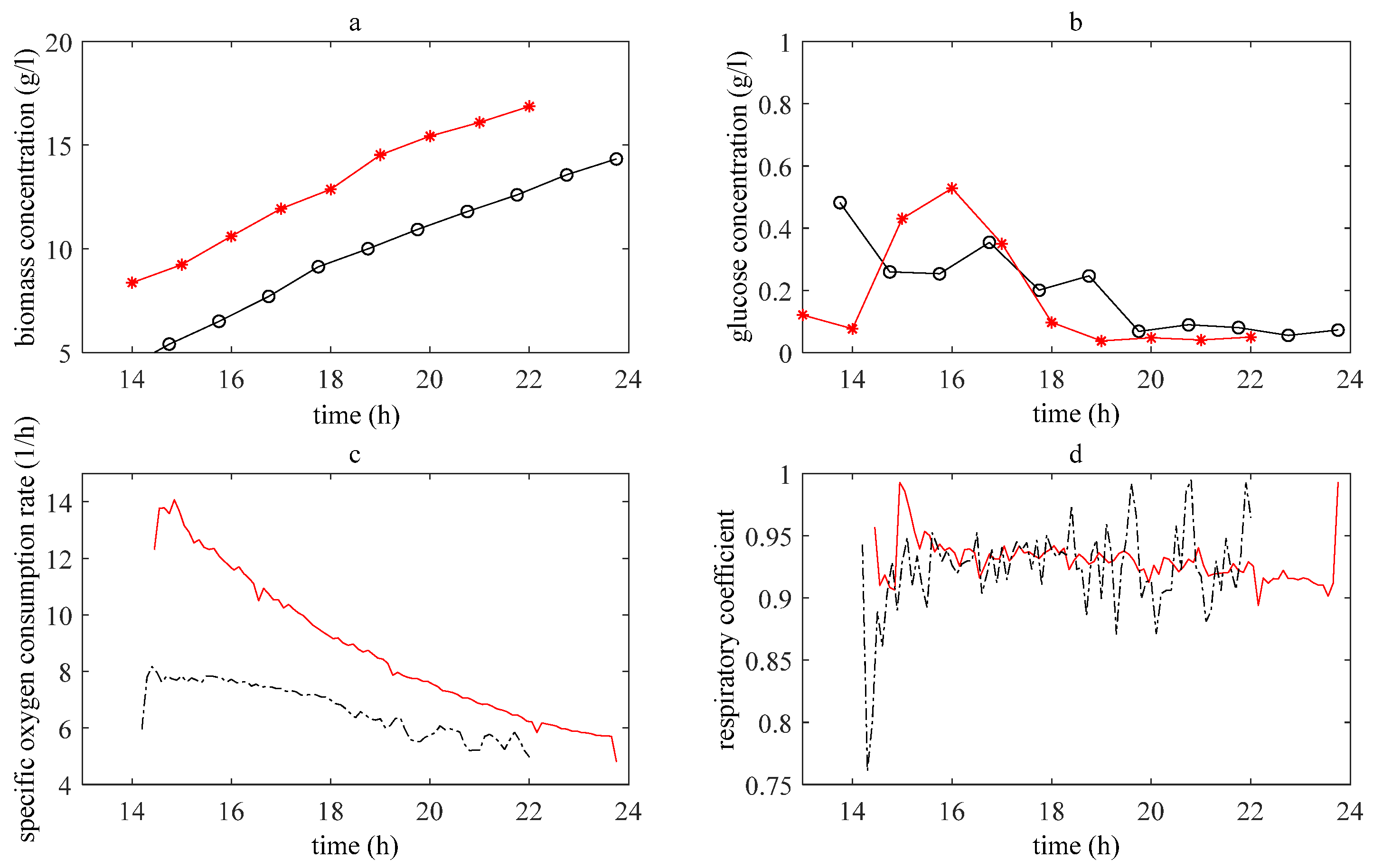
The two sets of experimental data are shown in Figure 3. On-line measurements are shown in Figure 3a,c,d. In Figure 3b, off-line measurements of glucose concentration are shown. Both experiments were performed under the same conditions, but as it can be seen, they varied due to a lack of reproducibility of experiments. In order to demonstrate adaptive performance of the proposed SS shown in Figure 2, the tuning of software sensors was conducted using the data of Experiment I, while the data of the Experiment II were used for validation.

For investigations, a program package was prepared in a MATLAB environment (MATLAB R2019a, the MathWorks, Inc., Natick, MA, USA, 2019). The package included software sensor systems (37)–(45) and both sets of experimental data from Figure 3. The value λ = −42, used in the tuning procedure, was obtained based on the optimization procedure with the criteria given in Equations (47)–(50).

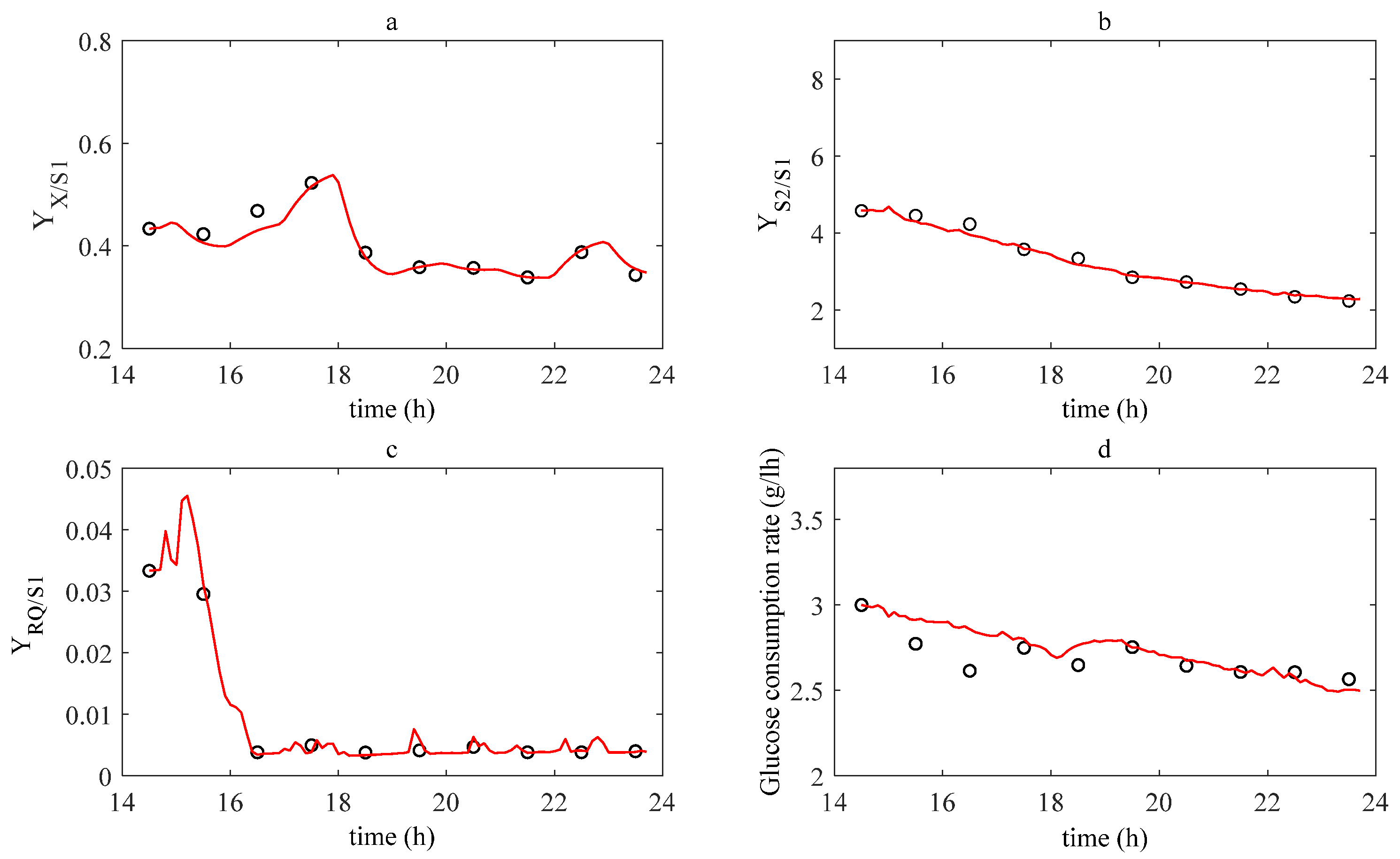
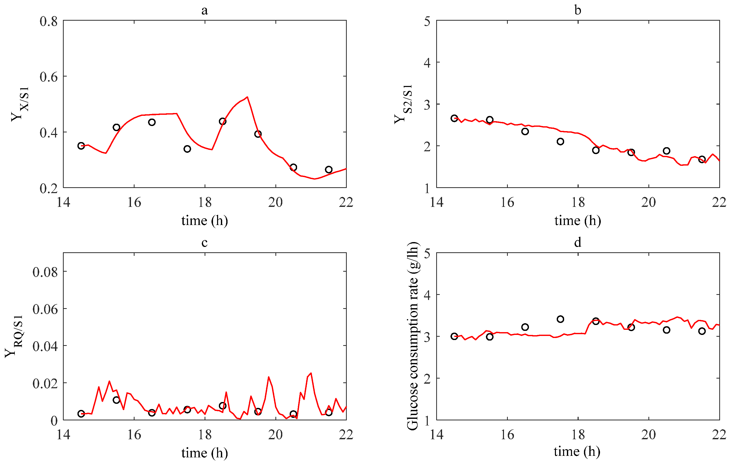
Estimates of $Y_{X/S_1}\left(t\right),Y_{S_2/S_1}\left(t\right),Y_{RQ/S_1}\left(t\right)$, and ${\varphi }_{S_1}\left(t\right)$ are shown in Figure 4 and Figure 5. The estimation results under the Experiment I are shown in Figure 4. The verification results are presented in Figure 5. To show the accuracy of the outputs, their reference values were derived using laboratory measurements of glucose concentration, S₁. A discrete observer-based estimator allowed us to obtain discrete estimates of glucose consumption rate, $R_{S_{-}ref}={\varphi }_{S_1{}_{-}ref}$, for both experiments. The reference values of $Y_{X/S_1}\left(t\right),Y_{S_2/S_1}\left(t\right),Y_{RQ/S_1}\left(t\right)$ were calculated using relationships (32)–(34) and ${\varphi }_{S_1{}_{-}ref}$. All reference values are shown in Figure 4 and Figure 5 with points.

As it can be seen from the results in Figure 4 and Figure 5, the dynamics of the yield coefficients and the substrate consumption rate had different profiles for the two experiments, although the experiments were realized under homogeneous conditions. This can be explained with the dynamic nature of bioprocesses and fluctuations in the strain performance. Comparing the two experiments, the values of the yield coefficients retained the trend of change to some extent, while the rate of consumption of the substrate slightly decreased in Experiment 1 (Figure 4d), but stayed more or less constant in Experiment 2 (Figure 5d).

The results, shown in Figure 4 and Figure 5, demonstrate the good performance and adaptive properties of the proposed SS. As can be expected, the accuracy of the estimation and their convergence were better for the experiment used for the tuning of the estimator. The estimates converged to the corresponding reference values with a mean relative error below 3%.

The simulations proved the reliability of the proposed methodology for real-time assessment. By setting only one design parameter, a good accuracy of the estimates of each term of the kinetics with a clear physical meaning was achieved. By verifying with data from another experiment, the adaptability of the proposed approach was demonstrated.

4. Conclusions

In this paper, a general approach for kinetics monitoring of a class of biotechnological processes was proposed. This class of processes is characterized by a relationship between measured and estimated parameters that guarantees the synthesis of asymptotically stable SS.

The originality of this approach consists of its (i) presentation of the process kinetics with two unknown time-varying parameters with clear physical meaning, (ii) derivation of a linear structure of the SS using logarithmic transformations of these parameters that facilitate stability analysis, and (iii) derivation of stable fourth- and fifth-order structures of the SS, satisfying conditions for asymptotical stability.

The proposed approach was applied for the monitoring of process kinetics realized in homogeneous conditions. The tuning procedure was reduced to one design parameter, which led to an automatic calculation of the others. The adaptability of the proposed method was proven by its application to two B. subtilis fed-batch cultivations. The tuning of the SS was realized with one set of experimental data, and its validation was demonstrated by the other dataset. The accuracy of the obtained estimates is good enough for monitoring of the process dynamics and can be applied for process investigations and control design.

In comparison to our previous investigations, the presented methodology provides the possibility to reduce the tuning procedure to only one tuning parameter.

The obtained results are a good basis to extend both the theoretical investigations and their applications in the future. One of the possible directions of research is the integration of physiological parameters that can be measured on-line. This will expand the applicability of the presented approach, as there is a strong relationship between yield coefficient dynamics and the physiological state of cells.

References

- Hausmann, R.; Henkel, M.; Hecker, F.; Hitzmann, B. Present Status of Automation for Industrial Bioprocesses. In Current Developments in Biotechnology and Bioengineering; Larroche, C., Sanromán, M.Á., Du, G., Pandey, A., Eds.; Elsevier: Amsterdam, The Netherlands, 2017; pp. 725–757. [Google Scholar]
- Pörtner, R.; Barradas, O.P.; Frahm, B.; Hass, V.C. Advanced process and control strategies for bioreactors. In Current Developments in Biotechnology and Bioengineering; Larroche, C., Sanromán, M.Á., Du, G., Pandey, A., Eds.; Elsevier: Amsterdam, The Netherlands, 2017; pp. 463–493. [Google Scholar]
- Assis, A.; Filho, R.M. A new approach for designing model-based indirect sensors. Comp. Chem. Eng. 2000, 24, 1099–1103. [Google Scholar]
- Bastin, G.; Dochain, D. On-Line Estimation and Adaptive Control of Bioreactors; Elsevier: Amsterdam, The Netherlands, 1990. [Google Scholar]
- Soons, Z.; Voogt, J.A.; van Straten, G.; van Boxtel, A.J.B. Constant specific growth rate in fed-batch cultivation of Bordetella pertussis using adaptive control. J. Biotechnol. 2006, 125, 252–268. [Google Scholar] [CrossRef] [PubMed]
- Veloso, A.; Rocha, I.; Ferreira, E.C. Monitoring of fed-batch E. coli fermentations with software sensors. Bioprocess. Biosys. Eng. 2009, 32, 381–388. [Google Scholar] [CrossRef] [Green Version]
- Gonzalez, K.; Tebbani, S.; Lopes, F.; Thorigné, A.; Givry, S.; Dumur, D.; Pareau, D. Feedback linearizing controller coupled to an unscented Kalman filter for lactic acid regulation. In Proceedings of the IEEE 19th International Conference on System Theory, Control and Computing (ICSTCC), Cheile Gradistei, Romania, 14–16 October 2015; pp. 219–224. [Google Scholar]
- Hadj-Abdelkader, O.; Hadj-Abdelkader, A. Estimation of substrate and biomass concentrations in a chemostat using an extended Kalman filter. Int. J. Bioautomation 2019, 23, 215–232. [Google Scholar] [CrossRef]
- Valdés-González, H.; Flaus, J.M.; Acuña, G. Moving horizon state estimation with global convergence using interval techniques: Application to biotechnological processes. J. Proc. Contr. 2003, 13, 325–336. [Google Scholar] [CrossRef]
- Cruz-Bournazou, M.N.; Barz, T.; Nickel, D.; Glauche, F.; Knepper, A.; Neubauer, P. Online optimal experimental re-design in robotic parallel fed-batch cultivation facilities for validation of macro-kinetic growth models at the example of E. coli. Biotechnol. Bioengin. 2017, 114, 610–619. [Google Scholar] [CrossRef] [PubMed]
- Georgieva, P.; de Azevedo, S.F. Novel computational methods for modeling and control in chemical and biochemical process systems. In Computational Intelligence Techniques for Bioprocess Modelling, Supervision and Control; Nicoletti, M., Lakhmi, C.J., Eds.; Springer: Berlin/Heidelberg, Germany, 2009; pp. 99–125. [Google Scholar]
- Selişteanu, D.; Petre, E.; Roman, M.; Şendrescu, D. Estimation of kinetic rates in a baker’s yeast fed-batch bioprocess by using non-linear observers. IET Control. Theory A 2012, 6, 243–253. [Google Scholar] [CrossRef] [Green Version]
- Lyubenova, V.; Ignatova, M.; Salonen, K.; Kiviharju, K.; Eerikäinen, T. Control of α-amylase production by Bacillus subtilis. Bioproc. Biosyst. Eng. 2011, 34, 367–374. [Google Scholar] [CrossRef]
- Nuñez, S.; Garelli, F.; De Battista, H. Product-based sliding mode observer for biomass and growth rate estimation in Luedeking-Piret like processes. Chem. Eng. Res. Des. 2016, 105, 24–30. [Google Scholar] [CrossRef]
- Battista, H.; Picó, J.; Garelli, F.; Navarro, J.L. Reaction rate reconstruction from biomass concentration measurement in bioreactors using modified second-order sliding mode algorithms. Bioproc. Biosyst. Eng. 2012, 35, 1615–1625. [Google Scholar] [CrossRef]
- Petre, E.; Selişteanu, D.; Roman, M. Nonlinear robust adaptive control strategies for a lactic fermentation process. J. Chem. Technol. Biot. 2018, 93, 518–526. [Google Scholar] [CrossRef]
- Hajji, M.; Rapaport, A. Design of a cascade observer for a model of bacterial batch culture with nutrient recycling. In Biomass Now—Cultivation and Utilization; Matovic, M.D., Ed.; InTech Open: London, UK, 2013; pp. 97–112. [Google Scholar]
- Lyubenova, V.; Ignatova, M. Cascade software sensors for monitoring of activated sludge wastewater treatment processes. Compt. Rend. Acad. Bulg. Sci. 2011, 64, 395–404. [Google Scholar]
- Zlatkova, A.; Lyubenova, V. Dynamics monitoring of fed-batch E. coli fermentation. Int. J. Bioautomation 2017, 21, 121–132. [Google Scholar]
- Bezzaoucha, S.; Marx, B.; Maquin, D.; Ragot, J. Nonlinear joint state and parameter estimation: Application to a wastewater treatment plant. Contr. Eng. Pract. 2013, 21, 1377–1385. [Google Scholar] [CrossRef] [Green Version]
- Patarinska, T.; Trenev, V.; Popova, S. Software sensors design for a class of aerobic fermentation processes. Int. J. Bioautomation 2010, 14, 99–118. [Google Scholar]
- Lyubenova, V.; Junne, S.; Ignatova, M.; Neubauer, P. Software sensor design considering oscillating conditions as present in industrial scale fed-batch cultivations. Biotech. Bioeng. 2013, 110, 1945–1955. [Google Scholar] [CrossRef]
- Lemoine, A.; Delvigne, F.; Bockisch, A.; Neubauer, P.; Junne, S. Tools for the determination of population heterogeneity caused by inhomogeneous cultivation conditions. J. Biotechnol. 2017, 251, 84–93. [Google Scholar] [CrossRef]
- Delvigne, F.; Zacchetti, B.; Fickers, P.; Fifani, B.; Roulling, F.; Lefebvre, C.; Neubauer, P.; Junne, S. Improving controllability of microbial cell factories: From single cell to large-scale bioproduction. FEMS Microbiol. Lett. 2018, 365. [Google Scholar] [CrossRef]
- Lin, H.Y.; Mathiszik, B.; Xu, B.; Enfors, S.O.; Neubauer, P. Determination of the maximum specific uptake capacities for glucose and oxygen in glucose limited fed-batch cultivations of Escherichia coli. Biotechnol. Bioeng. 2001, 73, 347–357. [Google Scholar] [CrossRef]
- Neubauer, P.; Lin, H.Y.; Mathiszik, B. Metabolic load of recombinant protein production: Inhibition of cellular capacities for glucose uptake and respiration after induction of heterologous genes in Escherichia coli. Biotechnol. Bioeng. 2003, 83, 53–64. [Google Scholar] [CrossRef]
- Lubenova, V. Stable adaptive algorithm for simultaneous estimation of time-varying parameters and state variables in aerobic bioprocesses. Biopr. Eng. 1999, 21, 219–226. [Google Scholar] [CrossRef]
- Damm, T.; Ethington, C. Detectability, observability, and asymptotic reconstructability of positive systems. Lect. Notes Control. Inf. Sci. 2009, 389, 63–70. [Google Scholar]
- Birkhoff, G.; Mac Lane, S. A Survey of Modern Algebra, 5th ed.; Macmillan: New York, NY, USA, 1996; pp. 418–421. [Google Scholar]
- Junne, S.; Klingner, A.; Kabisch, J.; Schweder, T.; Neubauer, P. A two-compartment bioreactor system made of commercial parts for bioprocess scale-down studies: Impact of oscillations on Bacillus subtilis fed-batch cultivations. Biotech. J. 2011, 6, 1009–1017. [Google Scholar] [CrossRef] [PubMed]
Figure 1.
General structure of kinetics software sensor.
Figure 2.
Software sensor scheme for the considered case.
Figure 3.
Inputs of software sensor: (a): biomass concentration, (b): glucose concentration, (c): specific oxygen consumption rate, (d): respiratory coefficient. Experiment I measurements (red lines); Experiment II measurements (black lines).
Figure 4.
Tuning using Experiment I measurements: Comparison between experimental data (points) and estimates (red lines): (a): yield coefficient ; (b): yield coefficient ; (c): yield coefficient ; (d): glucose consumption rate.
Figure 5.
Verification using Experiment II measurements: Comparison between experimental data (points) and estimates (red lines). (a): yield coefficient ; (b): yield coefficient ; (c): yield coefficient ; (d): glucose consumption rate.
Publisher’s Note: MDPI stays neutral with regard to jurisdictional claims in published maps and institutional affiliations. |
© 2020 by the authors. Licensee MDPI, Basel, Switzerland. This article is an open access article distributed under the terms and conditions of the Creative Commons Attribution (CC BY) license (http://creativecommons.org/licenses/by/4.0/).
Share and Cite
MDPI and ACS Style
Lyubenova, V.; Ignatova, M.; Roeva, O.; Junne, S.; Neubauer, P. Adaptive Monitoring of Biotechnological Processes Kinetics. Processes 2020, 8, 1307. https://0-doi-org.brum.beds.ac.uk/10.3390/pr8101307
AMA Style
Lyubenova V, Ignatova M, Roeva O, Junne S, Neubauer P. Adaptive Monitoring of Biotechnological Processes Kinetics. Processes. 2020; 8(10):1307. https://0-doi-org.brum.beds.ac.uk/10.3390/pr8101307
Chicago/Turabian StyleLyubenova, Velislava, Maya Ignatova, Olympia Roeva, Stefan Junne, and Peter Neubauer. 2020. "Adaptive Monitoring of Biotechnological Processes Kinetics" Processes 8, no. 10: 1307. https://0-doi-org.brum.beds.ac.uk/10.3390/pr8101307
Note that from the first issue of 2016, this journal uses article numbers instead of page numbers. See further details here.