Prediction of the Solubility of CO₂ in Imidazolium Ionic Liquids Based on Selective Ensemble Modeling Method

Abstract

Solubility data is one of the essential basic data for CO₂ capture by ionic liquids. A selective ensemble modeling method, proposed to overcome the shortcomings of current methods, was developed and applied to the prediction of the solubility of CO₂ in imidazolium ionic liquids. Firstly, multiple different sub–models were established based on the diversities of data, structural, and parameter design philosophy. Secondly, the fuzzy C–means algorithm was used to cluster the sub–models, and the collinearity detection method was adopted to eliminate the sub–models with high collinearity. Finally, the information entropy method integrated the sub–models into the selective ensemble model. The validation of the CO₂ solubility predictions against experimental data showed that the proposed ensemble model had better performance than its previous alternative, because more effective information was extracted from different angles, and the diversity and accuracy among the sub–models were fully integrated. This work not only provided an effective modeling method for the prediction of the solubility of CO₂ in ionic liquids, but also provided an effective method for the discrimination of ionic liquids for CO₂ capture.

1. Introduction

With the increase of energy consumption in industrial production, reducing CO₂ emissions and increasing CO₂ absorption have become an essential means to alleviate environmental degradation [1]. Room–temperature ionic liquids, which are relatively new compounds, have gained much attention in recent years, and had the potential to be considered as an alternative to conventional volatile organic solvents in the reaction and separation processes. Information about the solubility and the rate of solubility is a crucial factor for consideration of ionic liquids in potential industrial processes [2,3]. A large number of ionic liquids can be synthesized due to their special ionic structure. Due to some difficulties associated with experimental measurements and the cost of ionic liquids, it is more advantageous to develop predictive methods for prediction of the phase behavior of such systems [4,5,6]. Therefore, the modeling prediction methods have become an important way to obtain the solubility data of CO₂ in ionic liquids, which is divided into the mechanism modeling method and the data–driven modeling method.

In order to understand and predict the phase behavior of CO₂ and ionic liquid mixtures, Perturbed Hard Sphere Chain Equation of State (PHSC) has been selected to simulate the CO₂ absorption in a series of ionic liquids [7]. CO₂ solubility in ionic liquids had been calculated based on two thermodynamic models, namely the UNIQUAC model and the quantum model, based on COSMO–RS theory of interacting molecular surface charge [8]. Venkatramanet et al. [9] used molecular descriptors based on quantum chemistry computations to predict the solubility of CO₂ in different ionic liquids. Although the mechanism modeling method has the advantage of strong model interpretability, thermodynamic model is relatively complex and requires complicated mathematical operations [10]. Considering the complex parameters of mechanism model, a multi–model fusion method was proposed to predict the solubility of CO₂ in ionic liquids [11].

Based on the radial basis function artificial neural network (RBFANN) and least squares support vector machine (LSSVM) combined with group contribution (GC) method, RBFANN–GC and LSSVM–GC were used to study the model of CO₂ absorption in polyionic liquids [12]. Four different methods based on artificial intelligence were proposed to predict CO₂ solubility in different ionic liquids [13]: the predictive capability of the Least Square Support Vector Machine (LSSVM), Adaptive Neuro–Fuzzy Inference System (ANFIS), Multi–Layer Perceptron Artificial Neural Network (MLP–ANN), and Radial Basis Function Artificial Neural Network (RBF–ANN) have been evaluated for estimating carbon dioxide solubility in 67 different ionic liquids [14]. The Classification And Regression Tree (CART) methodology in modeling CO₂ solubility in different ionic liquids is also under investigation [15]. Artificial neural networks (ANNs) technique was proposed as a new approach to predict the solubility of CO₂ in ethanol–[EMIM][Tf2N] ionic liquid mixtures [16]. Although the data–driven models have the advantage of high prediction accuracy, they are mainly based on the single models, which have shortcomings such as easy to fall into local optimality and cannot describe the global characteristics of the problem. As a result, the prediction performance of any of these models is limited.

A selective ensemble method based on data–driven model is proposed in this paper for the deficiency of the current mechanism model method and data–driven model method. Firstly, on the premise of ensuring the accuracy and diversity of the ensemble, fuzzy C–means and collinearity detection algorithms were used to eliminate redundant models. Then the sub–models with different predictive capabilities were integrated by using the information entropy method, so as to fully mine the performance of various models, realize the full coverage of information describing the problem and improve the prediction accuracy of the model. Finally, the method was applied to predict the solubility of CO₂ in ionic liquids and to evaluate its prediction performance.

2. Methods

2.1. Sub–Model Training

Zhou et al. [17] proposed the theory of ‘many can be better than all’, which presupposed that the sub–models had a high degree of diversity and accuracy. The diversity of sub–models had an essential impact on improving the generalized performance of ensemble models [18,19]. The sub–models were established based on data, structural, and parameter diversities.

2.1.1. Data Diversity

Multiple datasets from the original dataset were generated based on data diversity to train different sub–models. The data sets should be different from each other to obtain different results from the trained sub–models. Bootstrap aggregation (Bagging), Adaptive Boosting (AdaBoost), and random subspace were commonly used to achieve data diversity. To generate several training sets with different attributes, the bootstrap algorithm was introduced to achieve the goal. When re–sampling was enough, about 36.8% of the given data sets did not appear in the constructed training set, which ensured the diversity of the data.

2.1.2. Structural Diversity

Different model structures were used to induce structural diversity, and three data–driven algorithms (Back Propagation Neural Network (BPNN), Extreme Learning Machine (ELM), and Radial Basis Function Neural Network (RBFNN)) were used to train the generated sub–training sets. These sub–models varied in size and architecture, and such collections were called heterogeneous ensemble [20]. To control the diversity in the heterogeneous integration, the ‘overproduce and choose’ strategy was performed. Firstly, a large number of models were trained; then, a selection or combination of these models was made to optimize performance, which purpose was to minimize the size of the ensemble model without significantly reducing the accuracy of the model [21,22].

2.1.3. Parameter Diversity

Parameter diversity uses different parameter sets to generate different sub–models. Even if the same training set is used, the output of the sub–model may vary with different parameter sets. The method of adjusting the internal parameters of the model was adopted to ensure the diversity of model parameters. For BPNN and ELM, the internal parameters of the adjusted model are the number of neurons, the activation function and the number of hidden layers. For RBFNN, the internal parameters of the adjusted model are the kernel function center and width.

2.2. Sub–Model Discrimination

To improve the prediction ability of the ensemble model or reduce the prediction cost, it is necessary to screen the established sub–models and avoid multicollinearity in the sub–model as much as possible. As one of the main techniques of unsupervised machine learning, fuzzy clustering analysis had been widely used in large–scale data analysis, data mining, pattern recognition, and other fields [23,24,25]. The fuzzy C–means clustering was used to screen the sub–model in this study.

N sub–models are defined, the parameters of each model are w_i (I = 1,2,…,N), c sub–models are clustered centers and denoted by m_j (j = 1,2,…,c), the sample set is S = {(x¹,y₁),(x²,y₂),…,(xⁿ,y_n)}, where x is the input variable, y is the output variable, and n is the number of data in the sample set. For all the sub–models to be clustered, the difference between the models can be measured by the Euclidean distance between the sub–models. The calculation formula of the Euclidean distance is as follow:

$$D\left(w_i,m_j\right)={\displaystyle \sum _{k}d\left(y\left(w_i,x^k\right),y\left(m_j,x^k\right)\right)}$$

(1)

where $d\left(r_1,r_2\right)={\Vert r_1-r_2\Vert }_2$ is the distance between the sub–models, and $y\left(w_i,x^k\right)$ and $y\left(m_j,x^k\right)$ represent the output of $x^k$ on the parameters w_i and m_j, respectively. The results of the sub–models on the input data set were adopted to define the difference between the models. The larger the Euclidean distance was, the greater the difference between the two sub–models was.

To perform cluster analysis on the sub–models, the outputs of each sub–model on the sample point x_k (k = 1,2,…,n) is composed into a vector, namely: z_i = (y(w_i,x¹),y(w_i,x²),…,y(w_i,xⁿ)) (I = 1,2,…,N), the outputs of N sub–models with dimension n can be obtained. To determine the optimal number of clusters output by the N sub–models, CH indicators and Davies—Bouldin (DB) could be used as evaluation indicators. In consideration of computational efficiency, the CH evaluation index was utilized to determine the optimal number of clusters. The CH index used the intra–class dispersion matrix to describe the tightness and the inter–class dispersion matrix to describe the separation. The specific calculation formula is as follow:

$$\mathrm{CH}\left(k\right)=\frac{trB\left(k\right)/\left(k-1\right)}{trW\left(k\right)/\left(n-k\right)}$$

(2)

where n is the number of clusters, k is the current class, trB(k) is the trace of the inter–class dispersion matrix, and trW(k) is the trace of the intra–class dispersion matrix. The larger the CH is, the closer and the more disperse the class is. When the number of clusters is 1, the CH evaluation index cannot be used.

In the clustering process, when the difference between the two sub–models is very large, it means that the two sub–models are likely to be in different clusters, otherwise they may be in the same cluster. Due to the similarity of the sub–models in the same cluster, the output results obtained by these sub–models under the same input are similar [26]. When the fuzzy C–means algorithm is applied to over–generated sub–models, it is necessary to detect the collinearity of the sub–models in each cluster [27]. Belsleyet et al. [28] believed that the existence of collinearity between models will not only increase the workload of modeling, but also affect the actual performance of the model. The variance expansion coefficient (VIF) was used to judge the collinearity of each sub–model. The larger the value of VIF was, the more serious the collinearity was. 10 are taken as the judgment boundary: when VIF < 10, there is no multicollinearity; when 10 ≤ VIF ≤ 100, there is strong multicollinearity; when VIF ≥ 100, there is serious multicollinearity. The calculation formula of VIF is as follows:

$$\mathrm{VIF}=\frac{1}{1-R^2{}_i}$$

(3)

where R_i represents the multiple determination coefficient of the independent variable x_i for the regression analysis of other independent variables.

2.3. Sub–Model Ensemble

The weight coefficient of the sub–model generally reflects the degree of influence of the sub–model on the ensemble model. The reasonable determination of the weight coefficients of the sub–models will directly affect the prediction accuracy of the model, so it is necessary to adopt appropriate methods to determine the weight coefficients of each sub–model. Information entropy is an effective measurement tool to describe information content (information structure, uncertainty, etc.). Using the information entropy method to determine the weight coefficient of each sub–model can effectively reduce the impact of the weak sub–model on the model performance [29]. In this paper, the information entropy method is used to obtain the weight coefficient of the optimal sub–model [11].

2.4. Implementation Step

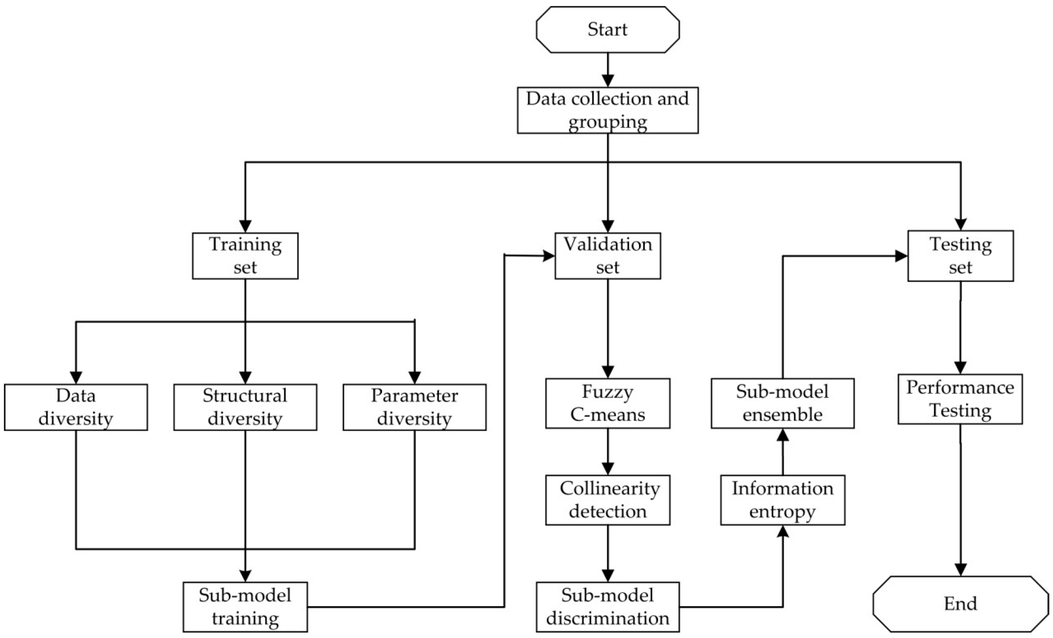
A new selective ensemble modeling method was established, and its implementation process is shown in Figure 1, which mainly includes data collection and grouping, sub–model training, sub–model discrimination, and sub–model ensemble and model performance testing. The specific implementation steps were as follows:

(1) Data collection and grouping

The appropriate auxiliary variables were determined as the input variables of the model, and the dominant variable to be predicted were taken as the output variable of the model. Firstly, the collected original samples data set was normalized, and then the preprocessed original sample data set was randomly divided into a training set, a validation set, and a test set in an appropriate ratio. The training set was ensured to cover all the types of the experimental data and operating conditions.

(2) Sub–model training

Firstly, different training sets were generated based on the diversity of the data. Then, multiple BPNN sub–models, ELM sub–models, and RBFNN sub–models with different structural parameters were established by using the realization method of structure diversity and parameter diversity, so that these sub–models have the characteristics of high diversity and accuracy.

(3) Sub–model discrimination

The validation set was used to evaluate the predictive performance of all sub–models, and the Euclidean distance was used as the standard to evaluate the differences of sub–models. The fuzzy C–means algorithm was adopted to cluster all the sub–models, and the Calinski–Harabasz (CH) method was used to determine the optimal cluster number. After clustering, the collinearity detection method was used to eliminate some sub–models with high collinearity in the same cluster, and only some of the sub–models without collinearity were retained.

(4) Sub–model ensemble and model performance testing

The information entropy method was utilized to calculate the weight coefficients of the retained sub–models, so as to establish the selective ensemble model. Then the test set was used to evaluate the prediction performance of the model.

3. Results and Discussion

3.1. Data Collecting and Grouping

Six essential parameters, including temperature, pressure, critical temperature (Tc), critical pressure (Pc), molecular weight (MW), and eccentricity factor (w) were taken as input variables for the CO₂ solubility predictive models [30,31]. Temperature and pressure will affect the solubility of CO₂ in the ionic liquid. For the same ionic liquid, the solubility of CO₂ in the ionic liquid increases when the temperature decreases or the pressure increases. Theoretically, Tc, Pc, M and w are the essential thermodynamic properties of ionic liquids. They can distinguish the species of ionic liquids and reflect the characteristics of ionic liquid structures [13,31]. In addition, the input variables of the model were only applicable to imidazolium ionic liquids. The solubility of CO₂ in ionic liquids was selected as the output variable of the model.

Data of critical temperature (Tc), critical pressure (Pc), molecular weight (M) and eccentricity factor (w) of nine imidazolium ionic liquids were collected by referring to a large number of literatures, as shown in

Table 1. Critical parameters of imidazolium ionic liquids.

NO.	Ionic Liquids	MW (g/mol)	Tc (K)	Pc (MPa)	w
1	[BMIM][BF4]	226.03	623.30	2.040	0.8489
2	[EMIM][TF2N]	391.30	788.05	3.310	1.2250
3	[EMIM][ETSO4]	236.29	1061.10	4.040	0.3368
4	[HMIM][TF2N]	447.92	1292.78	2.389	0.3893
5	[HMIM][TFO]	316.34	1055.60	2.495	0.4890
6	[HMIM][BF4]	254.08	716.61	1.794	0.6589
7	[HMIM][MESO4]	278.37	1110.84	2.961	0.4899
8	[BMMIM][TF2N]	433.40	1255.80	2.031	0.3193
9	[HMIM][PF6]	312.24	759.16	1.550	0.9385

[7,32,33,34,35,36,37,38,39,40,41]. The name and abbreviation of imidazolium ionic liquid are shown in

Table 2. Name and abbreviation of imidazolium ionic liquid.

NO.	Abbreviation	Name
1	[BMIM][BF4]	1–butyl–3–methylimidazolium tetrafluoroborate
2	[EMIM][TF2N]	1–ethyl–3–methylimidazolium bis(trifluoromethylsulfonyl)imide
3	[EMIM][ETSO4]	1–ethyl–3–methylimidazolium ethylsulfate
4	[HMIM][TF2N]	1–hexyl–3–methylimidazoliumbis(trifluoromethylsulfonyl)imide
5	[HMIM][TFO]	1–hexyl–3–methylimidazolium trifluoromethanesulfonate
6	[HMIM][BF4]	1–hexyl–3–methylimidazolium tetrafluoroborate
7	[HMIM][MESO4]	1–hexyl–3–methylimidazolium methyl–sulfate
8	[BMMIM][TF2N]	1–butyl–2,3–dimethylimidazoliumbis(trifluoromethanesulfonyl)imide
9	[HMIM][PF6]	1–methyl–3–hexylimidazolium hexafluorophosphate

. Meanwhile, a large number of data on the solubility of CO₂ in the nine imidazolium ionic liquids were collected, as shown in

Table 3. Solubility data of CO₂ in different imidazolium ionic liquids.

NO.	Ionic Liquids	Temperature Range (K)	Pressure Range (MPa)	CO2 Solubility Range (Mole Fraction)	NO. of Samples	Refs.
1	[BMIM][BF4]	278.47–368.22	0.01–67.62	0.003–0.610	204	[8,32,41]
2	[EMIM][TF2N]	450.49–292.75	0.00–43.25	0.000–0.782	250	[32,35,37,38,41]
3	[EMIM][ETSO4]	398.04–353.15	0.10–9.46	0.000–0.457	82	[39,40]
4	[HMIM][TF2N]	278.12–450.49	0.01–45.28	0.001–0.824	394	[8,33,38]
5	[HMIM][TFO]	303.15–373.15	1.25–100.12	0.267–0.816	34	[33]
6	[HMIM][BF4]	293.18–373.15	0.31–86.60	0.071–0.703	160	[8,33,37,39]
7	[HMIM][MESO4]	303.15–373.15	0.87–50.14	0.158–0.602	48	[33,39]
8	[BMMIM][TF2N]	298.15–343.15	0.01–1.90	0.002–0.211	36	[8,37]
9	[HMIM][PF6]	298.15–373.15	0.30–94.60	0.058–0.727	160	[8,34,36]

. A total of 1468 sets of samples were collected. All the solubility of CO₂ in ionic liquids in this paper was obtained in the equilibrium phase. The unit of the stoichiometry of reagents gas/ionic liquids is the molar ratio. For all sample data of each type of ionic liquid, 80% (1176 sets) were randomly selected as the training set for training the sub–model, 10% (146 sets) were randomly selected as the validation set for sub–model discrimination and sub–model ensemble, and the remaining 10% (146 sets) was used as the test set for the performance test of the ensemble model.

3.2. Selective Ensemble Model Developing

3.2.1. Sub–Model Training

In order to ensure the diversity of the data, the re–sampling technique (bootstrap) was used to generate 30 sub–training sets. In order to ensure the diversity of the sub–model structure and parameters, BPNN, ELM, and RBFNN were used to divide the generated 30 training sets randomly to these three algorithms, and 30 sub–models were obtained. All sub–models were implemented by MATLAB software (version 2016a, MathWorks, Natick, MA, USA). The structure and parameters of BPNN, ELM, and RBFNN sub–models were as follows:

(1) BPNN

Ten sub–models of BP neural network were established with a single hidden layer structure. The transfer function of the hidden layer was a tansig type excitation function, and the output layer was expanded by a purelin–type excitation function for range expansion. The training termination error was 4 × 10⁻⁴, and the learning rate was 0.05. The Levenberg–Marquardt algorithm was used in the training algorithm and the number of hidden layer nodes was 6–15.

(2) ELM

Ten sub–models were established by adjusting the number of hidden layers and activation functions of the extreme learning machine. There were 5 sub–models with sigmoid activation function (the number of hidden layer nodes was 113–117), and 5 sub–models with sin activation function (the number of hidden layer nodes was 115–119).

(3) RBFNN

Ten sub–models were established by adjusting the number of neurons and the activation function. Among them, the activation function used Gaussian kernel function, the center selection of the basis function adopted K–means clustering, the learning rate was 0.1, the training termination error was 1 × 10⁻⁴, and the number of neurons was 71–80.

3.2.2. Sub–Model Discrimination

The performance of the 30 sub–models established was evaluated by the validation set. Firstly, the fuzzy C–means algorithm was adopted to cluster all the sub–models, and then, the sub–models with high collinearity were eliminated based on the collinearity detection program. The performance indexes used for model evaluation included the mean absolute error (MAE), root mean square error (RMSE), and correlation coefficient (R²). The specific calculation formula for each index was as follows:

$$MAE=\frac{1}{N}{\displaystyle \sum _{i=1}^N\left|x_i-{\widehat{x}}_i\right|}$$

(4)

$$RMSE=\sqrt{\frac{{\displaystyle \sum _{i=1}^N{\left({\widehat{x}}_i-x_i\right)}^2}}{N}}$$

(5)

$$R^2=1-\frac{{\displaystyle \sum _{i=1}^N{\left({\widehat{x}}_i-x_i\right)}^2}}{{\displaystyle \sum _{i=1}^N{\left({\widehat{x}}_i-\overline{x}\right)}^2}}$$

(6)

where N was the number of samples, x_i was the predicted value of the sample i, ${\widehat{x}}_i$ was the true value of the sample i, and $\overline{x}$ was the average of all samples.

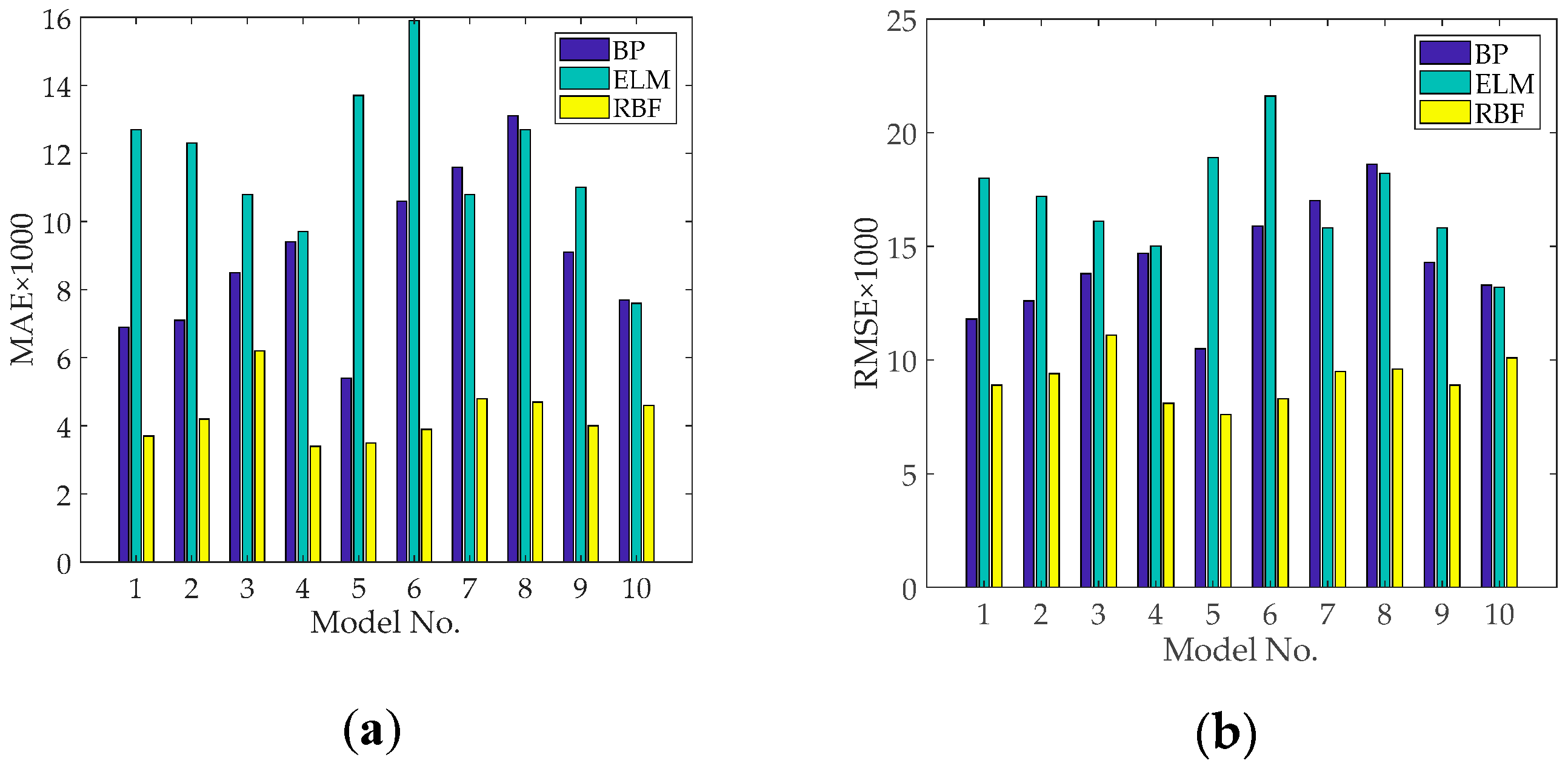
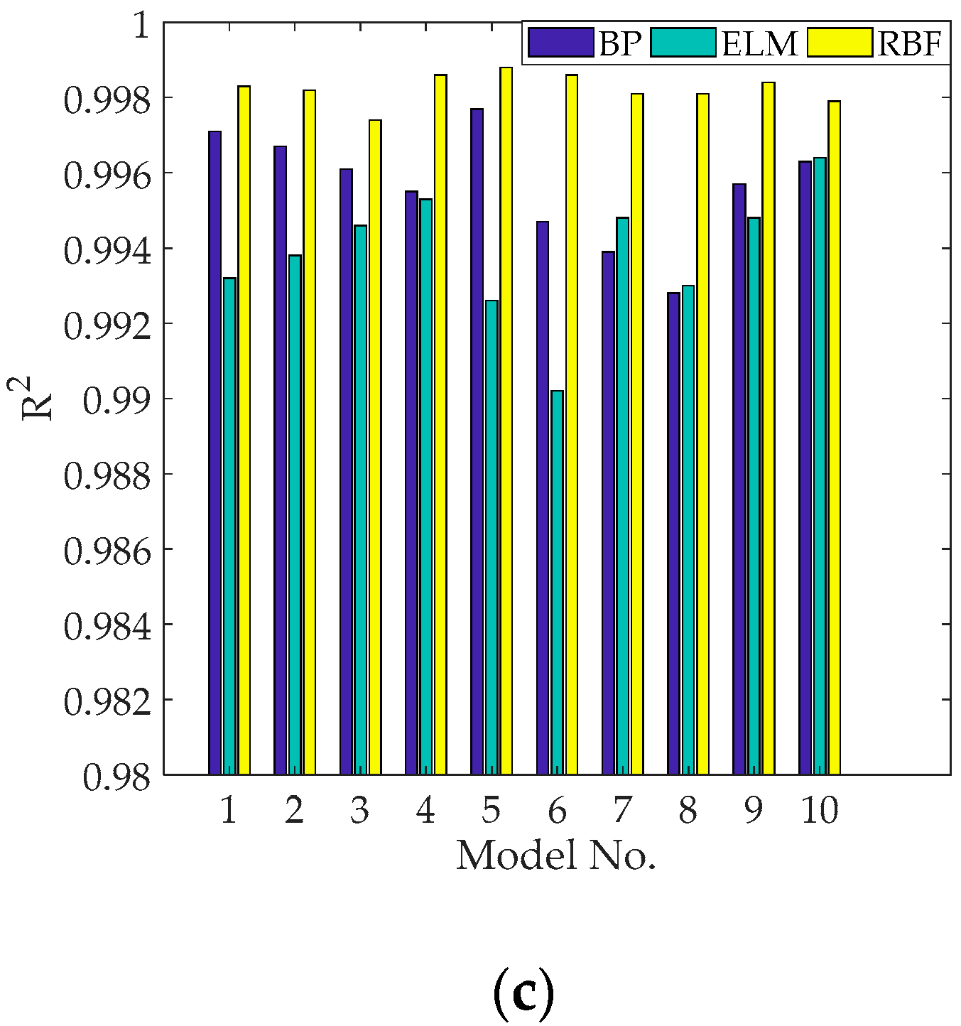
The performance index data of each sub–model was obtained from the validation set. The performance index data of the BPNN, ELM, and RBFNN sub–models are shown in

Table 4. Performance index data of back propagation neural network (BPNN) sub–models (Validation set).

NO.	MAE	RMSE	R2
1	0.0069	0.0118	0.9971
2	0.0071	0.0126	0.9967
3	0.0085	0.0138	0.9961
4	0.0094	0.0147	0.9955
5	0.0054	0.0105	0.9977
6	0.0106	0.0159	0.9947
7	0.0116	0.0170	0.9939
8	0.0131	0.0186	0.9928
9	0.0091	0.0143	0.9957
10	0.0077	0.0133	0.9963

,

Table 5. Performance index data of extreme learning machine (ELM) sub–models (Validation set).

NO.	MAE	RMSE	R2
1	0.0127	0.0180	0.9932
2	0.0123	0.0172	0.9938
3	0.0108	0.0161	0.9946
4	0.0097	0.0150	0.9953
5	0.0137	0.0189	0.9926
6	0.0159	0.0216	0.9902
7	0.0108	0.0158	0.9948
8	0.0127	0.0182	0.9930
9	0.0110	0.0158	0.9948
10	0.0076	0.0132	0.9964

and

Table 6. Performance index data of radial basis function neural network (RBFNN) sub–models (Validation set).

NO.	MAE	RMSE	R2
1	0.0037	0.0089	0.9983
2	0.0042	0.0094	0.9982
3	0.0062	0.0111	0.9974
4	0.0034	0.0081	0.9986
5	0.0035	0.0076	0.9988
6	0.0039	0.0083	0.9986
7	0.0048	0.0095	0.9981
8	0.0047	0.0096	0.9981
9	0.0040	0.0089	0.9984
10	0.0046	0.0101	0.9979

and Figure 2, respectively. It can be seen from Table 4, Table 5 and Table 6 that all BPNN, ELM, and RBFNN sub–models had good model performance.

The fuzzy C–means algorithm was used to cluster all the sub–models in Table 4, Table 5 and Table 6, and the CH index was used as the standard to evaluate the number of clusters. Formula (2) was applied to calculate the value of CH. The specific results are shown in

Table 7. Calinski–Harabasz (CH) value.

NO. of Cluster	CH Value
2	17.25
3	21.44
4	15.22
5	12.61

. It can be seen from Table 7 that when the number of clusters was 3, the value of CH reaches the maximum; thus, the number of clusters was selected as 3. When three classes were selected as clustering target, the following clustering results could be obtained: the first class included seven sub–models (5 BPNN sub–models and 2 ELM sub–models), the second class included 12 sub–models (10 RBFNN sub–models and 2 BPNN sub–models), and the third class included 11 sub–models (3 BPNN sub–models and 8 ELM sub–models).

Since the sub–models might be collinearity after clustering, it is necessary to carry out collinearity detection on the sub–models in the cluster to eliminate the adverse effects of collinearity. Variance Inflation Factor (VIF) was applied to judge the collinearity. The criterion was that there was no collinearity when VIF < 10. According to the criterion, the following results were obtained: 3 BPNN sub–models in the first class, 3 RBFNN sub–models in the second class, 2 BPNN sub–models, and 1 ELM sub–model in the third class.

3.2.3. Sub–Model Ensemble

For the nine sub–models obtained by discrimination, the information entropy method was used to calculate the weight coefficient of each sub–model. The specific results were as follows:

$$\begin{array}{l}Y=0.1130y_{11}+0.0898y_{12}+0.0875y_{13}+0.1755y_{21}+0.1545y_{22}\\ \begin{array}{cc}& \end{array}+0.1633y_{23}+0.0763y_{31}+0.0713y_{32}+0.0688y_{33}\end{array}$$

(7)

where Y is the output of the selective ensemble model based on information entropy, y_ij (i = 1,2,3, j = 1,2,3) is each sub–model, where i is the number of clusters, and j is the number of sub–models in the clustering number.

3.3. Model Performance Testing

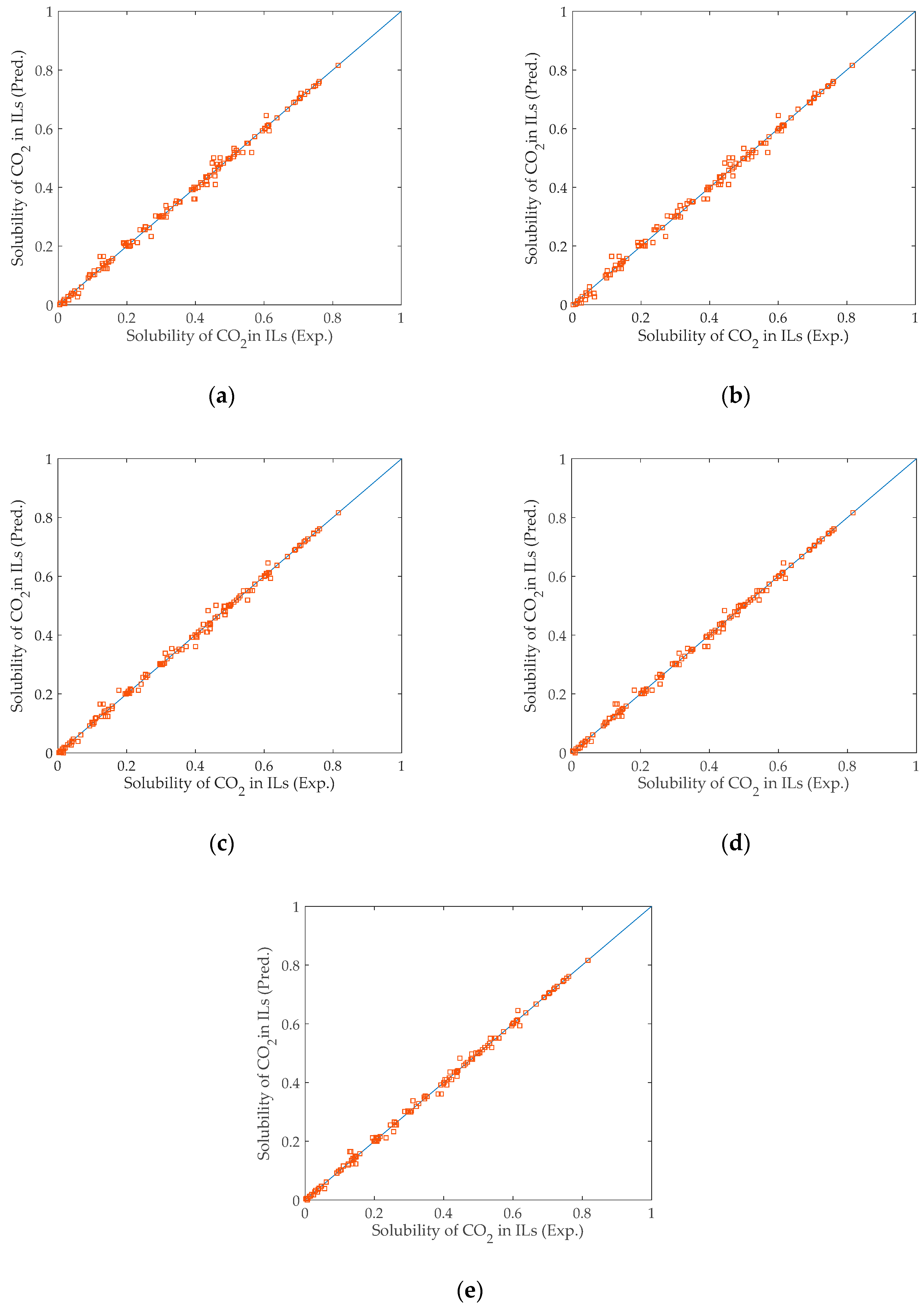
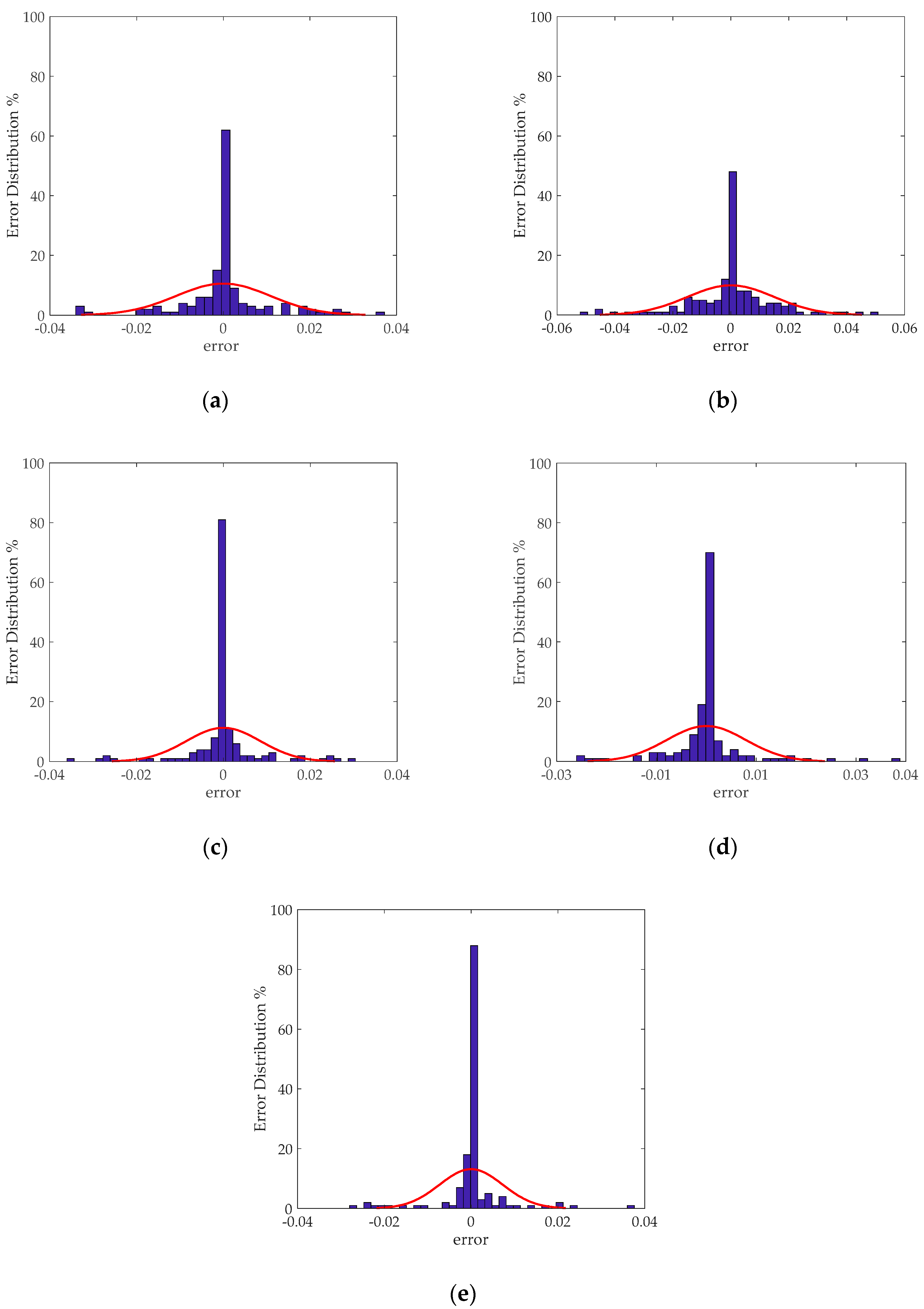
In order to compare the predictive performance of the selective ensemble model based on information entropy (selective ensemble model), the optimal BPNN sub–model (optimal BPNN), the optimal ELM sub–model (optimal ELM), the optimal RBFNN sub–model (optimal RBFNN), and the fully integrated model based on information entropy (fully integrated model) were also established. The test set was used to conduct performance tests on all the above models. The prediction performance of each model is shown in Figure 3. As shown in Figure 3, all models can well realize the prediction of the solubility of CO₂ in imidazolium ionic liquids. The histograms of the error distributions of the models are shown in Figure 4. Compared with the single optimal sub–model and the fully integrated model, from the perspective of error distribution, the selective ensemble model had smaller errors, which also verified the effectiveness of the proposed model. In other words, Figure 4 also proved the superiority of the selective ensemble model.

In order to quantitatively compare the prediction performance of the five models,

Table 8. Prediction performance data of five models (Testing set).

Model	MAE	RMSE	R2
Optimal BPNN	0.0082	0.0137	0.9960
Optimal ELM	0.0094	0.0150	0.9952
Optimal RBFNN	0.0066	0.0118	0.9971
Fully integrated model	0.0055	0.0103	0.9978
Selective ensemble model	0.0049	0.0096	0.9981

gave the specific results of MAE, RMSE, and R² of the five models based on the testing set.

It can be seen from Table 8 that all models have good prediction performance due to the reasonable selection of relevant physical and chemical parameters and structural parameters as the input of the prediction model for the solubility of CO₂ in ionic liquids.

Compared with the three optimal sub–models, the fully integrated model and the selective ensemble model made full use of the advantages of data diversity, parameter diversity, and structural diversity. The sub–models with different structures could excavate more global information contained in the data, and extract the useful information from the data by their different operation mechanisms. Both ensemble models were effective in reducing the error from predictions, thus improving the overall predictive performance. In addition, the information entropy method was used to reasonably select the combination weight coefficients of each sub–model. The models with different predictive abilities were assigned to different weight coefficients. In addition, the differences among the sub–models were fully considered, so that the prediction performance of the model was further improved.

Compared with the fully integrated model based on information entropy, the selective ensemble model based on information entropy used the fuzzy C–means algorithm and the collinearity detection method to screen the sub–models, which further ensured the diversity and accuracy of the models in different clusters, and removed the interference of some sub–models, thus ensuring the effectiveness of the selective ensemble model. Simultaneously, the selective ensemble model based on information entropy further fully mined the information inside the model, and extracted the useful information in the data from different angles to a great extent, and further improved the overall predictive performance.

4. Conclusions

In this paper, a selective ensemble modeling method for predicting the solubility of CO₂ in imidazolium ionic liquids was proposed. The implementation process of the selective ensemble modeling method included sub–model training, sub–model discrimination, sub–model ensemble and model performance testing. Sub–model training made full use of the advantages of data diversity, structural diversity, and parameter diversity. Sub–model discrimination used a fuzzy C–means clustering algorithm and collinearity detection method to ensure model diversity and reduce model collinearity. Sub–model ensemble adopted the information entropy weighting method to effectively reduce the impact of weak sub–models on model performance. The result of the prediction performance on the solubility of CO₂ in imidazolium ionic liquids showed that the solubility prediction model established by the selective ensemble modeling method had the best prediction performance compared with the other four models.

Although the prediction model established by the fusion modeling method had a good prediction effect for nine imidazolium ionic liquids in this study, it may not be applicable to predicting the solubility of CO₂ in other ionic liquids. The research work not only provides a feasible method to obtain the solubility data of CO₂ in ionic liquids, but also provides an effective means for further discrimination of ionic liquids, which has important practical significance.

References

- Xu, M.M.; Wang, S.J. Research progress of liquid–liquid phase variable solvent trapping CO2 technology. Chinese J. Chem. Eng. 2018, 69, 1809–1818. [Google Scholar]
- Taimoor, A.A.; Al–Shahrani, S.; Muhammad, A. Ionic liquid (1–butyl–3–metylimidazolium methane sulphonate) corrosion and energy analysis for high pressure CO2 absorption process. Processes 2018, 6, 45. [Google Scholar] [CrossRef] [Green Version]
- Leonzio, G.; Zondervan, E. Surface–response analysis for the optimization of a carbon dioxide absorption process using [hmim][Tf2N]. Processes 2020, 8, 1063. [Google Scholar] [CrossRef]
- Rogers, R.D. Chemistry: Ionic liquids–solvents of the future? Science. 2003, 302, 792–793. [Google Scholar] [CrossRef]
- Ding, J.; Xiong, Y.; Yu, D.H. Solubility of CO2 in ionic liquids–measuring and modeling methods. Chem. Ind. Eng. Prog. 2012, 31, 732–741. [Google Scholar]
- Bahmani, A.R.; Sabzi, F.; Bahmani, M. Prediction of solubility of sulfur dioxide in ionic liquids using artificial neural network. J. Mol. Liq. 2015, 211, 395–400. [Google Scholar] [CrossRef]
- Bazargani, Z.; Sabzi, F. Thermodynamic modeling of CO2 absorption in 1–butyl–3–methylimidazolium–based ionic liquids. J. Mol. Liq. 2016, 223, 235–242. [Google Scholar] [CrossRef]
- Kamgar, A.; Rahimpour, M.R. Prediction of CO2 solubility in ionic liquids with QM and UNIQUAC models. J. Mol. Liq. 2016, 222, 195–200. [Google Scholar] [CrossRef]
- Venkatraman, V.; Alsberg, B.K. Krakenx: Software for the generation of alignment–independent 3D descriptors. J. Mol. Mode. 2016, 22, 92–100. [Google Scholar] [CrossRef]
- Bavoh, C.B.; Lal, B.; Nashed, O.; Khan, M.S.; Keong, L.K.; Bustam, M.A. COSMO–RS: An ionic liquid prescreening tool for gas hydrate mitigation. Chinese J. Chem. Eng. 2016, 24, 1619–1624. [Google Scholar] [CrossRef]
- Xia, L.Y.; Wang, J.C.; Liu, S.S.; Li, Z.; Pan, H.T. Prediction of CO2 solubility in ionic liquids based on multi–model fusion method. Processes 2019, 7, 258. [Google Scholar] [CrossRef] [Green Version]
- Kardani, M.N.; Baghban, A.; Sasanipour, J.; Mohammadi, A.H.; Habibzadeh, S. Group contribution methods for estimating CO2 absorption capacities of imidazolium and ammonium–based polyionic liquids. J. Clean. Prod. 2018, 203, 601–618. [Google Scholar] [CrossRef]
- Tatar, A.; Naseri, S.; Bahadori, M.; Hezave, A.Z.; Kashiwao, T.; Bahadori, A.; Darvish, H. Prediction of carbon dioxide solubility in ionic liquids using MLP and radial basis function (RBF) neural networks. J. Taiwan. Inst. Chem. E. 2015, 60, 151–164. [Google Scholar] [CrossRef]
- Alireza, B.; Amir, H.M.; Mohammad, S.T. Rigorous modeling of CO2 equilibrium absorption in ionic liquids. Int. J. Greenh. Gas. Con. 2017, 58, 19–41. [Google Scholar]
- Ghiasi, M.M.; Mohammadi, A.H. Application of decision tree learning in modelling CO2 equilibrium absorption in ionic liquids. J. Mol. Liq. 2017, 242, 594–605. [Google Scholar] [CrossRef]
- Mirarab, M.; Sharifi, M.; Ghayyem, M.A.; Mirarab, F. Prediction of solubility of CO2 in ethanol–[EMIM][Tf2N] ionic liquid mixtures using artificial neural networks based on genetic algorithm. Fluid. Phase. Equilibr. 2014, 371, 6–14. [Google Scholar] [CrossRef]
- Zhou, Z.H.; Wu, J.; Wei, T. Ensembling neural networks: Many could be better than all. Artif. Intell. 2002, 137, 239–263. [Google Scholar] [CrossRef] [Green Version]
- MendesMoreira, J.; Soares, C.; Jorge, A.M.; De Sousa, J.F. Ensemble approaches for regression: A survey. Acm. Comput. Surv. 2012, 45, 11–40. [Google Scholar]
- Zhu, P.F.; Xia, L.Y.; Pan, H.T. Multi–model fusion modeling method based on improved kalman filter algorithm. Chinese J. Chem. Eng. 2015, 66, 1388–1394. [Google Scholar]
- Ren, Y.; Zhang, L.; Suganthan, P.N. Ensemble classification and regression–recent developments, applications and future directions. IEEE. Comput. Intell. M. 2016, 11, 41–53. [Google Scholar] [CrossRef]
- Sagi, O.; Rokach, L. Ensemble learning: A survey. Wires. Data. Min. Knowl. 2018, 8, 1249–1266. [Google Scholar] [CrossRef]
- Martínez–Muoz, G.; HernándezLobato, D.; Suárez, A. An analysis of ensemble pruning techniques based on ordered aggregation. IEEE T. Pattern. Anal. 2009, 31, 245–259. [Google Scholar] [CrossRef] [PubMed] [Green Version]
- Mojarad, M.; Nejatian, S.; Parvin, H.; Mohammadpoor, M. A fuzzy clustering ensemble based on cluster clustering and iterative fusion of base clusters. Appl. Intell. 2019, 49, 2567–2581. [Google Scholar] [CrossRef]
- Bowen, F.; Yun, F.Q.; Wan, J.L. Fuzzy clustering ensemble model based on distance decision. Chin. J. Electron. 2018, 54, 823–831. [Google Scholar]
- Bagherinia, A.; MinaeiBidgoli, B.; Hossinzadeh, M.; Parvin, H. Elite fuzzy clustering ensemble based on clustering diversity and quality measures. Appl. Intell. 2019, 49, 1724–1747. [Google Scholar] [CrossRef]
- Li, K.; Huang, H.K. A selective neural network integration method based on clustering technology. Jcrd. 2005, 42, 594–598. [Google Scholar]
- Hashem, S. Optimal linear combinations of neural networks. Neural. Netw. 1997, 10, 599–614. [Google Scholar] [CrossRef]
- Fildes, R.B.R. Conditioning diagnostics: Collinearity and weak data in regression. J. Oper. Res. Soc. 1993, 44, 88–89. [Google Scholar]
- Rao, Y.Q.; Janet, E. Information entropy–based complexity measurement of manufacturing system and its application in scheduling. Chinese J. Chem. Eng. 2006, 42, 8–13. [Google Scholar]
- Zuan, P.; Huang, Y. Prediction of sliding slope displacement based on intelligent algorithm. Wireless. Pers. Commun. 2018, 102, 3141–3157. [Google Scholar] [CrossRef]
- Baghban, A.; Ahmadi, M.A.; Hashemi Shahraki, B. Prediction carbon dioxide solubility in presence of various ionic liquids using computational intelligence approaches. J. Supercrit. Fluids. 2015, 98, 50–64. [Google Scholar] [CrossRef]
- Yokozeki, A.; Shiflett, M.B.; Junk, C.P.; Grieco, L.M.; Foo, T. Physical and chemical absorptions of carbon dioxide in room–temperature ionic liquids. J. Phys. Chem. B. 2008, 112, 16654–16663. [Google Scholar] [CrossRef] [PubMed]
- Yim, J.H.; Lim, J.S. CO2 solubility measurement in 1–hexyl–3–methylimidazolium ([HMIM]) cation based ionic liquids. Fluid. Phase. Equilibr. 2013, 352, 67–74. [Google Scholar] [CrossRef]
- Tagiuri, A.; Sumon, K.Z.; Henni, A. Solubility of carbon dioxide in three [Tf2N] ionic liquids. Fluid. Phase. Equilibr. 2014, 380, 39–47. [Google Scholar] [CrossRef]
- Schilderman, A.M.; Raeissi, S.; Peters, C.J. Solubility of carbon dioxide in the ionic liquid 1–ethyl–3–methylimidazolium bis(trifluoromethylsulfonyl)imide. Fluid. Phase. Equilibr. 2007, 260, 19–22. [Google Scholar] [CrossRef]
- Kim, Y.S.; Jang, J.H.; Lim, B.D.; Kang, J.W.; Lee, C.S. Solubility of mixed gases containing carbon dioxide in ionic liquids: Measurements and predictions. Fluid. Phase. Equilibr. 2007, 256, 70–74. [Google Scholar] [CrossRef]
- Kim, Y.S.; Choi, W.Y.; Jang, J.H.; Yoo, K.P.; Lee, C.S. Solubility measurement and prediction of carbon dioxide in ionic liquids. Fluid. Phase. Equilibr. 2005, 228, 439–445. [Google Scholar] [CrossRef]
- Carvalho, P.J.; Álvarez, V.H.; Machado, J.J.B.; Pauly, J.; Daridon, J.L.; Marrucho, I.M.; Aznar, M.; Coutinho, J.A.P. High pressure phase behavior of carbon dioxide in 1–alkyl–3–methylimidazolium bis(trifluoromethylsulfonyl)imide ionic liquids. J. Supercrit. Fluids. 2009, 48, 99–107. [Google Scholar] [CrossRef]
- Blanchard, L.A.; Gu, Z.; Brennecke, J.F. High–pressure phase behaviour of ionic liquid/CO2 systems. J. Phys. Chem. B. 2001, 105, 2437–2444. [Google Scholar] [CrossRef] [Green Version]
- Bermejo, M.D.; Fieback, T.M.; Martín, Á. Solubility of gases in 1–alkyl–3methylimidazolium alkyl sulfate ionic liquids: Experimental determination and modeling. J. Chem. Thermodyn. 2013, 58, 237–244. [Google Scholar] [CrossRef]
- Afzal, W.; Liu, X.; Prausnitz, J.M. Solubilities of some gases in four immidazolium–based ionic liquids. J. Chem. Thermodyn. 2013, 63, 88–94. [Google Scholar] [CrossRef]
Figure 1.
The implementation processes of the selective ensemble modeling method.
Figure 2.
Performance indexes of the validation set: (a) Mean absolute error (MAE); (b) Root mean square error (RMSE); (c) R2.
Figure 3.
Prediction performances of five models: (a) Optimal BPNN; (b) Optimal ELM; (c) Optimal RBFNN; (d) Fully integrated model; and (e) Selective ensemble model.
Figure 4.
The histogram of the prediction error distribution of five models: (a) Optimal BPNN; (b) Optimal ELM; (c) Optimal RBFNN; (d) Fully integrated model; and (e) Selective ensemble model.