Algorithmic Approaches to Inventory Management Optimization

Abstract

An inventory management problem is addressed for a make-to-order supply chain that has inventory holding and/or manufacturing locations at each node. The lead times between nodes and production capacity limits are heterogeneous across the network. This study focuses on a single product, a multi-period centralized system in which a retailer is subject to an uncertain stationary consumer demand at each time period. Two sales scenarios are considered for any unfulfilled demand: backlogging or lost sales. The daily inventory replenishment requests from immediate suppliers throughout the network are modeled and optimized using three different approaches: (1) deterministic linear programming, (2) multi-stage stochastic linear programming, and (3) reinforcement learning. The performance of the three methods is compared and contrasted in terms of profit (reward), service level, and inventory profiles throughout the supply chain. The proposed optimization strategies are tested in a stochastic simulation environment that was built upon the open-source OR-Gym Python package. The results indicate that, of the three approaches, stochastic modeling yields the largest increase in profit, whereas reinforcement learning creates more balanced inventory policies that would potentially respond well to network disruptions. Furthermore, deterministic models perform well in determining dynamic reorder policies that are comparable to reinforcement learning in terms of their profitability.

1. Introduction

Modern supply chains are complex systems that interconnect the globe. Efficient supply chains are able to control costs and ensure delivery to customers with minimal delays and interruptions. Inventory management is a key component in achieving these goals. Higher inventory levels allow for suppliers to maintain better customer service levels, but they come at a higher cost, which often gets passed on to their customers and, ultimately, to the end consumers. This is particularly the case for perishable items that have a limited shelf life and can go to waste if the inventory exceeds demand. Thus, every participant in the supply chain has an incentive to find the appropriate balance in inventory levels to maximize profitability and maintain market competitiveness. Efficient supply chains are able to coordinate material flows amongst its different stages to avoid the “bullwhip effect”, whereby over corrections can lead to a cascading rise or fall in inventory, having a detrimental impact on the supply chain costs and performance [1].

Extensive literature exists in supply chain and inventory management. Relevant review papers in the area of inventory optimization include those of Eruguz et al. [2] and Simchi-Levi and Zhao [3]. The inventory management problem (IMP) that is presented in this work is built upon the problem structure presented in Glasserman and Tayur [4], which presents a single-product, multi-period, serial capacitated supply chain with production and inventory holding locations at each echelon. In their work, Glasserman and Tayur [4] use infinitesimal perturbation analysis (IPA) in order to determine optimal base stock levels in an order-up-to policy by optimizing over a sample path of the system.

Other approaches for solving the IMP have been reported in the literature. Chu et al. [5] use agent-based simulation-optimization on a multi-echelon system with an (r, Q) inventory policy. Expectations are determined via Monte Carlo simulation. Improvements are only accepted after passing a hypothesis test to mitigate the effect of noise on the improvement. Two-stage stochastic programming (2SSP) is used to optimize small supply chains in the works by Dillon et al. [6], Fattahi et al. [7], and Pauls-Worm et al. [8]. The studied supply chains are either single or two-echelon chains with centralized or decentralized configurations, a single perishable or unperishable product, and (r, S) or (s, S) policies. Zahiri et al. [9] present a multi-stage stochastic program (MSSP) for a four-level blood supply network with uncertain donation and demand. The model is reformulated and solved while using a hybrid multi-objective meta-heuristic. Bertsimas and Thiele [10] apply robust optimization to both uncapacitated and capacitated IMP. However, production capacity is not explicitly included. Their models are solved with linear programming (LP) or mixed-integer linear programming (MILP), depending on the usage of fixed costs. The reader is referred to Govindan and Cheng [11] for a review of robust optimization and stochastic programming approaches to supply chain planning.

Additionally, there have been a number of efforts to optimize multi-echelon supply chain problems via dynamic programming (DP). A neuro-dynamic programming approach was developed by Roy et al. [12] in order to solve a two-stage inventory optimization problem under demand uncertainty to reduce costs by 10% over the benchmarked heuristics. Kleywegt et al. [13] formulate a vendor managed inventory routing problem as a Markov Decision Process (MDP) and develop an approximate dynamic programming (ADP) method to solve it. Topaloglu and Kunnumkal [14] develop a Lagrangian relaxation-based ADP to a single-product, multi-site system to manage inventory for the network that outperforms a linear programming method used in the benchmark. Kunnumkal and Topaloglu [15] use ADP to develop stochastic approximation methods to compute optimal base-stock levels across three varieties of inventory management problems: a multi-period news vendor problem with backlogs and lost sales, and an inventory purchasing problem with uncertain pricing. Cimen and Kirkbride [16] apply ADP to a multi-factory and multi-product inventory management problem with process flexibility. They find that, in most scenarios, the ADP approach finds a policy within 1% of the optimal DP solution in approximately 25% of the time. Additional resources on supply chain management with DP and ADP is provided by Sarimveis et al. [17].

Reinforcement learning has also been applied to IMPs in recent years. Mortazavi et al. [18] use Q-learning for a four-echelon IMP with a 12 week cycle and non-stationary demand. Oroojlooyjadid et al. [19] train a Deep Q-Network in order to play the Beer Game—a classic example of a multi-echelon IMP—and achieve near optimal results. Kara and Dogan [20] use Q-learning and SARSA to learn stock-based replenishment policies for an IMP with perishable goods. Sultana et al. [21] use a hierarchical RL model to learn re-order policies for a two-level multi-product IMP with a warehouse and three retailers.

We extend the problem in Glasserman and Tayur [4] to general supply networks with tree topologies. Our focus is not on finding optimal parameters for static inventory policies, but rather to determine and compare different dynamic policy approaches to the IMP. We build on the previous works in the literature by exploring the IMP while using different approaches and discuss their relative merits and drawbacks. The approaches studied include

• A deterministic linear programming model (DLP) that uses either the rolling horizon or shrinking horizon technique in order to determine optimal re-order quantities for each time period at each node in the supply network. Customer demand is modeled at its expectation value throughout the rolling/shrinking horizon time window.
• A multi-stage stochastic program (MSSP) with a simplified scenario tree, as described in Section 2.7. Shrinking and rolling horizon for the MSSP model are both implemented to decide the reorder quantity at each time period.
• A reinforcement learning model (RL) that makes re-order decisions based on the current state of the entire network.

We build off of the work of Hubbs et al. [22] by extending the IMPs presented therein in order to address multi-echelon problems with multiple suppliers at each echelon, and contribute new environments to the open-source OR-Gym project (See https://www.github.com/hubbs5/or-gym). The intial version of the IMP in the OR-Gym project was limited to serial multi-echelon systems and it did not include multi-stage stochastic programming models for reorder policy optimization. The library was thus generalized in order to simulate and optimize supply networks with tree topologies under uncertain demand, while using the dynamic reorder policies mentioned above.

2. Materials and Methods

2.1. Problem Statement

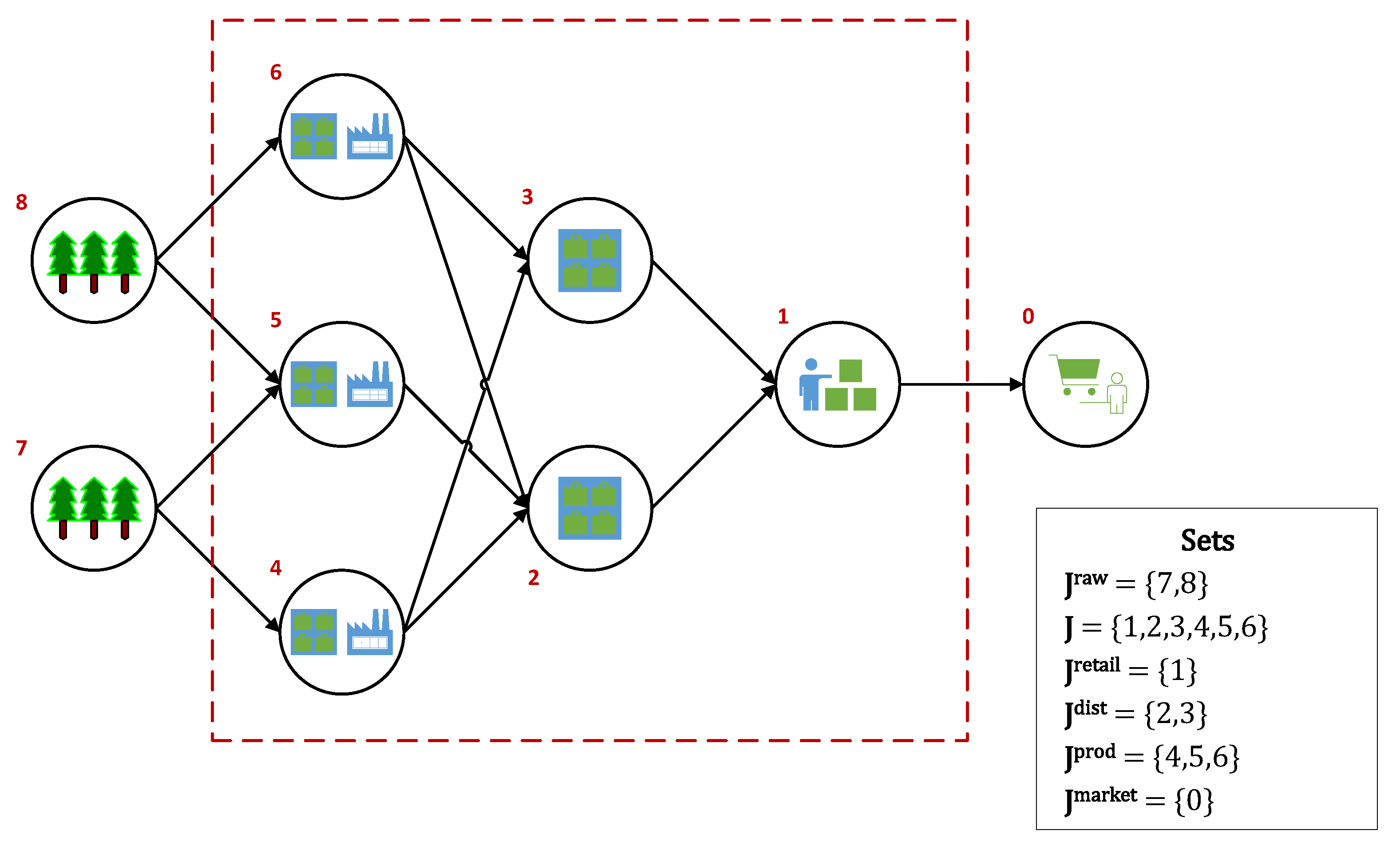
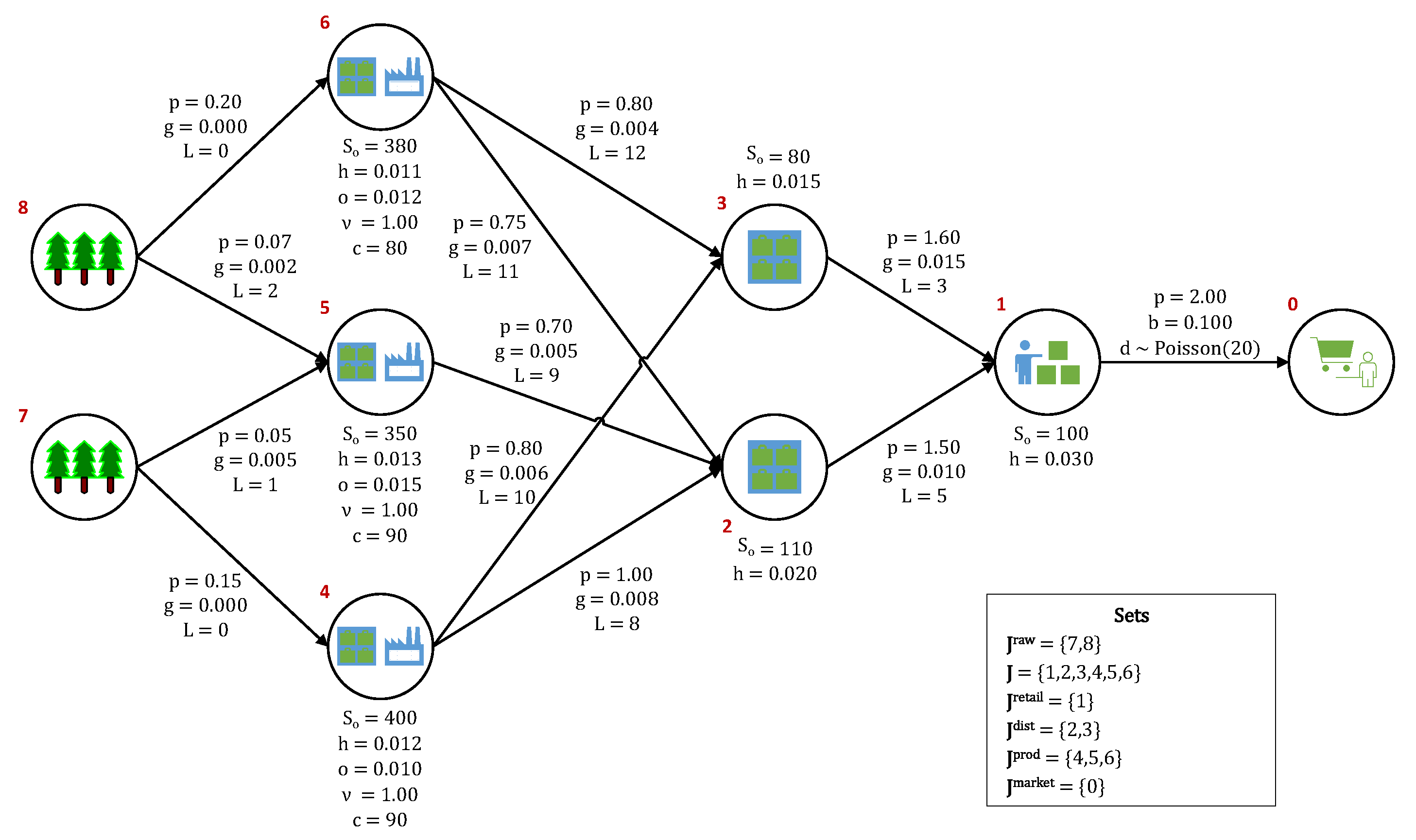
In this work, we focus on the multi-echelon, multi-period, single-product, and single-market inventory management problem (IMP) in a make-to-order supply network with uncertain stationary demand. The base case supply network has a tree topology with four echelons, as shown in Figure 1. The different sets that are used for the nodes in the base case network are designated in the figure’s legend (raw material, $J^{raw}$; main, J; retail, $J^{retail}$; distributor, $J^{dist}$; producer, $J^{prod}$; and, market nodes, $J^{market}$).

2.2. Sequence of Events

The sequence of events in each period of the IMP simulation environment occurs, as follows,

• Main network nodes (retailer, distributors, and producers) place replenishment orders to their respective suppliers. Replenishment orders are filled according to available production capacity and available feedstock inventory at the respective suppliers. The supply network is assumed to be centralized, such that replenishment orders never exceed what can be provided by the suppliers to each node.
• The main network nodes receive incoming feedstock inventory replenishment shipments that have made it down the product pipeline (after the associated lead times have transpired). The lead times between stages include both production times and transportation times.
• Single-product customer demand occurs at the retail node and it is filled according to the available inventory at that stage.
• One of the following occurs at the retailer node,

  (a)

  Unfulfilled sales are backlogged at a penalty. Backlogged sales take priority in the following period.

  (b)

  Unfulfilled sales are lost and a goodwill loss penalty is levied.

• Surplus inventory is held at each node at a holding cost. Inventory holding capacity limits are not included in the present formulation, but they can be easily added to the model, if needed. The IMP that is presented here is capacitated in the sense that manufacturing at production nodes is limited by both the production capacity and the availability of feedstock inventory at each node. Because the supply network operates as a make-to-order system, only feedstock inventories are held at the nodes. All of the product inventory is immediately shipped to the downstream nodes upon request, becoming feedstock inventory to those nodes (or simply inventory if the downstream node is a distributor/retailer). A holding (e.g., transportation) cost is also placed on any pipeline inventory (in-transit inventory).
• Any inventory remaining at the end of the last period (period 30 in the base case) is lost, which means that it has no salvage value.

2.3. Key Variables

Table 1. Main variables in the inventory management problem (IMP) Model.

Variable	Description
$a_{t,j,k}$	The reorder quantity requested to supplier node j by node k at the beginning of period t   (the amount of material sent from node j to node k)
$S_{t,j,k}^d$	The amount retailer j sells to market k in period $t-1$. Note: Retail sales are indexed at the   next period since these occur after demand in the current period is realized.
$S_{t,j}^o$	The on-hand inventory at node j just prior to when the demand is realized in period t.
$S_{t,j,k}^p$	The in-transit (pipeline) inventory between node j and node k just prior to when the demand   is realized in period t.
$u_{t,j,k}$	The unfulfilled demand at retailer j associated with market k in period $t-1$. Note: indexing is   also shifted since any unfulfilled demand occurs after the uncertain demand is realized.
$R_{t,j}$	The profit (reward) in node j for period t.

describes the main variables used in the IMP model. All of the key variables are continuous and non-negative.

2.4. Objective Function

The objective of the IMP optimization is to maximize the time-averaged expected profit of the supply network (R, Equation (1)). The uncertain parameter vector that is associated with the demand in period t is given by ${\xi }_{\mathit{t}}$. A specific realization of the uncertain parameter is denoted with ${\xi }_t$. The sequence of uncertain parameters from period t through $t^{\prime }$ is represented with ${\xi }_{[\mathit{t},{\mathit{t}}^{\prime }]}$, with ${\xi }_{[t,t]}$ being a specific realization of that sequence (note: ${\xi }_{[1,1]}$ refers to stage 1, which is deterministic). The present formulation assumes a single retailer–market link with a single demand in each period. The profit in each period is the sum of the profits in the main network nodes ($R_1={\sum }_{j\in J}{R}_{1,j}$ and $R_t={\sum }_{j\in J}{R}_{t,j}\left({\xi }_t\right)\forall t\in T$). The main network nodes include the production/manufacturing, distribution, and retail nodes.

$$maxR=\frac{1}{\left|T\right|}·\left(R_1+{\mathbb{E}}_{{\xi }_{[\mathbf{2},|\mathit{T}\left|\right]}|{\xi }_{[1,1]}}[max{R}_2\left({\xi }_2\right)+\dots +{\mathbb{E}}_{{\xi }_{\left[\right|\mathit{T}|,|\mathit{T}\left|\right]}|{\xi }_{[1,|T|-1]}}[max{R}_{\left|T\right|}\left({\xi }_{\left|T\right|}\right)]]\right)$$

(1)

2.5. IMP Model

The dynamics of the IMP under demand uncertainty are modeled as a Linear Programming (LP) problem using the linear algebraic constraints that are given below.

2.5.1. Network Profit

The profit in period t at node j ($R_{t,j}$, Equations (2a) and (2b)) is obtained by subtracting procurement costs ($P{C}_{t,j}$, Equations (4a) and (4b)), operating costs ($O{C}_{t,j}$, Equations (5a) and (5b)), unfulfilled demand penalties ($U{P}_{t,j}$, Equation (6)), and inventory holding costs ($H{C}_{t,j}$, Equations (7a) and (7b)) from the sales revenue ($S{R}_{t,j}$, and Equations (3a) and (3c)). The operating costs refer to production costs and, hence, do not apply to distribution nodes, as no manufacturing occurs at these nodes. There is also no unfulfilled demand at non-retail nodes, as all inter-network requests must be feasible.

In the equations shown below, the parameters $p_{j,k}$, $b_{j,k}$, and $g_{k,j}$ refer to the material unit price, the unfulfilled unit demand penalty, and the unit material pipeline holding cost (transportation cost) for the link going from node j to node k, respectively. $o_j$, ${\nu }_j$, and $h_j$ refer to the unit operating cost, production yield (0 to 1 range), and on-hand inventory holding cost at node j, respectively. The sets $J_j^{in}$ and $J_j^{out}$ are the sets of predecessors and successors to node j, respectively.

$$R_{1,j}=S{R}_{1,j}-P{C}_{1,j}-O{C}_{1,j}-U{P}_{1,j}-H{C}_{1,j}\forall j\in J$$

(2a)

$$R_{t,j}\left({\xi }_t\right)=S{R}_{t,j}\left({\xi }_t\right)-P{C}_{t,j}\left({\xi }_t\right)-O{C}_{t,j}\left({\xi }_t\right)-U{P}_{t,j}\left({\xi }_t\right)-H{C}_{t,j}\left({\xi }_t\right)\forall t\in \{2,\dots ,|T\left|\right\},j\in J$$

(2b)

$$S{R}_{1,j}=\sum _{k\in J_i^{out}}{p}_{j,k}·a_{1,j,k}\forall j\in J^{prod}\cup J^{dist}$$

(3a)

$$S{R}_{t,j}\left({\xi }_t\right)=\sum _{k\in J_i^{out}}{p}_{j,k}·a_{t,j,k}\left({\xi }_t\right)\forall t\in \{2,\dots ,|T\left|\right\},j\in J^{prod}\cup J^{dist}$$

(3b)

$$S{R}_{t,j}\left({\xi }_t\right)=\sum _{k\in J_i^{out}}{p}_{j,k}·S_{t,j,k}^d\left({\xi }_t\right)\forall t\in \{2,\dots ,|T\left|\right\},j\in J^{retail}$$

(3c)

$$P{C}_{1,j}=\sum _{k\in J_i^{in}}{p}_{k,j}·a_{1,k,j}\forall j\in J$$

(4a)

$$P{C}_{t,j}\left({\xi }_t\right)=\sum _{k\in J_i^{in}}{p}_{k,j}·a_{t,k,j}\left({\xi }_t\right)\forall t\in \{2,\dots ,|T\left|\right\},j\in J$$

(4b)

$$O{C}_{1,j}=\frac{o_j}{{\nu }_j}·\sum _{k\in J_j^{out}}{a}_{1,j,k}\forall j\in J^{prod}$$

(5a)

$$O{C}_{t,j}\left({\xi }_t\right)=\frac{o_j}{{\nu }_j}·\sum _{k\in J_i^{out}}{a}_{t,j,k}\left({\xi }_t\right)\forall t\in \{2,\dots ,|T\left|\right\},j\in J^{prod}$$

(5b)

$$U{P}_{t,j}\left({\xi }_t\right)=\sum _{k\in J_j^{out}}{b}_{j,k}·u_{t,j,k}\left({\xi }_t\right)\forall t\in \{2,\dots ,|T\left|\right\},j\in J^{retail}$$

(6)

$$H{C}_{1,j}=h_j·S_{1,j}^o+\sum _{k\in J_j^{in}}{g}_{k,j}·S_{1,k,j}^p\forall j\in J$$

(7a)

$$H{C}_{t,j}\left({\xi }_t\right)=h_j·S_{t,j}^o\left({\xi }_t\right)+\sum _{k\in J_j^{in}}{g}_{k,j}·S_{t,k,j}^p\left({\xi }_t\right)\forall t\in \{2,\dots ,|T\left|\right\},j\in J$$

(7b)

2.5.2. Inventory Balances

The on-hand inventory at each node is updated while using material balances that account for incoming and outgoing material, as shown in Equations (8a)–(9c). The inventory levels at each node are updated by adding any incoming inventory and subtracting any outgoing inventory to the previously recorded inventory levels at the respective nodes. The parameter $S_{0,j}^o$ is the initial inventory at node j. The variable $a_{t,k,j}^{\prime }$ is the pipeline inventory that arrives at node j from node k in period t (Equation (10)). Outgoing inventory is the inventory that is transferred to downstream nodes, $a_{t,j,k}$, or sold to the market at the retailer node, $S_{t,j,k}^d$. At production nodes, the sales quantities are adjusted for production yields (${\nu }_j$). For distribution nodes, ${\nu }_j$ is set to 1.

$$S_{1,j}^o=S_{0,j}^o+\sum _{k\in J_j^{in}}{a}_{1,k,j}^{\prime }-\frac{1}{{\nu }_j}·\sum _{k\in J_j^{out}}{a}_{1,j,k}\forall j\in J^{prod}\cup J^{dist}$$

(8a)

$$S_{2,j}^o\left({\xi }_2\right)=S_{1,j}^o+\sum _{k\in J_j^{in}}{a}_{2,k,j}^{\prime }-\frac{1}{{\nu }_j}·\sum _{k\in J_j^{out}}{a}_{2,j,k}\left({\xi }_2\right)\forall j\in J^{prod}\cup J^{dist}$$

(8b)

$$S_{t,j}^o\left({\xi }_t\right)=S_{t-1,j}^o\left({\xi }_{t-1}\right)+{\sum }_{k\in J_j^{in}}{a}_{t,k,j}^{\prime }-\frac{1}{{\nu }_j}·{\sum }_{k\in J_j^{out}}{a}_{t,j,k}\left({\xi }_t\right)t\in \{3,\dots ,|T\left|\right\}\forall j\in J^{prod}\cup J^{dist}$$

(8c)

$$S_{1,j}^o=S_{0,j}^o+\sum _{k\in J_j^{in}}{a}_{1,k,j}^{\prime }\forall j\in J^{retail}$$

(9a)

$$S_{2,j}^o\left({\xi }_2\right)=S_{1,j}^o+\sum _{k\in J_j^{in}}{a}_{2,k,j}^{\prime }-\sum _{k\in J_j^{out}}{S}_{2,j,k}^d\left({\xi }_2\right)\forall j\in J^{retail}$$

(9b)

$$S_{t,j}^o\left({\xi }_t\right)=S_{t-1,j}^o\left({\xi }_{t-1}\right)+\sum _{k\in J_j^{in}}{a}_{t,k,j}^{\prime }-\sum _{k\in J_j^{out}}{S}_{t,j,k}^d\left({\xi }_t\right)\forall t\in \{3,\dots ,|T\left|\right\},j\in J^{retail}$$

(9c)

$$a_{t,k,j}^{\prime }=\left\{\begin{array}{cc}0,\hfill & \mathrm{if}t-L_{k,j}<1\hfill \\ a_{1,k,j},\hfill & \mathrm{if}t-L_{k,j}=1\hfill \\ a_{t-L_{k,j},k,j}\left({\xi }_{t-L_{k,j}}\right),\hfill & \mathrm{if}t-L_{k,j}>1\hfill \end{array}\right.\forall t\in T,j\in J^{retail},k\in J_j^{in}$$

(10)

Equations (11a)–(11c) provide the pipeline inventory balances at each arc. Once again, inventories are updated by deducting delivered inventory downstream and adding new inventory requests to the previously recorded pipeline inventory levels. It is assumed that, at $t=0$, there is no inventory in the pipeline.

$$S_{1,k,j}^p=-a_{1,k,j}^{\prime }+a_{1,k,j}\forall j\in J,k\in J_j^{in}$$

(11a)

$$S_{2,k,j}^p\left({\xi }_2\right)=S_{1,k,j}^p-a_{2,k,j}^{\prime }+a_{2,k,j}\left({\xi }_2\right)\forall j\in J,k\in J_j^{in}$$

(11b)

$$S_{t,k,j}^p\left({\xi }_t\right)=S_{t-1,k,j}^p\left({\xi }_{t-1}\right)-a_{t,k,j}^{\prime }+a_{t,k,j}\left({\xi }_t\right)\forall t\in \{3,\dots ,|T\left|\right\},j\in J,k\in J_j^{in}$$

(11c)

2.5.3. Inventory Requests

Upper bounds on the replenishment orders are set, depending on the type of node. For the production nodes, downstream replenishment requests are limited by the production capacity, $c_j$, as given in Equations (12a) and (12b). The requests are also limited by the available feedstock inventory at the production nodes that is transformed into products with a yield of ${\nu }_j$, as stated in Equations (13a) and (13b). Because distribution-only nodes do not have manufacturing areas, the upper bounds on any downstream replenishment requests are set by the available inventory at the distribution nodes, which is equivalent to setting ${\nu }_j$ to 1 in Equations (13a) and (13b). These sets of constraints ensure that the reorder quantities are always feasible, which means that the quantities requested are quantities that can be sold and shipped in the current period.

$$\sum _{k\in J_j^{out}}{a}_{1,j,k}\le c_j\forall j\in J^{prod}$$

(12a)

$$\sum _{k\in J_j^{out}}{a}_{t,j,k}\left({\xi }_t\right)\le c_j\forall t\in \{2,\dots ,|T\left|\right\},j\in J^{prod}$$

(12b)

$$\sum _{k\in J_j^{out}}{a}_{1,j,k}\le S_{1,j}^o·{\nu }_j\forall j\in J^{prod}\cup J^{dist}$$

(13a)

$$\sum _{k\in J_j^{out}}{a}_{t,j,k}\left({\xi }_t\right)\le S_{t,j}^o\left({\xi }_t\right)·{\nu }_j\forall t\in \{2,\dots ,|T\left|\right\},j\in J^{prod}\cup J^{dist}$$

(13b)

2.5.4. Market Sales

The retailer node sells up to its available on-hand inventory in each period when the demand is realized, as given in Equations (14a) and (14b). This includes the start-of-period inventory plus any reorder quantities that arrive at the beginning of the period (before the markets open). Sales at the retailer nodes do not exceed the market demand, $d_{t,j,k}\left({\xi }_t\right)$, as shown in Equation (15a). If backlogging is allowed, then any previous backlogged orders are added to the market demand, as shown in Equation (15b). If unfulfilled orders are counted as lost sales, then u is removed from Equation (15b).

$$\sum _{k\in J_j^{out}}{S}_{2,j,k}^d\left({\xi }_2\right)\le S_{1,j}^o\forall j\in J^{retail}$$

(14a)

$$\sum _{k\in J_j^{out}}{S}_{t,j,k}^d\left({\xi }_t\right)\le S_{t-1,j}^o\left({\xi }_{t-1}\right)\forall t\in \{3,\dots ,|T\left|\right\},j\in J^{retail}$$

(14b)

$$S_{2,j,k}^d\left({\xi }_2\right)\le d_{2,j,k}\left({\xi }_2\right)\forall j\in J^{retail},k\in J_j^{out}$$

(15a)

$$S_{t,j,k}^d\left({\xi }_t\right)\le d_{t,j,k}\left({\xi }_t\right)+u_{t-1,j,k}\left({\xi }_{t-1}\right)\forall t\in \{3,\dots ,|T\left|\right\},j\in J^{retail},k\in J_j^{out}$$

(15b)

Unfulfilled demand at the retailer is the difference between the market demand and the actual retail sale in the current period (Equations (16a) and (16b). If the network operates under the lost sales mode, then the u term in the right-hand side of Equation (16b) is removed.

$$u_{2,j,k}\left({\xi }_2\right)=d_{2,j,k}\left({\xi }_2\right)-S_{2,j,k}^d\left({\xi }_2\right)\forall j\in J^{retail},k\in J_j^{market}$$

(16a)

$$u_{t,j,k}\left({\xi }_t\right)=d_{t,j,k}\left({\xi }_t\right)+u_{t-1,j,k}\left({\xi }_{t-1}\right)-S_{t,j,k}^d\left({\xi }_t\right)\forall t\in \{3,\dots ,|T\left|\right\},j\in J^{retail},k\in J_j^{market}$$

(16b)

2.5.5. Variable Domains

$$R_{1,j}\in {\mathbb{R}}^1\forall j\in J$$

(17a)

$$R_{t,j}\left({\xi }_t\right)\in \mathbb{R}\forall t\in \{2,\dots ,|T\left|\right\},j\in J$$

(17b)

$$S_{1,j}^o\ge 0\forall j\in J$$

(18a)

$$S_{t,j}^o\left({\xi }_t\right)\ge 0\forall t\in \{2,\dots ,|T\left|\right\},j\in J$$

(18b)

$$a_{1,k,j},S_{1,k,j}^p\ge 0\forall j\in J,k\in J_j^{in}$$

(19a)

$$a_{t,k,j}\left({\xi }_t\right),S_{t,k,j}^p\left({\xi }_t\right)\ge 0\forall t\in \{2,\dots ,|T\left|\right\},j\in J,k\in J_j^{in}$$

(19b)

$$S_{t,j,k}^d\left({\xi }_t\right),u_{t,j,k}\left({\xi }_t\right)\ge 0\forall t\in \{2,\dots ,|T\left|\right\},j\in J^{retail},k\in J_j^{out}$$

(20)

2.6. Scenario Tree for Multistage Stochastic Programming

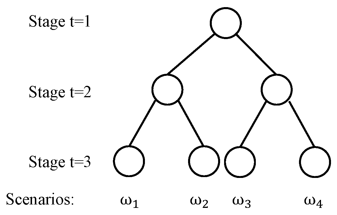
Equations (1)–(20) describe a multistage stochastic inventory management problem. In principle, continuous or discrete probability distributions can be used to model the uncertain demands in the stochastic process $({\xi }_1,{\xi }_2,\cdots ,{\xi }_t,\cdots ,{\xi }_{\left|T\right|})$. However, in most applications, a scenario-based approach is assumed for ease of computation, i.e., there are a finite number of realizations of the uncertain parameter. For illustration purposes, Figure 2 shows a scenario tree that corresponds to a three-stage stochastic programming problem. At stage one, the decision-maker does not know the realizations of the uncertain parameters in the future time periods. At stage two, there are two different realizations of the uncertain parameters. The decision-maker can take different actions, depending on the realization of the uncertainty at stage two. For each realization at stage two, there are two different realizations at stage three. Therefore, the scenario tree that is presented in Figure 2 has four scenarios in total.

It is easy to observe that the number of scenarios grows exponentially with respect to the number of stages. For example, in the IMP, if we consider three realizations of the demand per stage, the total number of scenarios will be $3^{29}$ for a 30 period problem. Moreover, a Poisson distribution is assumed for the distribution of the demand. In principle, there is an infinite number of realizations per stage. We introduce an approximation of the multistage stochastic programming problem in the next subsection in order to reduce the computational complexity.

2.7. Approximation for the Multistage Scenario Tree

In order to make the multistage stochastic IMP tractable, we make the following two simplifications.

First, the Poisson($\lambda$) distribution (as shown in Equation (21)) is approximated by a discrete distribution with three realizations.

$$p(x=k)=\frac{{\lambda }^k{e}^{-\lambda }}{k!}$$

(21)

Note that the mean and variance of Poisson ($\lambda$) are both $\lambda$. The values of the three realizations are chosen to be $\lambda -\sqrt{\lambda }$, $\lambda$, $\lambda +\sqrt{\lambda }$. The probabilities of the three realizations are chosen, such that the Wasserstein-1 distance to the original Poisson($\lambda$) is minimized. In other words, for all $k=1,2,\cdots ,\infty$, the probability of $x=k$ in Poisson ($\lambda$) is assigned to the realization of the new distribution that is closest to k. The probabilities for this new distribution are given in Equations (22a)–(22c).

$$p(x=\lambda -\sqrt{\lambda })=\sum _{k=1}^{\lambda -\frac{\sqrt{\lambda }}{2}}\frac{{\lambda }^k{e}^{-\lambda }}{k!}$$

(22a)

$$p(x=\lambda )=\sum _{k=\lambda -\frac{\sqrt{\lambda }}{2}+1}^{\lambda +\frac{\sqrt{\lambda }}{2}-1}\frac{{\lambda }^k{e}^{-\lambda }}{k!}$$

(22b)

$$p(x=\lambda +\sqrt{\lambda })=\sum _{k=\lambda +\frac{\sqrt{\lambda }}{2}}^{+\infty }\frac{{\lambda }^k{e}^{-\lambda }}{k!}$$

(22c)

This scenario generation approach, where the values of the realizations are fixed and the probabilities of each realization are chosen to minimize the Wasserstein-1 distance between the probability distribution of the scenario tree from the “true distribution”, has been reported in [23].

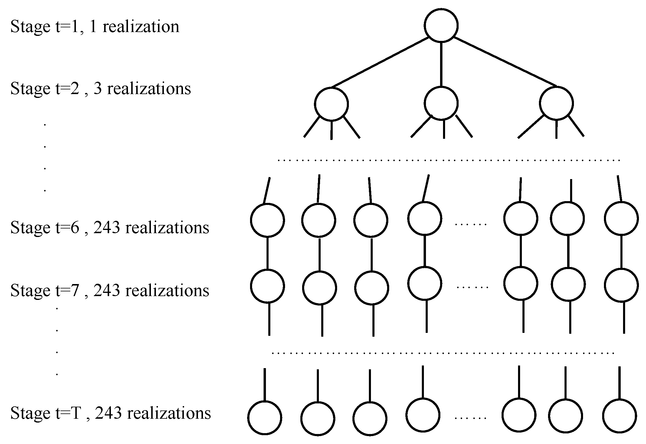
Second, even with three realizations per stage, the number of scenarios for $T=30$ becomes $3^{29}$. Because the decisions in the later periods have a smaller impact on the decisions here-and-now, we only consider three realizations per stage until stage 6. After stage 6, the demands are assumed to be deterministic and they take the mean value $\lambda$.

With these two simplifications, Figure 3 shows the scenario tree for the approximate multistage stochastic IMP. The size of the scenario tree grows exponentially until stage 6 and it only grows linearly after stage 6. In total, $3^5=243$ scenarios are considered. With slight abuse of notation, we still denote the problem that is shown in Figure 3 as MSSP.

2.8. Perfect Information and Deterministic Model

We benchmark the MSSP model with a perfection information model and a deterministic model. In the perfect information model, it is assumed that the demand realizations from $t=1$ to $t=T$ are known beforehand. Equation (1) reduces to Equation (23) in a perfect information model, where we assume that we know the realization of $({\xi }_2,\cdots ,{\xi }_t,\cdots ,{\xi }_{\left|T\right|})$ and optimize over this given realization.

$$maxR\left(\xi \right)=max\frac{1}{\left|T\right|}·\left(R_1+\sum _{t\in \{2,...,|T\left|\right\}}{R}_t\left({\xi }_t\right)\right)$$

(23)

In the deterministic model (DLP), we optimize over the expected value of ${\xi }_t$, which is denoted as $\overline{{\xi }_t}$. This means that the demand is assumed to be $\lambda$ (the mean of the Poisson distribution) for all periods.

2.9. Reinforcement Learning Model

Reinforcement learning (RL) is a machine learning method whereby an agent learns to maximize a reward via interactions with an environment. The feedback the agent receives from the reward allows it to learn a policy, which is a function that directs the agent at each step throughout the environment. Because of the data-intensive and interactive nature of RL, agents are typically trained by interacting with Monte Carlo simulations to make decisions at each time step.

To this end, we formulate the IMP as a Markov Decision Process (MDP)—a stochastic, sequential decision making problem. At each time period t, the agent observes the current state of the system ($S_t$), and then selects an action ($a_t$) that is passed to the system. The simulation then advances to the next state ($S_{t+1}$) based on the realization of the random variables and the selected action, and it returns the associated reward ($R_t$), which is simply the profit function that is given in Equation (2a) summed over all nodes j ($R_t={\sum }_{j\in J}{R}_{t,j}$).

The state consists of a vector with entries for the current demand at the retail node, the inventory levels at each node in the network, and the inventory in the pipeline along every edge in the network. In terms of the model notation from the previous subsection, $S_t=\{d_{t,j,k},S_{t,j}^o,S_{t,k^{\prime },j}^p|j\in J,k\in J_j^{out},k^{\prime }\in J_j^{in}\}$. The action at each period is a vector with all of the reorder quantities in the network ($a_t=\left\{a_{t,k,j}\right|j\in J,k\in J_j^{in}\}$).

In this work, we rely on the Proximal Policy Optimization (PPO), as described in Schulman et al. [24]. This has become a popular algorithm in the RL community, because it frequently exhibits stable learning characteristics. PPO is an actor-critic method that uses two neural networks that interact with one another. The actor is parameterized by ${\theta }_{\pi }$ and it learns the policy, while the critic is parameterized by ${\theta }_v$ and it learns the value function. The policy the actor learns is probabalistic in nature and yields a probability distribution over actions during each forward pass. For our IMP, the action space consists of re-order values for each node in the network. These are discrete values that range from 0 to the maximum order quantity at each individual node. If the actor chooses an action that is greater than the quantity that can be supplied – for example, if the maximum re-order quantity is 100, but only 90 units are available – then the minimum of these two values will be supplied.

The critic learns the value function, which allows it to estimate the sum of the discounted, future rewards available at each state. The difference between the actual rewards and the estimated rewards supplied by the critic is known as the temporal difference error (TD-error, or ${\delta }_T$). This difference is summed and discounted in order to provide the advantage estimation of the state, ${\widehat{A}}_k$, as given in Equation (24),

$${\widehat{A}}_k=\sum _{T=1}^t{\gamma }^{t-T+1}{\delta }_T$$

(24)

where $\gamma$ is the discount factor used to prioritize current rewards over future rewards. This value is then used in the loss function, $\mathcal{L}\left(\theta \right)$, whereby the paramaters of the networks are updated while using stochastic gradient descent to minimize the loss function. PPO has shown to be effective in numerous domains, exhibiting stable learning features, as discussed in Schulman et al. [24]. PPO achieves this by penalizing large policy updates by optimizing a conservative loss function given by Equation (25), where $r_k\left(\theta \right)$ is the probability ratio between the new policy ${\pi }_k\left(\theta \right)$ and the previous policy, ${\pi }_{k-1}\left(\theta \right)$. Here, we use k to denote each policy iteration, since the parameters have been initialized. The clip function reduces the incentive for moving $r_k\left(\theta \right)$ outside the interval $[1-ϵ,1+ϵ]$. The hyperparameter $ϵ$ limits the update of the policy, such that the probability of outputs does not change more than $\pm ϵ$ at each update. For more detail, see the work by Schulman et al. [24].

$$\mathcal{L}\left(\theta \right)=min\left(r_k\left(\theta \right){\widehat{A}}_k,\mathrm{clip}\left(r_k\left(\theta \right),1-ϵ,1+ϵ\right){\widehat{A}}_k\right)$$

(25)

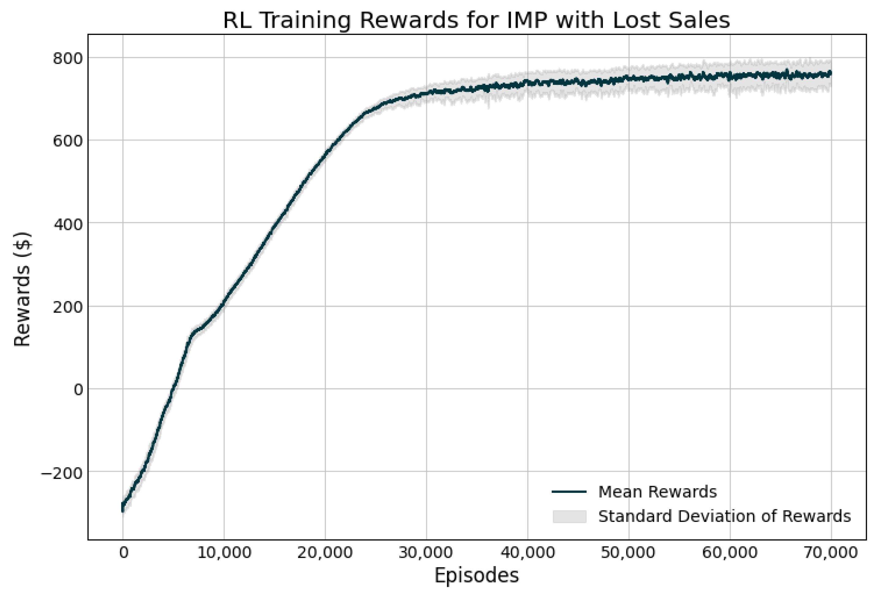
In the present work, we rely on the implementation of the PPO algorithm found in the Ray package [25]. A two-layer, 256-node feed-forward network is trained with over 70,000 episodes—simulated 30-day periods, whereby the agent learns to maximize the expected reward by interacting with the environment. Given that this is a model-free approach, the agent must learn through this trial-and-error approach. The initial policy consists of randomly initialized weights and biases, so the output actions are on par with random decisions. After each episode, the results are collected and the weights and biases are updated in order to minimize the loss function according to the PPO algorithm, as discussed in Section 2.9. As one would expect, this initial policy performs poorly, with the agent losing roughly $300 per episode. However, as shown in the training curve presented in Figure 4, the agent is able to improve on the policy with additional experience and learn a very effective policy to control the inventory across the network.

2.10. Case Study

A 30-period system is used for the case study in order to represent one month’s worth of inventory management in a supply network. A time step of one day is used, such that demand is received on a daily basis. Figure 5 depicts the network structure of the base case system used. Major parameters and their values are included in the figure. Parameters that are next to nodes are specific to the node (initial state or on-hand inventory, $S_0$; unit holding costs, h; unit operating costs, o; production yield $\nu$; and, production capacity, c), whereas those next to links are specific to that link (unit sales price, p; unfulfilled unit demand penalty, b; market demand distribution, d; unit pipeline holding costs, g; and, lead times, L). Node and link subscripts in the schematic are dropped for clarity. In order to compare the performance of the three modeling approaches (DLP, MSSP, and RL), 100 unique sample paths were generated. Each sample path consists of 30 demand realizations, one for each period in the simulation horizon, sampled from a Poisson distribution with a mean of 20.

The execution of the 100 simulations follows the sequence of events for each time period that is described in Section 2.2. At the beginning of each period and prior to Step 1 in the event sequence, each optimization model is called to obtain the reorder quantities for each node in that period. The models have no knowledge of the demand realizations that will occur in the current and future periods, but they can rely on the variables/states from previous periods. The reorder quantities for the current period obtained by the models are then passed as the actions in Step 1 of the sequence of events. Subsequently, the subsequent events for that period unfold, with the demand realization for that given period being taken from the respective sample path that is assigned to that simulation instance. The process is repeated for the next period, re-solving the models at the beginning of each time period, until the 30 periods are complete.

The three modeling approaches are benchmarked against a perfect information model (also referred to as the Oracle). 10-period windows are used for the rolling horizon (RH) modes in the DLP and MSSP models. However, towards the end of the simulation, the RH becomes a shrinking horizon (SH), since the window does not roll past period 30.

3. Results

The DLP and MSSP models were solved while using Gurobi (version 9.1). The DLP models are quite small, with the largest one being the DLP-SH solved at $t=1$ in the simulations (1231 constraints and 1291 variables). The DLP-RH with a 10-period window size has 411 constraints and 431 variables. The shrinking and rolling horizon DLP models both have CPU solve times that are below 0.3 s on average. The largest MSSP model solved is the MSSP-SH solved at $t=1$ (263,958 constraints and 299,941 variables), which has an average CPU solve time of 119 s. The MSSP-RH with a 10-period window size has 64,698 constraints and 71,521 variables. The average CPU time to solve the MSSP-RH model is 12 s.

Table 2. Total reward comparison for the various models used to solve the IMP. Performance Ratio is defined as the ratio of the final cumulative profit of the perfect information model to that of the model used. DLP = Deterministic linear program; MSSP = Multi-stage stochastic program; RL = Reinforcement Learning; RH = rolling horizon; SH = shrinking horizon; Oracle = perfect information LP.

	DLP-RH	DLP-SH	MSSP-RH	MSSP-SH	RL	Oracle
Backlog
Mean Profit	791.6	825.3	802.7	847.7	737.2	861.3
Standard Deviation	52.5	37.0	56.3	49.4	24.8	56.4
Performance Ratio	1.09	1.04	1.07	1.02	1.17	1.00
Lost Sales
Mean Profit	735.8	786.9	790.6	830.6	757.8	854.9
Standard Deviation	31.2	30.8	47.8	37.7	33.1	49.9
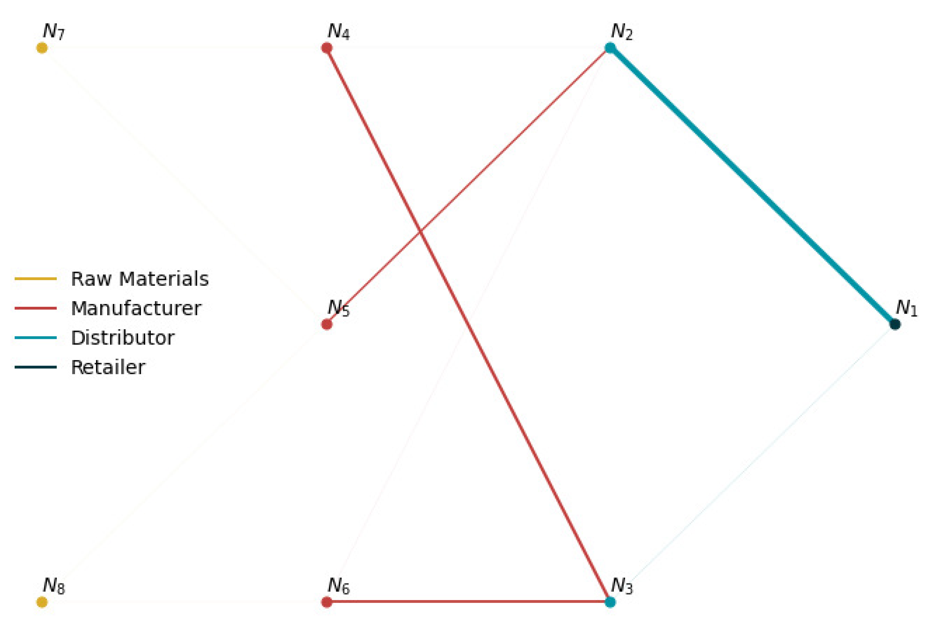
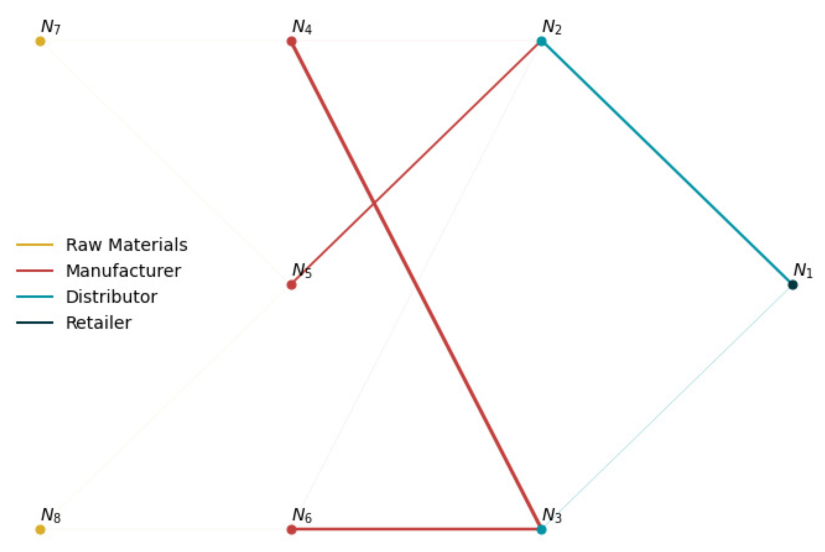
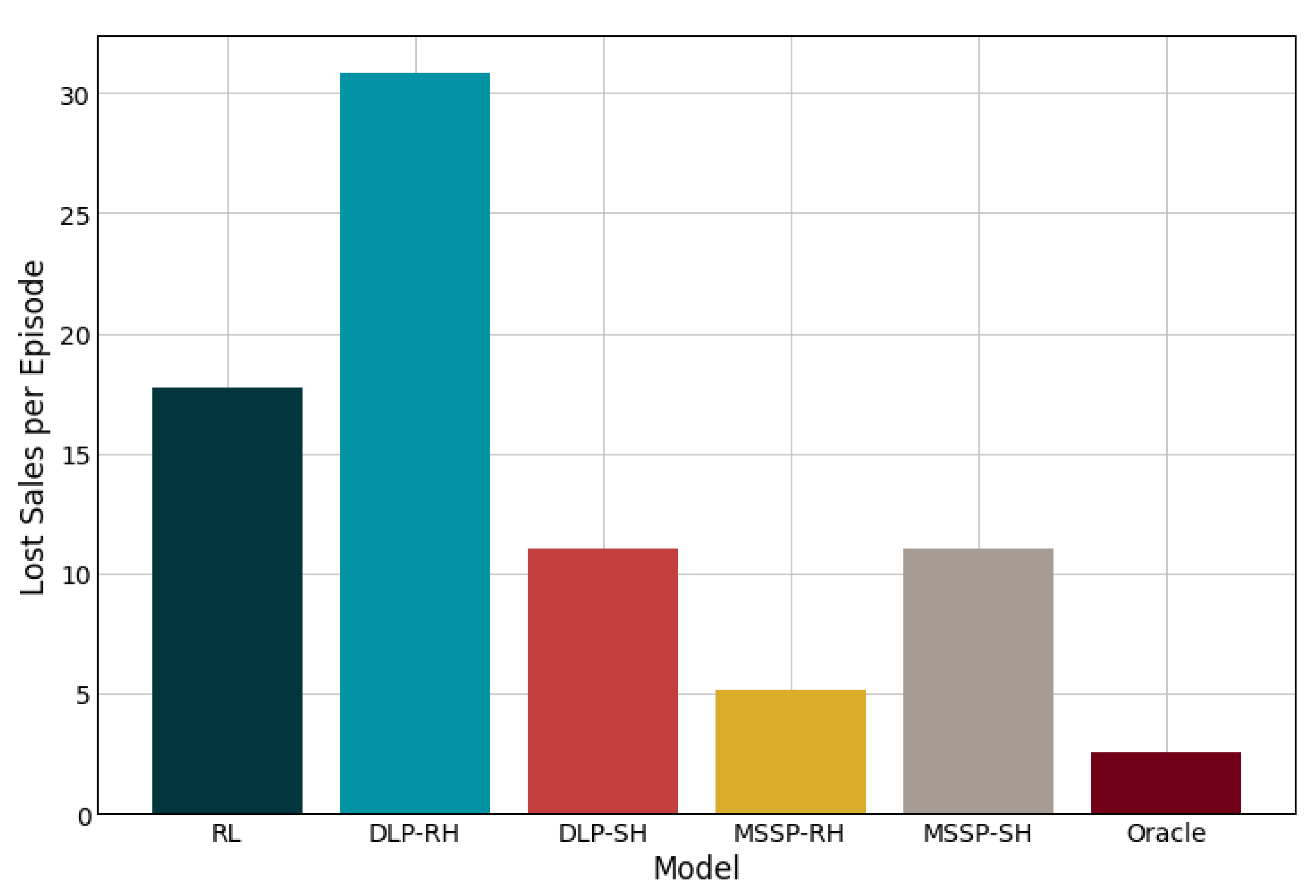
Performance Ratio	1.16	1.09	1.08	1.03	1.13	1.00

summarizes the performance results from each solution method. Figure 6 shows the total inventory profiles at each node for the lost sales case. The total inventory includes both on-hand inventory and pipeline inventory incoming from a node’s suppliers. Similar results (not shown) were observed for the backlogging case. Figure 7 and Figure 8 show sample network flow plots for the RL and MSSP-RH models, respectively. The cumulative network flow plots for both DLP instances and MSSP-SH are not shown as they are similar to that of MSSP-RH. The edge thickness is proportional to the average total amount of material requested through that link. These network flows indicate the suppliers that are prioritized by the different model policies. Figure 9 shows the average unfulfilled market demand at the retailer node (lost sales), which gives an indication of the service levels of the supply network. A similar result is obtained for the backlogging case.

4. Discussion

The results shown in Table 2 indicate that the rolling horizon DLP model outperforms the RL model when backlog is included, but it is outperformed by the latter when unfulfilled demands become lost sales. When backlogging is allowed, unfulfilled demand can be satisfied at a later period with a penalty, which reduces the need for high service levels. However, the service levels become more important in the lost sales case, where, not only is a goodwill penalty assessed, but potential profit from the sales is lost. Because the RL does a better job at maintaining on-hand inventories it displays the higher service levels shown in Figure 9 and superior performance in the lost sales case. It should be noted that the differences between the two approaches are rather small (7% and 3%, respectively), and within 15% of the perfect information model.

As expected, the shrinking horizon DLP exhibits superior performance relative to its rolling horizon counterpart, because it looks further ahead in time during the optimization. In the rolling horizon approach, the short-sighted model tends to drop inventory levels at the top tier suppliers (nodes 4–6) sooner in an attempt to reduce the inventory holding costs towards the end of the optimization window. However, since the simulation horizon extends beyond the 10-period optimization window, that inventory ends up accumulating in the medium tier suppliers (nodes 2–3), driving up holding costs overall. From a service level standpoint, the shrinking horizon DLP maintains higher inventory levels at the retailer than its rolling horizon counterpart, allowing it to achieve higher service levels (see Figure 9). However, it is interesting to note that the opposite is observed in the MSSP model, which, despite having a higher profit, has lower service levels in the shrinking horizon case (higher unfulfilled demand). The greater profit is a result of the shrinking horizon reducing holding costs by 13% overall, which has a greater impact on profit than the unfulfilled demand penalties. Just at the retailer node, the holding cost to demand penalty ratio is 3:1, which incentivizes the model to sacrifice some demand satisfaction to reduce the holding costs. Overall, the MSSP model yields superior performance in all cases, coming in within 8% and 3% of the best possible outcome (Oracle), on average, for the rolling horizon and shrinking horizon modes, respectively.

From an operational standpoint, the Oracle and shrinking horizon models prioritize inventory flow to the retailer via nodes 5 and 2, which have a lower holding cost than the alternatives as shown in the timing of inventory transfers in Figure 6 and the flow patterns in Figure 8. The transportation cost for this path is 0.015, with a lead time of 14 days, whereas the other paths have transportation costs in the range 0.017–0.021, with lead times in the 13–16 day range. Once inventory at node 5 is depleted, the other top level suppliers (nodes 4 and 6) begin to send inventory downstream. On the other hand, the rolling horizon models send inventory from all of the top level suppliers from the start due to the myopic effects of the reduced optimization window. In general terms, the inventory profiles that are shown in Figure 6 for the rolling horizon models are similar to their shrinking horizon counterparts, except that the inventory changes are shifted to earlier times. All of the mathematical programming models also take advantage of the fact that the pipeline inventory costs are lower than holding costs at the supplier nodes. Therefore, they trigger sending more inventory to node 3 from nodes 4 and 6 than is needed so as to reduce costs. This additional inventory ends up accumulating in node 3 for the most part, as it is cheaper to source the retailer from node 2 than node 3. Although the DLP and MSSP models exhibit similar inventory profiles, the superiority of the MSSP model arises from the fact that, unlike the DLP model, it accounts for uncertainty in the demand, which enables it to target superior service levels and reduce holding costs.

In contrast to the mathematical programming models, the RL model avoids drastic changes in the inventory positions, maintaining levels throughout the simulation. This is supported not only by the inventory levels in Figure 6, but also by the flow pattern shown in Figure 7, which indicate that, contrary to the mathematical programming models, the RL model distributes requests more evenly amongst the suppliers of each node. This conservative approach explains why the profits obtained with the RL model are lower than those that were obtained by most of mathematical programming models. In practice, the policy from the RL model is preferred as it reduces shocks to the inventory levels. Furthermore, the RL policy manages the supply network with potentially greater resiliency to disruptions as a result of the balanced load distribution within the network. Unlike the other models that have virtually no flow between the raw material nodes to the top tier suppliers and rely solely on the initial inventory at these nodes, the RL model gradually replenishes inventories at the top tier nodes in order to avoid their depletion. This conservative behavior of the RL is observed as a result of the PPO algorithm used, which penalizes large policy changes.

A drawback from the current implementation of the supply network is that all of the models exhibit end-of-simulation effects, in which the inventory drops to zero or near zero at the end of the simulation to avoid excess holding costs. In a real application, this could be avoided by imposing penalties on the models in order to avoid depleting inventories near the end of the simulation, adding terminal inventory constraints (Lima et al. [26]), or running the models for longer simulation horizons, since most of the applications extend beyond 30 periods. The latter option would not be viable for the stochastic programming models as it would affect their tractability. Despite these limitations, the three approaches show promise in obtaining dynamic reorder policies that improve the supply network performance to within 3% to 15% of perfect information dynamic policies, which do not exist in practice.

5. Conclusions

The present work extends to the open-source package OR-Gym for general single-product, multi-period make-to-order supply networks with production and inventory holding sites throughout the network. The work introduces additional tools for solving inventory management problems within the OR-Gym framework (e.g. multi-stage stochastic programming and rolling horizon implementations for deterministic and stochastic models). The inventory management policies that are obtained via deterministic linear programming, stochastic linear programming, and reinforcement learning are compared and contrasted in the context of a four echelon supply network with uncertain stationary demand. The results show that the stochastic model yields superior results in terms of supply network profitability. However, the reinforcement learning model manages the network in a way that is potentially more resilient to network disruptions, showing promise in using AI for supply chain applications. Although deterministic linear models ignore the stochastic nature of the supply network, they rapidly solve in fractions of a second, while providing solutions that are comparable to the profitability of the reinforcement learning policies. Extensions to this work may include studying the effects of non-stationary demand on the models used and mitigating the end-of-simulation effects that have been discussed previously.

References

- Lee, H.L.; Padmanabhan, V.; Whang, S. Information distortion in a supply chain: The bullwhip effect. Manag. Sci. 1997, 43, 546–558. [Google Scholar] [CrossRef]
- Eruguz, A.S.; Sahin, E.; Jemai, Z.; Dallery, Y. A comprehensive survey of guaranteed-service models for multi-echelon inventory optimization. Int. J. Prod. Econ. 2016, 172, 110–125. [Google Scholar] [CrossRef]
- Simchi-Levi, D.; Zhao, Y. Performance Evaluation of Stochastic Multi-Echelon Inventory Systems: A Survey. Adv. Oper. Res. 2012, 2012, 126254. [Google Scholar] [CrossRef] [Green Version]
- Glasserman, P.; Tayur, S. Sensitivity analysis for base-stock levels in multiechelon production-inventory systems. Manag. Sci. 1995, 41, 263–281. [Google Scholar] [CrossRef]
- Chu, Y.; You, F.; Wassick, J.M.; Agarwal, A. Simulation-based optimization framework for multi-echelon inventory systems under uncertainty. Comput. Chem. Eng. 2015, 73, 1–16. [Google Scholar] [CrossRef]
- Dillon, M.; Oliveira, F.; Abbasi, B. A two-stage stochastic programming model for inventory management in the blood supply chain. Int. J. Prod. Econ. 2017, 187, 27–41. [Google Scholar] [CrossRef]
- Fattahi, M.; Mahootchi, M.; Moattar Husseini, S.M.; Keyvanshokooh, E.; Alborzi, F. Investigating replenishment policies for centralised and decentralised supply chains using stochastic programming approach. Int. J. Prod. Res. 2015, 53, 41–69. [Google Scholar] [CrossRef]
- Pauls-Worm, K.G.; Hendrix, E.M.; Haijema, R.; Van Der Vorst, J.G. An MILP approximation for ordering perishable products with non-stationary demand and service level constraints. Int. J. Prod. Econ. 2014, 157, 133–146. [Google Scholar] [CrossRef]
- Zahiri, B.; Torabi, S.A.; Mohammadi, M.; Aghabegloo, M. A multi-stage stochastic programming approach for blood supply chain planning. Comput. Ind. Eng. 2018, 122, 1–14. [Google Scholar] [CrossRef]
- Bertsimas, D.; Thiele, A. A robust optimization approach to inventory theory. Oper. Res. 2006, 54, 150–168. [Google Scholar] [CrossRef]
- Govindan, K.; Cheng, T.C. Advances in stochastic programming and robust optimization for supply chain planning. Comput. Oper. Res. 2018, 100, 262–269. [Google Scholar] [CrossRef]
- Roy, B.V.; Bertsekas, D.P.; North, L. A neuro-dynamic programming approach to admission control in ATM networks. In Proceedings of the IEEE International Conference on Acoustics, Speech, and Signal Processing, Munich, Germany, 21–24 April 1997. [Google Scholar]
- Kleywegt, A.J.; Non, V.S.; Savelsbergh, M.W. Dynamic Programming Approximations for a Stochastic Inventory Routing Problem. Transport. Sci. 2004, 38, 42–70. [Google Scholar] [CrossRef]
- Topaloglu, H.; Kunnumkal, S. Approximate dynamic programming methods for an inventory allocation problem under uncertainty. Naval Res. Logist. 2006, 53, 822–841. [Google Scholar] [CrossRef] [Green Version]
- Kunnumkal, S.; Topaloglu, H. Using stochastic approximation methods to compute optimal base-stock levels in inventory control problems. Oper. Res. 2008, 56, 646–664. [Google Scholar] [CrossRef] [Green Version]
- Cimen, M.; Kirkbride, C. Approximate dynamic programming algorithms for multidimensional inventory optimization problems. In Proceedings of the 7th IFAC Conference on Manufacturing, Modeling, Management, and Control, Saint Petersburg, Russia, 19–21 June 2013; Volume 46, pp. 2015–2020. [Google Scholar] [CrossRef]
- Sarimveis, H.; Patrinos, P.; Tarantilis, C.D.; Kiranoudis, C.T. Dynamic modeling and control of supply chain systems: A review. Comput. Oper. Res. 2008, 35, 3530–3561. [Google Scholar] [CrossRef]
- Mortazavi, A.; Arshadi Khamseh, A.; Azimi, P. Designing of an intelligent self-adaptive model for supply chain ordering management system. Eng. Appl. Artif. Intell. 2015, 37, 207–220. [Google Scholar] [CrossRef]
- Oroojlooyjadid, A.; Nazari, M.; Snyder, L.; Takáč, M. A Deep Q-Network for the Beer Game: A Reinforcement Learning algorithm to Solve Inventory Optimization Problems. arXiv 2017, arXiv:1708.05924. [Google Scholar]
- Kara, A.; Dogan, I. Reinforcement learning approaches for specifying ordering policies of perishable inventory systems. Expert Syst. Appl. 2018, 91, 150–158. [Google Scholar] [CrossRef]
- Sultana, N.N.; Meisheri, H.; Baniwal, V.; Nath, S.; Ravindran, B.; Khadilkar, H. Reinforcement Learning for Multi-Product Multi-Node Inventory Management in Supply Chains. arXiv 2020, arXiv:2006.04037. [Google Scholar]
- Hubbs, C.D.; Perez, H.D.; Sarwar, O.; Sahinidis, N.V.; Grossmann, I.E.; Wassick, J.M. OR-Gym: A Reinforcement Learning Library for Operations Research Problems. arXiv 2020, arXiv:2008.06319. [Google Scholar]
- Hochreiter, R.; Pflug, G.C. Financial scenario generation for stochastic multi-stage decision processes as facility location problems. Ann. Oper. Res. 2007, 152, 257–272. [Google Scholar] [CrossRef]
- Schulman, J.; Moritz, P.; Levine, S.; Jordan, M.I.; Abbeel, P. High-dimensional continuous control using generalized advantage estimation. arXiv 2016, arXiv:1506.02438. [Google Scholar]
- Moritz, P.; Nishihara, R.; Wang, S.; Tumanov, A.; Liaw, R.; Liang, E.; Elibol, M.; Yang, Z.; Paul, W.; Jordan, M.I.; et al. Ray: A Distributed Framework for Emerging AI Applications. In Proceedings of the 13th USENIX Symposium on Operating Systems Design and Implementation (OSDI 18), Carlsbad, CA, USA, 8–10 October 2018. [Google Scholar]
- Lima, R.M.; Grossmann, I.E.; Jiao, Y. Long-term scheduling of a single-unit multi-product continuous process to manufacture high performance glass. Comput. Chem. Eng. 2011, 35, 554–574. [Google Scholar] [CrossRef]
Figure 1.
Supply Chain Network Schematic.
Figure 2.
The scenario tree for a three-stage stochastic program with two realizations per stage.
Figure 3.
An approximation of the multistage stochastic program.
Figure 4.
Training curve for the reinforcement learning (RL) model.
Figure 5.
Supply Chain Network Schematic with Network Parameters used in the Case Study.
Figure 6.
Average total inventory at each main network node (lost sales mode). Shaded areas denote standard deviation of the mean value.
Figure 7.
Average network flow with the RL policy (lost sales mode). Total flow is proportional to the edge thickness.
Figure 8.
Average network flow with the MSSP-RH policy (lost sales mode). Total flow is proportional to the edge thickness.
Figure 9.
Average unfulfilled demands at the retailer node (lost sales mode).