
Material Generation Algorithm: A Novel Metaheuristic Algorithm for Optimization of Engineering Problems


1
Department of Civil Engineering, University of Tabriz, Tabriz 5166616471, Iran
2
Engineering Faculty, Near East University, North Cyprus, Mersin 10, Turkey
3
Faculty of Engineering & Information Technology, University of Technology Sydney, Ultimo, Sydney, NSW 2007, Australia
*
Author to whom correspondence should be addressed.
Processes 2021, 9(5), 859; https://0-doi-org.brum.beds.ac.uk/10.3390/pr9050859
Submission received: 30 March 2021
/
Revised: 3 May 2021
/
Accepted: 10 May 2021
/
Published: 13 May 2021
(This article belongs to the Special Issue Evolutionary Process for Engineering Optimization)
Abstract
:A new algorithm, Material Generation Algorithm (MGA), was developed and applied for the optimum design of engineering problems. Some advanced and basic aspects of material chemistry, specifically the configuration of chemical compounds and chemical reactions in producing new materials, are determined as inspirational concepts of the MGA. For numerical investigations purposes, 10 constrained optimization problems in different dimensions of 10, 30, 50, and 100, which have been benchmarked by the Competitions on Evolutionary Computation (CEC), are selected as test examples while 15 of the well-known engineering design problems are also determined to evaluate the overall performance of the proposed method. The best results of different classical and new metaheuristic optimization algorithms in dealing with the selected problems were taken from the recent literature for comparison with MGA. Additionally, the statistical values of the MGA algorithm, consisting of the mean, worst, and standard deviation, were calculated and compared to the results of other metaheuristic algorithms. Overall, this work demonstrates that the proposed MGA is able provide very competitive, and even outstanding, results and mostly outperforms other metaheuristics.
1. Introduction
Optimization techniques have been proposed for the optimum design of different problems of everyday life in order to increase the efficiency of systems and human resources. Most of the design problems in nature are complex, with multiple design variables and constraints that classical optimization algorithms, such as gradient-based algorithms, cannot handle. As a solution, numerous artificial intelligence experts have introduced new algorithms with better performance in different fields. Regarding the recent developments in technology, new optimization methods offering higher efficiency, greater accuracy, and increased speed rate are required to deal with difficult optimization problems.
Based on the mentioned concerns about the capabilities of optimization algorithms, a “metaheuristic” approach has been proposed by optimization experts [1] for solving different optimization problems. ‘Metaheuristic’ refers to specific solution techniques, where higher-level strategies are implemented into the main searching process of the optimization algorithms to provide a powerful searching method with specific capabilities, including the avoidance of entrapment in local optimal solutions. The history of developing different metaheuristic approaches as solutions in different optimization fields can be classified into five different time periods. A brief summary of these historical time periods is presented in Table 1.
With the evolution of numerous metaheuristic algorithms, four different types could be distinguished in terms of their main concepts and inspirations. The first category includes “evolutionary algorithms,” such as the Memetic Algorithm (MA) [3], Genetic Algorithm (GA) [4], Genetic Programming (GP) [5], Differential Evolution (DE) [6], Evolution Strategies (ES) [7], and the Biogeography-Based Optimizer (BBO) [8], that have been proposed based on the biological reproduction and evolution. The second category contains swarm intelligence-based optimization algorithms, which are based on the cooperative behavior of self-organized and decentralized artificial or natural systems. Some well-known methods of this category are Particle Swarm Optimization (PSO) [9], Ant Colony Optimization (ACO) [10], Artificial Bee Colony (ABC) [11], Cat Swarm Optimization (CSA) [12], Firefly Algorithm (FA) [13], and Krill Herd (KH) algorithm [14]. The third category consists of algorithms that are motivated by physical laws, such as Simulated Annealing (SA) [15], Harmony Search (HS) [16], Big-Bang Big-Crunch (BBBC) [17], Gravitational Search Algorithm (GSA) [18], Charged System Search (CSS) algorithm [19], Artificial Chemical Reaction Optimization Algorithm (ACROA) [20], Colliding Bodies Optimization (CBO) [21], Chaos Game Optimization (CGO) [22,23], and Atomic Orbital Search (AOS) [24] algorithm. Finally, metaheuristic approaches inspired by the lifestyle of animals or humans are classified in the fourth category, which includes Imperialistic Competitive Algorithm (ICA) [25], Cuckoo Search Algorithm (CSA) [26]. In addition to these metaheuristic algorithms, other difficult challenges have been solved by upgrading, developing, and hybridizing standard algorithms [27,28,29,30,31,32,33,34,35,36].
In this paper, a novel metaheuristic algorithm called the Material Generation Algorithm (MGA) is proposed as an alternative approach for solving optimization problems. The main concept of this novel algorithm is based on the principles of chemistry, regarding the production of new materials according to the configurations of chemical compounds and reactions. To evaluate the performance of MGA, we tested it on 15 well-known engineering design problems and 10 constrained mathematical problems in different dimensions (10, 30, 50, and 100), which have been benchmarked by the Competitions on Evolutionary Computation (CEC) and presented in detail by Wu et al. [37] at CEC 2017. The utilized references include the results of CEC 2017, Tvrdík and Poláková [38], Polakova [39], and Zamuda [40]. The Friedman Test [41] is also conducted as a well-known statistical test in order to have a fair judgment about the performance of the MGA.
In recent decades there has be a great challenge for the algorithm developers to develop new solution methods which could have better performance than the previous methods in dealing with complex real-world problems. Due to the massive emergence of novel metaheuristic algorithms in the past few decades, this aspect has been addressed by Sorensen [42] as a tsunami of methods which will have advantages and also disadvantages in the soft computing fields in the future. However, this issue can be justified by discovering other aspects of proposing novel algorithms which is based on the source of inspirational concept of a novel algorithm which should be reasonable enough to be justified alongside a well-developed mathematical model as two of the most important principles of metaheuristic algorithms. Regarding the fact that when a novel algorithm is proposed, it is evaluated by some of the benchmark test problems which has been solved by multiple methods in order to demonstrate its capability as an independent algorithm among the other methods while this kind of proposing a testing the algorithms is not the only aim of this area. The proposed novel algorithm can be of a great help in the situations that the other alternatives cannot reach to a reasonable response in dealing with a considered problem so there should be other alternatives in order to have a good chance to provide a well-designed plan for the industry and even human-related actions in the everyday life. A brief outline of this work is as follows:
Section 2 discusses the inspirational concept and mathematical model of the MGA optimization algorithm. In Section 3, the problem statements, including the selected mathematical and engineering optimization problems utilized to test the proposed MGA as a novel metaheuristic algorithm, are presented. In Section 4 and Section 5, the numerical results of the MGA algorithm and other alternative metaheuristic methods in dealing with the considered mathematical and engineering optimization problems are presented. In Section 6, the key findings of this research work are concluded, future research directions are suggested.
2. Material Generation Algorithm
In this section, the inspiration of MGA as a novel metaheuristic algorithm and the mathematical model of this algorithm are presented.
2.1. Inspiration
A material is a mixture of multiple substances comprised of the stuffs of the universe with volume and mass. The material generation process concerns the capability of different substances to merge with each other in order to generate new materials with higher functionality and improved energy levels. Elements are the basic building blocks of the materials, which cannot be broken into parts or even changed into other elements. Materials are engineered on an atomic, nano-, micro-, or macro-scale in order to control the specific properties and improve the performance of a material. Uniquely-generated materials are classified based on their general properties and specific characteristics and according to physical and chemical changes that influence a material’s behavior.
Material chemistry is one of the most important disciplines in the material research field. Material engineers study the configuration of materials in order to improve the specific characteristics of materials, developing new ones that are more sustainable and also superior to the previous ones. Chemical changes in materials are achieved by reacting and combining various chemicals. In general, the chemical properties are altered by the transferring or sharing of electrons between atoms of different materials, specifically, chemical bonds formed between materials result in such modifications. In this work, three main concepts of material chemistry (compounds, reactions, and stability) were considered to formulate a metaheuristic optimization algorithm.
2.1.1. Chemical Compound
Most chemical elements in the universe are created through combinations with other elements. With that being, a few chemical elements exist freely in nature. Compounds are formed by combining multiple chemicals via chemical bonds, or the transferring or sharing of electrons, which result in one of the following:
- -
- Ionic compounds are created when electrons are transferred from the atoms of one element to those of another.
- -
- Covalent compounds form when electrons are shared between atoms of different elements.
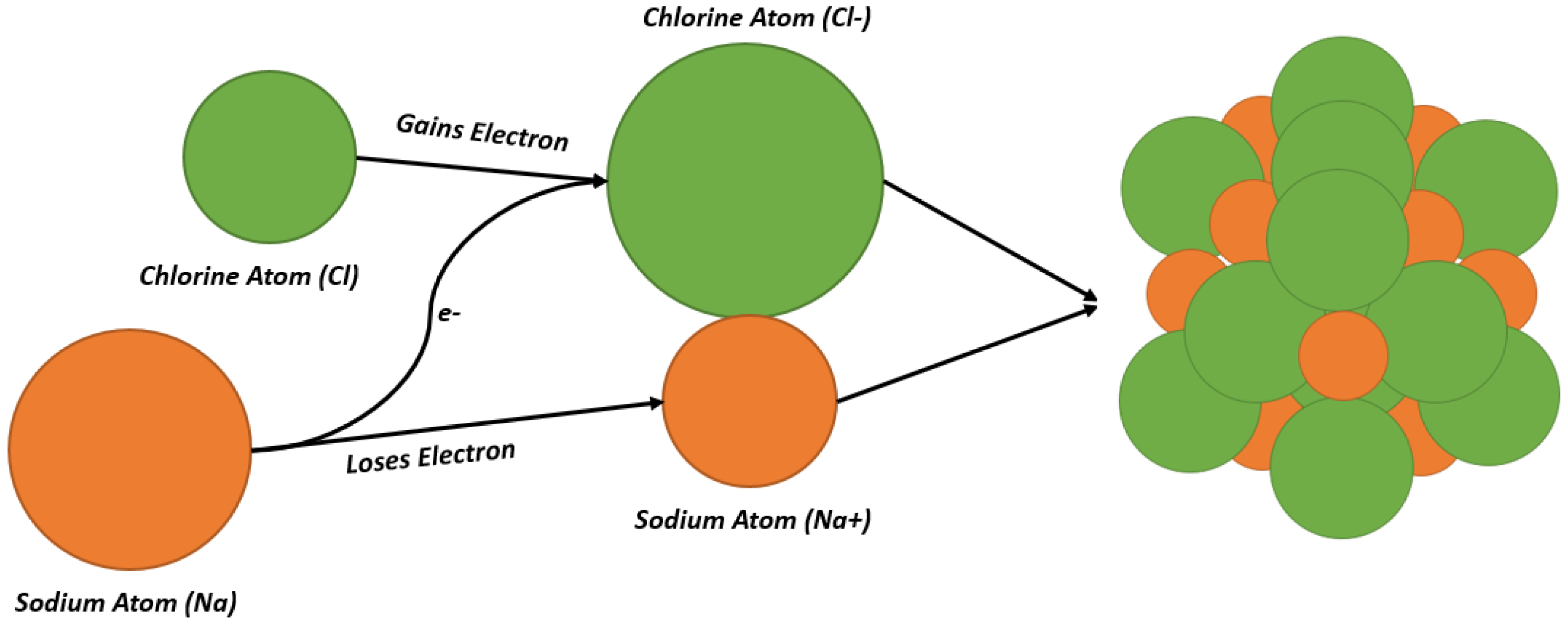
In addition, ionic compounds contain multiple ions that are held together by the electrostatic force called ionic bonding. Although these compounds are neutral in nature, they consist of some negatively- and positively-charged ions, called anions and cations, respectively. The evaporation, precipitation, or freezing of the constituent ions are the main factors in the process of producing ionic compounds. When an atom or a small group of atoms starts to lose or gain electrons, an ionic compound forms according to the ionic bonding and charged particles. As an example, the formation of sodium chloride, also known as table salt, is depicted in Figure 1. In the process of electron transformation, a sodium (neutral) becomes a sodium cation (Na+) when it loses one electron. In addition, Cl becomes a chloride anion (Cl−) when it gains an electron. Thus, table salt is a solid aggregation of Na+ and Cl− ions, which attract each other due to opposite charges.
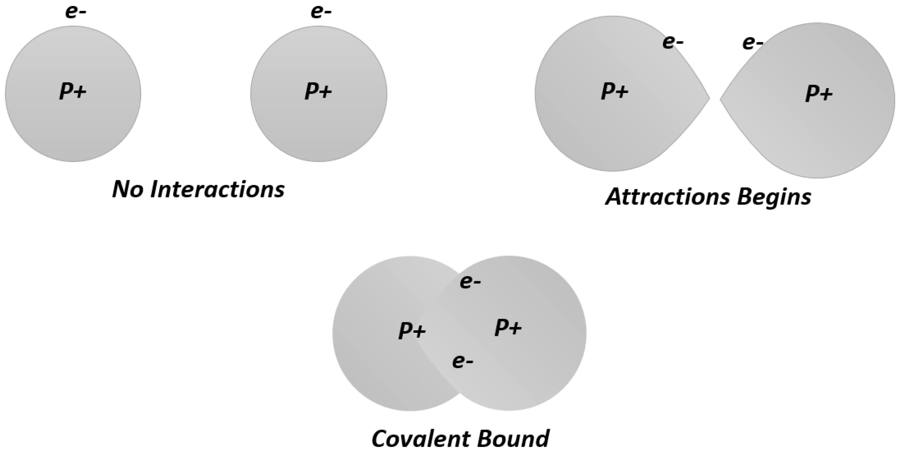
Covalent compounds form when an atom of a chemical element shares an electron with another element’s atom, which usually occurs between nonmetal elements and results in an electrically neutral atom. Figure 2 displays the formation of a covalent compound that leads to the hydrogen atom. As an example, assuming that two hydrogen atoms begin approaching each other, the nucleus of one atom strongly attracts the electron of the other one. A covalent bond is achieved when a specific distance between the nuclei is reached, and the electrons are equally shared. The net repulsion between nuclei is ignored due to the greater net attraction.
2.1.2. Chemical Reaction
Chemical reactions are the process of transforming one material into another while the chemical equations are used to represent chemical reactions, where the resulting products will have different properties than the starting materials (reactants/reagents), and intermediate materials (in some particular cases).
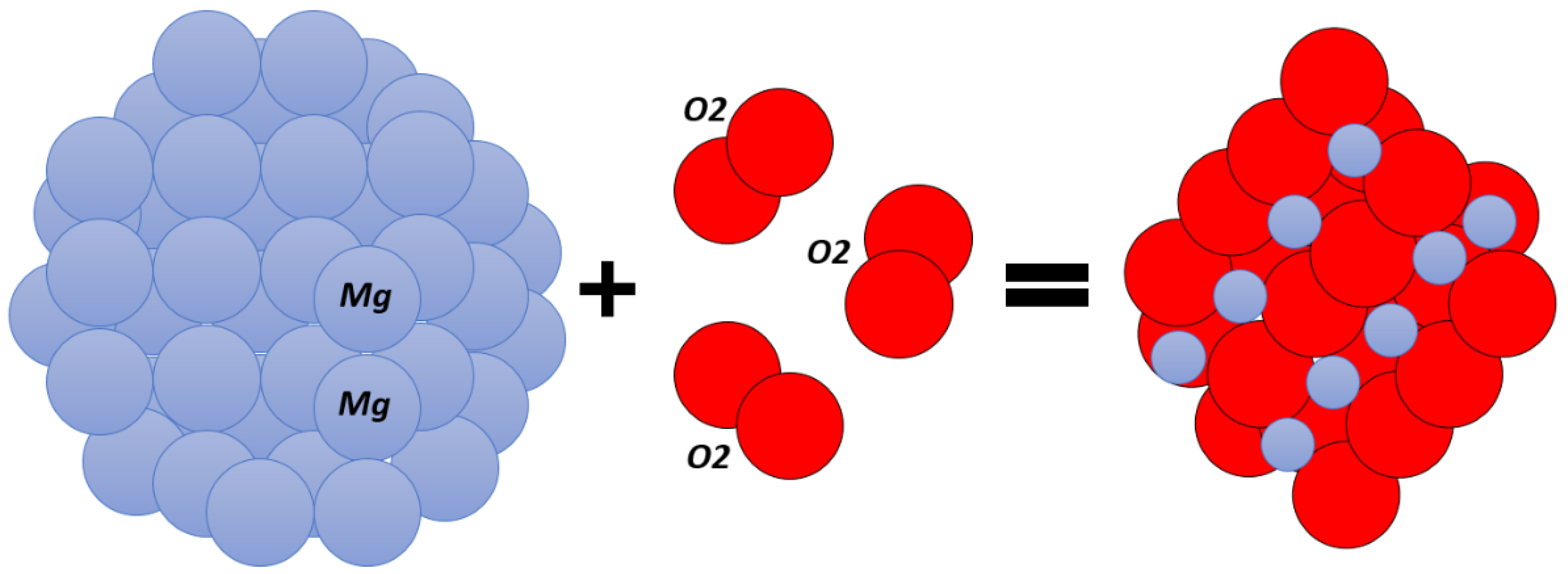
An example of a chemical reaction is depicted in Figure 3, in which the magnesium wire (Mg) and oxygen gas (O2) yield powdery magnesium oxide (MgO). As presented in the left bulb, a fine magnesium filament is surrounded by oxygen before the reaction occurs. As the reaction proceeds, the white colored powdery magnesium oxide coats the bulb’s inner surface, which is demonstrated in the right bulb. In this reaction, heat and light are also produced as intermediate materials but are not concerned in this description. The chemical equation of the presented chemical reaction is as follows:
where s and g stand for solid and gas, respectively.
2.1.3. Chemical Stability
Stability is one of the more important properties of materials in real-world applications. When generating new materials with different characteristics, it is important to consider the stability of the chemical compounds and reactions in different situations. In terms of chemical stability, chemicals have the tendency to resist changes, such as decomposition, due to internal factors and external influences such as heat, air, light, and pressure. Chemical stability is the resistance of a material to change in the presence of other chemicals. A stable chemical product refers to one that has not been specifically reactive in the environment and retains its properties over a specific period of time. Comparatively, unstable chemical materials easily decompose, corrode, polymerize, explode, or burn under certain conditions.
When producing new chemical materials, the processes of transferring or sharing electrons within the initial materials will occur in such a way that the end product will be stable and applicable during a specific period of time.
2.2. Mathematical Model
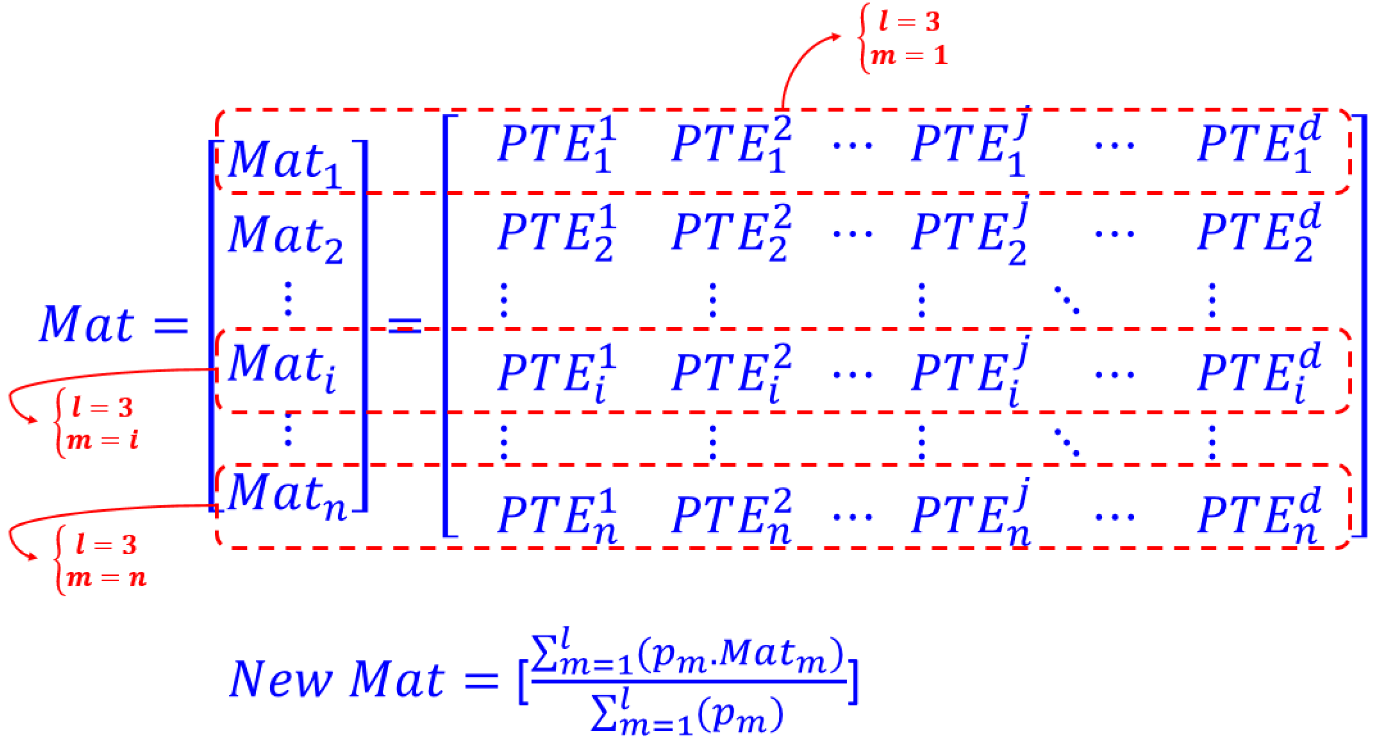
In order to conduct an optimum design procedure, an optimization algorithm is developed in this section based on the mentioned principles of material chemistry. The basic concepts of the chemical compounds, reactions, and stability are utilized in order to develop and formulate a well-defined mathematical model for the new algorithm. Considering that many natural evolution algorithms establish a predefined population of solution candidates that are evolved through random alterations and selection, MGA determines a number of materials () comprised of multiple periodic table elements (). In this algorithm, a number of materials is considered as the solution candidates (), which are comprised of some elements represented as decision variables (). The mathematical presentation of these two aspects is as follows:
where is the number of elements (decision variables) in each material (solution candidates); and is the number of materials considered to be the solution candidates.
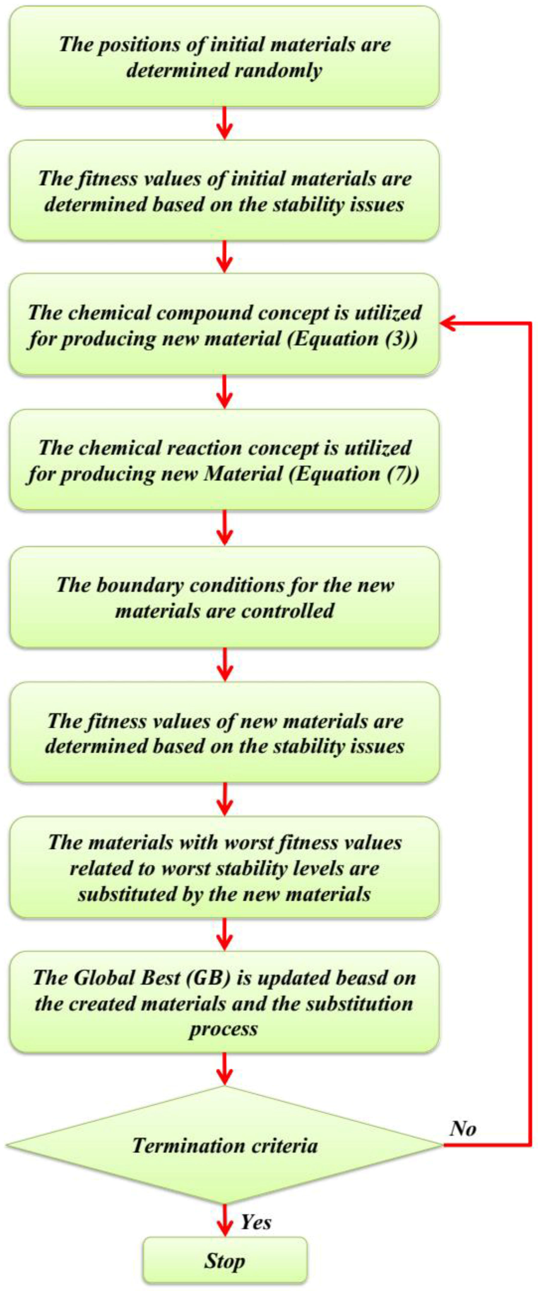
In the first stage of the optimization process, is determined randomly while the decision variables bounds are defined based on the considered problem. The initial positions of are determined randomly in the search space as follows:
where determines the initial value of the jth element in the ith material; and are the minimum allowable and maximum allowable values for the jth decision variable of the ith solution candidate, respectively; and is a random number in the interval of [0, 1].
2.2.1. Modeling Chemical Compound
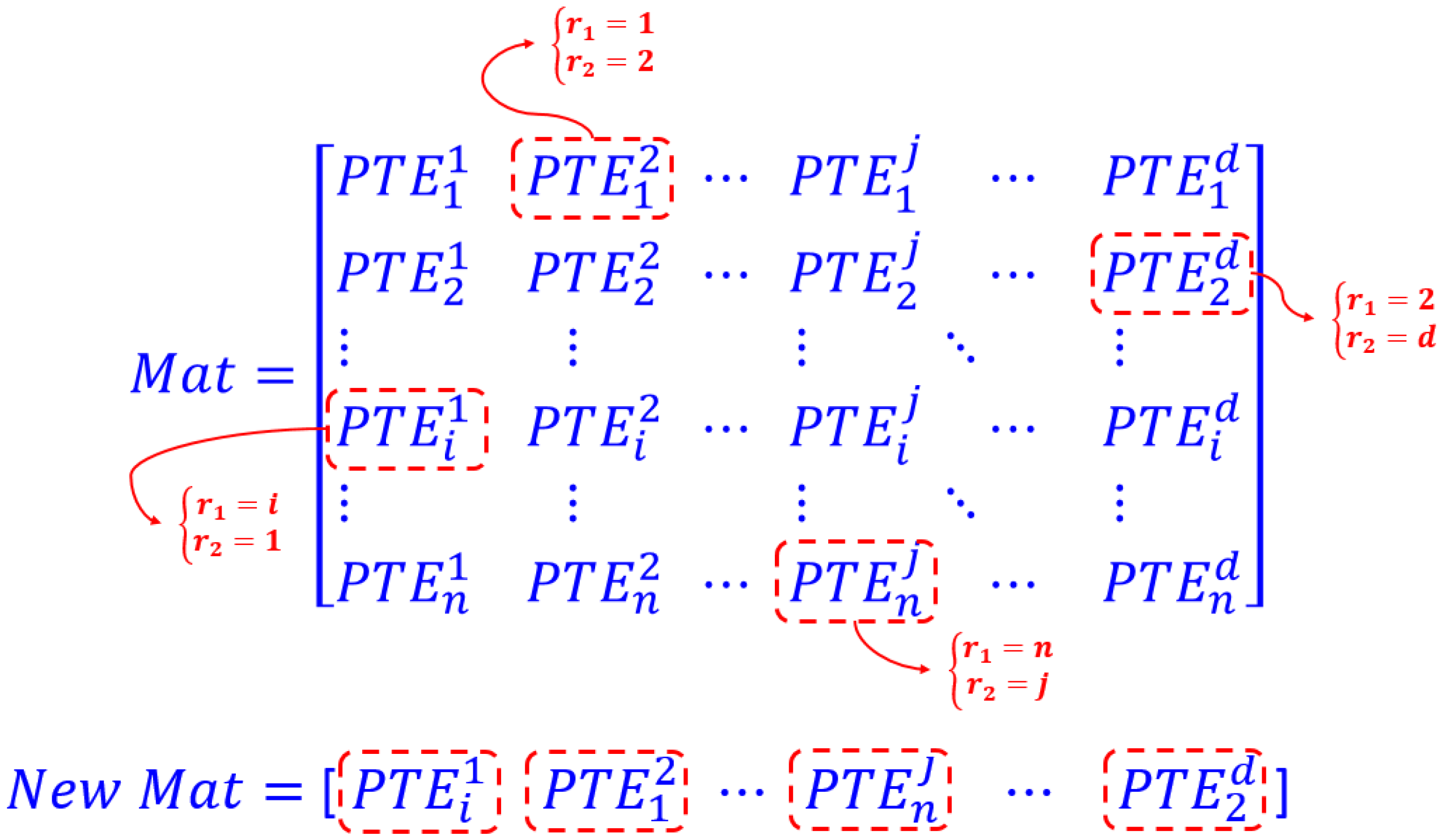
To mathematically model the chemical compounds, all are assumed to be in the ground state, which can be externally excited by the magnetic fields, absorption of energy from photons or light and interactions with different colliding bodies or particles regarding ions or other individual electrons. Due to the different stabilities of elements, they have a tendency to lose, gain, or even share electrons with other , resulting in ionic or covalent compounds. To model the ionic and covalent compounds, random are selected using the initial (Equation (1)). For the selected , the processes of losing, gaining, or sharing electrons are modeled through the probability theory. To fulfill this aim, a continuous probability distribution is utilized for each to configure a chemical compound, which is considered as a new as follows:
where and are uniformly distributed random integers in the intervals of [1, ] and [1, ], respectively; is a randomly selected from the ; is the probabilistic component for modeling the process of losing, gaining or sharing electrons represented with normal Gaussian distribution in the mathematical model; and is the new material.
The newly-created are utilized for producing a new material (), which is then added to the initial material list () as a new solution candidate:
Then, the overall solution candidates are combined and presented as follows:
A schematic presentation of the described process for the configuration of new materials based on the concept of chemical compounds (ionic and covalent) is depicted in Figure 4.
The probabilistic approach for determining is modeled through normal Gaussian distribution, which is important in statistics and often used in the natural and social sciences to represent real-valued random variables with unknown distributions. The probability of selecting a new element () regarding the randomly selected initial element () is presented as follows:
where is the mean, median or expectation of the distribution correspond to the selected random (); is the standard deviation, which is set to unity in this paper; is the variance; and is the natural base or Naperian base of the natural logarithm.
2.2.2. Modeling Chemical Reaction
Chemical reactions are sort of production process in which different chemical changes are determined in order to produce different products with modified properties even different from the initial reactants. In order to mathematically model the process of producing new materials by the chemical reaction concept, an integer random number () is determined regarding the number of materials of the initial are considered for participating in a chemical reaction. Then, integer random numbers () are generated to determine the positions of the selected materials in the initial so, the new solutions are linear combinations of the other solutions. For each material, a participation factor () is also calculated since different materials would participate in the reactions with different amounts. A schematic presentation of the described process is depicted in Figure 5, and the mathematical presentation is as follows:
where is the randomly selected material from the initial ; is the normal Gaussian distribution for the material participation factor; and is the new material produced by the chemical reaction concept.
2.2.3. Modeling Chemical Stability
As previously described, the principle of material stability concerns the tendency of natural systems to seek local and general equilibria at all structural levels. Material stability is mathematically represented by determining the quality of the solutions as . Materials with the highest stability levels alongside the ones with lowest stability levels are equivalent to the best and worst fitness values of all solution candidates in the optimization runs.
Considering the chemical compound and chemical reaction configuration approaches, the overall solution candidates are combined as follows:
Moreover, the stability levels of the initial material and newly0produced materials should be considered in order to decide whether or not the new materials should be included in the overall material list () corresponding to the solution candidates. The quality of new solution candidates is then compared to the initial ones, whereby the new materials should be substituted by initial materials with worst fitness values corresponding to worst stability levels.
For boundary violation control, a flag is determined in order to control the violating solution candidates while a maximum number of iteration or objective function evaluation can be considered as stopping criteria. The flowchart of the MGA algorithm is presented in Figure 6.
3. Problem Statement
In this section, a brief description of the considered design examples is presented. Regarding the fact that these examples are categorized as constrained optimization problems, the general formulations of these kinds of optimization problems are presented as follows:
where is considered as the objective function of the optimization problem that can be considered to be maximized or minimized; and are the ith and jth inequality and equality constraint, respectively; is the position vector related to the optimization variables; and and are the total number of inequality and equality constraints, respectively.
In most cases, the equality constraints can be transformed into inequality constraints by considering the following:
where is a predefined small positive number, which is typically near to zero. In this work, was set to 0.0001.
3.1. Mathematically-Constrained Problems
The mathematical problems of the CEC 2017 benchmark suite are presented in Table 2, while the specific details and mathematical formulations were presented in detail by Wu et al. [39]. In order to evaluate the results of the proposed MGA, the statistical results of different state-of-the-art metaheuristic algorithms regarding the considered constrained problems were derived of the recent literature [38,39,40].
3.2. Engineering Design Problems
The second type of constrained problems included 15 well-known engineering problems, which have been solved by different optimization algorithms. A brief description of these design examples is presented in Table 3, and the specific details of each example are provided in the following subsections. These examples have also been benchmarked by Kumar et al. [43] regarding the CEC 2020 engineering design scheme.
4. Numerical Results of Mathematical Problems
The numerical results based on the CEC 2017 benchmark problems by means of the MGA and other alternatives in dealing with the described constrained problems with different dimensions of 10, 30, 50, and 100 are presented in this section. For comparison, a total of 25 optimization runs was performed, including a maximum number of function evaluations (20,000 × D), where D is the problem dimension. These results are presented in Table 4, Table 5, Table 6 and Table 7 for different dimensions, in which (c) is the number of violated constraints consisting of the number of violations by more than 1, 0.01, and 0.0001; () is the mean violation at the median solution; (SR) is the feasibility rate defined as the ratio of feasible runs to total runs; and () is the mean constraint violation values of all optimization runs.
Based on the obtained results of MGA in dealing with the mathematical constrained problems of CEC 2017 with a dimension of 10, MGA was superior to the other metaheuristics in most of the cases. Considering the functions with dimensions of 30, MGA outranks two of the alternative metaheuristics while in comparing to the third one, the results of MGA are so competitive. In dealing with functions of 50 and 100 dimensions, the results of MGA are comparable to the others.
Regarding the fact that the considered problems of the CEC 2017 benchmark suite are all the latest problems in the evolutionary computation field with higher levels of complexity and difficulties while there are few approaches that can provide acceptable results in dealing with these problems. In this regard, the reported results by MGA are marginal because there are not any better results for the considered problems in the literature so the MGA calculated the latest reported results which demonstrate the capability of this algorithm in competing with other methods.
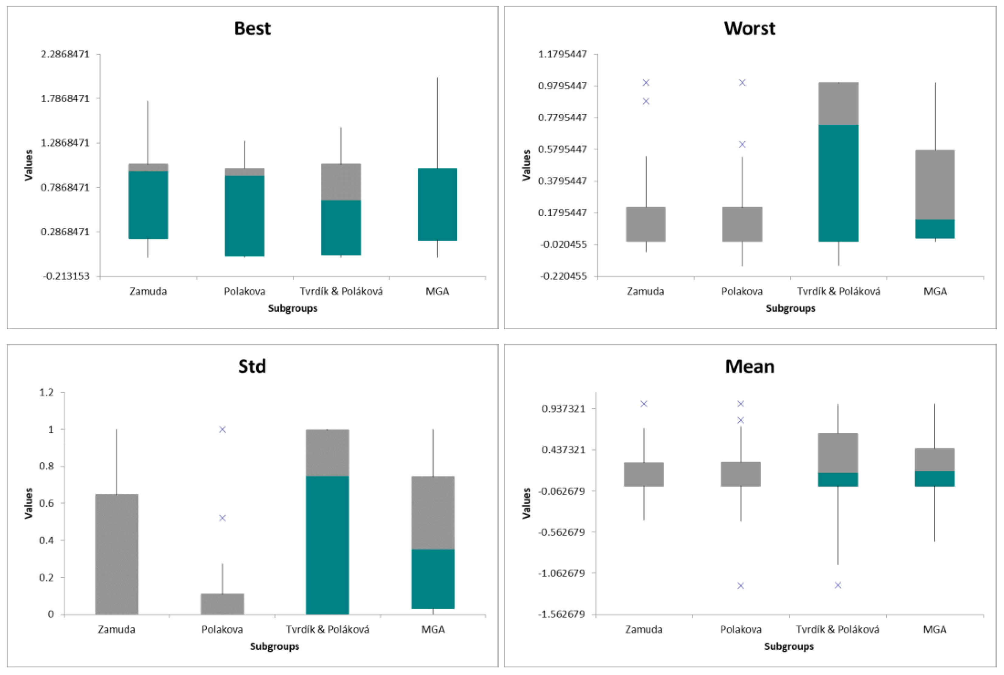
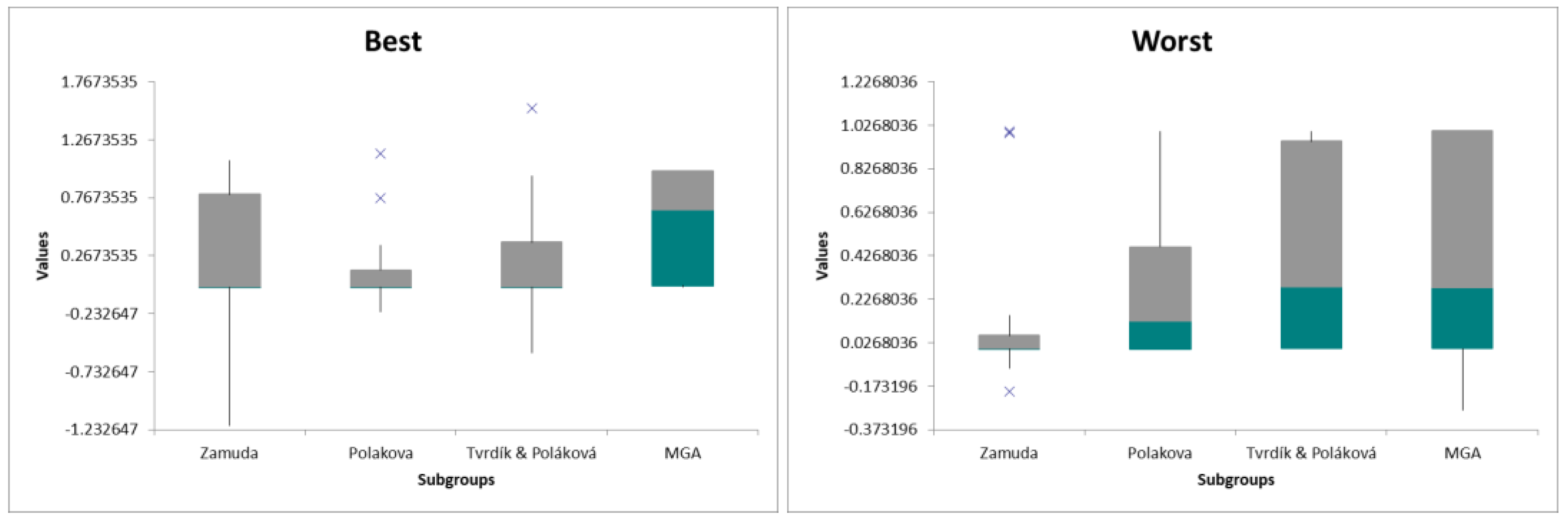
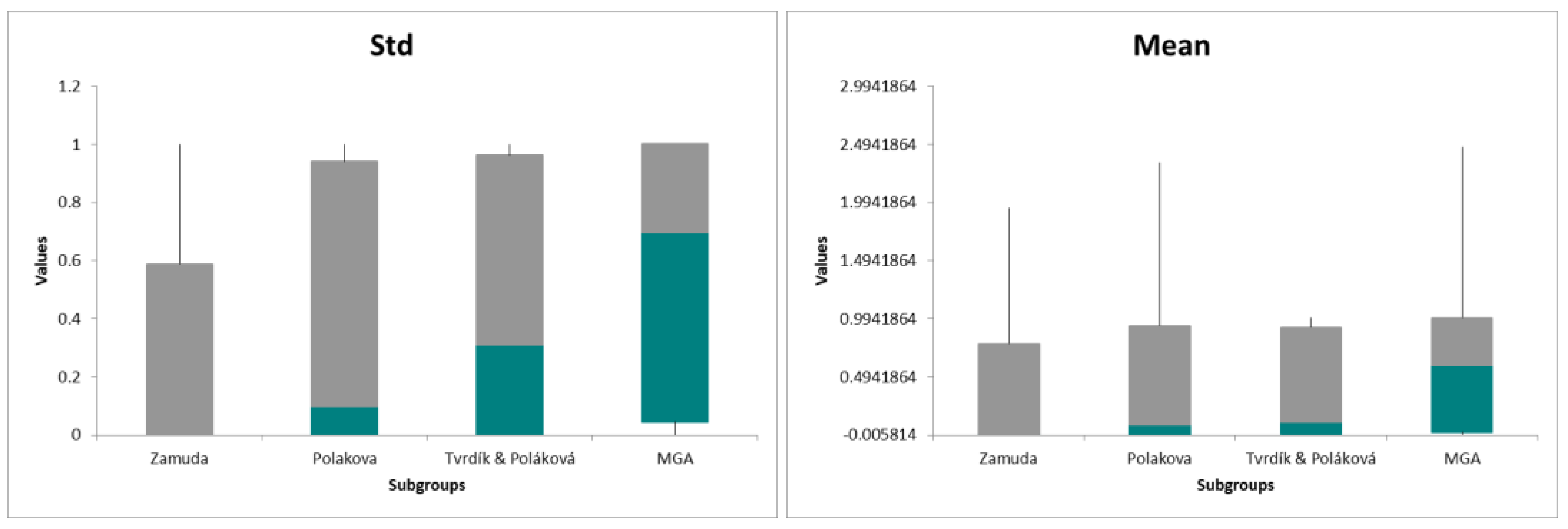
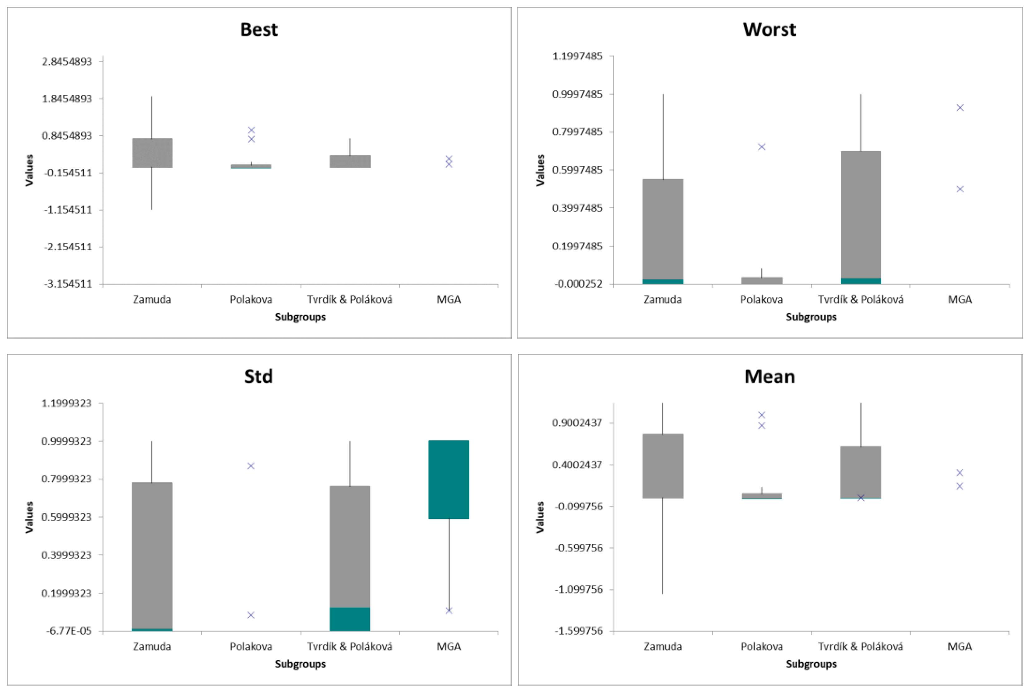
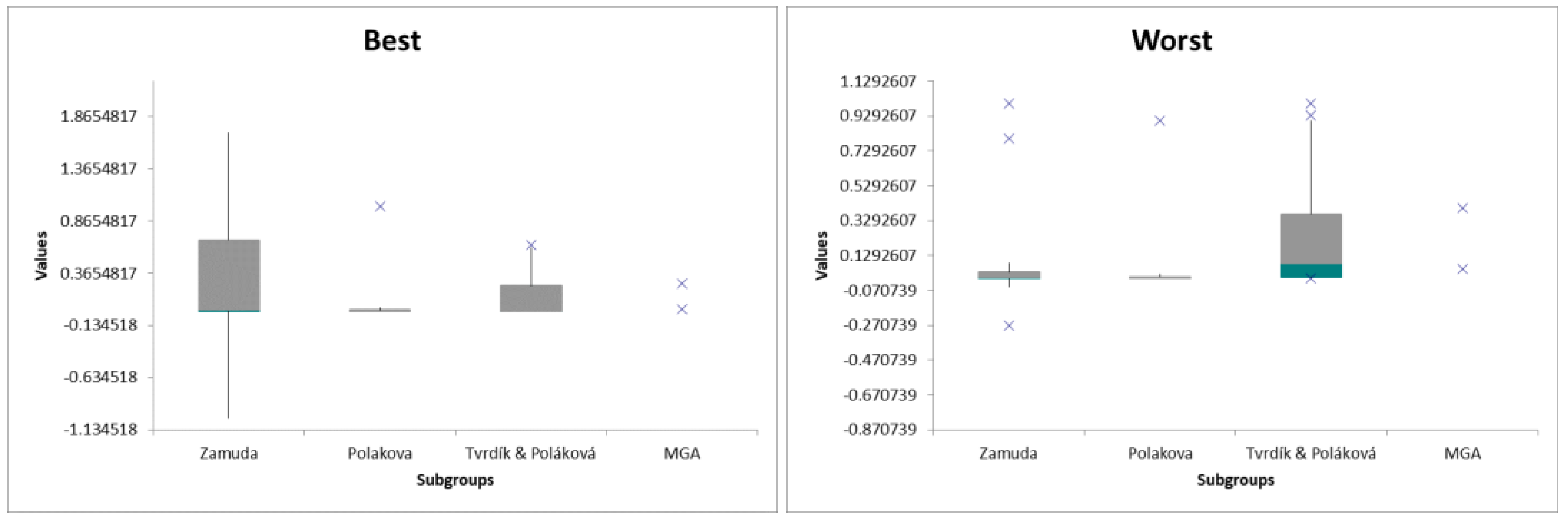
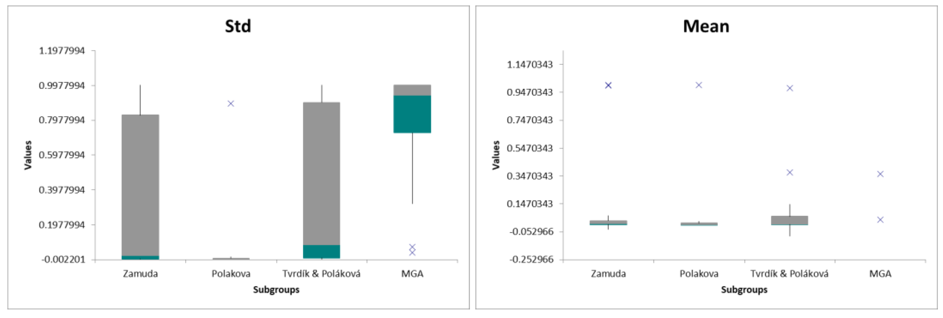
In order to have a better perspective on the performance of different metaheuristic algorithms in dealing with the CEC 2017 benchmark problems, the box plots which are derived of the analysis of the variance (ANOVA), which were conducted for the normalized values of the reported bests, means, standard deviations (Std), and worsts for different dimensions of 10, 30, 50, and 100 in Figure 7, Figure 8, Figure 9 and Figure 10. It can be concluded that the MGA has competitive performance in dealing with these problems.
Based on the provided results for the MGA and other state-of-the-art approaches in the evolutionary computation field, the AGA is capable of competing with these excellent algorithms while in some cases even MGA outperforms the others. this performance in dealing with CEC 2017 lead to the fact that MGA’s mathematical model is well-established model in which the global and local search are conducted with no need to any parameters to be tuned. In other words, this algorithm does not need any internal parameters to be defined prior to the optimization process which makes this algorithm a best choice in dealing with complex problems in which there are not any information about the complexity level of the problem. Additionally, the MGA generates only two new solution candidates in each iteration which makes the algorithm to require less computational efforts for optimization purposes. Hence, these aspects can be of great importance when the MGA is compared to the other metaheuristic algorithms in the evolutionary computation field. In other words, MGA is a parameter free optimization approach with less computational cost, which makes this algorithm different form the other approaches, while the inspirational concept of this algorithm is also unique.
5. Numerical Results of Engineering Problems
The numerical results of MGA considering the previously-described engineering design problems are presented in this section. In this regard, the results of other metaheuristics in dealing with these design examples were taken from the literature in order to make fair judgments.
The comparative results of the speed reducer design engineering problem, including the obtained design (decision) variables related to the best optimum configuration determined by different methods, are presented in Table A1. In addition, the statistical results, such as the best, mean, and worst fitness values alongside the standard deviation, are presented in Table 8. The results of different metaheuristics show that the best results of MGA are better than the best results of the other approaches in dealing with this design example. The MGA is also capable of providing better statistical results, including mean and standard deviation. The Friedman statistical test results are also presented in Table A2 for comparative purposes.
Considering the spring design problem, the best and statistical results of different metaheuristics, including the obtained design variables related to the best optimum design, are presented in Table A3 and Table 9, respectively. It should be mentioned that MGA is capable of obtaining very competitive results for this constrained engineering design problem. It also should be mentioned that MGA yields better statistical results in terms of the mean, worst fitness values alongside the standard deviation than the results of other metaheuristics. The Friedman statistical test results are also presented in Table A4 for comparative purposes.
Table A5 and Table 10 present the final and statistical results obtained by the different methods for the pressure vessel engineering design problem, respectively. From these tables, the best result of the MGA method is better than the results of the other approaches. By comparing the statistical results, it is obvious that MGA has better performance in statistical analysis, especially the mean, and worst fitness values alongside the standard deviation. The Friedman statistical test results are also presented in Table A6 for comparative purposes.
The results of the welded beam design problem in Table A7 and Table 11 show that MGA is capable of converging to better results than the other approaches. Although the maximum difference between the best results of MGA and the other approaches is only about 4%, MGA is capable of providing better statistical results, including the mean, worst fitness values alongside standard deviation. The Friedman statistical test results are also presented in Table A8 for comparative purposes.
In Table A9, the final design of different methods and MGA for the three-bar truss design problem, including the obtained design variables, are presented. Table 12 displays the statistical results. Considering the results reported by previous researchers, it is clear that MGA yields very competitive results for this engineering design problem. MGA determined the best optimum value that has been reported thus far, according to the literature, for the considered design example. It also should be noted that the statistical results, including the mean and standard deviation, for the MGA are much better than the results of other approaches. The Friedman statistical test results are also presented in Table A10 for comparative purposes.
The results of the multiple disk clutch brake design problem solved by MGA and other approaches are summarized in Table A11 [47,50,65,68]. The statistical results are presented in Table 13. Accordingly, MGA is capable of calculating very impressive results compared to the other metaheuristics. The maximum and minimum differences between the results of MGA and other metaheuristics are about 49% and 24%, which demonstrates the capability of this algorithm in dealing with multiple disk clutch brake design problem. In addition, the statistical results, including the mean and worst fitness values, demonstrate that MGA can yield extremely better results than the other approaches. The Friedman statistical test results are also presented in Table A12 for comparative purposes.
The final results of different metaheuristics in dealing with the planetary gear train design problem, one of the most important and well-established constrained optimization problems, are presented in Table A13 and Table 14. By comparing the best results of MGA with other approaches, it can be concluded that MGA can yield outstanding results. Although MGA is also capable of providing better statistical results for the mean and worst fitness values alongside standard deviation results cannot be compared since they have yet to be reported in the literature. The Friedman statistical test results are also presented in Table A14 for comparative purposes.
For the step-cone pulley engineering design problem, the final results of different metaheuristics are presented in Table A15, and the statistical results are provided in Table 15. By comparing the best results, it can be concluded that MGA can yield very impressive results for this constrained engineering problem. The maximum difference between the mean results of MGA and other approaches is about 31%. The Friedman statistical test results are also presented in Table A16 for comparative purposes.
In Table 16, the comparative results of different metaheuristics in dealing with the hydrostatic thrust bearing design problem, including the obtained design and its related best optimum configuration, are presented. Table 17 displays the statistical results. It can be concluded that MGA is capable of converging to better results than the other approaches. The maximum difference between the best results of MGA is about 29%, where MGA yielded better statistical results for the mean, worst fitness values alongside the standard deviation than the other approaches. The Friedman statistical test results are also presented in Table 18 for comparative purposes.
The optimum results of different metaheuristics in dealing with the ten-bar truss design problem are presented in Table 19 and Table 20. By comparing the best results, it can be concluded that MGA is capable of outperforming other metaheuristics approaches. Until now, the best value obtained for this example was 529.25, which has been overcome by MGA with 529.12. This indicates the capability of MGA to provide remarkable results for some complex constrained design problems.
The results of different methods for the rolling element bearing design problem are presented in Table 21 and Table 22. It is clear that the best result of the MGA in this case is better than those of other approaches in the literature. Regarding the fact that this problem is a maximization optimization problem, MGA is also capable of providing remarkable statistical results.
Table A17 [46,79,80,81] and Table 23 display the comparative and statistical optimization results of multiple optimization algorithms and MGA in dealing with the gear train design problem. It is obvious that MGA outranks the other optimization algorithms, Specifically, MGA obtained a perfect best of zero, which has not been obtained by other metaheuristics, confirming the capability of MGA to yield the lowest possible value in this case. The Friedman statistical test results are also presented in Table A18 for comparative purposes.
Considering the steel I-shaped beam as one of the most well-formulated design problems, the final and statistical optimization results of multiple metaheuristics are presented in Table 24 and Table 25, respectively. By comparing these optimum results, MGA outranked all other well-known algorithms that have been reported recently.
The final results of different metaheuristics for the piston lever design problem, a frequently occurring optimization problem, are presented in Table A19. The statistical results, including the best, mean, and worst fitness values alongside standard deviation, are presented in Table 26 for comparative purposes. Based on the results, MGA is capable of providing better statistical (mean, worst, and standard deviation of the results) and greatly outranked the other algorithms in terms of the best results. The Friedman statistical test results are also presented in Table A20 for comparative purposes.
Considering the cantilever beam engineering design problem, the optimization results of the different optimization algorithms are all presented in Table 27 and Table 28. By comparing the best results of these methods, it can be concluded that MGA is capable of achieving better results. According to the literature, recently-developed algorithms can yield 1.34, at best, for this example. Herein, we found that MGA is capable of providing even better result (1.33997) by conducting a better searching procedure. The statistical results of other optimization algorithms are not reported in the literature; thus, the remarkable results of MGA are beneficial for future works.
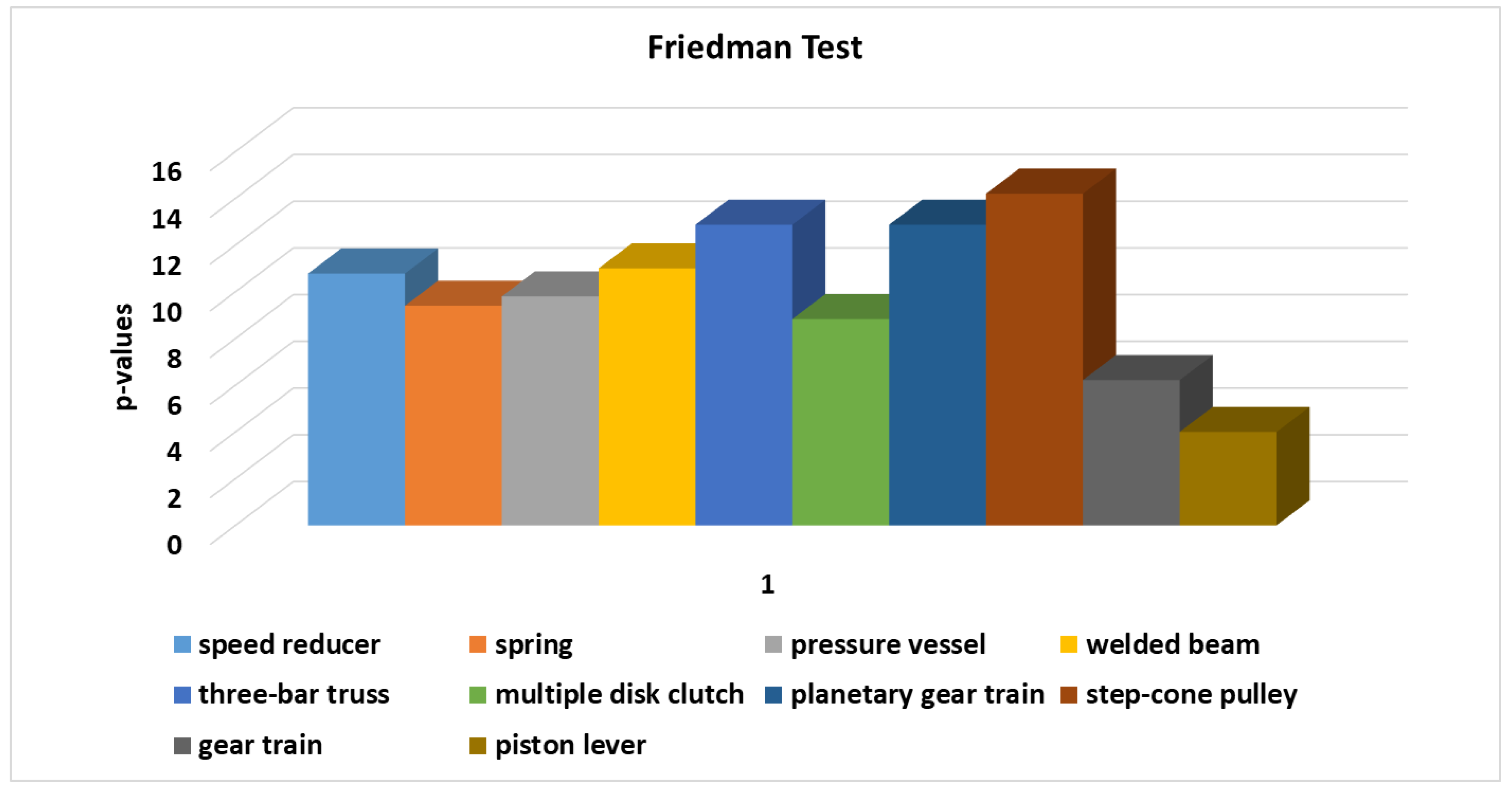
By comparing the p-values of the Friedman statistical test which are presented in the table of results by Chi-sq., it is concluded that for the piston lever design example, the lowest p-values is determined which demonstrates the fact that for this example, there are noticeable difference between the results of different approaches. However, the p-values of other examples are also near a mean of 9 which represents the stability of the conducted optimization runs and the statistical tests (Figure 11).
6. Conclusions
In this paper, the Material Generation Algorithm (MGA) is presented as a new metaheuristic for different applications and various optimization problems. In this regard, 25 constrained design problems were considered to evaluate MGA, including 10 mathematically-constrained problems presented by the Competitions on Evolutionary Computation (CEC 2017) and 15 well-known engineering design problems. For comparative purposes, the best results of different metaheuristic algorithms, such as state-of-the-art metaheuristics from CEC 2017, were selected for comparative purposes. Considering the results of MGA in dealing with the mathematical problems, it should be noted that this algorithm is capable of providing very competitive results in different dimensions. In addition, MGA yielded very impressive results in all of constrained engineering design problems compared to the previously reported algorithms. Specifically, the highest difference of about 24% between the best results of MGA and the best results reported thus far in the literature was found for the multiple disk clutch brake engineering design problem. For the three-bar truss design problem, MGA can provide very competitive results and, importantly, nearly the best results reported thus far. For the tension or compression spring, pressure vessel and rolling element bearing problems, the best results were higher for MGA than the best reported results.
While the proposed MGA has been proven to be a powerful method, different applications of this method are suggested for future research. It should be mentioned that the capability of this optimization approach can be controlled in dealing with some complex real-world and even computationally-expensive optimization problems. In addition, some other challenges, such as improving the general formulation of this method and hybridizing with other approaches, should be investigated properly.
Author Contributions
Conceptualization, S.T.; methodology, S.T. and M.A.; software, S.T. and M.A.; Validation, M.A. and S.T.; formal analysis, M.A.; investigation, S.T., M.A. and A.H.G.; resources, S.T., M.A. and A.H.G.; data curation, A.H.G.; writing—original draft preparation, M.A.; writing—review and editing, S.T. and A.H.G.; visualization, M.A.; supervision, S.T.; project administration, S.T.; funding acquisition, S.T., M.A. and A.H.G. All authors have read and agreed to the published version of the manuscript.
Funding
The APC was funded by University of Technology Sydney Internal Fund for A.H. Gandomi.
Institutional Review Board Statement
Not applicable.
Informed Consent Statement
Not applicable.
Data Availability Statement
The Matlab implementation of MGA is accessible at: www.mathworks.com/matlabcentral/fileexchange/92065-material-generation-algorithm-mga (accessed on 3 May 2021).
Acknowledgments
This research was partially supported by the University of Tabriz, grant number 1615 and the APC was funded by University of Technology Sydney Internal Fund for A.H. Gandomi.
Conflicts of Interest
The authors declare no conflict of interest.
Appendix A

Table A1.
Comparison of the best solutions for the speed reducer design problem.
| Montes et al. [54] | Akhtar et al. [55] | Gandomi et al. [46] | Zhang et al. [56] | Present Study (MGA) | |
|---|---|---|---|---|---|
| Best | 3025.005 | 3008.08 | 3000.9810 | 2994.471066 | 2994.438869 |
| b | 3.506163 | 3.506122 | 3.5015 | 3.5 | 3.500007956 |
| m | 0.700831 | 0.700006 | 0.7000 | 0.7 | 0.700000656 |
| z | 17 | 17 | 17.0000 | 17 | 17.00000081 |
| l1 | 7.460181 | 7.549126 | 7.6050 | 7.3 | 7.300541927 |
| l2 | 7.962143 | 7.85933 | 7.8181 | 7.7153199115 | 7.715357693 |
| d1 | 3.3629 | 3.365576 | 3.3520 | 3.3502146661 | 3.350542391 |
| d2 | 5.3090 | 5.289773 | 5.2875 | 5.2866544650 | 5.28665793 |
| g1(x) | −0.0777 | −0.0755 | −0.0743 | −0.0739152 | −2.155122277 |
| g2(x) | −0.2013 | −0.1994 | −0.1983 | −0.1979985 | −98.13710222 |
| g3(x) | −0.4741 | −0.4562 | −0.4349 | −0.9999967 | −1.924273761 |
| g4(x) | −0.8971 | −0.8994 | −0.9008 | −0.9999995 | −18.30969834 |
| g5(x) | −0.0110 | −0.0132 | −0.0011 | −0.6668526 | −0.000437152 |
| g6(x) | −0.0125 | −0.0017 | −0.0004 | −0.0000000 | −0.001666474 |
| g7(x) | −0.7022 | −0.7025 | −0.7025 | −0.7025000 | −28.09998829 |
| g8(x) | −0.0006 | −0.0017 | −0.0004 | −0.0000000 | −6.68 × 10⁻⁶ |
| g9(x) | −0.5831 | −0.5826 | −0.5832 | −0.5833333 | −6.999993318 |
| g10(x) | −0.0691 | −0.0796 | −0.0890 | −0.0513257 | −0.374728341 |
| g11(x) | −0.0279 | −0.0179 | −0.0130 | −0.0000000 | −3.40 × 10−05 |
Table A2.
Friedman statistical test results for the speed reducer design problem.
| Rankings | Algorithms | Mean of Ranks |
|---|---|---|
| 1 | Present Study (MGA) | 1.50 |
| 2 | Zhang et al. [56] | 2.00 |
| 3 | Gandomi et al. [46] | 3.00 |
| 4 | Akhtar et al. [55] | 3.87 |
| 5 | Montes et al. [54] | 4.62 |
| Chi-sq. | 10.7848 | |
| Prob > Chi-sq. | 0.0291 | |
Table A3.
Comparison of the best solutions for the tension or compression spring design problem.
| Coello [57] | Ray and Liew [58] | Han et al. [59] | Gandomi et al. [45] | Present Study (MGA) | |
|---|---|---|---|---|---|
| Best | 0.01270478 | 0.0126692 | 0.01266534 | 0.01266522 | 0.01266523 |
| d | 0.051480 | 0.052160 | 0.0516800 | 0.05169 | 0.051689061 |
| D | 0.351661 | 0.368159 | 0.3565001 | 0.35673 | 0.35671774 |
| N | 11.632201 | 10.648442 | 11.3018335 | 11.2885 | 11.28896576 |
| g1(x) | −0.003337 | −7.45 × 10⁻⁹ | −6.218 × 10⁻⁶ | 0 | 0 |
| g2(x) | −0.000110 | −3.68 × 10⁻⁹ | −1.691 × 10⁻⁶ | 0 | 0 |
| g3(x) | −4.026318 | −4.075805 | −4.0533150 | −4.0538 | −4.05378563 |
| g4(x) | −0.731239 | −0.719787 | −0.7278799 | −0.7277 | −0.7277288 |
Table A4.
Friedman statistical test results for the tension or compression spring design problem.
| Rankings | Algorithms | Mean of Ranks |
|---|---|---|
| 1 | Present Study (MGA) | 1.25 |
| 2 | Han et al. [59] | 2.25 |
| 3 | Coello [57] | 3.50 |
| 4 | Ray and Liew [58] | 4.00 |
| 5 | Gandomi et al. [45] | 4.00 |
| Chi-sq. | 9.4000 | |
| Prob > Chi-sq. | 0.0518 | |
Table A5.
Comparison of the best solutions for the pressure vessel design problem.
| He and Wang [60] | Coelho [61] | Mezura-Montes and Coello [62] | Coello and Montes [63] | Present Study (MGA) | |
|---|---|---|---|---|---|
| Best | 6061.0777 | 6059.7208 | 6059.7456 | 6059.9463 | 6059.714350 |
| Ts | 0.8125 | 0.8125 | 0.8125 | 0.8125 | 0.8125 |
| Th | 0.4375 | 0.4375 | 0.4375 | 0.4375 | 0.4375 |
| R | 42.0913 | 42.0984 | 42.098087 | 42.097398 | 42.0984 |
| L | 176.7465 | 176.6372 | 176.640518 | 176.654050 | 176.6366 |
| g1(x) | −1.37 × 10⁻⁶ | −8.79 × 10⁻⁷ | −6.92 × 10⁻⁶ | −2.02 × 10⁻⁵ | 0 |
| g2(x) | −3.59 × 10⁻⁴ | −3.58 × 10⁻² | −0.03588 | −0.03589 | −0.0359 |
| g3(x) | −118.7687 | −0.2179 | 2.903372 | −24.8998 | 0 |
| g4(x) | −63.2535 | −63.3628 | −63.3595 | −63.346 | −63.3634 |
Table A6.
Friedman statistical test results for the pressure vessel design problem.
| Rankings | Algorithms | Mean of Ranks |
|---|---|---|
| 1 | Present Study (MGA) | 1 |
| 2 | He and Wang [60] | 2.75 |
| 3 | Coello and Montes [63] | 3.25 |
| 4 | Coelho [61] | 4.00 |
| 5 | Mezura-Montes and Coello [62] | 4.00 |
| Chi-sq. | 9.8000 | |
| Prob > Chi-sq. | 0.0439 | |
Table A7.
Comparison of the best solutions for the welded beam design problem.
| Huang et al. [64] | Eskandar et al. [65] | Guedria [66] | Han et al. [59] | Present Study (MGA) | |
|---|---|---|---|---|---|
| Best | 1.733461 | 1.724856 | 1.724852 | 1.6956397 | 1.672966512 |
| h | 0.203137 | 0.205728 | 0.205730 | 0.20532536 | 0.198957505 |
| l | 3.542998 | 3.470522 | 3.470489 | 3.26035648 | 3.341955765 |
| t | 9.033498 | 9.036620 | 9.036624 | 9.03664424 | 9.187291977 |
| b | 0.206179 | 0.205729 | 0.205730 | 0.20572991 | 0.199190532 |
| g1(x) | −44.57856 | −0.034128 | −1.05 × 10⁻¹⁰ | −0.10520197 | −20.76244473 |
| g2(x) | −44.66353 | −3.49 × 10⁻⁵ | −6.91 × 10⁻¹⁰ | −0.17417862 | −23.09392302 |
| g3(x) | −0.003042 | −1.19 × 10⁻⁶ | −7.66 × 10⁻¹⁵ | −4.04330102 | −0.000233027 |
| g4(x) | −3.423726 | −3.432980 | −3.432984 | −3.45179021 | −3.469028817 |
| g5(x) | −0.078137 | −0.080728 | −0.080730 | −0.08032536 | −0.073957505 |
| g6(x) | −0.235557 | −0.235540 | −0.235540 | −0.22831066 | −0.05415088 |
| g7(x) | −38.02826 | −0.013503 | −5.80 × 10⁻¹⁰ | −0.03397937 | −30.47032014 |
Table A8.
Friedman statistical test results for the welded beam design problem.
| Rankings | Algorithms | Mean of Ranks |
|---|---|---|
| 1 | Present Study (MGA) | 1.50 |
| 2 | Guedria [66] | 2.25 |
| 3 | Han et al. [59] | 3.25 |
| 4 | Eskandar et al. [65] | 3 |
| 5 | Huang et al. [64] | 5 |
| Chi-sq. | 11.0000 | |
| Prob > Chi-sq. | 0.0266 | |
Table A9.
Comparison of the best solutions for the three-bar truss design problem.
| Gandomi et al. [46] | Ray and Liew [58] | Zhang et al. [56] | Grag [67] | Present Study (MGA) | |
|---|---|---|---|---|---|
| Best | 263.97156 | 263.8958466 | 263.8958434 | 263.8958433 | 263.8958433 |
| A1 | 0.78867 | 0.7886210370 | 0.7886751359 | 0.788676171219 | 0.788675136 |
| A2 | 0.40902 | 0.4084013340 | 0.4082482868 | 0.408245358456 | 0.408248288 |
| g1(x) | −0.00029 | −8.275 × 10⁻⁹ | −2.104 × 10⁻¹¹ | −1.587 × 10⁻¹³ | 0 |
| g2(x) | −0.00029 | −1.46392765 | −1.46410161 | −1.4641049 | −1.464101618 |
| g3(x) | −0.73176 | −0.536072358 | −0.5358983 | −0.535895 | −0.535898382 |
Table A10.
Friedman statistical test results for the three-bar truss design problem.
| Rankings | Algorithms | Mean of Ranks |
|---|---|---|
| 1 | Present Study (MGA) | 1.75 |
| 2 | Grag [67] | 1.87 |
| 3 | Zhang et al. [56] | 2.37 |
| 4 | Ray and Liew [58] | 4.25 |
| 5 | Gandomi et al. [46] | 4.75 |
| Chi-sq. | 12.8700 | |
| Prob > Chi-sq. | 0.0119 | |
Table A11.
Comparison of the best solutions for the multiple disk clutch brake design problem.
| Deb and Srinivasan [68] | Eskandar et al. [65] | Rao et al. [50] | Ferreira et al. [47] | Present Study (MGA) | |
|---|---|---|---|---|---|
| Best | 0.4704 | 0.313656 | 0.313656611 | 0.313656 | 0.235242467 |
| r1 | 70 | 70 | 70 | 70 | 70.00000008 |
| r0 | 90 | 90 | 90 | 90 | 90.0000003 |
| t | 1.5 | 1 | 1 | 1 | 1.000000013 |
| F | 1000 | 910 | 810 | 830 | 865.6907633 |
| Z | 3 | 3 | 3 | 3 | 2.00000004 |
| g1(x) | 0 | 0 | 0 | 0 | −2.18 × 10⁻⁷ |
| g2(x) | −22 | −24 | −24 | −24 | −25.4999999 |
| g3(x) | −0.9005 | −0.909480 | −0.91942781 | −0.917438 | −0.913888149 |
| g4(x) | −9.7906 | −9.809429 | −9830.371094 | −9.826183 | −9.985383395 |
| g5(x) | −7.8947 | −7.894696 | −7894.69659 | −7.894697 | −9.830260243 |
| g6(x) | −3.3527 | −2.231421 | −0.702013203 | −0.173855 | −14.98276443 |
| g7(x) | −60.6250 | −49.768749 | −37706.25 | −40.118750 | −83479.16052 |
| g8(x) | −11.6473 | −12.768578 | −14.2979868 | −14.826145 | −0.017235569 |
Table A12.
Friedman statistical test results for the multiple disk clutch brake design problem.
| Rankings | Algorithms | Mean of Ranks |
|---|---|---|
| 1 | Present Study (MGA) | 1.5 |
| 2 | Ferreira et al. [47] | 2.12 |
| 3 | Eskandar et al. [65] | 2.37 |
| 4 | Rao et al. [50] | 4.00 |
| Chi-sq. | 8.8378 | |
| Prob > Chi-sq. | 0.0315 | |
Table A13.
Comparison of the best solutions for the planetary gear train design problem.
| Savsani and Savsani [48] | Present Study (MGA) | |
|---|---|---|
| Best | 0.525588 | 0.52325 |
| N1 | 34 | 40 |
| N2 | 25 | 21 |
| N3 | 33 | 14 |
| N4 | 32 | 19 |
| N5 | 23 | 17 |
| N6 | 116 | 69 |
| P | 4 | 3 |
| m1 | 2.5 | 2 |
| m2 | 1.75 | 3 |
Table A14.
Friedman statistical test results for the planetary gear train design problem.
| Rankings | Algorithms | Mean of Ranks |
|---|---|---|
| 1 | Present Study (MGA) | 2.50 |
| 2 | Zhang et al. [70] | 2.50 |
| 3 | Savsani and Savsani [48] | 3.00 |
| 4 | Rao and Savsani [69] (ABC) | 3.00 |
| 5 | Rao and Savsani [69] (PSO) | 4.00 |
| Chi-sq. | 12.8700 | |
| Prob > Chi-sq. | 0.0119 | |
Table A15.
Comparison of the best solutions for the step-cone pulley design problem.
| TLBO [50] | WOA [44] | WCA [44] | MBA [44] | Present Study (MGA) | |
|---|---|---|---|---|---|
| Best | 16.63451 | 16.6345213 | 16.63450849 | 16.6345078 | 16.18595608 |
| d1 | 40 | 40 | 40 | 40 | 38.53034981 |
| d2 | 54.7643 | 54.764326 | 54.764300 | 54.764300 | 53.04151483 |
| d3 | 73.01318 | 54.764326 | 54.764300 | 54.764300 | 70.67294075 |
| d4 | 73.01318 | 54.764326 | 54.764300 | 88.428419 | 84.71470998 |
| w | 73.01318 | 85.986297 | 54.764300 | 85.986242 | 90 |
WOA: Whale Optimization Algorithm; WCA: Water Cycle Algorithm; MBA: Mine Blast Algorithm.
Table A16.
Friedman statistical test results for the step-cone pulley design problem.
| Rankings | Algorithms | Mean of Ranks |
|---|---|---|
| 1 | Present Study (MGA) | 1.00 |
| 2 | MBA [44] | 2.00 |
| 3 | WCA [44] | 3.25 |
| 4 | TLBO [50] | 4.25 |
| 5 | WOA [44] | 4.50 |
| Chi-sq. | 14.2000 | |
| Prob > Chi-sq. | 0.0067 | |
Table A17.
Comparison of the best solutions for the gear train design problem.
| Gandomi et al. [46] | Loh and Papalambros [79] | Kannan and Kramer [80] | Sandgren [81] | Present Study (MGA) | |
|---|---|---|---|---|---|
| Best | 2.701 × 10⁻¹² | 2.7× 10⁻¹² | 2.146 × 10⁻⁸ | 5.712 × 10⁻⁶ | 1.06 × 10⁻¹⁹ |
| zd | 19 | 19 | 13 | 18 | 27.32076302 |
| zb | 16 | 16 | 15 | 22 | 13.75530503 |
| za | 43 | 43 | 33 | 45 | 48.25305913 |
| zf | 49 | 49 | 41 | 60 | 53.98015133 |
Table A18.
Friedman statistical test results for the gear train design problem.
| Rankings | Algorithms | Mean of Ranks |
|---|---|---|
| 1 | Present Study (MGA) | 2.00 |
| 2 | Wang et al. [82] (CPKH) | 2.37 |
| 3 | Loh and Papalambros [79] | 2.75 |
| 4 | Wang et al. [82] (ABC) | 3.37 |
| 5 | Gandomi et al. [46] | 4.50 |
| Chi-sq. | 6.2278 | |
| Prob > Chi-sq. | 0.1828 | |
Table A19.
Comparison of the best solutions for the piston lever design problem.
| CSA [46] | Present Study (MGA) | |
|---|---|---|
| Best | 8.4271 | 8.413406652 |
| H | 0.05 | 0.05 |
| B | 2.043 | 2.041637535 |
| X | 120 | 120 |
| D | 4.0851 | 4.083080224 |
References
- Glover, F. Future paths for integer programming and links to artificial intelligence. Comput. Oper. Res. 1986, 13, 533–549. [Google Scholar] [CrossRef]
- Sörensen, K.; Sevaux, M.; Glover, F. A History of Metaheuristics; Handbook of heuristics. arXiv 2017, arXiv:1704.00853. [Google Scholar]
- Moscato, P. On Evolution, Search, Optimization, Genetic Algorithms and Martial Arts: Towards Memetic Algorithms. Caltech Concurr. Comput. Program C3P Rep. 1989, 826, 1989. [Google Scholar]
- Holland, J.H. Adaptation in Natural and Artificial Systems: An Introductory Analysis with Applications to Biology, Control, and Artificial Intelligence; MIT Press: Cambridge, MA, USA, 1992. [Google Scholar]
- Koza, J.R.; Koza, J.R. Genetic Programming: On the Programming of Computers by Means of Natural Selection; MIT Press: Cambridge, MA, USA, 1992. [Google Scholar]
- Storn, R.; Price, K. Differential evolution—A simple and efficient heuristic for global optimization over continuous spaces. J. Glob. Optim. 1997, 11, 341–359. [Google Scholar] [CrossRef]
- Beyer, H.G.; Schwefel, H.P. Evolution strategies—A comprehensive introduction. Nat. Comput. 2002, 1, 3–52. [Google Scholar] [CrossRef]
- Simon, D. Biogeography-based optimization. IEEE Trans. Evol. Comput. 2008, 12, 702–713. [Google Scholar] [CrossRef] [Green Version]
- Eberhart, R.; Kennedy, J. A New Optimizer Using Particle Swarm Theory. In Proceedings of the Sixth International Symposium on Micro Machine and Human Science, Nagoya, Japan, 4–6 October 1995; pp. 39–43. [Google Scholar]
- Dorigo, M.; Maniezzo, V.; Colorni, A. Ant system: Optimization by a colony of cooperating agents. IEEE Trans. Syst. Man Cybern. Part B Cybern. 1996, 26, 29–41. [Google Scholar] [CrossRef] [PubMed] [Green Version]
- Basturk, B. An artificial bee colony (ABC) algorithm for numeric function optimization. In Proceedings of the IEEE Swarm Intelligence Symposium, Indianapolis, IN, USA, 12 May 2006. [Google Scholar]
- Chu, S.C.; Tsai, P.W.; Pan, J.S. Cat Swarm Optimization. In Pacific Rim International Conference on Artificial Intelligence; Springer: Berlin/Heidelberg, Germany, 2006; pp. 854–858. [Google Scholar]
- Yang, X.S. Nature-Inspired Metaheuristic Algorithms; Luniver Press: Bristol, UK, 2010. [Google Scholar]
- Gandomi, A.H.; Alavi, A.H. Krill herd: A new bio-inspired optimization algorithm. Commun. Nonlinear Sci. Numer. Simul. 2012, 17, 4831–4845. [Google Scholar] [CrossRef]
- Kirkpatrick, S.; Gelatt, C.D.; Vecchi, M.P. Optimization by simulated annealing. Science 1983, 220, 671–680. [Google Scholar] [CrossRef]
- Geem, Z.W.; Kim, J.H.; Loganathan, G.V. A new heuristic optimization algorithm: Harmony search. Simulation 2001, 76, 60–68. [Google Scholar] [CrossRef]
- Erol, O.K.; Eksin, I. A new optimization method: Big bang–big crunch. Adv. Eng. Softw. 2006, 37, 106–111. [Google Scholar] [CrossRef]
- Rashedi, E.; Nezamabadi-Pour, H.; Saryazdi, S. GSA: A gravitational search algorithm. Inf. Sci. 2009, 179, 2232–2248. [Google Scholar] [CrossRef]
- Kaveh, A.; Talatahari, S. A novel heuristic optimization method: Charged system search. Acta Mech. 2010, 213, 267–289. [Google Scholar] [CrossRef]
- Alatas, B. ACROA: Artificial chemical reaction optimization algorithm for global optimization. Expert Syst. Appl. 2011, 38, 13170–13180. [Google Scholar] [CrossRef]
- Kaveh, A.; Mahdavi, V.R. Colliding bodies optimization: A novel meta-heuristic method. Comput. Struct. 2014, 139, 18–27. [Google Scholar] [CrossRef]
- Talatahari, S.; Azizi, M. Chaos Game Optimization: A novel metaheuristic algorithm. Artif. Intell. Rev. 2020, 22, 1–88. [Google Scholar] [CrossRef]
- Talatahari, S.; Azizi, M. Optimization of Constrained Mathematical and Engineering Design Problems Using Chaos Game Optimization. Comput. Ind. Eng. 2020, 145, 106560. [Google Scholar] [CrossRef]
- Azizi, M. Atomic orbital search: A novel metaheuristic algorithm. Appl. Math. Model. 2021, 93, 657–683. [Google Scholar] [CrossRef]
- Atashpaz-Gargari, E.; Lucas, C. Imperialist competitive algorithm: An algorithm for optimization inspired by imperialistic competition. In Proceedings of the 2007 IEEE Congress on Evolutionary Computation, Singapore, 25–28 September 2007; pp. 4661–4667. [Google Scholar]
- Yang, X.S.; Deb, S. Cuckoo search via Lévy flights. In Proceedings of the 2009 World Congress on Nature & Biologically Inspired Computing (NaBIC), Coimbatore, India, 9–11 December 2009; pp. 210–214. [Google Scholar]
- Talatahari, S.; Azizi, M. Tribe-charged system search for global optimization. Appl. Math. Model. 2021, 93, 115–133. [Google Scholar] [CrossRef]
- Carbas, S. Design optimization of steel frames using an enhanced firefly algorithm. Eng. Optim. 2016, 48, 2007–2025. [Google Scholar] [CrossRef]
- Hasançebi, O.; Çarbaş, S.; Saka, M.P. Improving the performance of simulated annealing in structural optimization. Struct. Multidiscip. Optim. 2010, 41, 189–203. [Google Scholar] [CrossRef]
- Azad, S.K. Design optimization of real-size steel frames using monitored convergence curve. Struct. Multidiscip. Optim. 2021, 63, 267–288. [Google Scholar] [CrossRef]
- Akış, T.; Azad, S.K. Structural Design Optimization of Multi-layer Spherical Pressure Vessels: A Metaheuristic Approach. Iran. J. Sci. Technol. Trans. Mech. Eng. 2019, 43, 75–90. [Google Scholar] [CrossRef]
- Tubishat, M.; Idris, N.; Shuib, L.; Abushariah, M.A.; Mirjalili, S. Improved Salp Swarm Algorithm based on opposition based learning and novel local search algorithm for feature selection. Expert Syst. Appl. 2020, 145, 113–122. [Google Scholar] [CrossRef]
- Mokeddem, D.; Mirjalili, S. Improved Whale Optimization Algorithm applied to design PID plus second-order derivative controller for automatic voltage regulator system. J. Chin. Inst. Eng. 2020, 43, 541–552. [Google Scholar] [CrossRef]
- Kaveh, A.; Hosseini, S.M.; Zaerreza, A. Improved Shuffled Jaya algorithm for sizing optimization of skeletal structures with discrete variables. In Structures; Elsevier: Amsterdam, The Netherlands, 2021; pp. 107–128. [Google Scholar]
- Ebrahimi, B.; Tavana, M.; Toloo, M.; Charles, V. A novel mixed binary linear DEA model for ranking decision-making units with preference information. Comput. Ind. Eng. 2020, 149, 106720. [Google Scholar] [CrossRef]
- Azizi, M.; Ghasemi, S.A.; Ejlali, R.E.; Talatahari, S. Optimization of Fuzzy Controller for Nonlinear Buildings with Improved Charged System Search. Struct. Eng. Mech. 2020, 76, 781. [Google Scholar]
- Wu, G.; Mallipeddi, R.; Suganthan, P.N. Problem Definitions and Evaluation Criteria for the CEC 2017 Competition on Constrained Real-Parameter Optimization; Technical Report; National University of Defense Technology: Changsha, China; Kyungpook National University: Daegu, Korea; Nanyang Technological University: Singapore, 2017. [Google Scholar]
- Tvrdík, J.; Poláková, R. Simple framework for constrained problems with application of L-SHADE44 and IDE. In Proceedings of the 2017 IEEE Congress on Evolutionary Computation (CEC), Donostia, Spain, 5 June 2017; pp. 1436–1443. [Google Scholar]
- Polakova, R. L-SHADE with competing strategies applied to constrained optimization. In Proceedings of the 2017 IEEE Congress on Evolutionary Computation (CEC), Donostia, Spain, 5 June 2017; pp. 1683–1689. [Google Scholar]
- Zamuda, A. Adaptive constraint handling and success history differential evolution for CEC 2017 constrained real-parameter optimization. In Proceedings of the 2017 IEEE Congress on Evolutionary Computation (CEC), Donostia, Spain, 5 June 2017; pp. 2443–2450. [Google Scholar]
- Derrac, J.; García, S.; Molina, D.; Herrera, F. A practical tutorial on the use of nonparametric statistical tests as a methodology for comparing evolutionary and swarm intelligence algorithms. Swarm Evol. Comput. 2011, 1, 3–18. [Google Scholar] [CrossRef]
- Sörensen, K. Metaheuristics—The metaphor exposed. Int. Trans. Oper. Res. 2015, 22, 3–18. [Google Scholar] [CrossRef]
- Kumar, A.; Wu, G.; Ali, M.Z.; Mallipeddi, R.; Suganthan, P.N.; Das, S. A test-suite of non-convex constrained optimization problems from the real-world and some baseline results. Swarm Evol. Comput. 2020, 56, 100693. [Google Scholar] [CrossRef]
- Yildiz, A.R.; Abderazek, H.; Mirjalili, S. A Comparative Study of Recent Non-traditional Methods for Mechanical Design Optimization. Arch. Comput. Methods Eng. 2020, 27, 1031–1048. [Google Scholar] [CrossRef]
- Gandomi, A.H.; Yang, X.S.; Alavi, A.H.; Talatahari, S. Bat algorithm for constrained optimization tasks. Neural Comput. Appl. 2013, 22, 1239–1255. [Google Scholar] [CrossRef]
- Gandomi, A.H.; Yang, X.S.; Alavi, A.H. Cuckoo search algorithm: A metaheuristic approach to solve structural optimization problems. Eng. Comput. 2013, 29, 17–35. [Google Scholar] [CrossRef]
- Ferreira, M.P.; Rocha, M.L.; Neto, A.J.; Sacco, W.F. A constrained ITGO heuristic applied to engineering optimization. Expert Syst. Appl. 2018, 110, 106–124. [Google Scholar] [CrossRef]
- Savsani, P.; Savsani, V. Passing vehicle search (PVS): A novel metaheuristic algorithm. Appl. Math. Model. 2016, 40, 3951–3978. [Google Scholar] [CrossRef]
- Rao, S.S. Engineering Optimization: Theory and Practice; John Wiley & Sons: Hoboken, NJ, USA, 2019. [Google Scholar]
- Rao, R.V.; Savsani, V.J.; Vakharia, D.P. Teaching–learning-based optimization: A novel method for constrained mechanical design optimization problems. Comput. Aided Des. 2011, 43, 303–315. [Google Scholar] [CrossRef]
- Yu, Z.; Xu, T.; Cheng, P.; Zuo, W.; Liu, X.; Yoshino, T. Optimal Design of Truss Structures with Frequency Constraints Using Interior Point Trust Region Method. Proc. Rom. Acad. Ser. 2014, 15, 165–173. [Google Scholar]
- Gupta, S.; Tiwari, R.; Nair, S.B. Multi-objective design optimisation of rolling bearings using genetic algorithms. Mech. Mach. Theory 2007, 42, 1418–1443. [Google Scholar] [CrossRef]
- Zelinka, I.; Lampinen, J. Mechanical Engineering Problem Optimization by SOMA. In New Optimization Techniques in Engineering; Springer: Berlin/Heidelberg, Germany, 2004; pp. 633–653. [Google Scholar]
- Mezura-Montes, E.; Coello, C.C.; Landa-Becerra, R. Engineering Optimization Using Simple Evolutionary Algorithm. In Proceedings of the 15th IEEE International Conference on Tools with Artificial Intelligence, Sacramento, CA, USA, 5 November 2003; pp. 149–156. [Google Scholar]
- Akhtar, S.; Tai, K.; Ray, T. A socio-behavioural simulation model for engineering design optimization. Eng. Optim. 2002, 34, 341–354. [Google Scholar] [CrossRef]
- Zhang, M.; Luo, W.; Wang, X. Differential evolution with dynamic stochastic selection for constrained optimization. Inf. Sci. 2008, 178, 3043–3074. [Google Scholar] [CrossRef]
- Coello, C.A. Use of a self-adaptive penalty approach for engineering optimization problems. Comput. Ind. 2000, 41, 113–127. [Google Scholar] [CrossRef]
- Ray, T.; Liew, K.M. Society and civilization: An optimization algorithm based on the simulation of social behavior. IEEE Trans. Evol. Comput. 2003, 7, 386–396. [Google Scholar] [CrossRef]
- Han, J.; Yang, C.; Zhou, X.; Gui, W. A two-stage state transition algorithm for constrained engineering optimization problems. Int. J. Control Autom. Syst. 2018, 16, 522–534. [Google Scholar] [CrossRef]
- He, Q.; Wang, L. An effective co-evolutionary particle swarm optimization for constrained engineering design problems. Eng. Appl. Artif. Intell. 2007, 20, 89–99. [Google Scholar] [CrossRef]
- Dos Santos Coelho, L. Gaussian quantum-behaved particle swarm optimization approaches for constrained engineering design problems. Expert Syst. Appl. 2010, 37, 1676–1683. [Google Scholar] [CrossRef]
- Zahara, E.; Kao, Y.T. Hybrid Nelder–Mead simplex search and particle swarm optimization for constrained engineering design problems. Expert Syst. Appl. 2009, 36, 3880–3886. [Google Scholar] [CrossRef]
- Sadollah, A.; Bahreininejad, A.; Eskandar, H.; Hamdi, M. Mine blast algorithm: A new population based algorithm for solving constrained engineering optimization problems. Appl. Soft Comput. 2013, 13, 2592–2612. [Google Scholar] [CrossRef]
- Huang, F.Z.; Wang, L.; He, Q. An effective co-evolutionary differential evolution for constrained optimization. Appl. Math. Comput. 2007, 186, 340–356. [Google Scholar] [CrossRef]
- Eskandar, H.; Sadollah, A.; Bahreininejad, A.; Hamdi, M. Water cycle algorithm—A novel metaheuristic optimization method for solving constrained engineering optimization problems. Comput. Struct. 2012, 110, 151–166. [Google Scholar] [CrossRef]
- Guedria, N.B. Improved accelerated PSO algorithm for mechanical engineering optimization problems. Appl. Soft Comput. 2016, 40, 455–467. [Google Scholar] [CrossRef]
- Garg, H. A hybrid GSA-GA algorithm for constrained optimization problems. Inf. Sci. 2019, 478, 499–523. [Google Scholar] [CrossRef]
- Deb, K.; Srinivasan, A. Innovization: Innovating Design Principles through Optimization. In Proceedings of the 8th Annual Conference on Genetic and Evolutionary Computation, Seattle, WA, USA, 8 July 2006; pp. 1629–1636. [Google Scholar]
- Rao, R.V.; Savsani, V.J. Mechanical Design Optimization Using Advanced Optimization Techniques; Springer Science & Business Media: London, UK, 2012. [Google Scholar]
- Zhang, J.; Xiao, M.; Gao, L.; Pan, Q. Queuing search algorithm: A novel metaheuristic algorithm for solving engineering optimization problems. Appl. Math. Model. 2018, 63, 464–490. [Google Scholar] [CrossRef]
- Siddall, J.N. Optimal Engineering Design: Principles and Applications; CRC Press: London, UK, 1982. [Google Scholar]
- Deb, K.; Goyal, M. Optimizing Engineering Designs Using a Combined Genetic Search. InICGA 1997, 521–528. [Google Scholar]
- Coello, C.A. The Use of a Multiobjective Optimization Technique to Handle Constraints. In Proceedings of the Second International Symposium on Artificial Intelligence (Adaptive Systems); Institute of Cybernetics, Mathematics and Physics, Ministry of Science Technology and Environment: La Habana, Cuba, 1999; pp. 251–256. [Google Scholar]
- Şahin, İ.; Dörterler, M.; Gokce, H. Optimization of Hydrostatic Thrust Bearing Using Enhanced Grey Wolf Optimizer. Mechanics 2019, 25, 480–486. [Google Scholar] [CrossRef] [Green Version]
- Rao, R.V.; Waghmare, G.G. A new optimization algorithm for solving complex constrained design optimization problems. Eng. Optim. 2017, 49, 60–83. [Google Scholar] [CrossRef]
- Lamberti, L.; Pappalettere, C. Move limits definition in structural optimization with sequential linear programming. Part I: Optimization algorithm. Comput. Struct. 2003, 81, 197–213. [Google Scholar] [CrossRef]
- Baghlani, A.; Makiabadi, M.H. Teaching-learning-based optimization algorithm for shape and size optimization of truss structures with dynamic frequency constraints. Iran. J. Sci. Technol. Trans. Civ. Eng. 2013, 37, 409. [Google Scholar]
- Kaveh, A.; Zolghadr, A. Shape and size optimization of truss structures with frequency constraints using enhanced charged system search algorithm. Asian J. Civ. Eng. Build. Hous. 2011, 12, 487–509. [Google Scholar]
- Loh, H.T.; Papalambros, P.Y. Computational implementation and tests of a sequential linearization algorithm for mixed-discrete nonlinear design optimization. J. Mech. Des. 1990, 5213, 11–12. [Google Scholar] [CrossRef]
- Kannan, B.K.; Kramer, S.N. An augmented Lagrange multiplier based method for mixed integer discrete continuous optimization and its applications to mechanical design. J. Mech. Des. 1994, 116, 405–411. [Google Scholar] [CrossRef]
- Sandgren, E. Nonlinear integer and discrete programming in mechanical design. J. Mech. Des. 1988, 112, 223–229. [Google Scholar] [CrossRef]
- Wang, G.G.; Hossein Gandomi, A.; Hossein Alavi, A. A chaotic particle-swarm krill herd algorithm for global numerical optimization. Kybernetes 2013, 42, 962–978. [Google Scholar] [CrossRef]
- Wang, G.G. Adaptive response surface method using inherited latin hypercube design points. J. Mech. Des. 2003, 125, 210–220. [Google Scholar] [CrossRef]
Figure 1.
The formation of an ionic compound, NaCl.

Figure 2.
The formation of a covalent compound by means of two hydrogen atoms.

Figure 3.
The formation of a chemical reaction.

Figure 4.
The schematic presentation of the random periodic table elements selection and creating new materials.
Figure 4.
The schematic presentation of the random periodic table elements selection and creating new materials.

Figure 5.
The schematic view of the random material selection for creating new materials.

Figure 6.
Flowchart of the Material Generation Algorithm (MGA).

Figure 7.
Box plots of the Analysis of Variance (ANOVA) for the 10-dimensional problems.

Figure 8.
Box plots of the ANOVA for the 30-dimensional problems.


Figure 9.
Box plots of the ANOVA for the 50-dimensional problems.

Figure 10.
Box plots of the ANOVA for the 100-dimensional problems.


Figure 11.
Comparison of Friedman’s p-vales for different design examples.

Table 1.
Summary of historical time periods for the evolution of metaheuristics [2].
Table 1.
Summary of historical time periods for the evolution of metaheuristics [2].
| Duration | Period | Achievement |
|---|---|---|
| Pre-1940 | Pre-Theoretical | Limited applications without formal presentation. |
| 1940–1980 | Early | Introduction of heuristics approaches. |
| 1980–2000 | Method-Centric | Proposal and improvement of metaheuristics algorithms for different applications. |
| 2000–Present | Framework-Centric | Utilization of metaheuristic frameworks in different fields. |
| Future | Scientific or Future | Future development and design of metaheuristics as a matter of science rather than a matter of art. |
Table 2.
Brief description of the Competitions on Evolutionary Computation (CEC) 2017 mathematical constrained problems [37].
Table 2.
Brief description of the Competitions on Evolutionary Computation (CEC) 2017 mathematical constrained problems [37].
| No. | Type | D | H | G | Bounds |
|---|---|---|---|---|---|
| C1 | Non Separable | 10, 30, 50 and 100 | 0 | 1 | −100 ≤ xi ≤ 100 |
| C2 | Non Separable | 10, 30, 50 and 100 | 0 | 1 | −100 ≤ xi ≤ 100 |
| C3 | Non Separable | 10, 30, 50 and 100 | 1 | 1 | −100 ≤ xi ≤ 100 |
| C4 | Separable | 10, 30, 50 and 100 | 0 | 2 | −10 ≤ xi ≤ 10 |
| C5 | Non Separable | 10, 30, 50 and 100 | 0 | 2 | −10 ≤ xi ≤ 10 |
| C6 | Separable | 10, 30, 50 and 100 | 6 | 0 | −20 ≤ xi ≤ 20 |
| C7 | Separable | 10, 30, 50 and 100 | 2 | 0 | −50 ≤ xi ≤ 50 |
| C8 | Separable | 10, 30, 50 and 100 | 2 | 0 | −100 ≤ xi ≤ 100 |
| C9 | Separable | 10, 30, 50 and 100 | 2 | 0 | −10 ≤ xi ≤ 10 |
| C10 | Separable | 10, 30, 50 and 100 | 2 | 0 | −100 ≤ xi ≤ 100 |
D: Dimensions; G: Number of inequality constraints; H: Number of equality constraints.
Table 3.
Description of the constrained engineering design problems.
| No. | Name | D | G | H | Formulation |
|---|---|---|---|---|---|
| F1 | Speed Reducer | 7 | 11 | 0 | [44] |
| F2 | Tension/Compression Spring | 3 | 4 | 0 | [45] |
| F3 | Pressure Vessel | 4 | 4 | 0 | [45] |
| F4 | Welded Beam | 4 | 7 | 0 | [45] |
| F5 | Three-Bar Truss | 2 | 3 | 0 | [46] |
| F6 | Multiple Disk Clutch Brake | 5 | 8 | 0 | [47] |
| F7 | Planetary Gear Train | 9 | 10 | 1 | [48] |
| F8 | Step-Cone Pulley | 5 | 8 | 3 | [49] |
| F9 | Hydrostatic Thrust Bearing | 4 | 7 | 0 | [50] |
| F10 | Ten-Bar Truss | 10 | 3 | 0 | [51] |
| F11 | Rolling Element Bearing | 10 | 9 | 0 | [52] |
| F12 | Gear Train | 4 | 1 | 1 | [53] |
| F13 | Steel I-Shaped Beam | 4 | 2 | 0 | [46] |
| F14 | Piston Lever | 4 | 4 | 0 | [46] |
| F15 | Cantilever Beam | 5 | 1 | 0 | [46] |
D: Dimensions; G: Number of inequality constraints; H: Number of equality constraints; Min: Feasible Solutions.
Table 4.
Statistical results of different approaches for mathematical problems of CEC 2017 with 10 dimensions.
Table 4.
Statistical results of different approaches for mathematical problems of CEC 2017 with 10 dimensions.
| Reference | Result | Function | |||||||||
|---|---|---|---|---|---|---|---|---|---|---|---|
| C1 | C2 | C3 | C4 | C5 | C6 | C7 | C8 | C9 | C10 | ||
| Zamuda [38] | Best | 0 | 0 | 62700 | 13.573 | 0 | 332.30 | −178.02 | −0.00135 | −0.00498 | −0.00051 |
| Median | 0 | 0 | 2.260 × 10⁵ | 13.573 | 0 | 1750.6 | −26.778 | −0.00135 | −0.00498 | −0.00051 | |
| c | 0, 0, 0 | 0, 0, 0 | 0, 0, 0 | 0, 0, 0 | 0, 0, 0 | 0, 4, 2 | 0, 0, 0 | 0, 0, 0 | 0, 0, 0 | 0, 0, 0 | |
| 0 | 0 | 0 | 0 | 0 | 3.83 × 10⁻² | 0 | 0 | 0 | 0 | ||
| Mean | 0 | 0 | 3.259 × 10⁵ | 14.418 | 0 | 808.36 | −34 | 0 | 0 | 0 | |
| Worst | 0 | 0 | 1.089 × 10⁶ | 15.919 | 0 | 1819.7 | −7 | 0 | 0 | 0 | |
| Std | 0 | 0 | 2.575 × 10⁵ | 1.1495 | 0 | 545.03 | 57 | 0 | 0 | 0 | |
| SR | 100 | 100 | 100 | 100 | 100 | 0 | 80 | 100 | 100 | 100 | |
| 0 | 0 | 0 | 0 | 0 | 3.766 × 10⁻² | 3.189 × 10⁻⁵ | 0 | 0 | 0 | ||
| Polakova [39] | Best | 0 | 0 | 3533.77 | 13.5728 | 0 | 348.977 | −101.211 | −0.00135 | −0.00498 | −0.00051 |
| Median | 0 | 0 | 21,144.4 | 13.5853 | 0 | 1368.85 | 12.7815 | −0.00135 | −0.00498 | −0.00051 | |
| c | 0, 0, 0 | 0, 0, 0 | 0, 0, 0 | 0, 0, 0 | 0, 0, 0 | 0, 4, 2 | 0, 0, 0 | 0, 0, 0 | 0, 0, 0 | 0, 0, 0 | |
| 0 | 0 | 0 | 0 | 0 | 0.029702 | 0 | 0 | 0 | 0 | ||
| Mean | 0 | 0 | 31,548.2 | 13.6147 | 0 | 648.899 | 3.74362 | −0.00135 | −0.00497 | −0.00051 | |
| Worst | 0 | 0 | 118,005 | 13.8018 | 0 | 1260.3 | 105.62 | −0.00135 | −0.00485 | −0.00051 | |
| Std | 0 | 0 | 37,019.6 | 0.061549 | 0 | 283.706 | 69.5716 | 2.21 × 10⁻¹⁹ | 2.44 × 10⁻⁵ | 1.11 × 10⁻¹⁹ | |
| SR | 100 | 100 | 92 | 100 | 100 | 0 | 88 | 100 | 100 | 100 | |
| 0 | 0 | 6.67 × 10⁻⁶ | 0 | 0 | 0.032309 | 2.11 × 10⁻⁵ | 0 | 0 | 0 | ||
| Tvrdík and Poláková [40] | Best | 0 | 0 | 6341.810292 | 15.919244 | 0 | 103.288465 | −148.219878 | −0.001348 | −0.004975 | −0.000510 |
| Median | 0 | 0 | 40,103.1993 | 35.818324 | 0 | 307.643490 | −65.209283 | −0.001348 | −0.004975 | −0.000510 | |
| c | 0, 0, 0 | 0, 0, 0 | 0, 0, 1 | 0, 0, 0 | 0, 0, 0 | 0, 0, 5 | 0, 0, 2 | 0, 0, 2 | 0, 0, 1 | 0, 0, 1 | |
| 0 | 0 | 0.000103 | 0 | 0 | 0 | 0 | 0 | 0 | 0 | ||
| Mean | 0 | 0 | 110,008 | 38.738 | 0.956779 | 549.617 | −48.7352 | −0.001348 | 0.125471 | −0.00051 | |
| Worst | 0 | 0 | 548,034.199888 | 55.717399 | 3.986579 | 2058.812018 | 102.366112 | −0.001348 | 3.256178 | −0.000510 | |
| Std | 0 | 0 | 1.5587 × 10⁵ | 8.948 × 10⁵ | 1.737 × 10 | 4.866 × 10² | 6.826 × 101 | 6.639 × 10⁻¹⁹ | 6.522 × 10⁻¹ | 0.0000 | |
| SR | 100 | 100 | 44 | 100 | 100 | 96 | 68 | 100 | 100 | 100 | |
| 0 | 0 | 0.00063352 | 0 | 0 | 0.0053656 | 0.00309144 | 1.456 × 10⁻⁵ | 4 × 10⁻⁶ | 3.96 × 10⁻⁶ | ||
| Present Study (MGA) | Best | 0 | 0 | 5731.729 | 15.91932 | 0.048494 | 177.1936 | −204.799 | −0.00103 | −0.00497 | −0.00048 |
| Median | 0 | 0 | 9655.116 | 18.9044315 | 1.554645 | 189.7318 | −99.5936 | 0.000667 | −0.00497 | −0.00034 | |
| c | 0, 0, 0 | 0, 0, 0 | 0, 0, 0 | 0, 0, 0 | 0, 0, 0 | 0, 4, 2 | 0, 0, 0 | 0, 0, 0 | 0, 0, 0 | 0, 0, 0 | |
| 0 | 0 | 0 | 0 | 0 | 0.070346 | 0 | 0 | 0 | 0 | ||
| Mean | 0 | 0 | 22,532.64 | 18.57982 | 1.867275 | 245.6745 | −86.6422 | 0.001115 | 0.04604 | −0.0003 | |
| Worst | 0 | 0 | 116,693.6 | 27.8597111 | 4.016201 | 1231.20125 | 8.612641 | 0.008756 | 0.57474405 | 8.06 × 10⁻⁵ | |
| Std | 0 | 0 | 35,636.84 | 4.235729 | 1.393692 | 308.6091 | 68.43618 | 0.002994 | 0.152843 | 0.000167 | |
| SR | 100 | 100 | 100 | 100 | 100 | 11 | 100 | 89 | 100 | 100 | |
| 0 | 0 | 0 | 0 | 0 | 0.059761 | 0 | 1.11 × 10⁻⁵ | 0 | 0 | ||
Table 5.
Statistical results of different approaches for mathematical problems of CEC 2017 with 30 dimensions.
Table 5.
Statistical results of different approaches for mathematical problems of CEC 2017 with 30 dimensions.
| Reference | Result | Function | |||||||||
|---|---|---|---|---|---|---|---|---|---|---|---|
| C1 | C2 | C3 | C4 | C5 | C6 | C7 | C8 | C9 | C10 | ||
| Zamuda [38] | Best | 0 | 0 | 2.76 × 10⁶ | 13.573 | 0 | 4095.8 | −234.05 | −2.82 × 10⁻⁴ | −0.00267 | −0.000103 |
| Median | 0 | 0 | 6.58 × 10⁶ | 13.573 | 0 | 4374.9 | −80.772 | −2.70 × 10⁻⁴ | −0.00267 | −9.91 × 10⁻⁵ | |
| c | 0, 0, 0 | 0, 0, 0 | 0, 0, 0 | 0, 0, 0 | 0, 0, 0 | 0, 4, 2 | 0, 0, 0 | 0, 0, 0 | 0, 0, 0 | 0, 0, 0 | |
| 0 | 0 | 0 | 0 | 0 | 2.55 × 10⁻² | 0 | 0 | 0 | 0 | ||
| Mean | 0 | 0 | 6.70 × 10⁶ | 13.854 | 0 | 5526.4 | −81.088 | −2.63 × 10⁻⁴ | −2.67 × 10⁻³ | −9.78 × 10⁻⁵ | |
| Worst | 0 | 0 | 1.17 × 10⁷ | 15.919 | 0 | 5018.0 | −36.510 | −2.12 × 10⁻⁴ | −2.67 × 10⁻³ | −8.96 × 10⁻⁵ | |
| Std | 0 | 0 | 2.25 × 10⁶ | 0.7782 | 0 | 759.06 | 90.929 | 2.04 × 10⁻⁵ | 0.00 × 100 | 3.69 × 10⁻⁶ | |
| SR | 100 | 100 | 100 | 100 | 100 | 0 | 96 | 100 | 100 | 100 | |
| 0 | 0 | 0 | 0 | 0 | 2.57 × 10⁻² | 4.06 × 10⁻⁶ | 0 | 0 | 0 | ||
| Polakova [39] | Best | 0 | 0 | 39,059.8 | 13.5728 | 0 | 3121.78 | −245.715 | −0.00028 | −0.00267 | −0.0001 |
| Median | 0 | 0 | 20,5874 | 13.5728 | 0 | 5802.76 | −134.373 | −0.00028 | −0.00267 | −0.0001 | |
| c | 0, 0, 0 | 0, 0, 0 | 0, 0, 0 | 0, 0, 0 | 0, 0, 0 | 0, 4, 2 | 0, 0, 0 | 0, 0, 0 | 0, 0, 0 | 0, 0, 0 | |
| 0 | 0 | 0 | 0 | 0 | 0.012659 | 0 | 0 | 0 | 0 | ||
| Mean | 3.87 × 10⁻³⁰ | 5.26 × 10⁻³⁰ | 355,118 | 13.5728 | 0 | 4071.08 | −109.428 | −0.00028 | −0.00267 | −0.0001 | |
| Worst | 2.08 × 10⁻²⁹ | 3.34 × 10⁻²⁹ | 2.18 × 10⁶ | 13.5728 | 0 | 2405.82 | 81.6284 | −0.00028 | −0.00267 | −0.0001 | |
| Std | 6.10× 10⁻³⁰ | 8.39 × 10⁻³⁰ | 446,751 | 5.44 × 10⁻¹⁵ | 0 | 981.519 | 88.7374 | 0 | 1.33 × 10⁻¹⁸ | 0 | |
| SR | 100 | 100 | 100 | 100 | 100 | 0 | 96 | 100 | 100 | 100 | |
| 0 | 0 | 0 | 0 | 0 | 0.015016 | 8.20 × 10⁻⁶ | 0 | 0 | 0 | ||
| Tvrdík and Poláková [40] | Best | 0 | 0 | 217,854.405028 | 64.671883 | 0 | 1976.35821 | −330.786337 | −0.000284 | −0.002666 | −0.000103 |
| Median | 0 | 0 | 736,404.82 | 113.424634 | 0 | 3827.58828 | −32.589365 | −0.000284 | −0.002666 | −0.000103 | |
| c | 0, 0, 0 | 0, 0, 0 | 0, 0, 1 | 0, 0, 0 | 0, 0, 0 | 0, 0, 4 | 0, 0, 2 | 0, 0, 2 | 0, 0, 1 | 0, 0, 1 | |
| 0 | 0 | 0.001441 | 0 | 0 | 0 | 0.000067 | 0 | 0 | 0 | ||
| Mean | 0 | 0 | 1.299 × 10⁶ | 115.734 | 0.797325 | 3745.32 | −24.1162 | −0.000284 | 0.0233628 | −0.000103 | |
| Worst | 0 | 0 | 5,082,420.837959 | 159.192594 | 3.986624 | 5065.298248 | 185.582813 | −0.000284 | 0.648053 | −0.000103 | |
| Std | 0 | 0 | 1.195 × 10⁶ | 2.201 × 101 | 1.627 × 10 | 8.431 × 10² | 1.154 × 10² | 1.659 × 10⁻¹⁹ | 1.301 × 10⁻¹ | 4.149 × 10⁻²⁰ | |
| SR | 100 | 100 | 32 | 100 | 100 | 100 | 52 | 100 | 96 | 100 | |
| 0 | 0 | 0.0242756 | 0 | 0 | 1.164 × 10⁻⁵ | 0.0035614 | 0 | 1.0709 × 10⁶ | 6.6 × 10⁻⁶ | ||
| Present Study (MGA) | Best | 0 | 0 | 101,125.9 | 72.90983 | 0 | 1369.466 | −214.361 | 1.311075 | 0.000266 | 0.342705 |
| Median | 0 | 0 | 3,769,626.34 | 106.7165 | 0 | 1582.655 | −212.331 | 2.173907 | 0.574744 | 0.627412 | |
| c | 0, 0, 0 | 0, 0, 0 | 0, 0, 0 | 0, 0, 0 | 0, 0, 0 | 0, 1, 4 | 0, 0, 0 | 2, 0, 0 | 0, 0, 0 | 2, 0, 0 | |
| 0 | 0 | 0 | 0 | 0 | 0.002259 | 0 | 6.590862 | 0 | 2.124071 | ||
| Mean | 0 | 0 | 497,341.7 | 103.0124 | 0 | 1639.729 | −229.997 | 2.013486 | 0.903313 | 0.587699 | |
| Worst | 0 | 0 | 1,083,246 | 196.971781 | 0 | 2375.443 | −52.3606 | 3.901132 | 4.706474 | 0.887197 | |
| Std | 0 | 0 | 417,284.9 | 22.09312 | 0 | 459.9857 | 106.7847 | 0.979232 | 1.476608 | 0.206912 | |
| SR | 100 | 100 | 100 | 100 | 100 | 77 | 100 | 0 | 100 | 0 | |
| 0 | 0 | 0 | 0 | 0 | 0.010403 | 0 | 3.814903 | 0 | 2.547508 | ||
Table 6.
Statistical results of different approaches for mathematical problems of CEC 2017 with 50 dimensions.
Table 6.
Statistical results of different approaches for mathematical problems of CEC 2017 with 50 dimensions.
| Reference | Result | Function | |||||||||
|---|---|---|---|---|---|---|---|---|---|---|---|
| C1 | C2 | C3 | C4 | C5 | C6 | C7 | C8 | C9 | C10 | ||
| Zamuda [38] | Best | 0 | 0 | 7.80 × 10⁶ | 13.573 | 0 | 8775 | −347.6 | 1.40 × 10⁻⁴ | 3.25 × 10⁻⁵ | −347.6 |
| Median | 0 | 0 | 2.65 × 10⁷ | 13.573 | 0 | 10,224 | −134.7 | 2.87 × 10⁻⁴ | 8.66 × 10⁻⁵ | −134.7 | |
| c | 0, 0, 0 | 0, 0, 0 | 0, 0, 0 | 0, 0, 0 | 0, 0, 0 | 0,1,5 | 0, 0, 0 | 0, 0, 0 | 0, 0, 0 | 0, 0, 0 | |
| 0 | 0 | 0 | 0 | 0 | 1.38 × 10⁻² | 0 | 0 | 0 | 0 | ||
| Mean | 1.49 × 10⁻⁸ | 0 | 2.65 × 10⁷ | 13.988 | 0 | 8601 | −154.0 | 2.86 × 10⁻⁴ | 9.12 × 10⁻⁵ | −154.0 | |
| Worst | 1.00 × 10⁻⁷ | 5.94 × 10⁻⁸ | 4.25 × 10⁷ | 16.914 | 0 | 9202 | 39.3 | 4.85 × 10⁻⁴ | 2.28 × 10⁻⁴ | 39.3 | |
| Std | 1.95 × 10⁻⁸ | 1.17 × 10⁻⁸ | 8.66 × 10⁶ | 0.9868 | 0 | 1217 | 106.3 | 8.44 × 10⁻⁵ | 3.91 × 10⁻⁵ | 106.3 | |
| SR | 100 | 100 | 100 | 100 | 100 | 0 | 100 | 100 | 100 | 100 | |
| 0 | 0 | 0 | 0 | 0 | 1.52 × 10⁻² | 0 | 0 | 0 | 0 | ||
| Polakova [39] | Best | 8.68 × 10⁻³⁰ | 2.50 × 10⁻²⁹ | 286,730 | 13.5728 | 0 | 6708.83 | −0.00013 | −0.00204 | −4.83 × 10⁻⁵ | −0.00013 |
| Median | 7.73 × 10⁻²⁹ | 1.02 × 10⁻²⁸ | 633,683 | 13.5728 | 1.30 × 10⁻²⁸ | 8636.68 | −0.00013 | −0.00204 | −4.83 × 10⁻⁵ | −0.00013 | |
| c | 0, 0, 0 | 0, 0, 0 | 0, 0, 0 | 0, 0, 0 | 0, 0, 0 | 0,2,4 | 0, 0, 0 | 0, 0, 0 | 0, 0, 0 | 0, 0, 0 | |
| 0 | 0 | 0 | 0 | 0 | 0.011381 | 0 | 0 | 0 | 0 | ||
| Mean | 7.79 × 10⁻²⁹ | 9.79 × 10⁻²⁹ | 894521 | 13.5728 | 1.68 × 10⁻²⁸ | 7514.8 | −0.00013 | −0.00204 | −4.83 × 10⁻⁵ | −0.00013 | |
| Worst | 1.42 × 10⁻²⁸ | 1.78 × 10⁻²⁸ | 3.87 × 10⁶ | 13.5728 | 6.40 × 10⁻²⁸ | 6637.22 | −0.00013 | −0.00204 | −4.83 × 10⁻⁵ | −0.00013 | |
| Std | 3.08 × 10⁻²⁹ | 4.60 × 10⁻²⁹ | 740490 | 5.44 × 10⁻¹⁵ | 1.59 × 10⁻²⁸ | 1417.76 | 2.77 × 10⁻²⁰ | 1.33 × 10⁻¹⁸ | 0 | 2.77 × 10⁻²⁰ | |
| SR | 100 | 100 | 100 | 100 | 100 | 0 | 100 | 100 | 100 | 100 | |
| 0 | 0 | 0 | 0 | 0 | 0.011693 | 0 | 0 | 0 | 0 | ||
| Tvrdík and Poláková [40] | Best | 0 | 0 | 460,407.836 | 145.263065 | 0 | 3486.644298 | −340.22487 | 0.000601 | −0.002037 | −0.00004 |
| Median | 0 | 0 | 4,381,259.215675 | 181.081674 | 0 | 6041.018996 | −85.989214 | 0.000965 | −0.002037 | −0.00004 | |
| c | 0, 0, 0 | 0, 0, 0 | 0, 0, 1 | 0, 0, 0 | 0, 0, 0 | 0, 0, 4 | 0, 0, 2 | 0, 0, 0 | 0, 0, 1 | 0, 0, 0 | |
| 0 | 0 | 0.000050 | 0 | 0 | 0 | 0.000075 | 0 | 0 | 0 | ||
| Mean | 0 | 0 | 6.6413 × 10⁶ | 187.37 | 0.31893 | 6364.72 | −68.1059 | 0.0009928 | 0.0810008 | −4.284 × 10⁻⁵ | |
| Worst | 0 | 0 | 27,234,258.492770 | 244.758532 | 3.986624 | 9005.415965 | 163.958553 | 0.001558 | 1.138593 | −0.00001 | |
| Std | 0 | 0 | 5.9790 × 10⁶ | 2.5905 × 101 | 1.1038 × 100 | 1.6322 × 10³ | 1.3458 × 10² | 2.4328 × 10⁻⁴ | 2.3626 × 10⁻¹ | 6.101 × 10⁻⁶ | |
| SR | 100 | 100 | 48 | 100 | 100 | 100 | 56 | 100 | 84 | 100 | |
| 0 | 0 | 0.0694317 | 0 | 0 | 1.02 × 10⁻⁵ | 0.00180008 | 3.48 × 10⁻⁶ | 1.4708 × 10⁷ | 0 | ||
| Present Study (MGA) | Best | 7.73 × 10⁻⁶ | 3.40 × 10⁻⁷ | 67,5040.5 | 214.0131 | 183.3693 | 2104.094 | −287.24 | 6.111175 | 16.76229 | 11.98384 |
| Median | 6.16 × 10⁻⁶ | 2.87 × 10⁻⁵ | 1686140 | 231.3667 | 264.3097 | 2453.639 | −121.342 | 10.1111743 | 19.39083 | 19.33752 | |
| c | 0, 0, 0 | 0, 0, 0 | 0, 0, 0 | 0, 0, 0 | 0, 0, 0 | 0, 0, 0 | 0, 0, 0 | 2, 0, 0 | 1, 0, 0 | 2, 0, 0 | |
| 0 | 0 | 0 | 0 | 0 | 0 | 0 | 77.75325 | 1.398507 | 2716.256 | ||
| Mean | 2.29 × 10⁻⁵ | 9.39 × 10⁻⁵ | 3,733,884 | 236.5529 | 295.9803 | 2601.021 | −100.093 | 7.705596 | 18.78359 | 23.86641 | |
| Worst | 8.70 × 10⁻⁵ | 0.000571 | 65,265,448.5 | 309.4055 | 429.773726 | 4601.16137 | 152.382091 | 10.65774 | 19.76821 | 54.4833554 | |
| Std | 3.41 × 10⁻⁵ | 0.000167 | 4,614,030 | 32.99758 | 125.1962 | 591.8259 | 105.2148 | 1.261924 | 0.963696 | 11.58393 | |
| SR | 100 | 100 | 100 | 100 | 100 | 76 | 100 | 0 | 0 | 0 | |
| 0 | 0 | 0 | 0 | 0 | 0.057435 | 0 | 75.19797 | 1.255203 | 3025.091 | ||
Table 7.
Statistical results of different approaches for mathematical problems of CEC 2017 with 100 dimensions.
Table 7.
Statistical results of different approaches for mathematical problems of CEC 2017 with 100 dimensions.
| Reference | Result | Function | |||||||||
|---|---|---|---|---|---|---|---|---|---|---|---|
| C1 | C2 | C3 | C4 | C5 | C6 | C7 | C8 | C9 | C10 | ||
| Zamuda [38] | Best | 2.434 | 1.072 | 9.39 × 10⁷ | 13.573 | 0 | 15,440 | −530.12 | 1.22 × 10⁻³ | 3.51 × 10⁻⁴ | −530.12 |
| Median | 6.211 | 2.318 | 2.27 × 10⁸ | 13.573 | 0 | 15,595 | −324.99 | 1.44 × 10⁻³ | 4.13 × 10⁻⁴ | −324.99 | |
| c | 0, 0, 0 | 0, 0, 0 | 0, 0, 0 | 0, 0, 0 | 0, 0, 0 | 0, 4, 2 | 0, 0, 0 | 0, 0, 0 | 0, 0, 0 | 0, 0, 0 | |
| 0 | 0 | 0 | 0 | 0 | 1.18 × 10⁻² | 0 | 0 | 0 | 0 | ||
| Mean | 7 | 3 | 2.25 × 10⁸ | 14.028 | 0 | 15,533 | −335.49 | 1.48 × 10⁻³ | 4.25 × 10⁻⁴ | −335.49 | |
| Worst | 16.527 | 6.765 | 4.21 × 10⁸ | 16.914 | 0 | 14,830 | −110.18 | 1.78 × 10⁻³ | 5.53 × 10⁻⁴ | −110.18 | |
| Std | 3.190 | 1.397 | 9.21 × 10⁷ | 1.083 | 0 | 1604 | 122.40 | 1.77 × 10⁻⁴ | 4.92 × 10⁻⁵ | 122.40 | |
| SR | 100 | 100 | 100 | 100 | 100 | 0 | 100 | 100 | 100 | 100 | |
| 0 | 0 | 0 | 0 | 0 | 1.19 × 10⁻² | 0 | 0 | 0 | 0 | ||
| Polakova [39] | Best | 1.30 × 10⁻²⁶ | 1.31 × 10⁻²⁶ | 1.34 × 10⁶ | 13.5728 | 4.34 × 10⁻⁷ | 17,164.3 | −4.83 × 10⁻⁵ | −0.00143 | −1.72 × 10⁻⁵ | −4.83 × 10⁻⁵ |
| Median | 4.50 × 10⁻²⁶ | 4.59 × 10⁻²⁶ | 2.47 × 10⁶ | 13.5728 | 4.90 × 10⁻⁶ | 15,803.2 | −4.82 × 10⁻⁵ | −0.00143 | −1.72 × 10⁻⁵ | −4.82 × 10⁻⁵ | |
| c | 0, 0, 0 | 0, 0, 0 | 0, 0, 0 | 0, 0, 0 | 0, 0, 0 | 0,1,5 | 0, 0, 0 | 0, 0, 0 | 0, 0, 0 | 0, 0, 0 | |
| 0 | 0 | 0 | 0 | 0 | 0.009677 | 0 | 0 | 0 | 0 | ||
| Mean | 1.03 × 10⁻²⁵ | 8.47 × 10⁻²⁶ | 2.73 × 10⁶ | 13.7132 | 3.28 × 10⁻⁵ | 15,562.2 | −4.81 × 10⁻⁵ | −0.00143 | −1.72 × 10⁻⁵ | −4.81 × 10⁻⁵ | |
| Worst | 6.51 × 10⁻²⁵ | 6.38 × 10⁻²⁵ | 4.79 × 10⁶ | 15.5748 | 0.000416 | 16,718.9 | −4.77 × 10⁻⁵ | −0.00143 | −1.71 × 10⁻⁵ | −4.77 × 10⁻⁵ | |
| Std | 1.68 × 10⁻²⁵ | 1.25 × 10⁻²⁵ | 965,593 | 0.462703 | 9.25 × 10⁻⁵ | 1595.41 | 1.33 × 10⁻⁷ | 2.21 × 10⁻¹⁹ | 1.29 × 10⁻⁸ | 1.33 × 10⁻⁷ | |
| SR | 100 | 100 | 100 | 100 | 100 | 0 | 100 | 100 | 100 | 100 | |
| 0 | 0 | 0 | 0 | 0 | 0.009805 | 0 | 0 | 0 | 0 | ||
| Tvrdík and Poláková [40] | Best | 0.080255 | 0.072938 | 1,684,503.31 | 329.329439 | 0 | 10,950.2096 | −481.32898 | 0.013288 | 0 | 0.000365 |
| Median | 0.432564 | 0.184568 | 9,938,948.89 | 408.925707 | 0.011586 | 15,506.5581 | −278.65043 | 0.027209 | 0.000217 | 0.000501 | |
| c | 0, 0, 0 | 0, 0, 0 | 0, 0, 1 | 0, 0, 0 | 0, 0, 0 | 0, 0, 2 | 0, 0, 2 | 0, 0, 2 | 0, 0, 0 | 0, 0, 0 | |
| 0 | 0 | 0.002547 | 0 | 0 | 0 | 0.000198 | 0.000832 | 0 | 0 | ||
| Mean | 0.977746 | 0.366104 | 1.51413 × 10⁷ | 413.582 | 0.818836 | 15,222.9 | −193.458 | 0.0415975 | 0.522499 | 0.00051308 | |
| Worst | 11.315168 | 3.620979 | 60,598,481.7 | 469.617973 | 4.066555 | 18,535.3302 | 376.526002 | 0.087460 | 5.348516 | 0.000684 | |
| Std | 2.1781 × 10 | 6.9971 × 10⁻¹ | 1.3449 × 10⁷ | 3.6721 × 101 | 1.512 × 10 | 1.7824 × 10³ | 2.0127 × 10² | 2.4668 × 10⁻² | 1.1223 × 10 | 7.3482 × 10⁻⁵ | |
| SR | 100 | 100 | 16 | 100 | 100 | 100 | 40 | 0 | 96 | 100 | |
| 0 | 0 | 0.0242065 | 0 | 0 | 5.6 × 10⁻⁶ | 0.00436664 | 0.0012406 | 1.564 × 10⁻⁵ | 1.268 × 10⁻⁵ | ||
| Present Study (MGA) | Best | 79.17725 | 82.46377 | 1,939,226 | 1035.546 | 149,057.2 | 4524.706 | −24.7894 | 11.02866 | 16.5913 | 47.71097 |
| Median | 226.9738 | 216.2455 | 5,229,008 | 1115.146 | 162,884.7 | 4982.677 | 68.55985 | 11.59449 | 18.9102539 | 53.43286 | |
| c | 0, 0, 0 | 0, 0, 0 | 0, 0, 0 | 0, 0, 0 | 0, 0, 0 | 0, 0, 4 | 2, 0, 0 | 2, 0, 0 | 1, 0, 0 | 2, 0, 0 | |
| 0 | 0 | 0 | 0 | 0 | 0.002105 | 1162.713 | 1530.176 | 698.7951 | 102,643 | ||
| Mean | 242.9825 | 256.1113 | 7,766,430 | 1107.661 | 167,178.1 | 5646.481 | 88.40124 | 11.62023 | 18.23359 | 53.97361 | |
| Worst | 400.539192 | 445.345609 | 21,948,580 | 1186.64915 | 221,456 | 7418.342 | 402.6898 | 13.20224 | 19.2152074 | 60.58393 | |
| Std | 125.7168 | 167.4498 | 6,395,089 | 61.20722 | 26,483.47 | 1233.678 | 177.8638 | 1.155593 | 0.934306 | 4.846915 | |
| SR | 100 | 100 | 100 | 100 | 100 | 0 | 0 | 0 | 0 | 0 | |
| 0 | 0 | 0 | 0 | 0 | 0.305535 | 1485.207 | 1221.619 | 773.7698 | 105,498 | ||
Table 8.
Statistical results of different approaches for the speed reducer design problem.
| Approaches | Best | Mean | Worst | Std-Dev |
|---|---|---|---|---|
| Montes et al. [54] | 3025.005 | 3088.7778 | 3078.5918 | NA |
| Akhtar et al. [55] | 3008.08 | 3012.1200 | 3028.2800 | NA |
| Gandomi et al. [46] | 3000.9810 | 3007.1997 | 3.0090 | 4.9634 |
| Zhang et al. [56] | 2994.471066 | 2994.471066 | 2994.471066 | 3.58 × 10⁻¹² |
| Present Study (MGA) | 2994.438869 | 2994.47065 | 2996.558237 | 4.72 × 10⁻¹⁶ |
Table 9.
Statistical results of different approaches for the tension or compression spring design problem.
Table 9.
Statistical results of different approaches for the tension or compression spring design problem.
| Approaches | Best | Mean | Worst | Std-Dev |
|---|---|---|---|---|
| Coello [57] | 0.01270478 | 0.01276920 | 0.01282208 | 3.9390 × 10⁻⁵ |
| Ray and Liew [58] | 0.0126692 | 0.0129227 | 0.0167172 | 5.1985 × 10⁻⁵ |
| Han et al. [59] | 0.01266534 | 0.01268592 | 0.01272968 | 2.1672 × 10⁻⁵ |
| Gandomi et al. [45] | 0.01266522 | 0.01350052 | 0.0168954 | 0.001420272 |
| Present Study (MGA) | 0.01266523 | 0.01266558 | 0.01266723 | 5.65 × 10⁻⁷ |
Table 10.
Statistical results of different approaches for the pressure vessel design problem.
| Approaches | Best | Mean | Worst | Std-Dev |
|---|---|---|---|---|
| He and Wang [60] | 6061.0777 | 6147.1332 | 6363.8041 | 86.4500 |
| Coelho [61] | 6059.7208 | 6440.3786 | 7544.4925 | 448.4711 |
| Mezura-Montes and Coello [62] | 6059.7456 | 6850.004948 | 7332.879883 | 426 |
| Coello and Montes [63] | 6059.9463 | 6177.2532668 | 6469.32201 | 130.9 |
| Present Study (MGA) | 6059.714350 | 6059.694923 | 6273.765974 | 0.028912058 |
Table 11.
Statistical results of different approaches for the welded beam design problem.
| Approaches | Best | Mean | Worst | Std-Dev |
|---|---|---|---|---|
| Huang et al. [64] | 1.733461 | 1.768158 | 1.824105 | 0.022194 |
| Eskandar et al. [65] | 1.724856 | 1.726427 | 1.744697 | 4.29 × 10⁻³ |
| Guedria [66] | 1.724852 | 1.724853 | 1.724862 | 2.02 × 10⁻⁶ |
| Han et al. [59] | 1.6956397 | 1.7160908 | 1.7530472 | 1.83 × 10⁻² |
| Present Study (MGA) | 1.672966512 | 1.678791422 | 1.687172363 | 4.4147 × 10⁻³ |
Table 12.
Statistical results of different approaches for the three-bar truss design problem.
| Approaches | Best | Mean | Worst | Std-Dev |
|---|---|---|---|---|
| Gandomi et al. [46] | 263.97156 | 264.0669 | NA | 0.00009 |
| Ray and Liew [58] | 263.8958466 | 263.9033 | 263.9033 | 1.26 × 10⁻² |
| Zhang et al. [56] | 263.8958434 | 263.8958436 | 263.8958498 | 9.72 × 10⁻⁷ |
| Grag [67] | 263.8958433 | 263.8958437 | 263.8958459 | 5.34 × 10⁻⁷ |
| Present Study (MGA) | 263.8958433 | 263.8958436 | 263.8959632 | 2.05 × 10⁻¹⁴ |
Table 13.
Statistical results of different approaches for the multiple disk clutch brake design problem.
Table 13.
Statistical results of different approaches for the multiple disk clutch brake design problem.
| Approaches | Best | Mean | Worst | Std-Dev |
|---|---|---|---|---|
| Eskandar et al. [65] | 0.313656 | 0.313656 | 0.313656 | 1.69 × 10⁻¹⁶ |
| Rao et al. [50] | 0.313657 | 0.3271662 | 0.392071 | 0.67 |
| Ferreira et al. [47] | 0.313656 | 0.313656 | 0.313656 | 1.13 × 10⁻¹⁶ |
| Present Study (MGA) | 0.235242467 | 0.235244323 | 0.235252239 | 2.42 × 10⁻⁶ |
Table 14.
Statistical results of different approaches for the planetary gear train design problem.
| Approaches | Best | Mean | Worst | Std-Dev |
|---|---|---|---|---|
| Rao and Savsani [69] (PSO) | 0.53 | 0.5361934 | NA | NA |
| Rao and Savsani [69] (ABC) | 0.525769 | 0.5272922 | NA | NA |
| Zhang et al. [70] | 0.525589 | 0.525589 | NA | NA |
| Savsani and Savsani [48] | 0.525588 | 0.53063 | NA | NA |
| Present Study (MGA) | 0.52325 | 0.5300526 | 0.5370588 | 0.0082564 |
Table 15.
Statistical results of different approaches for the step-cone pulley design problem.
| Approaches | Best | Mean | Worst | Std-Dev |
|---|---|---|---|---|
| TLBO [50] | 16.63451 | 24.0113577 | 74.022951 | 0.34 |
| WOA [44] | 16.6345213 | 20.93829477 | 24.8488259 | 3.3498 |
| WCA [44] | 16.63450849 | 17.53037682 | 18.83302997 | 0.9229 |
| MBA [44] | 16.6345078 | 16.702535 | 18.3237145 | 0.2627 |
| Present Study (MGA) | 16.18595608 | 16.35528922 | 16.98647762 | 0.14824361 |
TLBO: Teaching-Learning-Based Optimization.
Table 16.
Comparison of the best solutions for the hydrostatic thrust bearing design problem.
| Siddall [71] | Deb and Goyal [72] | Coello [73] | Rao et al. [50] | Present Study (MGA) | |
|---|---|---|---|---|---|
| Best | 2288.2268 | 2161.4215 | 1950.2860 | 1625.44276 | 1623.980938 |
| R | 7.155 | 6.778 | 6.271 | 5.9557805026 | 5.963241516 |
| R0 | 6.689 | 6.234 | 12.901 | 5.3890130519 | 5.395907989 |
| µ | 8.321 × 10⁻⁶ | 6.096 × 10⁻⁶ | 5.605 × 10⁻⁶ | 0.0000053586 | 5.38 × 10⁻⁶ |
| Q | 9.168 | 3.809 | 2.938 | 2.2696559728 | 2.282242505 |
| g1(x) | −11,086.7430 | −8329.7681 | −2126.86734 | −0.0001374735 | −144.9586796 |
| g2(x) | −402.4493 | −177.3527 | −68.0396 | −0.0000010103 | −1.194802021 |
| g3(x) | −35.057196 | −10.684543 | −3.705191 | −0.0000000210 | −0.372450027 |
| g4(x) | −0.001542 | −0.000652 | −0.000559 | −0.0003243625 | −0.00032915 |
| g5(x) | −0.466000 | −0.544000 | −0.666000 | −0.5667674507 | −0.567333527 |
| g6(x) | −0.000144 | −0.000717 | −0.000805 | −0.0009963614 | −0.000996355 |
| g7(x) | −563.644401 | −83.618221 | −849.718683 | −0.0000090762 | −4.144258876 |
Table 17.
Statistical results of different approaches for the hydrostatic thrust bearing design problem.
Table 17.
Statistical results of different approaches for the hydrostatic thrust bearing design problem.
| Approaches | Best | Mean | Worst | Std-Dev |
|---|---|---|---|---|
| Şahin et al. [74] | 1625.46467 | 1627.744198 | 1650.698747 | 3.815546973 |
| Rao and Waghmare [75] | 1625.44271 | 1796.89367 | 2104.3776 | 0.21 |
| Rao et al. [50] | 1625.44276 | 1797.70798 | 2096.8012 | 0.19 |
| Present Study (MGA) | 1621.246175 | 1739.156729 | 1992.961305 | 0.11 |
Table 18.
Friedman statistical test results for the hydrostatic thrust bearing design problem.
| Rankings | Algorithms | Mean of Ranks |
|---|---|---|
| 1 | Present Study (MGA) | 1.5 |
| 2 | Şahin et al. [74] | 2.5 |
| 3 | Rao and Waghmare [75] | 3 |
| 4 | Rao et al. [50] | 3 |
| Chi-sq. | 3.6000 | |
| Prob > Chi-sq. | 0.3080 | |
Table 19.
Comparison of the best solutions for the ten-bar truss design problem.
| Yu et al. [51] | Lamberti and Pappalettere [76] | Baghlani and Makiabadi [77] | Kaveh and Zolghadr [78] | Present Study (MGA) | |
|---|---|---|---|---|---|
| Best | 544.7 | 534.57 | 530.76 | 529.25 | 529.1204229 |
| A1 | 36.380 | 35.148 | 35.494 | 39.569 | 36.76416 |
| A2 | 12.941 | 13.169 | 14.777 | 16.740 | 16.29897 |
| A3 | 35.764 | 37.69 | 36.203 | 34.361 | 37.94378 |
| A4 | 18.314 | 19.556 | 15.387 | 12.994 | 16.51087 |
| A5 | 3.002 | 1.087 | 0.6451 | 0.645 | 0.659 |
| A6 | 5.433 | 4.844 | 4.5896 | 4.802 | 4.57489 |
| A7 | 20.989 | 18.314 | 23.211 | 26.182 | 22.94023 |
| A8 | 24.14 | 27.415 | 24.561 | 21.260 | 22.63185 |
| A9 | 9.753 | 12.562 | 12.482 | 11.766 | 10.87892 |
| A10 | 18.102 | 12.106 | 12.324 | 11.392 | 11.53643 |
Table 20.
Statistical results of the different method for the ten-bar truss bearing design problem.
| Approaches | Best | Mean | Worst | Std-Dev |
|---|---|---|---|---|
| Present Study (MGA) | 529.1204229 | 534.6843574 | 548.0179132 | 26.33651675 |
Table 21.
Comparison of the best solutions for the rolling element bearing design problem.
| TLBO [50] | Present Study (MGA) * | |
|---|---|---|
| Best | 81,859.74 | 83,912.87983 |
| Dm | 21.42559 | 125.0002787 |
| Db | 125.7191 | 21.87451192 |
| Z | 11 | 10.77706583 |
| fi | 0.515 | 0.515000822 |
| f0 | 0.515 | 0.515002993 |
| KDmin | 0.424266 | 0.405908353 |
| KDmax | 0.633948 | 0.65558802 |
| ε | 0.3 | 0.300004155 |
| e | 0.068858 | 0.077544926 |
| ζ | 0.799498 | 0.6 |
* This problem is a maximization problem.
Table 22.
Statistical results of different approaches for the rolling element bearing design problem.
Table 22.
Statistical results of different approaches for the rolling element bearing design problem.
| Approaches | Best | Mean | Worst | Std-Dev |
|---|---|---|---|---|
| TLBO [50] | 81,859.74 | 81,438.987 | 80,807.8551 | 0.66 |
| Present Study (MGA) | 83,912.87983 | 83,892.25647 | 83,711.21317 | 23.65841 |
Table 23.
Statistical results of different approaches for the gear train design problem.
| Approaches | Best | Mean | Worst | Std-Dev |
|---|---|---|---|---|
| Gandomi et al. [46] | 2.7009 × 10⁻¹² | 1.9841 × 10⁻⁹ | 2.3576 × 10⁻⁹ | 3.5546 × 10⁻⁹ |
| Loh and Papalambros [79] | 2.7 × 10⁻¹² | 2.7 × 10⁻¹² | 2.7 × 10⁻¹² | 2.2122 × 10⁻²⁸ |
| Wang et al. [82] (CPKH) | 2.22 × 10⁻¹⁶ | 2.22× 10⁻¹⁶ | 8.5 × 10⁻⁹ | 7.96 × 10⁻²² |
| Wang et al. [82] (ABC) | 2.92 × 10⁻¹⁵ | 3.18 × 10⁻¹⁵ | 8.5 × 10⁻⁹ | 9.81 × 10⁻¹⁰ |
| Present Study (MGA) | 1.06 × 10⁻¹⁹ | 7.69 × 10⁻¹⁴ | 7.62 × 10⁻¹³ | 1.78 × 10⁻¹³ |
CPKH: Chaotic Particle Swarm Krill Herd.
Table 24.
Comparison of the best solutions for the steel I-shaped beam design problem.
| ARSM [83] | I-ARSM [83] | MATLAB [83] | CS [46] | Present Study (MGA) | |
|---|---|---|---|---|---|
| Best | 0.0157 | 0.131 | 0.0131 | 0.0130747 | 0.013074119 |
| h | 80 | 79.99 | 80 | 80 | 79.9999992 |
| b | 37.05 | 48.42 | 50 | 50 | 49.9999985 |
| tw | 1.71 | 0.9 | 0.9 | 0.9 | 0.9 |
| tf | 2.31 | 2.4 | 2.32 | 2.3216715 | 2.321792333 |
ARSM: Adaptive Response Surface Method; I-ARMS: Improved Adaptive Response Surface Method; MATLAB: Matrix Laboratory Optimization Approach.
Table 25.
Statistical results of different approaches for the steel I-shaped beam design problem.
| Approaches | Best | Mean | Worst | Std-Dev |
|---|---|---|---|---|
| CS [46] | 0.0130747 | 0.0132165 | 0.01353646 | 0.0001345 |
| Present Study (MGA) | 0.013074119 | 0.013074141 | 0.013074291 | 3.86 × 10⁻⁸ |
Table 26.
Statistical results of different approaches for the piston lever design problem.
| Approaches | Best | Mean | Worst | Std-Dev |
|---|---|---|---|---|
| HPSO [46] | 162 | 187 | 197 | 13.4 |
| GA [46] | 161 | 185 | 216 | 18.2 |
| DE [46] | 159 | 187 | 199 | 14.2 |
| CSA [46] | 8.4271 | 40.2319 | 168.5920 | 59.0552 |
| Present Study (MGA) | 8.413406652 | 32.4688925 | 167.4732134 | 29.96370439 |
HPSO: Hybrid Particle Swarm Optimization.
Table 27.
Comparison of the best solutions for the cantilever beam design problem.
| MMA [46] | GCA-I [46] | GCA-II [46] | CSA [46] | Present Study (MGA) | |
|---|---|---|---|---|---|
| Best | 1.34 | 1.34 | 1.34 | 1.33999 | 1.339975661 |
| x1 | 6.01 | 6.01 | 6.01 | 6.0089 | 6.011660964 |
| x2 | 5.3 | 5.3 | 5.3 | 5.3049 | 5.315676194 |
| x3 | 4.49 | 4.49 | 4.49 | 4.5023 | 4.510681877 |
| x4 | 3.49 | 3.49 | 3.49 | 3.5077 | 3.485698713 |
| x5 | 2.15 | 2.15 | 2.15 | 2.1504 | 2.150251174 |
MMA: Method of Moving Asymptotes; GCA: Generalized Convex Approximation.
Table 28.
Statistical results of the MGA method for the cantilever beam design problem.
| Approaches | Best | Mean | Worst | Std-Dev |
|---|---|---|---|---|
| Present Study (MGA) | 1.339975661 | 1.340052681 | 1.340201166 | 6.99 × 10⁻⁵ |
Publisher’s Note: MDPI stays neutral with regard to jurisdictional claims in published maps and institutional affiliations. |
© 2021 by the authors. Licensee MDPI, Basel, Switzerland. This article is an open access article distributed under the terms and conditions of the Creative Commons Attribution (CC BY) license (https://creativecommons.org/licenses/by/4.0/).
Share and Cite
MDPI and ACS Style
Talatahari, S.; Azizi, M.; Gandomi, A.H. Material Generation Algorithm: A Novel Metaheuristic Algorithm for Optimization of Engineering Problems. Processes 2021, 9, 859. https://0-doi-org.brum.beds.ac.uk/10.3390/pr9050859
AMA Style
Talatahari S, Azizi M, Gandomi AH. Material Generation Algorithm: A Novel Metaheuristic Algorithm for Optimization of Engineering Problems. Processes. 2021; 9(5):859. https://0-doi-org.brum.beds.ac.uk/10.3390/pr9050859
Chicago/Turabian StyleTalatahari, Siamak, Mahdi Azizi, and Amir H. Gandomi. 2021. "Material Generation Algorithm: A Novel Metaheuristic Algorithm for Optimization of Engineering Problems" Processes 9, no. 5: 859. https://0-doi-org.brum.beds.ac.uk/10.3390/pr9050859
Note that from the first issue of 2016, this journal uses article numbers instead of page numbers. See further details here.