Optimal Design of a U-Shaped Oscillating Water Column Device Using an Artificial Neural Network Model

Abstract

A U-shaped oscillating water column (U-OWC) device has been investigated to enhance power extraction by placing the bottom-mounted vertical barrier in front of a conventional OWC. Then, the optimal design of a U-OWC device has been attempted by using an artificial neural network (ANN) model. First, the analytical model is developed by a matched eigenfunction expansion method (MEEM) based on linear potential theory. Using the developed analytical model, the input and output features for training an ANN model are identified, and then the database containing input and output features is established by a Latin hypercube sampling (LHS) method. With 200 samples, an ANN model is trained with the training data (70%) and validated with the remaining test data (30%). The predictions on output features are made for 4000 random combinations of input features for given significant wave heights and energy periods in irregular waves. From these predictions, the optimal geometric values of a U-OWC are determined by considering both the conversion efficiency and wave force on the barrier. It is found that a well-trained ANN model shows good prediction accuracy and provides the optimal geometric values of a U-OWC suitable for wave conditions at the installation site.

1. Introduction

The idea of extracting electricity from wave energy is attracting the attention of developers and researchers once again due to its abundance as well as its low environmental impact. In particular, the development of new energy sources is unavoidable in an era of challenging global issues such as climate change and rising levels of CO2. However, there also exist economic and technical challenges that have to be overcome for commercialization. Furthermore, commercial competitiveness with other sources of renewable energy is vital if these new energy sources are to survive. Several efforts have been taken to resolve the expensive installation and power transmission costs, as well as the unpredictability of the ocean environment. Recently, several efforts have included combined power generation, where at least two power sources among wind, wave, and current power are used for a single supporting structure; direct consumption of generated power at the site; and the storing of generated power into hydrogen fuel cells without a transmission cable.

There are a large number of concepts and technologies related to wave power generation. In particular, over 1000 wave energy conversion techniques have been patented in Japan, North America, and Europe however, the number of wave energy converters (WECs) that approach the commercialization stage is limited. Developed WECs can be classified into three types: attenuator, point absorber, and terminator. Attenuators lie parallel to the predominant wave direction and ‘ride’ the waves. An example of an attenuator WEC is the Pelamis. A point absorber is a device that has small dimensions relative to the incident wavelength. They can be floating structures that heave up and down on the water surface or can be submerged below the water level to rely on pressure differentials. Because of their small size, wave direction is not important for these devices. Power buoy and Wavebob are point absorber types. Terminator devices are positioned at right angles to the propagating direction of incident waves; they have a flap, arm, and are pivoted to allow forward and backward movement as the waves pass by. A historical device of this type is the nodding duck designed by Salter [1].

For the first-stage conversion from wave energy to mechanical energy, the WECs have to transform the wave energy into hydraulic, pneumatic, and potential energy. The oscillating water column (OWC) uses airflow to drive the pneumatic turbine, which is directly coupled to a generator. The oscillating flux at the internal surface induces oscillating air pressure, rotates the turbine by pushing air through it via pressure difference, and finally produces electricity from the generator. The typical pneumatic turbines used at OWC are the Wells turbine and the Impulse turbine. They are self-rectifying turbines, which deliver a uni-directional torque for bi-directional airflow. Since Masuda [2] proposed the OWC device first, numerous researchers have studied this interesting topic sustainedly through analytical, numerical, and experimental approaches [3,4,5,6,7]. The OWC devices are presently installed and operated in many regions throughout the world, as the technology has been stabilized. The Land Installed Marine Powered Energy Transformer (LIMPET) is known as the world’s first wave power generation system that is operated through connection with an existing power grid [8]. It was set up on the island of Islay offshore of the Scottish west coast, started operations in November 2000, and presently supplies power to the UK. The Korea Research Institute of Ships and Ocean Engineering (KRISO) recently constructed an OWC pilot plant with a capacity of 500 kW. The chamber has dimensions of 31.2 × 37.0 m. It was installed on a seabed with a water depth of 15 m in a test site for prototype WECs near Chagwido Island, Jeju. It is currently operating to evaluate its performance [9].

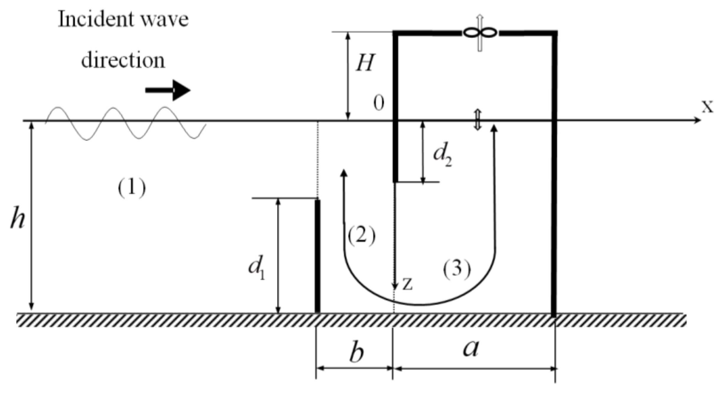
A new concept OWC device, modified from the conventional OWC system, was proposed by Boccotti [10]. It is called a U-shaped oscillating water column device, which adds a bottom-mounted vertical barrier in front of the existing OWC device. Consequently, wave energy is not transmitted directly into the internal fluid region of the air chamber, and the incident wave induces oscillatory motion of the U-shaped water column formed by the vertical barrier as shown in Figure 1. Conclusively, the air turbine is operated by the airflow in the chamber, which is caused by the internal surface displacement at one end of the U-shaped column. Investigations of hydrodynamic performance for a U-OWC device have been performed theoretically, numerically, and experimentally by many researchers since the concept was published. Boccotti [10] used the unsteady Bernoulli equation to establish the basis for a theoretical model of the oscillation of a U-shaped column. Later, Boccotti et al. [11] conducted a model experiment to verify the theoretical model. Malara and Arena [12] developed a hybrid numerical model applying the eigenfunction expansion method based on linear potential theory to the outer region of the U-OWC and the unsteady Bernoulli equation to the inner region. Malara et al. [13] derived the boundary integral equation based on the linear potential theory and developed a three-dimensional numerical model of the U-OWC device. Malara and Arena [14] proposed a semi-analytical approach for the estimation of hydrodynamic efficiency when multiple U-OWCs are arranged. It was found that an arrangement of several U-OWC devices reduces the hydrodynamic efficiency compared to independent U-OWC devices. Ning et al. [15] examined the effects of a vertical barrier on hydrodynamic performance using the higher-order boundary element method (HOBEM) based on the nonlinear potential theory including nonlinear free-surface boundary conditions.

An ANN model that is made up of multiple hidden layers allows the computational model to learn the correlation between features in the dataset [16]. ANN models are making crucial advances in solving problems that have held out against the artificial intelligence (AI) community for a long time. It has turned out to be outstanding at discovering complicated structures in high-dimensional data [17] and is therefore relevant to many fields of science, business, and government. Lawrence et al. [18] developed a hybrid neural network model for face recognition. Their system combines a local image sampling, a self-organizing map (SOM) neural network, and a convolutional neural network. Dahl et al. [19] proposed a novel context-dependent (CD) model for large-vocabulary speech recognition (LVSR) that leverages recent advances in the use of deep belief networks for phone recognition. They used a pre-trained deep neural network hidden Markov model (DNN-HMM) hybrid architecture that trains the DNN to produce a distribution over senones (tied triphone states) as its output. Rifaioglu et al. [20] reviewed deep learning-based identification of the interaction between drugs and their targets, something known as virtual screening. Recently, researchers have applied different machine learning techniques to optimize WECs systems. Sarkar et al. [21] used a machine learning algorithm to obtain the optimal layout of WECs in arrays. Deberneh [22] used wave data from nearshore floating buoys to train different machine learning regression models to predict the optimal site for nearshore wave energy harvesting. Masoumi [23] classified regions in the United States to improve decision-making in the design of wave-wind hybrid systems. They used an unsupervised K-means clustering algorithm based on wave height, wave period, and wind speed.

In the present study, the hydrodynamic performance of a 2D U-OWC is investigated in irregular waves using an analytical model. Then, an artificial neural network (ANN) model belonging to a supervised machine learning algorithm is used to obtain the optimal geometry of a U-OWC for maximizing power generation. As an analytical model, a MEEM based on linear potential theory is used to obtain hydrodynamic parameters (flow rates, air pressure, etc.). A sample set of input features comprising geometry of a vertical barrier and submergence depth of a chamber is created using the Latin hypercube sampling (LHS) method. Using the analytical model, output features such as conversion efficiency and wave force are calculated for given input features and wave conditions. Finally, a database including all the features is established for each energy period and a detailed feature study is conducted on the database to obtain correlations between the features. To search for the optimal geometric features for maximizing extracted power, an artificial neural network (ANN) model is chosen. After preprocessing the database, an ANN model is designed and trained to predict output features like conversion efficiency and wave forces in irregular waves. Using the well-trained ANN model, predictions are made for a very large sample set (4000 samples) and from these predictions, optimal design parameters of a U-OWC are determined.

This paper is organized as follows: Section 2 describes the analytical model of a 2D U-OWC device. In Section 3, the numerical calculation is performed using a developed analytical model. Section 4 designs an ANN model and predicts the conversion efficiency and wave force from irregular waves. Conclusions are presented in Section 5.

2. Analytical Model

A U-shaped OWC device installed at a constant water depth (h) is used as the analytical model. A U-OWC device is composed of an air chamber of length (a) and height (H) and a chamber wall that is submerged at $d_2$ below the water surface. The airflow in the chamber escapes through the turbine installed at the top. A bottom-mounted vertical barrier with a height of $d_1$ is placed apart at a distance of b from the chamber (see Figure 1). By adding a vertical barrier in front of the chamber, it looks like an oscillating U-tube, different from a conventional OWC. A two-dimensional Cartesian coordinate system is introduced, the origin is positioned at the location where the chamber wall and water surface meet, and the positive direction of the z-axis is set vertically downward. The energy of the incident wave going in the positive x-direction is partially reflected and some enters into the chamber and oscillates the water surface there. Electricity is produced by rotating the turbine installed on the top of the chamber.

It is assumed that the fluid is incompressible and inviscid, and the flow is irrotational so that linear potential theory can be used. The fluid particle velocity can then be described by the gradient of a velocity potential $\Phi (x,z,t)$. Assuming harmonic motion of frequency $\omega$, the velocity potential can be written as $\Phi (x,z,t)=\mathrm{Re}\left\{-\frac{igA}{\omega }\varphi (x,z)e^{-i\omega t}\right\}$, where A is the incident wave amplitude. Similarly, we can write down the wave elevation $\zeta (x,t)=\mathrm{Re}\left\{\eta (x)e^{-i\omega t}\right\}$ and oscillating air pressure $P_c(t)=\mathrm{Re}\left\{p_c{e}^{-i\omega t}\right\}$ in the chamber.

Under the assumption of linear potential theory, the velocity potential can be expressed as the sum of the scattering potential (${\varphi }_1$), i.e., the sum of incident potential (${\varphi }_0=e^{ik(x+b)}\frac{f_0(z)}{f_0(0)}$) and diffraction potential (${\varphi }_D$), and the radiation potential (${\varphi }_2$) due to oscillating air pressure in the chamber in the absence of an incident wave, as shown in Equation (1).

$$\varphi =-\frac{igA}{\omega }{\varphi }_1+p_c{\varphi }_2$$

(1)

The diffraction ${\varphi }_1$ and radiation ${\varphi }_2$ potentials satisfy the following boundary-value problem

$$\frac{{\partial }^2{\varphi }_j}{\partial x^2}+\frac{{\partial }^2{\varphi }_j}{\partial z^2}=0,\hspace{0.17em}\hspace{0.17em}\hspace{0.17em}\hspace{0.17em}j=1,2$$

(2)

with the following boundary conditions

$$\{\begin{array}{l}\frac{\partial {\varphi }_j}{\partial z}-\frac{{\omega }^2}{g}{\varphi }_j=0,\hspace{0.17em}\hspace{0.17em}\hspace{0.17em}\hspace{0.17em}\hspace{0.17em}\hspace{0.17em}\hspace{0.17em}\hspace{0.17em}\hspace{0.17em}\hspace{0.17em}\hspace{0.17em}\hspace{0.17em}\hspace{0.17em}\hspace{0.17em}\hspace{0.17em}x\le 0\\ \frac{\partial {\varphi }_j}{\partial z}-\frac{{\omega }^2}{g}{\varphi }_j=\frac{i\omega }{\rho g}{\delta }_{j2},\hspace{0.17em}\hspace{0.17em}\hspace{0.17em}\hspace{0.17em}\hspace{0.17em}\hspace{0.17em}0\le x\hspace{0.17em}\le a,\end{array}\hspace{0.17em}\hspace{0.17em}\mathrm{on}\hspace{0.17em}\hspace{0.17em}z=0$$

(3)

$$\frac{\partial {\varphi }_j}{\partial x}=0,\hspace{0.17em}\hspace{0.17em}\hspace{0.17em}\hspace{0.17em}\mathrm{on}\hspace{0.17em}\hspace{0.17em}\hspace{0.17em}\hspace{0.17em}\hspace{0.17em}\begin{array}{c}x=a\hspace{0.17em},\hspace{0.17em}\hspace{0.17em}0\le z\le h\\ x=0\hspace{0.17em},\hspace{0.17em}\hspace{0.17em}0\le z\le d_2\\ x=-b,\hspace{0.17em}c\le z\le h\end{array}\hspace{0.17em}$$

(4)

$$\frac{\partial {\varphi }_j}{\partial z}=0,\hspace{0.17em}\hspace{0.17em}\hspace{0.17em}\hspace{0.17em}\mathrm{on}\hspace{0.17em}\hspace{0.17em}\hspace{0.17em}z=h$$

(5)

$$\underset{x\to -\infty }{\lim }(\frac{\partial }{\partial x}+ik)\left(\begin{array}{l}{\varphi }_1-{\varphi }_0\\ {\varphi }_2\end{array}\right)=0.$$

(6)

where $c=h-d_1$, ${\delta }_{jk}$ is the Kronecker delta defined by ${\delta }_{jk}=1$ if $j=k$, and ${\delta }_{jk}=0$ if $j\ne k$.

2.1. Matched Eigenfunction Expansion Method

For applying a MEEM, the fluid domain is divided into three regions, as shown in Figure 1. Region (1) is defined by $x\le -b$, region (2) by $-b\le x\le 0$, and region (3) by $0\le x\le a$. By the method of separation of variables, the velocity potentials in each region can be written as:

$${\varphi }_j^{(1)}(x,z)=e^{-k_0(x+b)}\frac{f_0(z)}{f_0(0)}{\delta }_{j1}+{\displaystyle \sum _{n=0}^{\infty }{A}_{jn}^{}{e}^{k_n(x+b)}{f}_n(z)},$$

(7)

$${\varphi }_j^{(2)}(x,z)={\displaystyle \sum _{n=0}^{\infty }\left(B_{jn}^{}{e}^{k_n(x+b)}+C_{jn}^{}{e}^{-k_{n}x}\right)\hspace{0.17em}\hspace{0.17em}{f}_n(z)},$$

(8)

$${\varphi }_j^{(3)}(x,z)={\displaystyle \sum _{n=0}^{\infty }{D}_{jn}^{}\cosh k_n(x-a)f_n(z)}-\frac{i}{\rho \omega }{\delta }_{j2}$$

(9)

where $n=0$ represents the propagating mode, while each $n\ge 1$ corresponds to evanescent modes. The eigenvalues $(k_0=-ik,k_n,n=1,2,\dots )$ are the solutions of the dispersion equation given by $k_n\tan \hspace{0.17em}\hspace{0.17em}{k}_{n}h=-\frac{{\omega }^2}{g},\hspace{0.17em}\hspace{0.17em}n\ge 0$.

The vertical eigenfunctions $f_n(z),\hspace{0.17em}\hspace{0.17em}(n=0,1,2,..)$ are given by $f_n(z)=N_n^{-1}\cos \hspace{0.17em}{k}_n(z-h),$ with $N_n^2=\frac{1}{2}\left(1+\frac{\sin 2k_{n}h}{2k_{n}h}\right).$ The vertical eigenfunctions $f_n(z)$ form a complete orthogonal set in [0,h]:

$$\frac{1}{h}{\displaystyle {\int }_0^h{f}_n(z)f_m(z)}dz={\delta }_{mn}$$

(10)

where ${\delta }_{mn}$ is the Kronecker delta.

The unknown coefficients $A_{jn}^{},B_{jn}^{},C_{jn}^{},D_{jn}^{}$ in Equations (7)–(9) can then be determined by invoking the continuity of potential and horizontal velocity across $x=-b,0$.

$$\begin{array}{l}{\frac{\partial {\varphi }_j^{(1)}}{\partial x}|}_{x=-b}={\frac{\partial {\varphi }_j^{(2)}}{\partial x}|}_{x=-b}=\{\begin{array}{l}{U}_j^{(1)}(z),\hspace{0.17em}\hspace{0.17em}\hspace{0.17em}0\le z\le c\\ 0,\hspace{0.17em}\hspace{0.17em}\hspace{0.17em}\hspace{0.17em}\hspace{0.17em}\hspace{0.17em}\hspace{0.17em}\hspace{0.17em}\hspace{0.17em}\hspace{0.17em}\hspace{0.17em}c\le z\le h\end{array}\\ {\frac{\partial {\varphi }_j^{(2)}}{\partial x}|}_{x=0}={\frac{\partial {\varphi }_j^{(3)}}{\partial x}|}_{x=0}=\{\begin{array}{l}0,\hspace{0.17em}\hspace{0.17em}\hspace{0.17em}\hspace{0.17em}\hspace{0.17em}\hspace{0.17em}\hspace{0.17em}\hspace{0.17em}\hspace{0.17em}\hspace{0.17em}\hspace{0.17em}\hspace{0.17em}\hspace{0.17em}\hspace{0.17em}\hspace{0.17em}0\le z\le d_2\\ U_j^{(2)}(z),\hspace{0.17em}\hspace{0.17em}\hspace{0.17em}\hspace{0.17em}\hspace{0.17em}\hspace{0.17em}\hspace{0.17em}{d}_2\le z\le h\end{array}\end{array}$$

(11)

$$\begin{array}{l}{\varphi }_j^{(1)}(-b,z)={\varphi }_j^{(2)}(-b,z),\hspace{0.17em}\hspace{0.17em}\hspace{0.17em}\hspace{0.17em}0\le z\le c\\ {\varphi }_j^{(2)}(0,z)={\varphi }_j^{(3)}(0,z),\hspace{0.17em}\hspace{0.17em}\hspace{0.17em}\hspace{0.17em}\hspace{0.17em}\hspace{0.17em}\hspace{0.17em}\hspace{0.17em}\hspace{0.17em}\hspace{0.17em}{d}_2\le z\le h\end{array}$$

(12)

where $U_j^{(1)}(z),U_j^{(2)}(z)$ are the unknown horizontal fluid velocities at the openings.

After substituting Equations (7)–(9) into Equation (11), then multiplying both sides by $\{f_m(z):m=0,1,2,...\}$ and integrating over $[0,h]$, we obtain the following equations

$$\begin{array}{l}{A}_{jn}=\frac{1}{k_{n}h}{\displaystyle {\int }_0^c{U}_j^{(1)}(z)f_n(z)dz}+\frac{{\delta }_{n0}{\delta }_{j1}}{f_0(0)},\\ B_{jn}=\frac{1}{k_{n}h(1-e^{2k_{n}b})}\left({\displaystyle {\int }_0^c{U}_j^{(1)}(z)f_n(z)dz}-e^{k_{n}b}{\displaystyle {\int }_{d_2}^h{U}_j^{(2)}(z)f_n(z)dz}\right),\\ C_{jn}=\frac{1}{k_{n}h(1-e^{2k_{n}b})}\left(e^{k_{n}b}{\displaystyle {\int }_0^c{U}_j^{(1)}(z)f_n(z)dz}-{\displaystyle {\int }_{d_2}^h{U}_j^{(2)}(z)f_n(z)dz}\right),\\ D_{jn}=-\frac{1}{k_{n}h\sinh k_{n}a}{\displaystyle {\int }_{d_2}^h{U}_j^{(2)}(z)f_n(z)dz},\hspace{0.17em}\hspace{0.17em}\hspace{0.17em}\hspace{0.17em}n=0,1,2,\dots \end{array}$$

(13)

Using the above equations, four unknowns $A_{jn}^{},B_{jn}^{},C_{jn}^{},D_{jn}^{}$ can be expressed by two unknowns $U_j^{(1)}(z),U_j^{(2)}(z)$ and then applying the continuity of the velocity potential given by Equation (12), the following equations are readily derived

$$\begin{array}{l}{\displaystyle \sum _{n=0}^{\infty }\frac{f_n(z)}{k_{n}h}}\left(1+\frac{1}{\tanh k_{n}b}\right){\displaystyle {\int }_0^c{U}_j^{(1)}(z)f_n(z)dz}\\ -{\displaystyle \sum _{n=0}^{\infty }\frac{f_n(z)}{k_{n}h\sinh k_{n}b}}{\displaystyle {\int }_{d_2}^h{U}_j^{(2)}(z)f_n(z)dz}=-2\frac{f_0(z)}{f_0(0)}{\delta }_{j1}\end{array}$$

(14)

$$\begin{array}{l}-{\displaystyle \sum _{n=0}^{\infty }\frac{f_n(z)}{k_{n}h\sinh k_{n}b}}{\displaystyle {\int }_0^c{U}_j^{(1)}(z)f_n(z)dz}\\ +{\displaystyle \sum _{n=0}^{\infty }\frac{f_n(z)}{k_{n}h}}\left(\frac{1}{\tanh k_{n}a}+\frac{1}{\tanh k_{n}b}\right){\displaystyle {\int }_{d_2}^h{U}_j^{(2)}(z)f_n(z)dz}=-\frac{i}{\rho \omega }{\delta }_{j2}.\end{array}$$

(15)

Following Evans and Porter (1995), we can expand the horizontal fluid velocities $U_j^{(1)}(z)$ and $U_j^{(2)}(z)$ at the openings as a series of Chebyshev polynomials

$$\begin{array}{l}{U}_j^{(1)}(z)={\displaystyle \sum _{q=0}^{\infty }{a}_{jq}^{(1)}{u}_q^{(1)}(z)},\hspace{0.17em}\hspace{0.17em}\hspace{0.17em}\hspace{0.17em}\mathrm{on}\hspace{0.17em}\hspace{0.17em}\hspace{0.17em}0\le z\le c\\ U_j^{(2)}(z)={\displaystyle \sum _{q=0}^{\infty }{a}_{jq}^{(2)}{u}_q^{(2)}(z)},\hspace{0.17em}\hspace{0.17em}\hspace{0.17em}\hspace{0.17em}\mathrm{on}\hspace{0.17em}\hspace{0.17em}\hspace{0.17em}{d}_2\le z\le h\hspace{0.17em}\end{array}$$

(16)

where $a_{jq}^{(1)},a_{jq}^{(2)}(q=0,1,2,\dots )$ are the unknown expansion coefficients. $u_q^{(1)}(z),u_q^{(2)}(z)$, satisfying the free-surface boundary condition and the square-root singularity at the edge of the plate, are given by

$$\begin{array}{l}{\widehat{u}}_q^{(1)}(z)=u_q^{(1)}(z)-\frac{{\omega }^2}{g}{\displaystyle {\int }_z^c{u}_q^{(1)}(t)}dt\hspace{0.17em}=\frac{2{(-1)}^q}{\pi \sqrt{c^2-z^2}}{T}_{2q}\left(\frac{z}{c}\right),\\ u_q^{(2)}(z)=\frac{2{(-1)}^q}{\pi \sqrt{{(h-d_2)}^2-{(h-z)}^2}}{T}_{2q}\left(\frac{h-z}{h-d_2}\right),\end{array}$$

(17)

where $T_{2n}(x)=\frac{\sin [(2n+1)\theta ]}{\sin \theta },\hspace{0.17em}\hspace{0.17em}x=\cos \theta$ is the 2nd-order Chebyshev polynomial of the second kind.

Substituting Equation (16) into Equations (14) and (15), the coupled algebraic equations are obtained as follows:

$$\begin{array}{l}{\displaystyle \sum _{q=0}^{\infty }{a}_{jq}^{(1)}}{\displaystyle \sum _{n=0}^{\infty }\frac{F_{qn}^{(1)}{f}_n(z)}{k_{n}h}}\left(1+\frac{1}{\tanh k_{n}b}\right)-{\displaystyle \sum _{q=0}^{\infty }{a}_{jq}^{(2)}}{\displaystyle \sum _{n=0}^{\infty }\frac{F_{qn}^{(2)}{f}_n(z)}{k_{n}h\sinh k_{n}b}}=-2\frac{f_0(z)}{f_0(0)}{\delta }_{j1},\\ \\ -{\displaystyle \sum _{q=0}^{\infty }{a}_{jq}^{(1)}}{\displaystyle \sum _{n=0}^{\infty }\frac{F_{qn}^{(1)}{f}_n(z)}{k_{n}h\sinh k_{n}b}}+{\displaystyle \sum _{q=0}^{\infty }{a}_{jq}^{(2)}}{\displaystyle \sum _{n=0}^{\infty }\frac{F_{qn}^{(2)}{f}_n(z)}{k_{n}h}}\left(\frac{1}{\tanh k_{n}a}+\frac{1}{\tanh k_{n}b}\right)=-\frac{i}{\rho \omega }{\delta }_{j2},\end{array}$$

(18)

where

$$\begin{array}{l}{F}_{qn}^{(1)}=\{\begin{array}{l}{\displaystyle {\int }_0^c{u}_q^{(1)}(z)f_0(z)dz=\frac{{(-1)}^q\cosh kh{I}_{2q}(kc)}{N_0},\hspace{0.17em}\hspace{0.17em}n=0}\\ {\displaystyle {\int }_0^c{u}_q^{(1)}(z)f_n(z)dz=\frac{\cos k_{n}h{J}_{2q}(k_{n}c)}{N_n},\hspace{0.17em}\hspace{0.17em}\hspace{0.17em}\hspace{0.17em}\hspace{0.17em}\hspace{0.17em}\hspace{0.17em}\hspace{0.17em}\hspace{0.17em}\hspace{0.17em}\hspace{0.17em}\hspace{0.17em}n=1,2,..}\end{array}\\ F_{qn}^{(2)}=\{\begin{array}{l}{\displaystyle {\int }_{d_2}^h{u}_q^{(2)}(z)f_0(z)dz=\frac{{(-1)}^q{I}_{2q}(k(h-d_2))}{N_0},\hspace{0.17em}\hspace{0.17em}\hspace{0.17em}n=0}\\ {\displaystyle {\int }_{d_2}^h{u}_q^{(2)}(z)f_n(z)dz=\frac{J_{2q}(k_n(h-d_2))}{N_n},\hspace{0.17em}\hspace{0.17em}\hspace{0.17em}\hspace{0.17em}\hspace{0.17em}\hspace{0.17em}\hspace{0.17em}\hspace{0.17em}\hspace{0.17em}\hspace{0.17em}\hspace{0.17em}\hspace{0.17em}n=1,2,..}\end{array}\end{array}$$

By multiplying both sides of Equation (18) by $u_{q\prime }^{(1)}(z),u_{q\prime }^{(2)}(z),\hspace{0.17em}\hspace{0.17em}(q\prime =0,1,2,\dots )$, respectively, and integrating over $0\le z\le c$ and $d_2\le z\le h$, we can obtain the final algebraic equations by truncating n and q after N and M terms.

$${\displaystyle \sum _{q=0}^M{a}_{jq}^{(1)}}{\displaystyle \sum _{n=0}^N\frac{F_{qn}^{(1)}{F}_{q\prime n}^{(1)}}{k_{n}h}}\left(1+\frac{1}{\tanh k_{n}b}\right)-{\displaystyle \sum _{q=0}^M{a}_{jq}^{(2)}}{\displaystyle \sum _{n=0}^N\frac{F_{qn}^{(2)}{F}_{q\prime n}^{(1)}}{k_{n}h\sinh k_{n}b}}=-\frac{2F_{q\prime 0}^{(1)}}{f_0(0)}{\delta }_{j1},$$

(19)

$$\begin{array}{l}-{\displaystyle \sum _{q=0}^M{a}_{jq}^{(1)}}{\displaystyle \sum _{n=0}^N\frac{F_{qn}^{(1)}{F}_{q\prime n}^{(2)}}{k_{n}h\sinh k_{n}b}}+{\displaystyle \sum _{q=0}^M{a}_{jq}^{(2)}}{\displaystyle \sum _{n=0}^N\frac{F_{qn}^{(2)}{F}_{q\prime n}^{(2)}}{k_{n}h}}\left(\frac{1}{\tanh k_{n}a}+\frac{1}{\tanh k_{n}b}\right)\\ =-\frac{i}{\rho \omega }{\delta }_{j2}{\displaystyle {\int }_{d_2}^h{u}_{q\prime }^{(2)}(z)dz}=-\frac{i}{\rho \omega }{\delta }_{j2}{\delta }_{q^{\prime }0}\end{array}$$

(20)

By solving the coupled algebraic Equations (19) and (20), the unknown expansion coefficients $a_{jq}^{(1)},a_{jq}^{(2)}(j=1,2;q=0,1,2,\dots ,M)$ can be readily determined. Subsequently, the unknowns $A_{jn}^{},B_{jn}^{},C_{jn}^{},D_{jn}^{}(j=1,2;n=0,1,2,\dots ,N)$ in each region can be obtained from Equations (13) and (16).

2.2. Flux at the Internal Surface

The flux ($Q(t)=\mathrm{Re}\left\{q{e}^{-i\omega t}\right\}$) at the internal surface can be obtained by integrating the scattered and radiated potentials over the internal surface.

$$\begin{array}{l}q=-{\displaystyle {\int }_0^a\frac{\partial \varphi }{\partial z}}dx=A{q}_1+p_c{q}_2,\\ q_1=\frac{ig}{\omega }{\displaystyle {\int }_0^a{\frac{\partial {\varphi }_1^{(3)}}{\partial z}|}_{z=0}}dx,\\ q_2=-{\displaystyle {\int }_0^a{\frac{\partial {\varphi }_2^{(3)}}{\partial z}|}_{z=0}}dx=-(B-iC),\end{array}$$

(21)

where $q_1$ is the flux at the internal surface due to incident wave, and $q_2$ due to the oscillating pressure inside the chamber. $C$ is in phase with the flux acceleration and has a similar characteristic of the added mass (i.e., radiation admittance). $B$ is in phase with the flux velocity having an attribute of radiation damping (i.e., radiation conductance).

The horizontal wave forces $F_i=\mathrm{Re}\left\{f_i\hspace{0.17em}{e}^{-i\omega t}\right\}\hspace{0.17em}(i=1,2)$ on the vertical barrier and chamber wall can be found by integrating pressure differences.

$$\begin{array}{l}{f}_1=\rho gA{\displaystyle {\int }_c^h\left[{\varphi }_1^{(1)}(-b,z)-{\varphi }_1^{(2)}(-b,z)\right]dz},\\ f_2=\rho gA{\displaystyle {\int }_0^{d_2}\left[{\varphi }_1^{(2)}(0,z)-{\varphi }_1^{(3)}(0,z)\right]dz},\end{array}$$

(22)

The reflection coefficient of a U-OWC is written by

$$R_f=\left(A_{10}+\frac{i\omega }{g}{p}_c{A}_{20}\right)f_0(0).$$

(23)

2.3. Oscillating Air Pressure

To determine the oscillating air pressure $P_c=\mathrm{Re}\left\{p_c\hspace{0.17em}{e}^{-i\omega t}\right\}$ in the chamber, a continuity equation is used, for which the rate of change of mass inside the chamber is equal to the mass flux through the turbine. It is assumed that the air in the chamber is a compressible fluid, and the compression and expansion follow an adiabatic process.

$${\rho }_a\frac{d{V}_c}{dt}+\frac{{\rho }_a{V}_o}{\gamma P_{atm}}\frac{d{P}_c}{dt}=-{\rho }_a{Q}_t.$$

(24)

where ${\rho }_a$ is the air density; $\gamma (=1.4)$ the specific heat for an adiabatic situation; $P_{atm}$ atmospheric pressure and; $V_o(=aH)$ the volume of the air chamber. The flux $Q_t(=C_t{P}_c)$ through the turbine is assumed to be proportional to the air chamber pressure. $C_t(=\widehat{K}D/{\rho }_a\widehat{N})$ is the function of the damping coefficient ($\widehat{K}$) that is dependent on the shape of a turbine, turbine diameter ($D$), and rotational velocity ($\widehat{N}$) of a turbine.

In Equation (24), $\frac{d{V}_c}{dt}$ is the linearized rate of total upward displacement of the water surface inside the chamber and is equal to the upward flux $-Q(t)$ at the internal surface. For simple harmonic motion, $\frac{d{V}_c}{dt}$ can be written by

$$\frac{d{V}_c}{dt}=-Q(t)=-\mathrm{Re}\left\{(A{q}_1+p_c{q}_2)e^{-i\omega t}\right\}.$$

(25)

When combining Equation (25) with Equation (24), we obtain the chamber pressure

$$p_c=\frac{A{q}_D}{C_t+B-i\left(\frac{\omega V_o}{\gamma P_{atm}}+C\right)}.$$

(26)

2.4. Extracted Power

The power output is the time-averaged rate of work done by the chamber pressure pushing air through the turbine.

$$\overline{P}=\frac{1}{2}{C}_t{\left|p_c\right|}^2=\frac{1}{2}\frac{C_t{\left|A{q}_D\right|}^2}{{(C_t+B)}^2+{(\frac{\omega V_o}{\gamma P_{atm}}+C)}^2}.$$

(27)

Thus, the conversion efficiency can be calculated by dividing the incident wave power ${\overline{P}}_w=\frac{1}{2}\rho g{A}^2{C}_g$ per unit width of a regular wave with amplitude A.

$$E_{ff}=\frac{\overline{P}}{P_w}=\frac{C_t}{\rho g{C}_g}{\left|\frac{p_c}{A}\right|}^2.$$

(28)

where $C_g$ is the group velocity.

There is an optimal turbine constant that maximizes the conversion efficiency at each wave frequency. The optimal turbine constant, ${(C_t)}_{opt}$, can be obtained by imposing $d{E}_{ff}/d{C}_t=0$, which yields

$${\left(C_t\right)}_{opt}=\sqrt{B^2+{(\frac{\omega V_o}{\gamma P_{atm}}+C)}^2}$$

(29)

2.5. Extracted Power in Irregular Waves

The variance of the oscillating chamber pressure in irregular waves can be written by using Equation (26).

$${\sigma }_p^2={{\displaystyle {\int }_0^{\infty }\left|\frac{p_c}{A}(\omega )\right|}}^2\cdot S_{\eta \eta }(\omega )d\omega$$

(30)

where $S_{\eta \eta }$ is the incident wave spectrum. In the present study, a Pierson–Moskowitz (PM) spectrum is used

$$S_{\eta \eta }(\omega )=262.99\frac{H_{1/3}^2}{T_E^4{\omega }^5}\exp \left(-\frac{1051.97}{T_E^4{\omega }^4}\right)$$

(31)

where $H_{1/3}(=4\sqrt{m_0})$ is the significant wave height and $T_E(=2\pi \frac{m_{-1}}{m_0})$ the energy period and $m_n(={\displaystyle {\int }_0^{\infty }{S}_{\eta \eta }(\omega ){\omega }^{n}d\omega })$ the n-th order moment of the area under the spectral curve.

When the irregular wave is incident to the OWC, the maximum power per unit width is given by

$${\overline{P}}_{irr}={\left(C_t\right)}_{opt}{\sigma }_p^2,\hspace{0.17em}$$

(32)

As the optimal turbine constant ${(C_t)}_{opt}$ is a function of wave frequency, in irregular waves, we use the ${(C_t)}_{opt}$ value at the particular wave frequency that may be equal to the resonance frequency of piston-mode or energy frequency.

The maximum conversion efficiency of OWC attainable in irregular waves is

$${\eta }_{irr}=\frac{{\overline{P}}_{irr}}{{\overline{P}}_{w,irr}}.$$

(33)

where the denominator ${\overline{P}}_{w,irr}$ in Equation (33) is the irregular wave power per unit width and given by

$${\overline{P}}_{w,irr}=\rho g{\displaystyle {\int }_0^{\infty }{S}_{\eta \eta }(\omega )C_g(\omega )d\omega \approx \frac{1}{64\pi }}\rho g^2{H}_{1/3}^2{T}_E$$

(34)

Both the wave force spectrums on the vertical barrier (i = 1) and chamber wall (i = 2) in irregular waves are defined as

$$S_f^{(i)}(\omega )={\left|\frac{f_i(\omega )}{A}\right|}^2\cdot S_{\eta \eta }(\omega ),\hspace{0.17em}\hspace{0.17em}i=1,2$$

(35)

The significant wave forces can be obtained from integrating the above spectrums

$${\left(f_i\right)}_{1/3}=4\sqrt{{\displaystyle {\int }_0^{\infty }{S}_f^{(i)}(\omega )d\omega }},\hspace{0.17em}\hspace{0.17em}i=1,2$$

(36)

3. Numerical Calculation

3.1. Validation Test

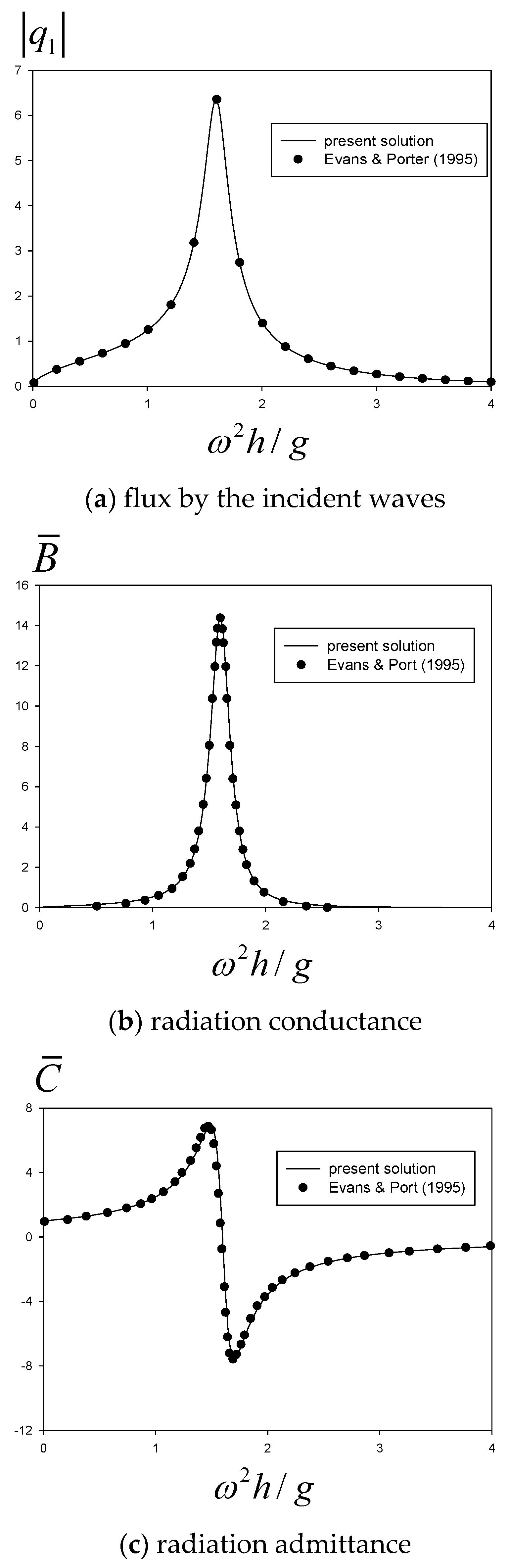
For verifying the validity of the present MEEM solutions, the calculation results are compared with those of Evans and Porter (1995) in Figure 2. The comparison model is a typical two-dimensional rectangular OWC device with no vertical barrier ($d_1=0$). The non-dimensional chamber length ($a/h$) and submerged depth ($d_2/h$) are 1/8 and 0.5, respectively. The x-axis is the dimensionless frequency (${\omega }^{2}h/g$), and the y-axis denotes the fluxes ($q_1,q_2(=-B+iC)$) at the internal surface due to the incident wave and oscillating chamber pressure. The radiation conductance ($B$) and radiation admittance ($C$) are non-dimensionalized by $\overline{B}=\frac{\rho g}{\omega a}B$ and $\overline{C}=\frac{\rho g}{\omega a}C$. The number of eigenfunctions of the z-axis used in the calculation is $N=100$, and the number of Galerkin expansion series is $M=10$. The analytical solutions are in exact agreement with the results of Evans and Porter (1995). From the comparison, $N=100$ and $M=10$ are equally used in the following calculations.

3.2. Design Features

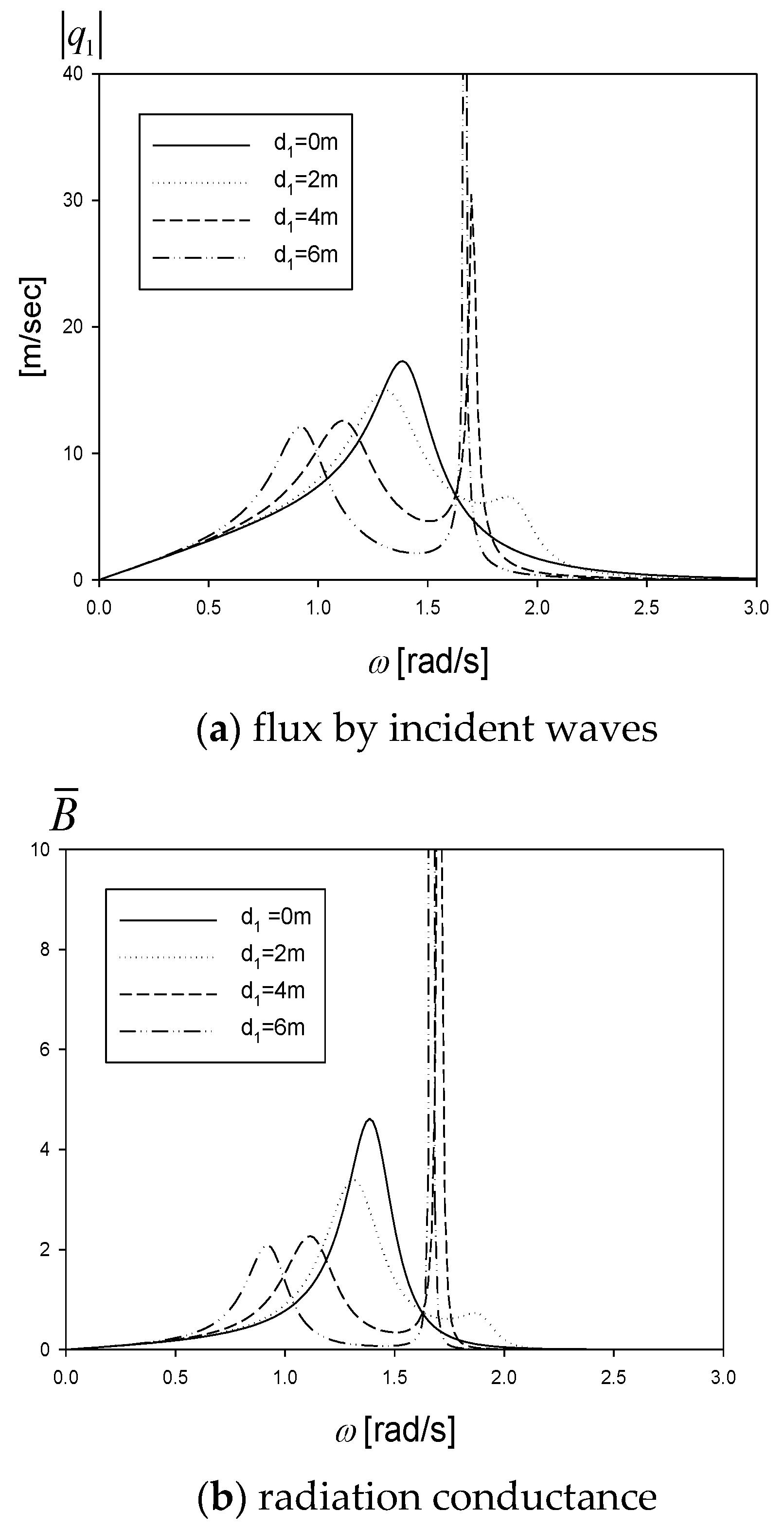
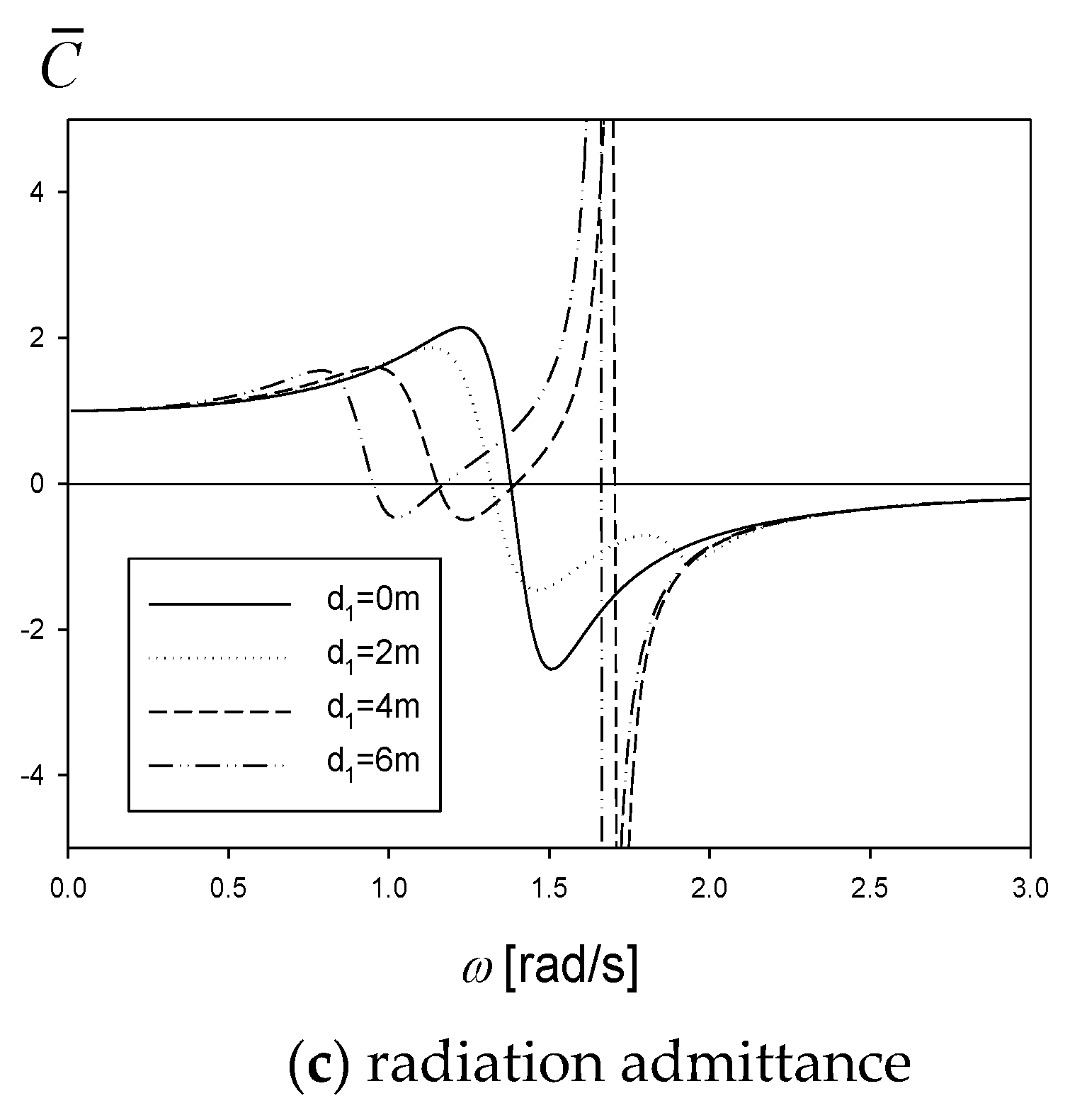
Figure 3a shows the flux at the internal surface by the incident wave as a function of the barrier height ($d_1$$=0,\hspace{0.17em}\hspace{0.17em}2,\hspace{0.17em}4,\hspace{0.17em}\hspace{0.17em}6\hspace{0.17em}\mathrm{m}$) and wave frequency. The chamber length (a) and submerged depth ($d_2$) are 3 m equally, the barrier distance (b) 1.5 m, and the water depth (h) 10 m. Two resonance peaks are shown within the entire wave frequency range ($0<\omega <3\hspace{0.17em}\mathrm{rad}/\mathrm{s}$). The first resonance, which seems a little wider and belongs to the lower-frequency region, occurs in the chamber region (3). It is called the piston-mode resonance, where the water surface goes up and down in unison at resonance, being different from the sloshing-mode resonance. The second spike-like peak attributes to the piston-mode resonance in the fluid region (2) existing between the vertical barrier and chamber wall. In particular, the second resonance is more conspicuous in the enclosed fluid region, which can be made by increasing the barrier height, and disappears when $d_1=0$, as expected. As the barrier height increases, the first resonance frequency decreases to 1.34, 1.26, 1.10, and 0.94 rad/s, and its peak value and width are also reduced. In Figure 3b,c, the flux by the oscillating air pressure is investigated under the same conditions as in Figure 3a. The non-dimensional radiation admittance ($\overline{C}$) increases with the wave frequency and changes abruptly from a positive to a negative value at the particular frequencies which coincide with the piston-mode resonance frequencies of each region. On the other hand, the non-dimensional radiation conductance ($\overline{B}$) has a maximum value at the same frequencies. This unique phenomenon occurs when a fluid region inducing resonance is present inside the oscillating system. As the barrier height increases, both the peak value and peak frequency at the first resonance decrease.

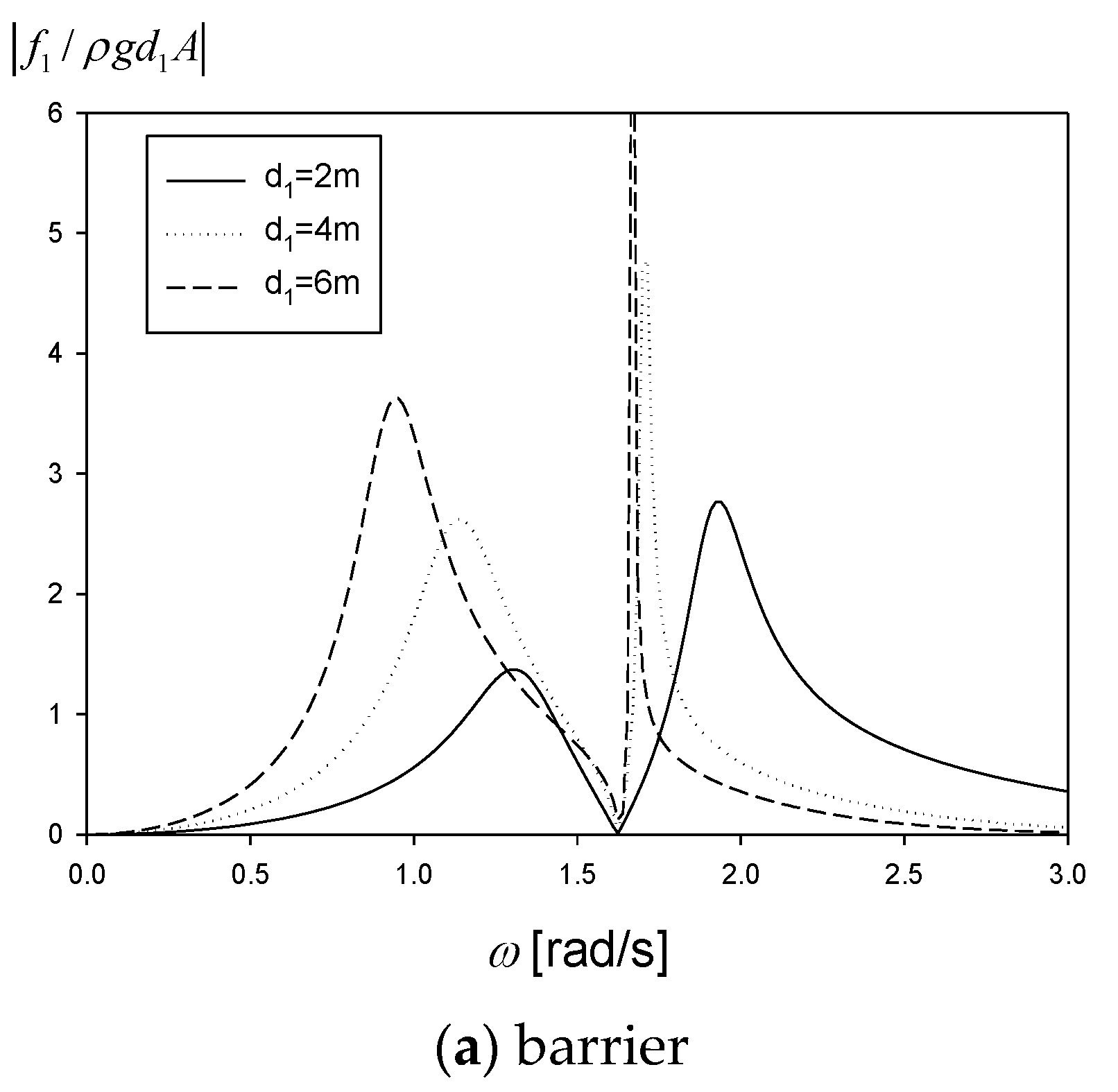
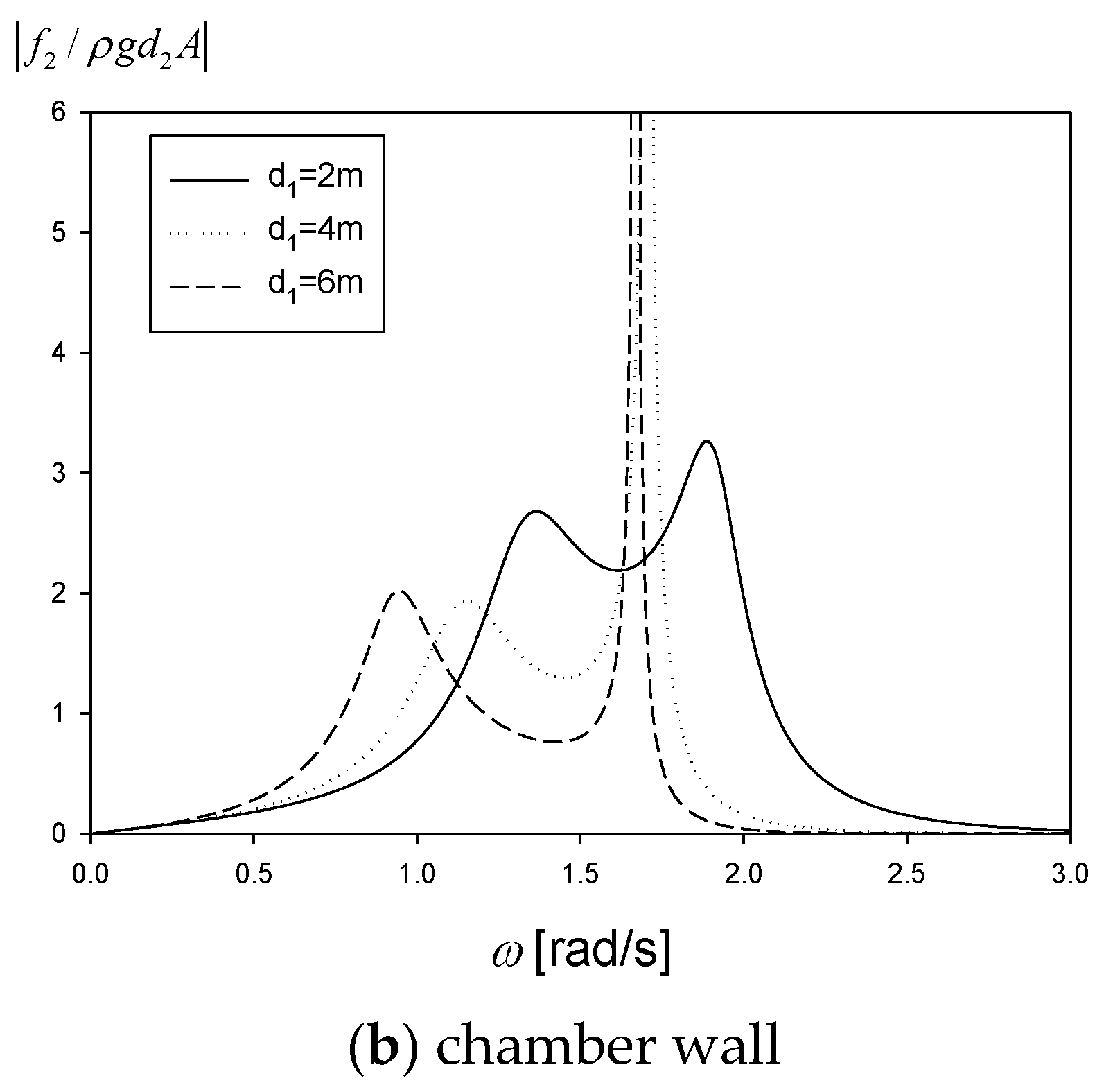
Figure 4 shows the non-dimensional wave forces on the barrier and chamber wall when the barrier height $d_1$ increases to 2, 4, and 6 m. As the barrier height increases, the wave force on the barrier increases, while the wave force on the chamber wall decreases by the effect of wave blocking by the barrier. The maximum wave forces occur at each resonance frequency. With an increase of the barrier height, the first resonant wave force on the barrier moves to the low-frequency region and increases, whereas the second resonant wave force shows the sharp reduction of resonant width.

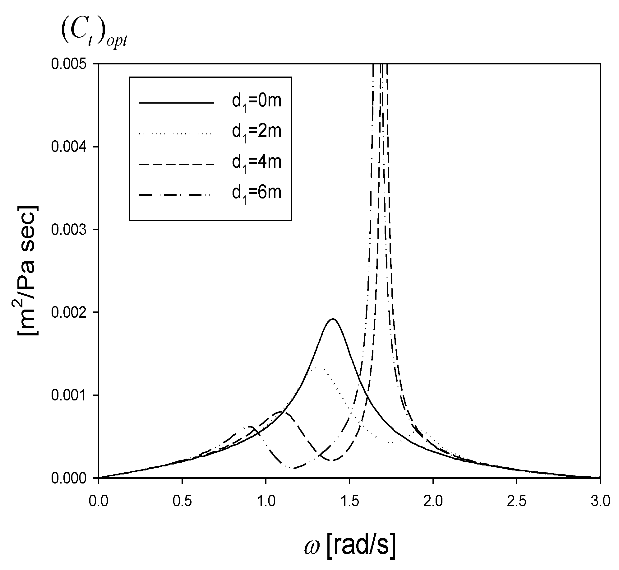
Figure 5 plots the optimum turbine constant (${(C_t)}_{opt}$) given in Equation (29) according to the barrier height. The optimum turbine constant is a kind of PTO (Power Take-off) damping constant that inevitably appears when converting wave energy into mechanical energy. As seen in Figure 5, the optimum turbine constant is a function of wave frequency and has a maximum value at each resonance frequency. Based on this, we can select the optimum turbine constant responding to the frequency of the incoming waves.

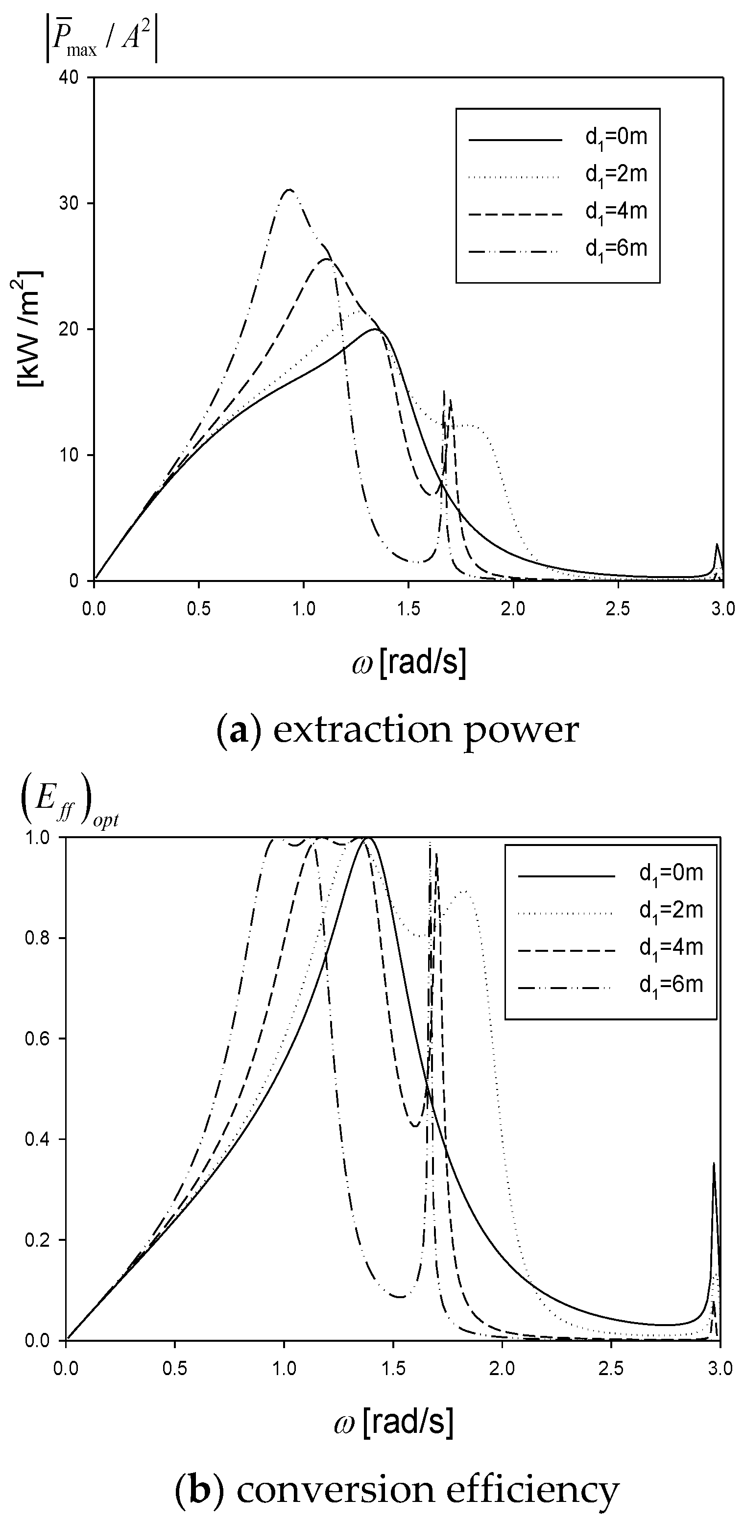
Figure 6 shows the extracted power and conversion efficiency when the optimum turbine constant given in Figure 5 is applied. As expected, it can be seen that the extracted power and conversion efficiency gives peak values at each resonance frequency. In particular, the first resonance that occurs in the chamber significantly affects the power extraction compared with the second spike-like resonance. However, though the second resonance may be insignificant, it helps expand the range of the wave frequency of good performance, and consequently plays an important role in absorbing wave energy from irregular waves. In addition, power extraction and conversion efficiency are both sensitive to barrier height. Furthermore, if adjusting the barrier height mechanically, we can enhance the power extraction. In Figure 6, the U-shaped OWC with the added proper vertical barrier has a positive effect on the wave energy production, especially at the low-frequency region and is, as a whole, superior to the conventional OWC without a barrier. This conclusion is, however, based on potential theory and does not consider minor power loss by viscous-flow separation when passing through the front barrier.

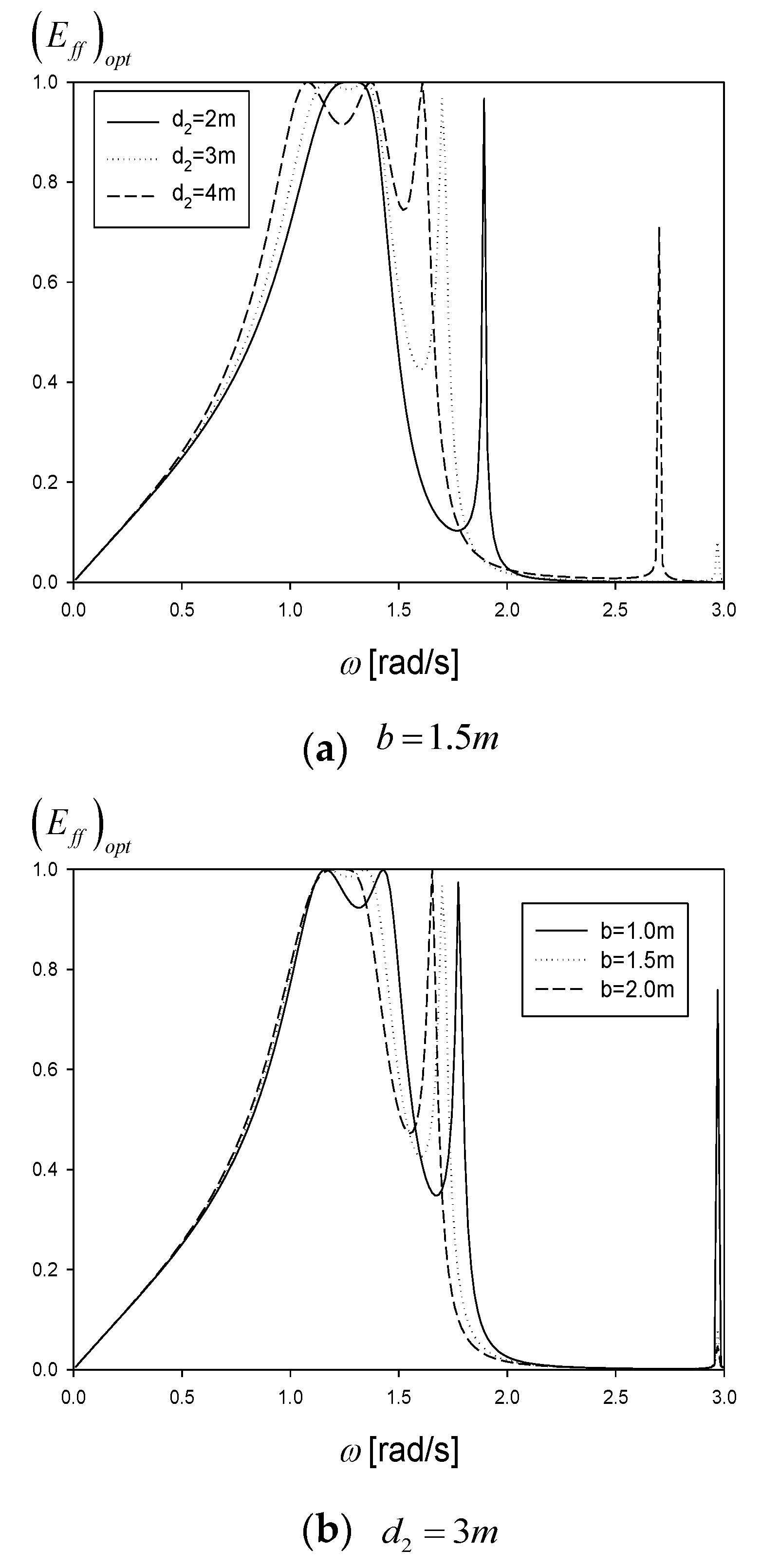
In Figure 7, the conversion efficiency is plotted with the change of the barrier distance (b). The barrier distance has more influence on the spike-like resonance frequency by changing the size of the fluid region (2). It can be seen that the second resonance frequency moves to the low-frequency region as the barrier distance increases. However, the first resonance does not show significant change except a slight decrease in the resonance width. This means that the barrier height is a more important design parameter than the barrier distance in the power extraction of a U-OWC.

3.3. Efficiency in Irregular Waves

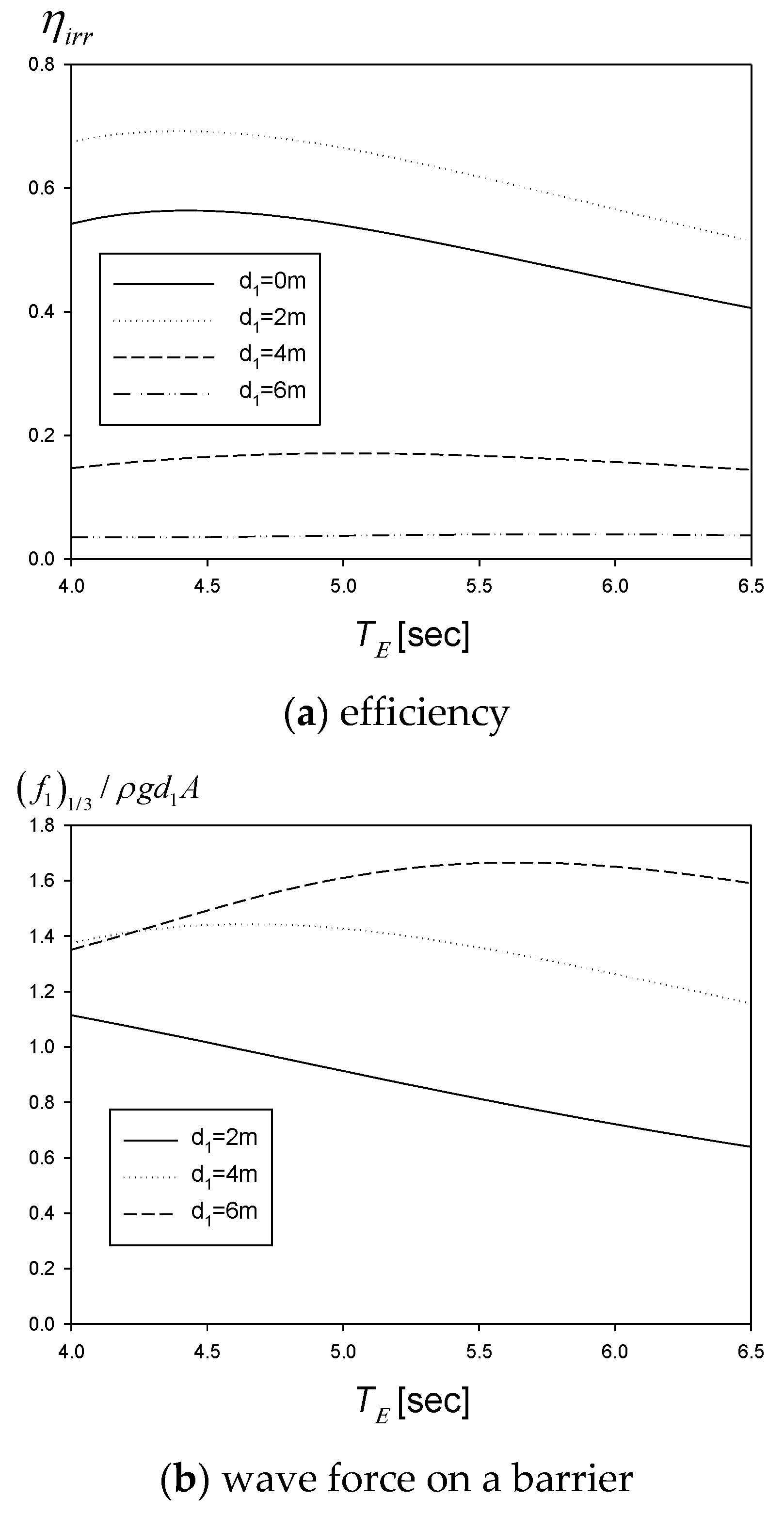
Next, let us consider the power production and conversion efficiency of a U-OWC device in irregular waves. As seen in Equation (32), we need the optimal turbine constant, which is a function of wave frequency. It is impossible to change the turbine constant instantaneously in irregular waves with wave frequencies changing from moment to moment. Therefore, we have to choose an appropriate representative value of the optimum turbine constant. In the present study, the ${(C_t)}_{opt}$ value at the first resonance frequency is chosen as the representative value in irregular waves. The wave spectrum used in the calculation is a PM (Pierson–Moskowitz) spectrum with a significant wave height $H_{1/3}$ of 1.0 m. Figure 8a shows the conversion efficiency as a function of the energy period and barrier height. The other variables are fixed at $h=10 \mathrm{m},a=3 \mathrm{m},d_2=3 \mathrm{m},b=1.5 \mathrm{m}$. Corresponding to the barrier height, the first resonance period in the chamber region is 4.69, 4.98, 5.71, and 6.68 s with the barrier heights d₁ = 0, 2, 4, and 6 m. It is seen that the U-OWC gives the maximum conversion efficiency of 0.70 at T_E = 4.5 s and d₁ = 2.0 m, which shows an improved efficiency over the conventional OWC with no-barrier which had a maximum conversion efficiency of 0.56. The further increase of the barrier height reduces the conversion efficiency regardless of the energy period. This means that there exists an optimal value of the barrier height.

The non-dimensional significant wave force on the barrier is shown in Figure 8b as a function of the barrier height and energy period. The higher the barrier height, the larger the wave forces on the barrier especially at longer waves. Considering the above results, we have to design the optimal barrier height with a strategy that gives the higher conversion efficiency and lower wave force.

4. Design Optimization Using an ANN Model

For obtaining optimal design parameters of the U-OWC in irregular waves, we adopt a supervised ANN model. The creation of the database, feature study, ANN model description, and training and validation of the model are explained in this section.

4.1. Database

Using the analytical model described in Section 2, the database is created from the following input features; barrier height $(d_1)$, submergence depth of a chamber wall $(d_2)$, and barrier distance (b), and the following output features; conversion efficiency $\left({\eta }_{irr}\right)$ and non-dimensional significant wave force $\left({\left(f_1\right)}_{1/3}/\rho g{d}_{1}A\right)$ on the barrier. All other parameters are taken as fixed values: water depth ($h=10 \mathrm{m}$), chamber length (a = 5 m), and significant wave height ( $H_{1/3}=1 \mathrm{m}$). Three databases are made for three different energy periods $\left(T_E=4\hspace{0.17em},5\hspace{0.17em},6\hspace{0.17em}\hspace{0.17em}\mathrm{s}\right)$.

The sampling method is of great importance in the ANN model. A good sampling method can result in a more reasonable sample distribution, leading to a better neural network model with higher accuracy. In the present study, Latin hypercube sampling (LHS) [24] is utilized to generate random sample points. The sample space of three input features is taken as follows:

$$\{\begin{array}{l}{d}_1\in \left[0,6.66\right]\\ d_2\in \left[1,6\right]\\ b\hspace{0.17em}\hspace{0.17em}\in \left[0.1,5\right]\end{array}$$

(37)

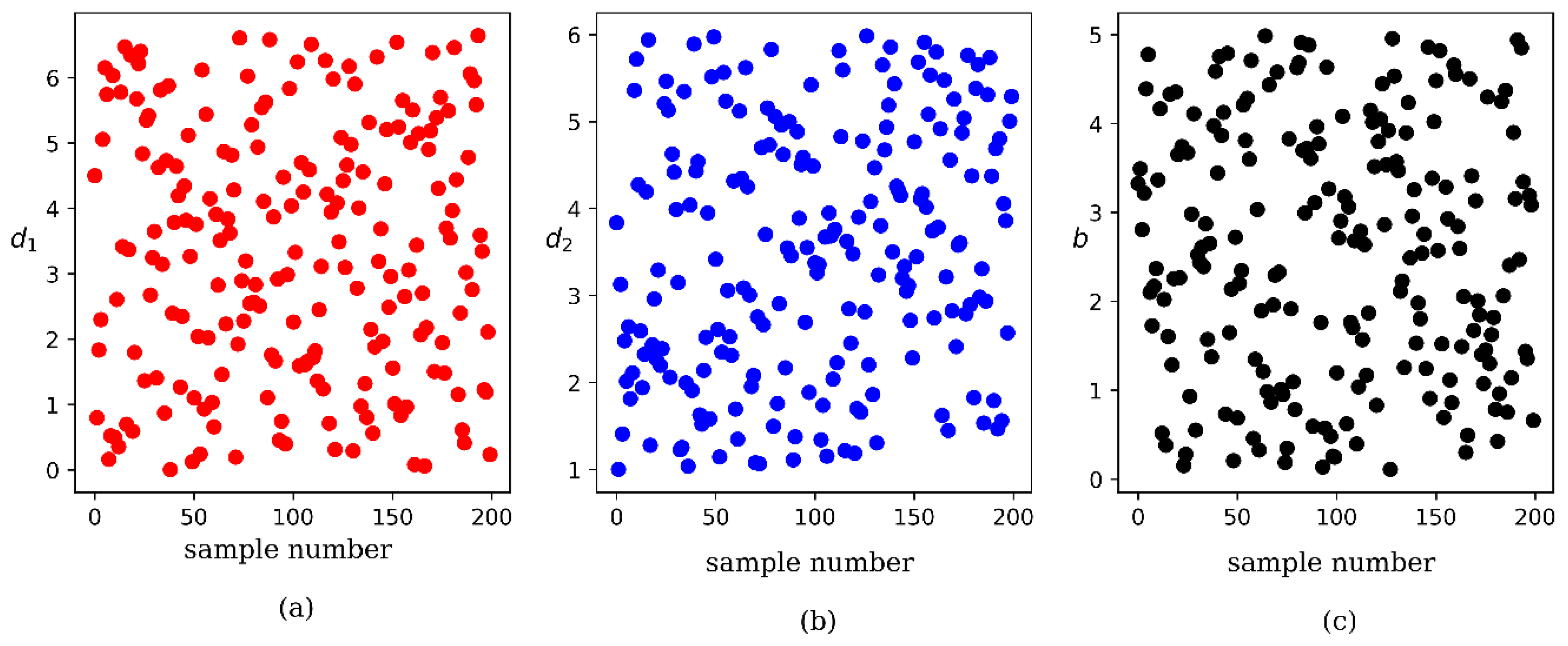
Using the LHS, we can fill the sample space within its bounds by maximizing the stratification of each edge distribution, which improves uniformity. A sample set containing 200 samples was established and scatter diagrams of the samples are displayed in Figure 9. Each input feature fills the whole sample space and the standard deviation seems to be small as shown in Figure 9.

4.2. Characteristics of Features

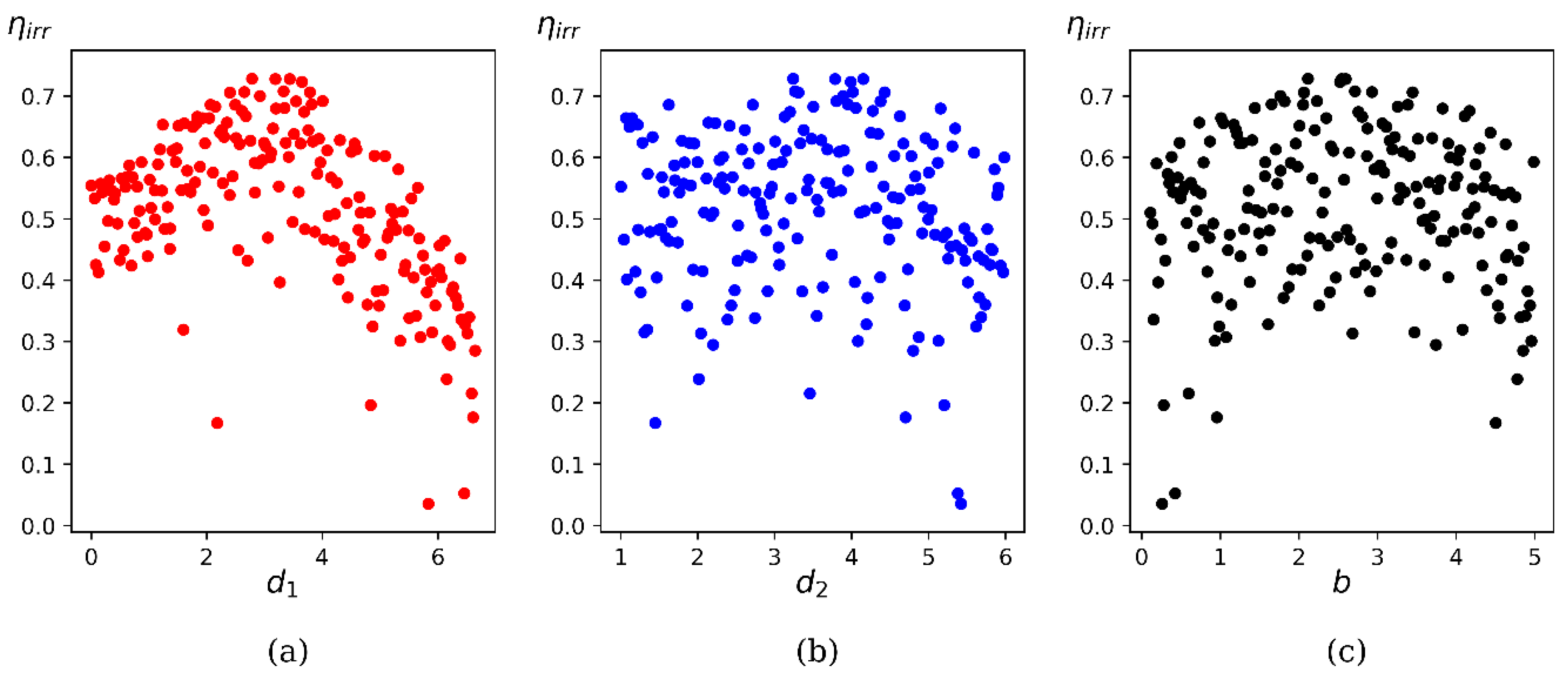
A feature study is conducted on the database to obtain the correlation between the input and output features. Figure 10 and Figure 11 show the scatter plots of the conversion efficiency (${\eta }_{irr}$) and non-dimensional significant wave force (${\left(f_1\right)}_{1/3}/\rho g{d}_{1}A$) on the barrier at fixed energy period $T_E=5 \mathrm{s}$ in irregular waves. Variation of each output feature versus three input features is displayed in the separate figure. There exists a significant correlation between the conversion efficiency and barrier height as shown in Figure 10a and the correlation coefficient is 0.467 at $T_E=5 \mathrm{s}$. The correlation between the conversion efficiency and other input features ($d_2$,b) is observed to be less significant when compared to $d_1$.

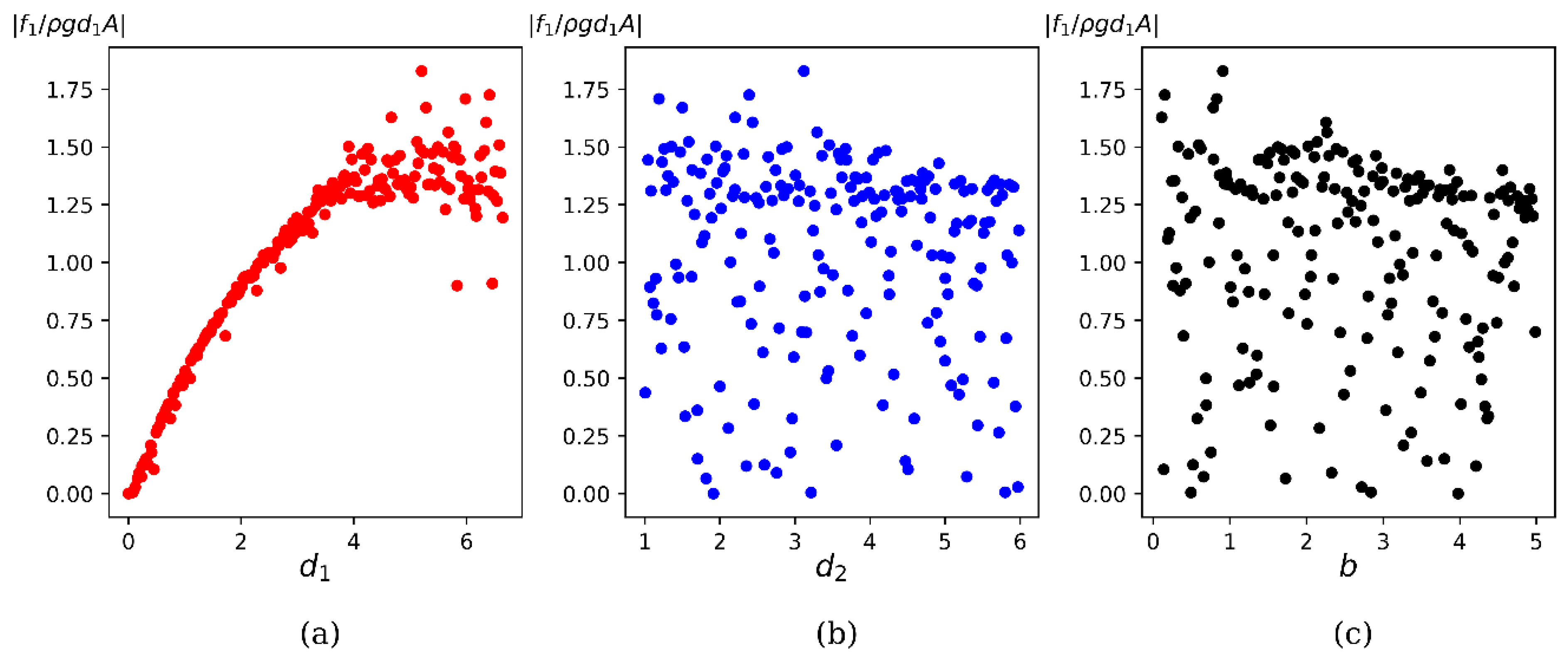
Variation of non-dimensional significant wave force (${\left(f_1\right)}_{1/3}/\rho g{d}_{1}A$) on the barrier as a function of the input features is shown in Figure 11. It is observed that a strong correlation occurs between the wave force and barrier height ($d_1$). The correlation coefficient is 0.884. The wave forces increase steadily with the barrier height as expected. As in the previous figure, the correlation of ${\left(f_1\right)}_{1/3}/\rho g{d}_{1}A$ with other input features (d₂,b) is insignificant.

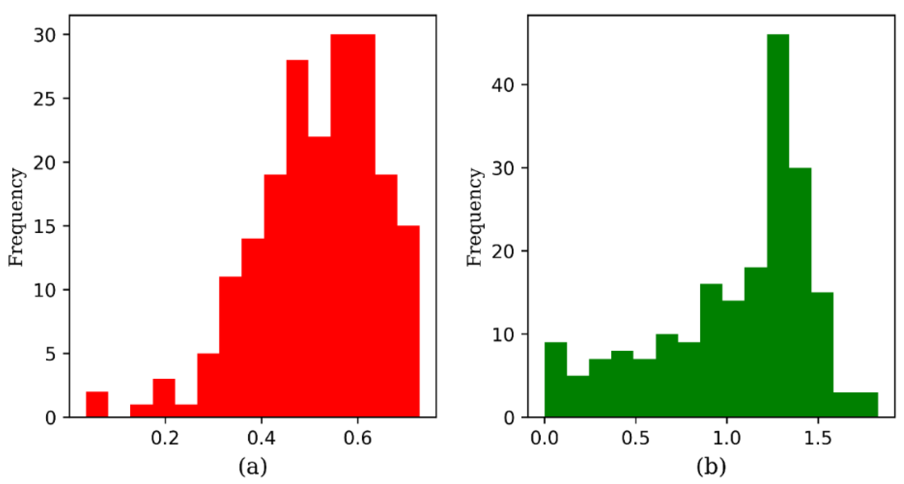
Figure 12 shows the distribution of the output features (${\eta }_{irr}$, ${\left(f_1\right)}_{1/3}/\rho g{d}_{1}A$). Both the output features are randomly distributed on the sample space but show a high probability of occurrence in the specific range of ${\eta }_{irr}\in [0.5,0.7]$ and ${\left(f_1\right)}_{1/3}/\rho g{d}_{1}A\in [1.2,1.4]$

4.3. Preprocessing of the Data

The whole data is split into the training and test data. The training data are used to train the ANN model, while the test data are reserved to evaluate the trained ANN model. Approximately 70 percent of the 200 data is allotted to the training data and the remaining 30 percent is assigned to test data. All data are allocated randomly.

The input features in the present database have inherent numerical values that are different from each other, which may affect the performance of the ANN model. So, the input features are scaled to a standard range using the standard scaler $\frac{x-\overline{x}}{\sigma (x)}$, where $\overline{x}$ means a mean value and $\sigma (x)$ standard deviation.

4.4. Description of an ANN Model

An ANN regression model based on a feedforward neural network is used to predict the optimal design features of the U-OWC. The advantage of an ANN model lies in the fact that it is capable of learning the strong nonlinear relationship between the input and output features. Before training the ANN model, we need to optimize the hyperparameters [25] of the model: the number of hidden layers, learning rate, batch size, and regularization parameter. To obtain these optimal hyperparameters, an exhaustive search algorithm is used with the ANN regression model. The best hyperparameters for each energy period are listed in

Table 1. Optimal hyperparameters of an ANN model.

Hyperparameter	${\mathit{T}}_{\mathit{E}}=\mathbf{4} \mathbf{s}$	${\mathit{T}}_{\mathit{E}}=\mathbf{5} \mathbf{s}$	${\mathit{T}}_{\mathit{E}}=\mathbf{6} \mathbf{s}$
hidden layer	(30,30)	(30, 30, 30)	(20, 20, 20)
learning rate	0.001	0.001	0.005
batch size	20	50	100
regularization parameter	0.1	0.01	0.01

.

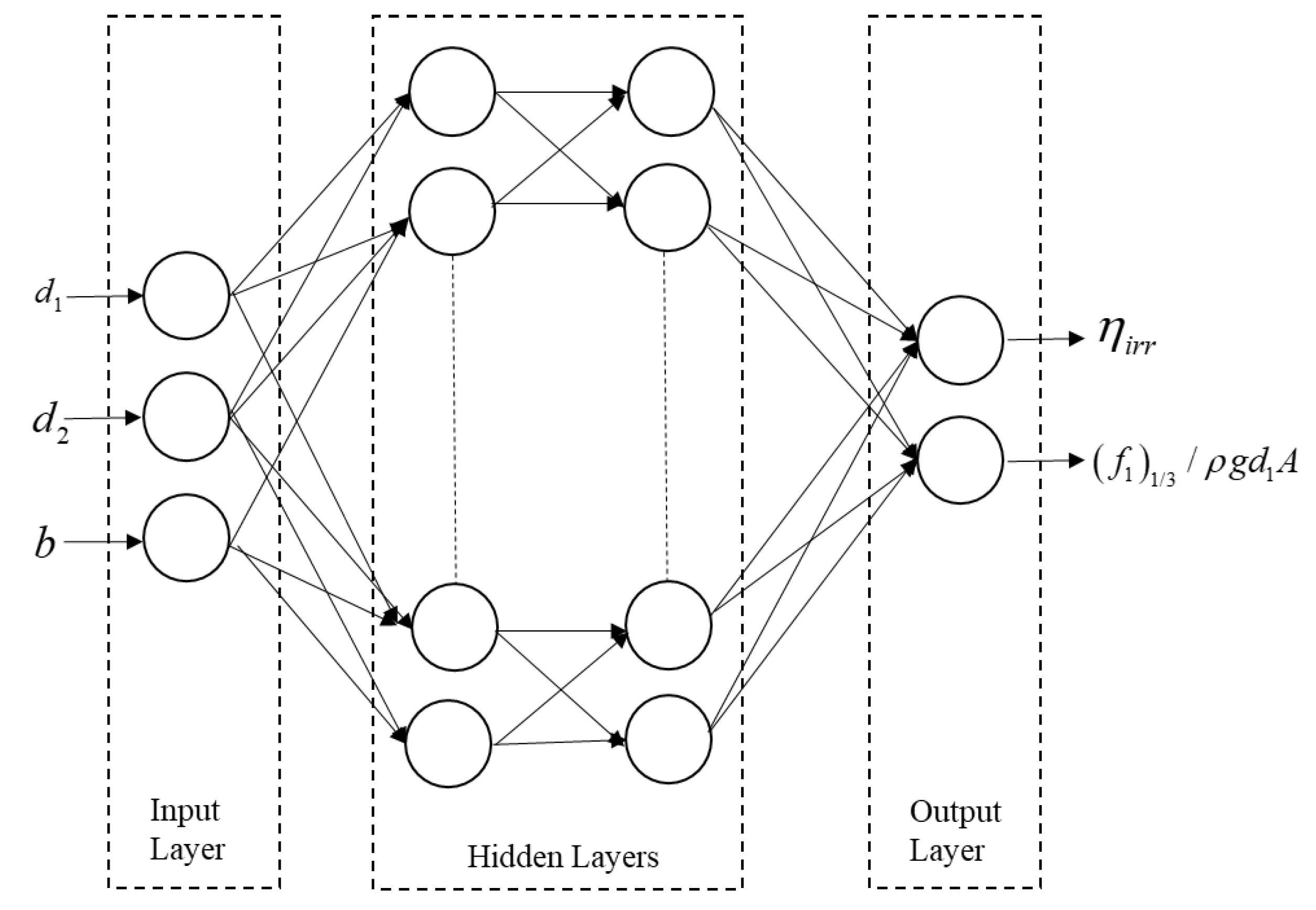
The general architecture of the present ANN model with hidden layers is shown in Figure 13. The leftmost input layer consists of neurons representing three input features. Each neuron in the hidden layer transforms the data from the previous layer with a weighted linear summation followed by a nonlinear activation function. For a single neuron with $m$ input features, the linear summation can be written as,

$$h\left(x\right)=\tilde{b}+{\displaystyle \sum _{i=1}^m{w}_i{x}_i}$$

(38)

where $w_i$ is the weight from the input layer to the hidden layer; x_i is the input features; $\tilde{b}$ is the bias of the hidden layer.

In the present model, rectified linear unit (ReLU) [26] is taken as a nonlinear activation function, which is defined as $f\left(x\right)=\max \left(0,x\right)$ where x is the input to the neuron. In the output layer, there is no activation function. The data always propagate in the forward direction from the input to the output layer through hidden layers.

The iterative solver for the ANN model is limited-memory Broyden–Fletcher–Goldfarb–Shanno (LBFGS) [27]. It updates the model parameters such as weights and biases by minimizing the loss function. The maximum number of iterations of the solver is set to be 250. The LBFGS converges faster with better solutions on small datasets. The loss function is the mean square error function which can be represented as,

$$J\left(w,\tilde{b}\right)=\frac{1}{n}{{\displaystyle \sum _{i=1}^n\left[{\widehat{y}}_i-y_i\right]}}^2$$

(39)

where ${\widehat{y}}_i$ and $y_i$ are the predicted and true values of the i-th sample, respectively and $n$ is the number of sample points in the training data. Another important specification of the ANN model is the learning rate which controls how quickly the features get updated in the learning process. The current model uses ‘invscaling’ learning rate that the initial learning rate decreases gradually at each time step.

4.5. Training and Validation of the ANN Models

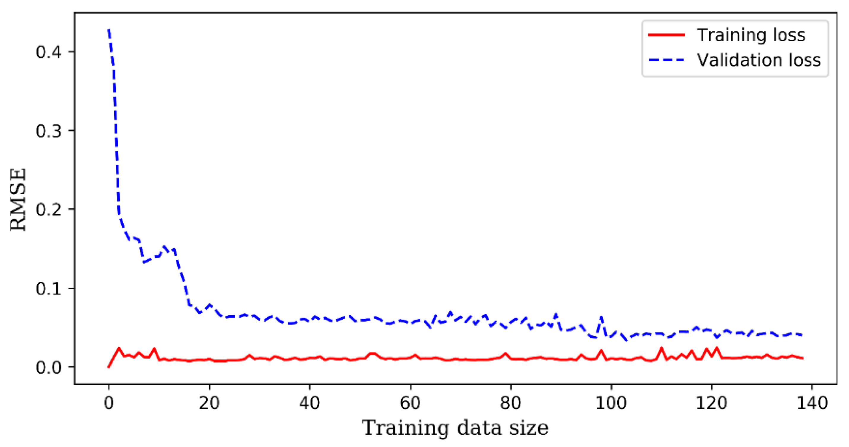
An ANN model is trained with the training data and validated with the test data. Figure 14 shows the learning rate curves of an ANN model at $T_E=5 \mathrm{s}$ which indicates the performance of the model on the training and validation as a function of the size of the training data. The value of the loss function (root mean squared error) is initially zero and starts to go up as the size of the training data increases. However, it will finally reach a low plateau, where adding new data points to the training dataset does not make the averaged error better or worse. Likewise, the ANN model is not capable of being generalized properly at the initial stage, that is the reason why the validation error is quite large.

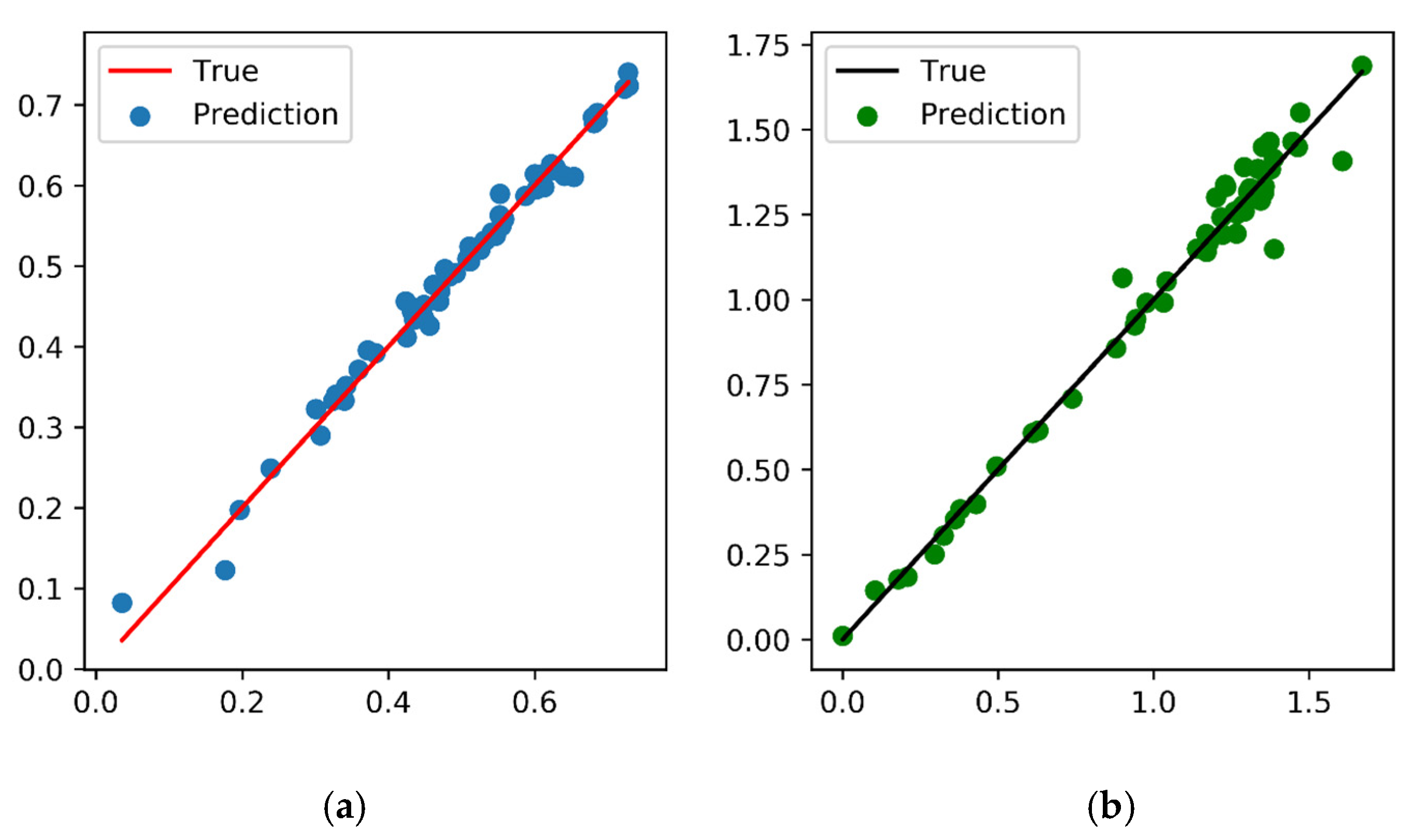
After training the ANN model with the training data, the conversion efficiency (${\eta }_{irr}$) and non-dimensional significant wave force (${\left(f_1\right)}_{1/3}/\rho g{d}_{1}A$) on the barrier are predicted with the test data. The resulting predictions are compared with the true values. The deviation of the predicted values(circle) from the true values(line) is shown in Figure 15 and a good agreement between them is observed.

To further verify the accuracy of the ANN model, three error metrics are used; mean squared error (MSE), mean absolute error (MAE), and $R^2$ score. The mean squared error (MSE) and mean absolute error (MAE) with $L$ sample points in the test data are defined as

$$\begin{array}{l}\mathrm{MSE}(y,\widehat{y})=\frac{1}{L}{\displaystyle {\displaystyle \sum }_{i=0}^{L-1}}{(y_i-{\widehat{y}}_i)}^2,\\ \mathrm{MAE}(y,\widehat{y})=\frac{1}{L}{\displaystyle {\displaystyle \sum }_{i=0}^{L-1}}\left|y_i-{\widehat{y}}_i\right|.\end{array}$$

(40)

The $R^2$ score provides an indication of goodness of fit and therefore a measure of how well unseen samples are likely to be predicted by the present model. The estimated $R^2$ score is defined as:

$$R^2(y,\widehat{y})=1-\frac{{\displaystyle \sum _{i=1}^L{(y_i-{\widehat{y}}_i)}^2}}{{\displaystyle \sum _{i=1}^L{(y_i-\overline{y})}^2}}$$

(41)

where the upper bar denotes a mean value.

The error metrics for two output features are given in

Table 2. Error metrics of two output features for three different energy periods.

	${\mathit{T}}_{\mathit{E}}=\mathbf{4} \mathbf{s}$		${\mathit{T}}_{\mathit{E}}=\mathbf{5} \mathbf{s}$		${\mathit{T}}_{\mathit{E}}=\mathbf{6} \mathbf{s}$
Error Metrics	${\mathit{\eta }}_{\mathit{i}\mathit{r}\mathit{r}}$	$\frac{{\left({\mathit{f}}_{\mathbf{1}}\right)}_{\mathbf{1}/\mathbf{3}}}{\mathit{\rho }\mathit{g}{\mathit{d}}_{\mathbf{1}}\mathit{A}}$	${\mathit{\eta }}_{\mathit{i}\mathit{r}\mathit{r}}$	$\frac{{\left({\mathit{f}}_{\mathbf{1}}\right)}_{1/3}}{\mathit{\rho }\mathit{g}{\mathit{d}}_{\mathbf{1}}\mathit{A}}$	${\mathit{\eta }}_{\mathit{i}\mathit{r}\mathit{r}}$	$\frac{{\left({\mathit{f}}_{\mathbf{1}}\right)}_{\mathbf{1}/\mathbf{3}}}{\mathit{\rho }\mathit{g}{\mathit{d}}_{\mathbf{1}}\mathit{A}}$
MSE	0.0005	0.006	0.0004	0.003	0.0005	0.003
MAE	0.016	0.054	0.015	0.034	0.013	0.028
score	0.981	0.945	0.987	0.979	0.951	0.991

. If judging with the MSE and MAE value close to 0, and $R^2$ score close to 1.0, the present ANN models have a good prediction accuracy and meet the engineering requirement.

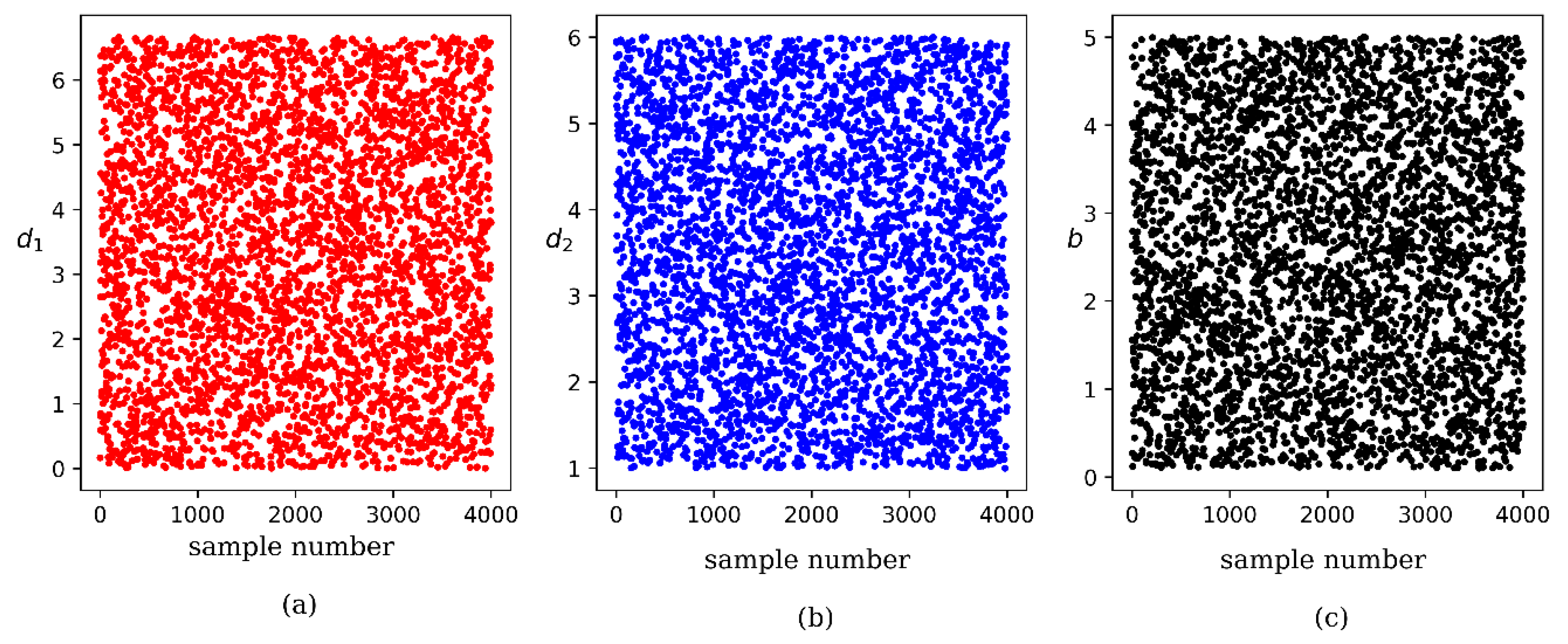
To obtain optimal design features, the predictions are carried out using the trained ANN model with a large dataset. The database used for predictions is made with the LHS methodology containing 4000 samples. The sample points are distributed uniformly within the given bounds for each input feature (see Figure 16).

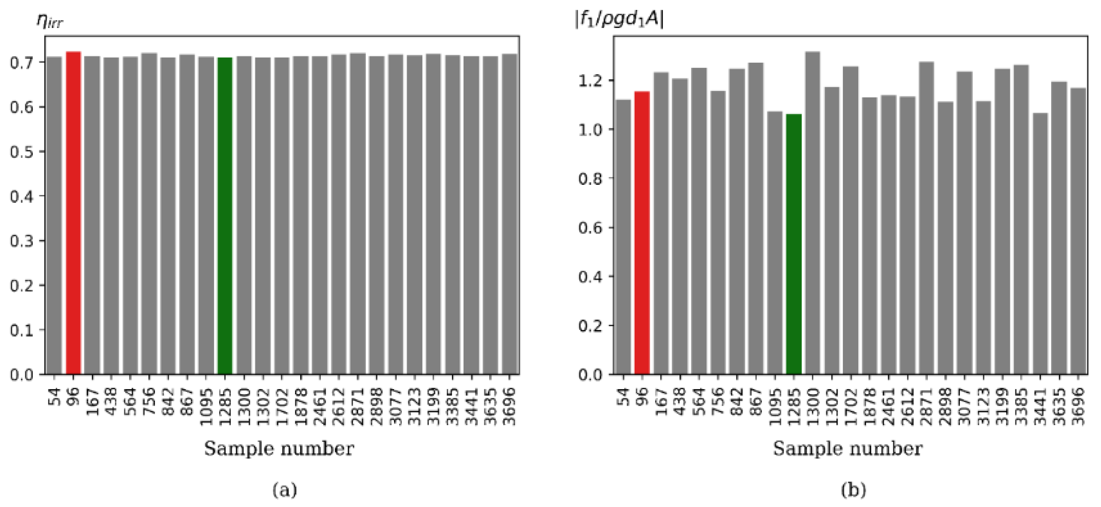
Since we already have a trained ANN model, the prediction of the output features for this large dataset is quite easy. From the predictions, we choose 25 combinations of design features that yield high conversion efficiency. Figure 17 shows the bar plots for conversion efficiency (${\eta }_{irr}$) and non-dimensional significant wave force (${\left(f_1\right)}_{1/3}/\rho g{d}_{1}A$) at these combinations for a fixed energy period of 5 s. The maximum predicted conversion efficiency is about 0.723 (marked in red) and the corresponding predicted value of significant wave force is 1.15. The significant wave force can be reduced by 8% at another combination (marked in green) and the conversion efficiency for this combination is 0.71, slightly less (1.8%) than the maximum value (0.723). When considering both the structural safety of a bottom-mounted vertical barrier and conversion efficiency as similar weighting, the latter combination can be taken as optimal design features. However, this kind of decision can vary depending on the designer’s preference in weighting.

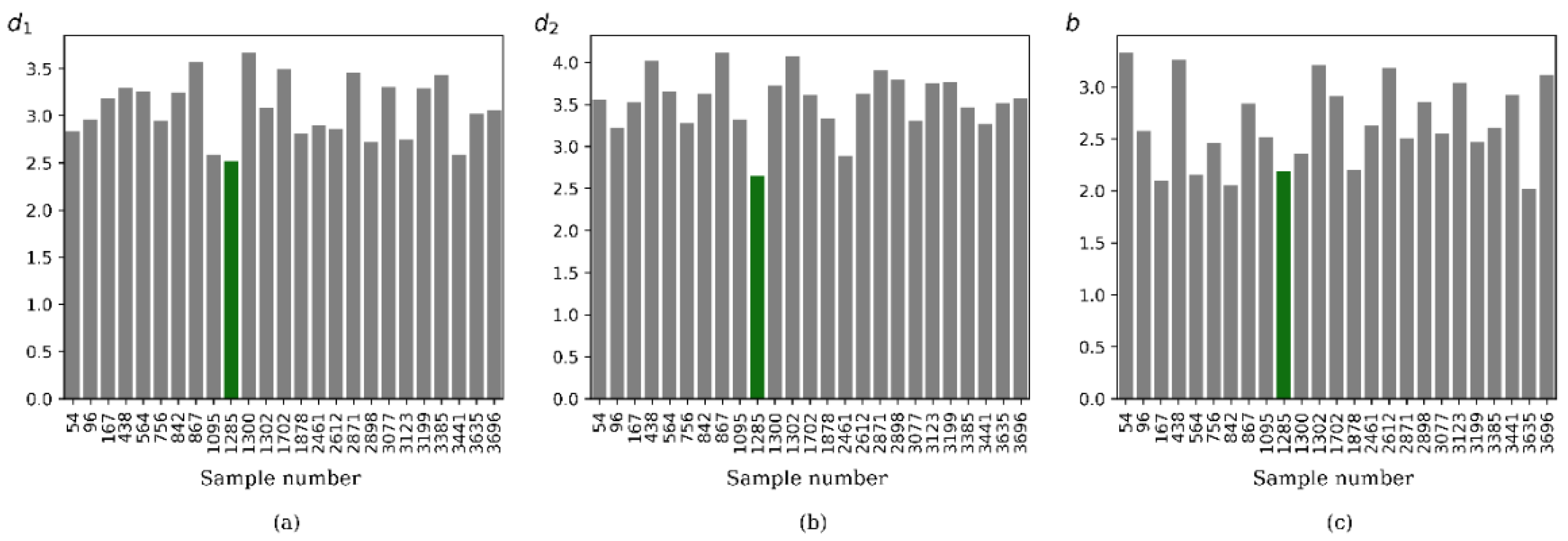
The optimal geometric values of $d_1$,$d_2$, and b belonging to this combination (marked in green) are about 2.51 m, 2.65 m, and 2.18 m, respectively (Figure 18). The same methodology is followed for the remaining energy periods $T_E=4.6\hspace{0.17em}\mathrm{s}$ and the optimal geometric values of the U-OWC are summarized in

Table 3. Optimal geometric values of the U-OWC for different energy periods.

${\mathit{T}}_{\mathit{E}}\left(\mathbf{s}\right)$	${\mathit{d}}_{\mathbf{1}}\left(\mathbf{m}\right)$	${\mathit{d}}_{\mathbf{2}}\left(\mathbf{m}\right)$	$\mathit{b}$	${\mathit{\eta }}_{\mathit{i}\mathit{r}\mathit{r}}$	$\frac{{\left({\mathit{f}}_{\mathbf{1}}\right)}_{1/3}}{\mathit{\rho }\mathit{g}{\mathit{d}}_1\mathit{A}}$
4	0.268	1.065	2.282	0.773	0.257
5	2.518	2.650	2.187	0.710	1.060
6	3.188	4.715	3.912	0.723	1.050

following the same design procedure.

5. Conclusions

Using a developed analytical model (MEEM) based on linear potential theory, it is found that there exist two resonance peaks in the power-extraction (or conversion efficiency) curve of a U-OWC device. The first resonance is associated with the piston-mode resonance inside the chamber, while the second spike-like resonance is caused by the similar fluid motion between the barrier and chamber wall. The combination of two peaks helps to expand the range of high wave-energy conversion. The corresponding wave forces on the front barrier are also computed from the analytic solutions. It is shown that a U-OWC with a barrier height of $d_1$ = 2.0 m has a maximum conversion efficiency of 0.70, which is higher than that (=0.56) of a conventional OWC with no-barrier ($d_1$ = 0 m) in irregular waves.

Subsequently, the optimal design of the U-OWC is determined by using a machine learning method. In this regard, three input features, the vertical barrier geometry (height, distance) and submergence depth of the chamber wall, and two output features, the conversion efficiency and wave forces on a front barrier, are chosen. Using the analytical model described in Section 2, the database from randomly distributed input and output features is created using Latin hypercube sampling (LHS). From the feature study on the database, it is observed that there exists a strong correlation between barrier height and the output features. The present ANN model is shown to be trained well with $R^2$ score of 0.95 even if a database is comparatively small in size (200 samples). Using the trained ANN model, the optimal geometric values of $d_1$,$d_2$, and b are predicted to be 2.51 m, 2.65 m, and 2.18 m from a large dataset (4000 samples) in irregular waves with $T_E$ = 5 s.

The developed ANN model can supply guidelines in determining the optimal design values of a U-OWC suitable to wave conditions at the installation site. The present design tool based on an ANN model is especially valuable when the number of input features is large.

The analytical model is based on a potential theory, therefore, it cannot take into account energy dissipation by the formation of vortices at the ends of the barrier and chamber wall. Therefore, the conversion efficiency and wave forces may overestimate the actual values. To consider the viscous effects in the design of a U-OWC, either the numerical simulations by CFD codes or physical experiments need to be paralleled as a supplementary measure of the present analytical model.

References

- Salter, S. Wave power. Nature 1974, 249, 720–724. [Google Scholar] [CrossRef]
- Masuda, Y. Experimental full-scale results of wave power machine KAIMEI in 1978. In Proceedings of the 1st Symposium on Wave Energy Utilization, Gothenburg, Sweden, 30 October–1 November 1979; pp. 349–363. [Google Scholar]
- Evans, D.V.; Porter, R. Hydrodynamic characteristics of an oscillating water column device. Appl. Ocean Res. 1996, 15, 155–164. [Google Scholar] [CrossRef]
- Martins-Rivas, H.; Mei, C.C. Wave power extraction from an oscillating water column along a straight coast. Ocean Eng. 2009, 36, 426–433. [Google Scholar] [CrossRef]
- Zheng, S.; Antonini, A.; Zhang, Y.; Greaves, D.; Miles, J.; Iglesias, G. Wave power ex-traction from multiple oscillating water columns along a straight coast. J. Fluid Mech. 2019, 878, 445–480. [Google Scholar] [CrossRef]
- Deng, Z.; Wang, L.; Zhao, X.; Wang, P. Wave power extraction by a nearshore oscillating water column converter with a surging lip-wall. Renew. Energy 2020, 146, 662–674. [Google Scholar] [CrossRef]
- Wang, R.Q.; Ning, D.Z. Dynamic analysis of wave action on an OWC wave energy converter under the influence of viscosity. Renew. Energy 2020, 150, 578–588. [Google Scholar] [CrossRef]
- Heath, T.; Whittaker, T.J.T.; Boake, C.B. The design, construction and operation of the LIMPET wave energy converter (Islay, Scotland). In Proceedings of the Fourth European Wave Power Conference; Energy Centre Denmark, Danish Technological Institute: Tastrup, Denmark, 2000; pp. 49–55. [Google Scholar]
- Hong, K.; Shin, S.H.; Hong, D.-C.; Choi, H.S.; Hong, S.W. Effects of shape parameters of OWC chamber in wave energy absorption. In Proceedings of the Seventeenth International Offshore and Polar Engineering Conference, Lisbon, Portugal, 1–6 July 2007; pp. 428–433. [Google Scholar]
- Boccotti, P. On a new wave energy absorber. Ocean Eng. 2003, 30, 1191–1200. [Google Scholar] [CrossRef]
- Boccotti, P.; Filianoti, P.; Fiamma, V.; Arena, F. Caisson breakwaters embodying an OWC with a small opening—Part II: A small-scale field experiment. Ocean Eng. 2007, 34, 820–841. [Google Scholar] [CrossRef]
- Malara, G.; Arena, F. Analytical modeling of a U-Oscillating water column and performance in random waves. Renew. Energy 2013, 60, 116–126. [Google Scholar] [CrossRef]
- Malara, G.; Gomes, R.P.F.; Arena, F.; Henriques, J.C.C.; Gato, L.M.C.; Falcão, A.F.O. The influence of three-dimensional effects on the performance of U-type oscillating water column wave energy harvesters. Renew. Energy 2017, 111, 506–522. [Google Scholar] [CrossRef]
- Malara, G.; Arena, F. Response of U-Oscillating Water Column arrays: Semi-analytical approach and numerical results. Renew. Energy 2019, 111, 1152–1165. [Google Scholar] [CrossRef]
- Ning, D.; Guo, B.; Wang, R.; Vyzikas, T.; Greaves, D. Geometrical investigation of a U-shaped oscillating water column wave energy device. Appl. Ocean Res. 2020, 97. [Google Scholar] [CrossRef]
- Hill, T.; Marquez, L.; O’Connor, M.; Remus, W. Artificial neural network models for forecasting and decision making. Int. J. Forecast. 1994, 10, 5–15. [Google Scholar] [CrossRef] [Green Version]
- Wójcik, P.I.; Kurdziel, M. Training neural networks on high-dimensional data using random projection. Pattern Anal. Appl. 2019, 22, 1221–1231. [Google Scholar] [CrossRef] [Green Version]
- Lawrence, S.; Giles, C.L.; Tsoi, A.C.; Back, A.D. Face recognition: A convolutional neural-network approach. IEEE Trans. Neural Netw. 1997, 8, 98–113. [Google Scholar] [CrossRef] [PubMed] [Green Version]
- Dahl, G.E.; Yu, D.; Deng, L.; Acero, A. Context-dependent pre-trained deep neural networks for large-vocabulary speech recognition. IEEE Trans. Audio Speech Lang. Process. 2012, 20, 30–42. [Google Scholar] [CrossRef] [Green Version]
- Rifaioglu, A.S.; Atas, H.; Martin, M.J.; Cetin-Atalay, R.; Atalay, V.; Doǧan, T. Recent applications of deep learning and machine intelligence on in silico drug discovery: Methods, tools and databases. Brief. Bioinform. 2019, 20, 1878–1912. [Google Scholar] [CrossRef]
- Sarkar, D.; Contal, E.; Vayatis, N.; Dias, F. Prediction and optimization of wave energy converter arrays using a machine learning approach. Renew. Energy 2016, 97, 504–517. [Google Scholar] [CrossRef]
- Deberneh, H.M.; Kim, I. Predicting output power for nearshore wave energy harvesting. Appl. Sci. 2018, 8. [Google Scholar] [CrossRef]
- Masoumi, M. Ocean data classification using unsupervised machine learning: Planning for hybrid wave-wind offshore energy devices. Ocean Eng. 2021, 219. [Google Scholar] [CrossRef]
- McKay, M.; Beckman, R.; Conover, W. A comparison of three methods for selecting values of input variables in the analysis of output from a computer code. Technometrics 1979, 21, 239–245. [Google Scholar]
- Ghawi, R.; Pfeffer, J. Efficient Hyperparameter Tuning with Grid Search for Text Categorization using kNN Approach with BM25 Similarity. Open Comput. Sci. 2019, 9, 160–180. [Google Scholar] [CrossRef]
- Kessler, T.; Dorian, G.; Mack, J.H. Application of a rectified linear unit (RELU) based artificial neural network to cetane number predictions. In Proceedings of the ASME 2017 Internal Combustion Engine Division Fall Technical Conference, Seattle, WA, USA, 15–18 October 2017; pp. 1–8. [Google Scholar] [CrossRef] [Green Version]
- Saputro, D.R.S.; Widyaningsih, P. Limited memory Broyden-Fletcher-Goldfarb-Shanno (L-BFGS) method for the parameter estimation on geographically weighted ordinal logistic regression model (GWOLR). AIP Conf. Proc. 2017, 1868. [Google Scholar] [CrossRef] [Green Version]
Figure 1.
Schematic sketch of a U-OWC device.
Figure 2.
Comparison of flux by the incident waves (a), radiation conductance (b), and radiation admittance (c) for .
Figure 3.
Induced flux by the incident waves (a), radiation conductance (b), and radiation admittance (c) as a function of the barrier height () for .
Figure 4.
Non-dimensional wave forces on the barrier (a) and chamber wall (b) as a function of the barrier height () for .
Figure 5.
Optimal turbine constant as a function of the barrier height () for .
Figure 6.
Extraction power (a), and conversion efficiency (b) at the optimal turbine constant as a function of the barrier height () for .
Figure 7.
Conversion efficiency of a U-OWC device at the optimal turbine constant as a function of the submergence depth of the chamber wall (a) and barrier distance (b) for .
Figure 8.
Conversion efficiency (a) and non-dimensional wave force (b) on a barrier as a function of the barrier height () and energy period in irregular waves for , .
Figure 9.
Scatter diagrams of the samples of input feature: (a) barrier height, (b) submergence depth of a chamber wall, and (c) barrier distance.
Figure 10.
Variation of conversion efficiency of a U-OWC versus input feature: (a) barrier height, (b) submergence depth of a chamber wall, and (c) barrier distance at TE = 5 s in irregular waves.