Multi-Level Optimization Process for Rationalizing the Distribution Logistics Process of Companies Selling Dietary Supplements

Abstract

The commission sales form is a very significant channel of sales today, which is especially true in the field of dietary supplements. In parallel, the prevailing digitalization trends have opened up further new opportunities for this form of distribution. The multi-level optimization process presented in the publication makes it possible to optimize the distribution logistics processes of companies producing food supplements at a high level by exploiting these new possibilities. The operation of the procedure is also illustrated through a practical example.

1. Introduction

Today, the proper development of supply chains plays an important role in maintaining the competitiveness of companies. The development and operation of supply chains is dealt with in detail in the international literature, but at the same time there are types of supply chains whose development possibilities have been overshadowed. Since the number of products offered by commercial companies and pharmacy offerings is now significant, commission sales are one of the most permeable ways to get on the market. Production and distribution companies are constantly competing with each other, resulting in competition, so cost reduction has become vital.

The spread of commission sales was made possible by the development of the Internet, the reduction of telecommunications costs and the development of IT applications. Digitalisation is not only about technology, but also about the strategy companies have, their ability to adapt to changed environmental conditions, the ability to adapt rapidly to different technologies in order to remain competitive, and whether SMEs (small and medium-sized enterprises) have learning skills [1]. In the past, the development of transport enabled commission sales to start, whereas nowadays this is induced by information communications technologies [2].

This publication focuses on the distribution side of supply chains of companies producing commissioned dietary supplements as perhaps the most important sub-area for commission sales. The main objective is to describe a multilevel optimisation process that can make a significant contribution to increasing the efficiency of the distribution side in the supply chains that are sold in a commissioned way through coordinated management of inventory and transport aspects.

Following the introduction, the paper uses the method of systematic literary research to explore scientific literature on existing supply chain operational strategies, supplemented by a statistical summary of search results. Section 3, following the literature research, presents the distribution models defined by the authors during the research, and then the fourth section describes the return models defined. In Section 5, the entire system model, on which the optimization process is based, is presented. The multilevel optimisation process itself is described in detail in Section 6 thereafter. Then, in Section 7, the method is presented by solving a problem that is close to practice. Finally, Section 8 contains the summary and the debate section.

2. Literature Research

The supply chain describes flow processes across organizations. Companies have either an explicit strategy or an implicit strategy relevant to the manager. However, given the increasingly widespread view that supply chains, rather than individual companies, compete with each other, it is natural that these organizational strategies are coordinated and that the objectives and the means assigned to them are also set at supply chain level [3]. The supply chain strategy should be formulated mainly for companies that play a guiding role and operate as central companies in their supply chains, since because of their position of power they will primarily shape the operational structure and processes of the given supply chain. At the same time, it is also a limit for them to know in what environment, under what conditions, and with what partners they can work.

Companies face a number of challenges in seeking to optimize and harmonize their supply chain [4].

The starting point for literary research in the field is the definition of keywords related to the topic. Since dietary supplements are considered food with a shelf life, research focuses on supply chain strategies that are limited to food. In literature research, the following keywords were used in search:

• supply chain
• operational strategy
• food

In order to delimit the literature more closely related to the research topic, it was necessary to narrow the search for original keywords by searching for the keywords “supply chain AND operational strategy” in combination. After that, the search results for each keyword resulted in sufficiently relevant results, with 3080 publications aggregating WoS, Scopus, and ScienceDirect search results. Adding the search keywords “supply chain AND operational strategy” to the keyword “food” greatly reduced the search results set. The evolution of the chronological volume of publications is shown in Figure 1, where there is an increasing trend year after year, so it can be considered a relevant field of research:

Figure 2 illustrates the weight of the different disciplines in the publication list of the Scopus database based on data from the last 20 years. From this, it can be observed that the delimited field of research also has a multidisciplinary character, since not only disciplines related to engineering activities can be observed, but research related to management and decision support is also significant. The data show that few people from a logistical aspect examine the area.

In the Scopus database, a complex search for the keywords “supply chain, operational strategy” has been carried out on the basis of data from the last 10 years, as a result of which the proportion of keywords not yet examined (Figure 3) has been examined for 1229 publications. It can be concluded that the terms green supply chain, cost, logistics, and production also play a prominent role in the works.

As a further analysis of the delimited set of studies, the 10 most published persons on the subject were selected (

Table 1. The 10 most published authors in the Scopus scientific library for “supply chain, operational strategy” keywords between 2010 and 2020 [Source: Self-editing].

Author	Published Papers	Author	Published Papers
Chen, Z.	8	Jajja, M.S.S.	5
Smith, A.D.	8	Laosirihongthong, T.	5
Gunasekaran, A.	6	Sarkis, J.	5
Wang, X.	6	Ahmed, W.	4
Cannella, S.	5	Brun, A.	4

). The analysis shows that the number of authors involved in the publication of five or more articles can only be estimated at eight people.

The following summary analysis was prepared, focusing on food authors and the most cited publications, after processing 3080 works delimited as a result of systematic literature research.

In 2015, Vlachos discussed the food supply chain of SMEs (small and medium-sized enterprises) in a case study. The study notes that the majority of food companies are small and medium-sized enterprises and develop a lean-based action plan based on a tea company. It develops a three-step action plan to highlight how cost-effective ‘slender’ thinking can be applied in the food sectors [5].

In 2019, Kambele and co-authors published one of the tools in Industry 4.0, the Internet of Things (IoT) for small and medium-sized enterprises. They note that IoT can provide significant assistance to SMEs in the supply chain in controlling food quality, controlling their shelf life, and planning waste management and recycling logistics for expired products [6].

Afonso and Cabrita published about the lean supply chain in 2015. They argue that lean supply chains are striving at the operational level to optimize supply chain processes, seek simplification, reduce waste, and reduce non-value-adding activities. Their research aims to develop a lean supply chain management conceptual framework for a food SME [7].

In 2017, Pariazar and his co-authors developed a two-step stochastic programming model to explore trade-offs between costs and risk factors to establish a food supply chain. They also present a number of calculation results in their article [8].

In 2020, Ortiz-Barrios et al. discussed the whiplash effect of the food supply chain. Consequently, they wrote about delays in production schedules, poor customer contact, excessive stockpiling, and misplaced capacity planning. In their paper, they proposed a hybrid approach to a mixture of AHP, DEMATEL and TOPSIS methods [9].

Many publications are trying to find a solution from different approaches to how to reduce or eliminate food losses within the supply chain [10,11,12].

In 2017, Sreedevi and Saranga discussed how companies are indulging in expanding their product offerings in order to remain competitive, creating vulnerabilities in the supply chain. Due to supply chain uncertainty, companies are facing increasing risks in terms of production and distribution, which ultimately leads to poor operating performance. Their empirical analysis concludes that supply and production flexibility helps to reduce the risks to the supply and production process [13].

In 2015, Dobos and Gelei published about corporate inventory management for a pharmaceutical company. They note that the company’s fundamental objective is to significantly reduce the level of inventory investment while maintaining an adequate level of service. To achieve this, elements of classic stockpiling mechanisms are combined [14].

In 2018, Sabouhi and his co-authors will publish on the main goals of a pharmaceutical supply chain, reducing risks and costs, maintaining market share and consumer satisfaction. An integrated hybrid approach is presented to help planning supply chain flexibility [15].

In 2017, Li et al. developed a game theory decision-making method for production and procurement in a decentralized supply chain consisting of a manufacturer and a retailer. The demand for the product is random and the production yield of the manufacturer is stochastic. An analysis was carried out on how these factors affect each other’s operational strategies and performance [16].

Daniela A. and Maria G. studied some complex distribution design issues in 2005, which include placement, warehousing, transportation, and inventory decisions. As one possible solution to the problem, the Perl and Daskin models are proposed [17].

In 2008, Claassen and his team examined the benefits of VMI and the success factors or prerequisites needed for effective application. The most important thing for the commissioner was assumed to be that its production could be carried out on the basis of real customer demand, thereby being able to smooth out fluctuations and carry out its tasks proactively in the light of accurate demand data [18].

In 2014, Zanoni, Jaber and Mazzoldi presented a unique supply chain model for coordinated inventory supply decisions within the framework of the VMI system, which is implemented on the basis of a two-tier supply chain system, with a commission transmitter and a single commissioner [19].

In 2010, Chen and his co-authors addressed the problem of coordinating a vertically segregated distribution system for commission sales in two-tier distribution chains. They formulate the profit maximisation problem and carry out equilibrium analysis in cooperative and non-cooperative conditions. An income-sharing scheme is then proposed [20].

Bieniek discussed commission sales in 2018, where market demand is additive, linearly price-dependent, and uncertain. Taking into account uncertain return behaviour in a commission contract, in an additive random demand framework, the risk analysis is examined and an answer is sought as to how buyer yield uncertainty and other model parameters affect decision variables [21].

In 2013, Hariga and his co-authors examined a supply chain consisting of a commission tax and several commissions in a two-tier supply chain. The supply chain operates on the basis of a VMI contract that sets limits on the stock level of retailers. The problem of synchronizing the seller’s cycle time with unequal order cycles for buyers is addressed by developing a whole number of nonlinear programmes that minimise common relevant inventory costs, in addition to storage restrictions [22]. In 2017, Zahran and his co-authors examined a three-tier supply chain model consisting of commissioning, commissioner and customers, unlike the two-tier supply chain, which is found in large numbers in the literature. It examines several coordination cases, but the possibility of direct material flow between commissions and the relationship of the central company with customers are not reflected here either [23].

In several publications, it is mentioned that the growing product structure along with increasing customer demands and expectations pose unexpected challenges to the operating systems of company supply chains. Such challenges require the development of new and innovative flexibility concepts and models [13,24,25,26,27].

It can be concluded that the operational strategy of the supply chains that sell commissions is covered by a number of publications, but at the same time no commissioned supply chain model has been developed that would take into account the possibilities of material flow between commissioners and the recycling of materials generated by commissions, while minimizing the stock levels and transport costs of the finished product.

3. Description of the Defined Distribution Models

For the distribution model variants developed (Figure 4), a uniform marking system has been applied to the markings, where:

• $V_k$: k buyer ($k=1,2,\dots ,o$),
• $R_f$: f warehouse ($f=1,2\dots ,d$),
• $E_h$: h distribution group warehouse ($h=1,2,\dots ,g$),
• EK: central distribution warehouse,
• $Bi{z}_j$: j commissioner ($j=1,2,\dots ,m$).

Figure 4 shows three types of arrows. Black arrows represent the material flow of the base model, while other supplemented versions of which are marked with blue and green arrows. In addition, an integrated version of all types can be formed.

• D1, D2, D3, D1–D3: For this type of distribution model, a unique warehouse is assigned to each commission member and through it receives inventory replacements from the central commissioner. The advantage of the model is that commissioned workers can quickly get the necessary products from a separate warehouse reserved for them, but the disadvantage of the system is that many warehouses have to be built and/or maintained and operated. In the D1 base model, commissioners do not have material flow and commissioners have unique customers. With the addition of D2 to the basic model, it is possible to implement the material flow among the commissions. In addition to the base model D3, the customer relationships of commissioners can be combined. The D1-D3 model contains all the material flow relationships of the D1 base model and its additions.
• D4, D5, D6, D4–D6: For distribution models of this type, some commissioners are assigned to a specific warehouse based on certain criteria (location, product structure, etc.), i.e., each warehouse has a specific group of commissions. In this case, several commissions are supplied from a given warehouse. The number of warehouses was less than for the D1-D3 models, which, overall, could mean cost savings during operation. In the D4 base model, there is no material flow between commissions and commissioners have unique customers. With the addition of D5 to the basic model, it is possible to implement the material flow among the commissions. In addition to the base model D6, the customer relationship system of commissioners can be combined. Model D4–D6 contains all material flow connections of the D4 base model and its additions.
• D7, D8, D9, D7–D9: For these distribution models, the logistics and production plant which is the central commission delivers the products directly to the commissioners through a central distribution warehouse. Since warehousing takes place in a distribution central warehouse, a complex material and information flow connection between the central distribution warehouse and the commissions is necessary for the proper functioning of the warehouse. The advantage is that only one central warehouse has to be operated, but the disadvantage is that all commission and customer needs must be handled from here. In the D7 base model, commissioners do not have material flow and commissioners have unique customers. With the addition of the basic model D8, it is possible to implement the material flow among the commissions. In addition to the base model D9, the customer relationship system of commissioners can be combined. Model D7–D9 contains all material flow connections of the D7 base model and its additions.
• D10, D11, D12, D10–D12: For distribution models of this type, distribution is performed directly from the logistics and production plant that delivers it to the central commission. There is no excessive warehousing activity in the logistics and production plant that is the central commission. Therefore, supplemented by the storage activity in the commission distribution warehouses, it is necessary to store quantities that meet the continuous commission and customer needs, which are often carried out in the size of the storage space in the commission sales space. This requires a more advanced material and information flow link, both between the logistics and production plant in the central commission and between commissioners and customers. In the D10 base model, there is no material flow between commissions and commissioners have unique customers. With the addition of the basic model D11, it is possible to implement the material flow among the commissioners. In addition to the base model D12, the customer relationship system of commissioners can be combined. Model D10-D12 contains all material flow connections of the D10 base model and its additions.
• D13, D14, D15, D13–D15: Distribution models of this type are made up of mixed uses of the previous four models. There are commissions who receive the products directly from the commissioner, there are commissioners who receive the replacement products directly in individual warehouses, and there are commissions that are assigned to different groups and these groups receive the replacement products through a single warehouse. In the D13 base model, there is no material flow between commissions and commissioners have unique customers. With the addition of the basic model D14, it is possible to implement the material flow among the commissioners. In addition to the base model D15, the customer relationship system of commissioners can be combined. Model D13–D15 contain all material flow connections of the D13 base model and its additions.

Overall, there are 20 distributional parent flow models on the commission and customer side.

4. Description of the Defined Return Models

Figure 5 shows the return model variants, which have the following marking system:

• $R_f$: f warehouse ($f=1,2,\dots ,d$),
• $E_h$: a h return group warehouse ($h=1,2,\dots ,g$),
• EK: central return warehouse,
• $Bi{z}_j$: j commissioner ($j=1,2,\dots ,m$).

Figure 5 shows two types of arrows. Black arrows represent the material flow of the base model, a further supplemented version of which is marked with a green arrow.

• V1, V2: For this type of return model, each commission is assigned to a separate individual return warehouse and through it the return material flows to the central commissioning plant. The advantages of the model are that commissioned customers can handle return quantities in a unique warehouse assigned to them, but the disadvantage of the system is that many warehouses have to be operated. In the V1 base model, there is no flow of material between commissions. With the addition of the base model V2, it is possible to implement the material flow among the commissioners, so that the centre can select a unique warehouse where it can store all the returned products.
• V3, V4: For this type of return models, commissioners are assigned to a specific return warehouse based on certain criteria (location, product structure, etc.), i.e., each return warehouse has a specific group of commissions. The capacity of a group warehouse shall be distributed among several commissions in respect of returned products. The number of warehouses is less than for V1 and V2 models. Overall, this can mean cost savings for operation. In the V3 base model, there is no material flow between commissions. With the addition of the V4 of the basic model, it is possible to implement the material flow among the commissioners, so that the centre can select a group warehouse where it can store all the returned products.
• V5, V6: For these return models, returned products from commissions are shipped to a central warehouse. The central warehouse is used jointly by the commissions. In order for the warehouse to function properly, a complex material and information flow relationship is required between the central warehouse and the commissions. The advantage is that only necessary to operate one warehouse, but the disadvantage is that necessary to be able to manage all commission return stocks. In the V5 base model, there is no flow of material between commissions. With the addition of the V6 of the basic model, it is possible to carry out the flow of materials among the commissions, so that the products intended for return can be grouped among the commissions, even at a commission with a larger warehouse, up to a certain amount.
• V7, V8: For this type of return model, the return will be made directly to the logistics and production plant that has delivered it directly to the central commission. This requires a more advanced material and information flow link, both between the logistics and production plant that provides the central commission, and between commissioners and customers. In the V7 base model, there is no material flow between commissions. With the addition of the V8 of the basic model, it is possible to carry out the flow of materials among the commissions, so that the products intended for return can be grouped among the commissions, even at a commission with a larger warehouse, these products can be stored up to a certain amount.
• V9, V10: Distribution models of this type are made up of mixed uses of the previous four models. There are commissions from whom products flow directly back, there are commissions from whom products flow directly back from their own warehouse, and there are commissions that are assigned to different groups and from each of these groups they carry out the flow of return material using a warehouse. In the V9 base model, there is no material flow between commissions. In addition to the V10 of the basic model, it is possible to implement the flow of materials among the commissions, so that the return capacities can be distributed to a unique, group, central warehouse, or, when transferred to a commission, the products designated for return can be returned directly to the centre.

From the commission side, 10 types of return material flow models can be distinguished. The main difference between these models from the general supply chain types is that the recovery of products to be regrouped or expired is contrary to the general material flow.

For the previously explored model variants, 20 variants were discovered for commission distribution model variants and 10 variants for commission return model variants. In addition, five different versions of the procurement model can be identified, but these have not been detailed in the context of this publication. A combination of these variants can describe 1000 different four-level commission supply chains.

Information flow links are extremely diverse. In general, there should be no information flow relationship between the commissioner and the buyer, as well as between the raw material supplier and the commission and the customer, but this may occur in the relations of the other objects, depending on the case.

5. Understanding the Delimited System Model

Based on the models presented, commissioned systems can be extremely diverse and specific, but it is essential to define a general test model for the development of test methods that can be flexibly modified according to company needs, thus giving scope for testing all variants if necessary. It can be said that the model described in Figure 6 meets these requirements, as it also includes the possibility of transport between commissions and the flow of materials related to the recycling of products with expired warranties. In the light of this line of thought, the basic model D12, V8 was selected, coupled directly with the supply to the logistics and production plant that provided the central commission. The entire model is shown in Figure 6.

The typical logistics process of the selected supply chain model can be summarized as follows. Suppliers deliver the raw materials for production directly to the logistics and production plant that delivers them to the central commission. The central logistics and production plant providing the commission comprises the areas of raw material storage, production, finished product storage, and picking, between which the flow of materials and information is usually controlled by corporate governance systems (for example SAP, FOSS, etc.). In the case of distribution and return models, connections without direct distribution storage have been established, the operation of which is described in the model variants D12, V8.

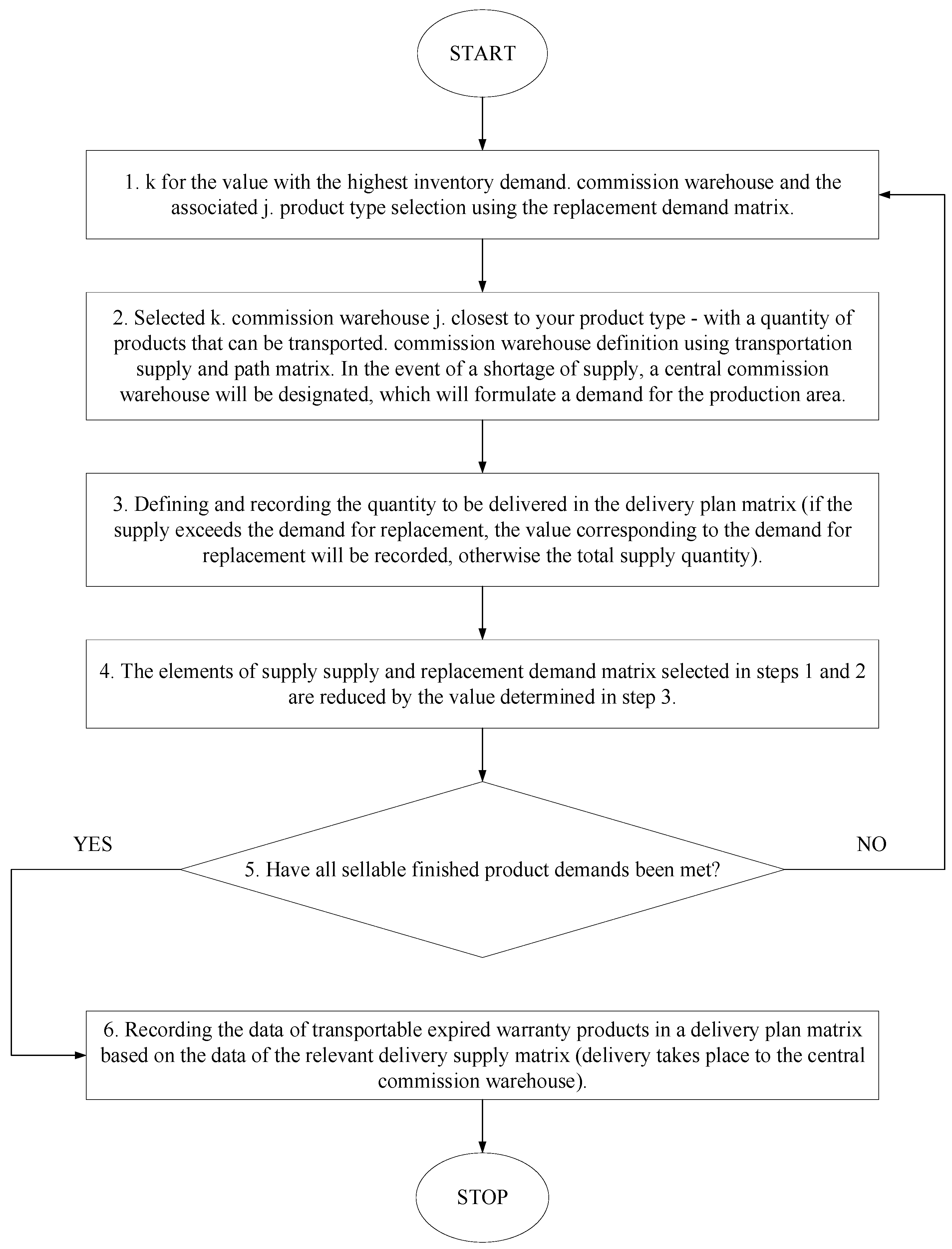
6. Presentation of the Optimization Process Developed

Based on the model described in Figure 6 of the company producing and distributing food supplements, an optimization process has been developed to minimize the level of stock in the distribution logistics system and transport costs. In addition, the optimization process focuses on reducing the volume of expired products and defining their recycling system.

A procedure has been developed to meet all customer needs while minimizing the stock level of the entire finished product, as well as the possibility of transport between commissioned persons. As a result of optimization, transport relationships and related transport quantities to minimize handling work are defined for each day. The detailed process of optimization (Figure 7) is described below.

Process description:

1. Determination of the investigation period: The time horizon of the study should be determined in this step. It is assumed that during the designated future time horizon, the stock fall mechanisms defined at the beginning of the time horizon may not change. However, at the end of the period under review, they may be adjusted based on factual data, the results of which can be taken into account in the next period.

2. Determination of the distance between objects in material flow relationship: The length of the transport routes between the central commission warehouse (k = 1) and the commission warehouses and the commission warehouses (k, k’) is included in the road matrix (1).

$$U^E=\left[u_{k,k\prime }^E\right],\mathrm{where}k=1,2,\dots ,p; k’=1,2,\dots ,p.$$

(1)

3. Determination of the on-hand inventory level of commission warehouses: On the current day of the examined time horizon, the inventory level data from the warehouse management system of the given company must be uploaded to matrix (2), an element of which shows the quantity of product stored in commission k warehouse from j product type, z day.

$$A^E=\left[a_{k,j,z}^E\right],\mathrm{where}k=1,2,\dots ,p; j=1,2,\dots ,m, z=1,2,\dots ,y.$$

(2)

4. Determination of warranty periods for finished product inventories: The expiry date of stocks held in warehouses shall be fixed in structure (3). An element of the matrix shows the quantity of product for the warranty period f of j product type in the k commission warehouse. The f warranty period typically varies between 0 and 24 months for companies producing food supplements, where 0 represents products with expired warranties.

$$S{Z}^E=\left[s{z}_{k,j,f}^E\right],\mathrm{where}k=1,2,\dots ,p; j=1,2,\dots ,m, f=1,2,\dots ,24.$$

(3)

5. Definition of stocking mechanisms for commission warehouses: For the type of company under investigation, the most used finished product inventory mechanism is the mechanism for replenishment to the maximum stock level (S) when the given stock level is reached [8,28,29]. Of course, if required, the model can be extended to additional stockpiling mechanisms. Matrix (4) contains the signalling stock level (s) for the finished product of commission j k, and matrix (5) indicates the maximum inventory level (S). The values of these two matrices clearly describe the stocking mechanisms (s, S). The pairs of values are reviewed at the end of the test time horizon on the basis of historical data.

$$K^{Es}=\left[k_{k,j}^{Es}\right],\mathrm{where}k=1,2,\dots ,p; j=1,2,\dots ,m,$$

(4)

$$S^{ES}=\left[s_{k,j}^{ES}\right],\mathrm{where}k=1,2,\dots ,p; j=1,2,\dots ,m.$$

(5)

6. Recording of resupply times: In this step, the lead time for filling the inventory shortage is recorded according to data structure (6). An element of the matrix shows how the supply time for the j product of the k commission warehouse develops between the central commission warehouse and the other warehouses. In the developed model, there is no relevant correlation between the replacement time and the amount to be replaced, so it is not taken into account.

$$W^E=\left[{\mathrm{w}}_{k,j}^E\right],\mathrm{where}k=1,2,\dots ,p; j=1,2,\dots ,m.$$

(6)

7. Recording customer needs: Actual customer demand for j product type of k commissioned product on the z day of the investigation period. Matrix values (7) are recorded on a daily basis by the investigating company.

$$M^E=\left[m_{k,j,z}^E\right],\mathrm{where}k=1,2,\dots ,p; j=1,2,\dots ,m, z=1,2,\dots ,y.$$

(7)

8. Recording of replacement needs: The given daily replacement demand is recorded in data structure (8), which is recorded in the data structure (9)–(12) is determined on the basis of a correlation with regard to the date z of product type j.

$$O_{k,j,z}^{E\prime \prime \prime }=\left[o_{k,j,z}^{E\prime \prime \prime }\right],\mathrm{where}k=1,2,\dots ,p; j=1,2,\dots ,m; z=1,2,\dots ,y.$$

(8)

$$O_{k,j,z}^E=a_{k,j,z}^E-s{z}_{k,j,0}^E-m_{k,j,z}^E,$$

(9)

$$O_{k,j,z}^{E\prime }=\{\begin{array}{c}1, \mathrm{if} o_{k,j,z}^E<k_{k,j}^{Es} ,\\ 0, \mathrm{else}.\end{array},$$

(10)

$$O_{k,j,z}^{E\prime \prime }=o_{k,j,z}^E·o_{k,j,z}^{E^{\prime }}$$

(11)

$$O_{k,j,z}^{E\prime \prime \prime }=s_{k,j}^{ES}-O_{k,j,z}^{E\prime \prime }.$$

(12)

9. Definition of delivery offer: The daily stock level that can still be used, the inventory mechanism, and the relevant daily customer order data are determined, i.e., if the quantity of the daily inventory level of product type j k is greater than $s_{k,j}^{ES}$., in the case of the quantity of delivery of the product type (13) k commissioned, j is the quantity of delivery of the product type (14)–(16) which can be determined on the basis of a relationship

$${\Delta }_{k,j,z}^{E\prime \prime }=\left[{\Delta }_{k,j,z}^{E\prime \prime }\right],\mathrm{where}k=1,2,\dots ,n; j=1,2,\dots ,m, z=1,2,\dots ,y.$$

(13)

$${\Delta }_{k,j,z}^E=a_{k,j,z}^E-s{z}_{k,j,0}^E-m_{k,j,z}^E-s_{k,j}^{ES}.$$

(14)

When determining the supply of supply to the distribution network, it is necessary to set a β delivery minimum when examining commission stocks, i.e., in the case of the j finished product of k commissioning, only the number of products above β may be transferred.

$${\Delta }_{k,j,z}^{E\prime }=\{\begin{array}{c}1, \mathrm{if} {\Delta }_{k,j,z}^E>\beta \\ 0, \mathrm{else}.\end{array},$$

(15)

$${\Delta }_{k,j,z}^{E\prime \prime }={\Delta }_{k,j,z}^E·{\Delta }_{k,j,z}^{E^{\prime }}.$$

(16)

Products which have expired due to a expiry date at commissions shall be returned to the logistics and production plant which has delivered them to the central commission, where the minimum delivery quantity is indicated by α. Matrix (17) shows the quantity of products stored on the z day, with expired warranty, and can be transported in the case of the j product of k commissioning. To determine the values of the matrix, see (18) and (19), based on correlations.

$$C_{k,j,z}^{E\prime }=\left[c_{k,j,z}^{E\prime }\right],\mathrm{where}k=1,2,\dots ,p; j=1,2,\dots ,m, z=1,2,\dots ,y.$$

(17)

$$C_{k,j,z}^E=\{\begin{array}{c}1, \mathrm{if} s{z}_{k,j,0}^E>\alpha ,\\ 0, \mathrm{else}.\end{array}$$

(18)

$$C_{k,j,z}^{E\prime }=c_{k,j,z}^E·s{z}_{k,j,0}^{E^{}}$$

(19)

$$\begin{array}{c}{O}_{k,j,z}^{E+}=\left[o_{k,j,z}^E\right]O_{k,j,z}^E=a_{k,j,z}^E-s{z}_{k,j,0}^E-m_{k,j,z}^E{O}_{k,j,z}^{E\prime }=\{\begin{array}{c}1, \mathrm{if} o_{k,j,z}^E<k_{k,j}^{Es} ,\\ 0, \mathrm{else}.\end{array}{O}_{k,j,z}^{E\prime \prime }\\ =o_{k,j,z}^E·o_{k,j,z}^{E^{\prime }}{O}_{k,j,z}^{E+}=s_{k,j}^{ES}-O_{k,j,z}^{E\prime \prime }\end{array}$$

10. Definition of optimised delivery plan: The delivery plan is defined using data from replacement needs and delivery supply matrices. The objective function of optimization is material handling work [30], which is aimed to be minimized by implementing the nearest neighbour [31] method in the examined area, on condition that the stock requirements of the central commission warehouse are met directly by production. The relationship (20) shows that among k and k’ commission warehouses, the quantity of products to be delivered from j product type on the z day. The method of determining the values of matrix (20) is described in Figure 8.

$$E^E=\left[e_{k,k\prime ,j,z}^E\right],\mathrm{where}k=1,2,\dots ,p; k’=1,2,\dots ,p; j=1,2,\dots ,m; z=1,2,\dots ,y.$$

(20)

11. Fulfilment of an optimized delivery plan: Based on the values of the result matrix determined as a result of the algorithm described in step 10, the delivery activity is ordered and then fulfilled.

12. Examination of the completion of the period under review: If the period under consideration is completed, the inventory mechanisms will be reviewed and then used in the next time horizon using step 13. Otherwise, the study continues by determining the inventory levels for the current day (Step 3).

13. Review of stockpiling mechanisms: After recording the facts of the historical time horizon (P) under review, the inventory mechanism data recorded in matrices $K^{Es}$ and $S^{ES}$ will be reviewed. Basically, the specific inventory consumption data for the period under review are used using a $\Lambda$ correction factor (21) and (22) that characterized the future period. The corrected stocking mechanism values are set only once at the beginning of the test time horizon and reviewed at the end. This should also be done mainly because customer needs may vary for each test time horizon for future periods [32].

$$k_{k,j}^{Es\prime }=\frac{{\sum }_{z=1}^y{m}_{k,j,z}^E}{P}·{\mathrm{w}}_{1,k}^E·{\Lambda }_{k,j},$$

(21)

• $k_{k,j}^{Es\prime }$: the value of the modified stocking mechanism (s) for j. product of k commission,
• $P$: length of the examined past period,
• ${\mathrm{w}}_{1,k\prime }^E$: the supply time between the central commission warehouse and the other warehouses,
• ${\Lambda }_{k,j}^1$: the correction factor to take account of future changes for j product of k commission (e.g., pandemic periods, seasonality).

$$s_{k,j}^{ES\prime }=\frac{{\sum }_{z=1}^y{m}_{k,j,z}^E}{P}·l_{k,j}^E·{\Lambda }_{k,j}^{}+k_{k,j}^{Es\prime },$$

(22)

where:

• $s_{k,j}^{ES\prime }$: value of the modified stocking mechanism (S) for j. product of k commission,
• $l_{k,j}^E$: planned replenishment interval for j product of k commission.

In connection with the optimisation method developed, the possibilities were analysed for applying the sensitivity test, during which it was established that since the method works to a significant extent with daily factual data, the development of which is not influenced by the investigating body, so that the study is not carried out in these cases. At the same time, it can be concluded that, in relation to the β transfer minimum, the performance of the sensitivity test can provide the tester with a decision support tool that can be used to determine the ideal β value (β development of the value affects the optimal transport plan and the related handling work). This sensitivity test can be performed in addition to steps 9 and 10, based on the following steps:

• Determination of the minimum and maximum values of the test range for the β transfer minimum in step 9 and the step of the sensitivity test.
• Select the first β value (minimum value) based on the test range specified in the previous step.
• Determination of the values of the delivery supply matrix for the β value as described in step 9.
• According to step 10, the optimal transport plan and the related handling work are defined.
• Recording of the β value tested and the value of the related handling work.
• Repeat steps 3–5 based on the β value increased by a specified increment until the last test of the test range is carried out.
• Determination of the ideal β value based on the pairs of values obtained because of the test.

7. Application of the Developed Procedure

The company selling the commission under investigation is present on the market with four types of finished product ($j_1\dots j_4$). Its network consists of three commissioned sales outlets and 1 central commission warehouse ($k_1\dots k_4$).

The time horizon of the example to be presented is three days, which is the last day of the study on the 3rd day of the period ($z=3$). Data from the past period have been stored ($z=1,2$).

Step 1: Determine the investigation period

The time horizon of the study was determined in three days.

Step 2: Determine the distance between objects in a material flow relationship

$$\begin{array}{cc}& \begin{array}{cccc}k{\prime }_1& k{\prime }_2& k{\prime }_3& k{\prime }_4\end{array}\\ U^E=\begin{array}{c}{k}_1\\ \begin{array}{c}{k}_2\\ k_3\\ k_4\end{array}\end{array}& \left[\begin{array}{cc}\begin{array}{c}-\\ \begin{array}{c}150\\ \begin{array}{c}170\\ 200\end{array}\end{array}\end{array}& \begin{array}{cc}\begin{array}{c}150\\ \begin{array}{c}-\\ \begin{array}{c}120\\ 60\end{array}\end{array}\end{array}& \begin{array}{cc}\begin{array}{c}170\\ \begin{array}{c}120\\ \begin{array}{c}-\\ 10\end{array}\end{array}\end{array}& \begin{array}{c}200\\ \begin{array}{c}40\\ \begin{array}{c}10\\ -\end{array}\end{array}\end{array}\end{array}\end{array}\end{array}\right]\end{array}[\mathrm{km}]$$

(23)

Step 3: Determine the on-hand inventory level for commission warehouses

$$\begin{array}{cc}& \begin{array}{cccc}{j}_1& j_2& j_3& j_4\end{array}\\ A_{k,j,3}^E=\begin{array}{c}{k}_1\\ \begin{array}{c}{k}_2\\ k_3\\ k_4\end{array}\end{array}& \left[\begin{array}{cc}\begin{array}{c}280\\ \begin{array}{c}42\\ \begin{array}{c}17\\ 72\end{array}\end{array}\end{array}& \begin{array}{cc}\begin{array}{c}198\\ \begin{array}{c}22\\ \begin{array}{c}32\\ 60\end{array}\end{array}\end{array}& \begin{array}{cc}\begin{array}{c}365\\ \begin{array}{c}55\\ \begin{array}{c}41\\ 20\end{array}\end{array}\end{array}& \begin{array}{c}412\\ \begin{array}{c}74\\ \begin{array}{c}13\\ 37\end{array}\end{array}\end{array}\end{array}\end{array}\end{array}\right]\end{array}[\mathrm{pcs}]$$

(24)

Step 4: Define warranty times for finished product sets

$$\begin{array}{cc}& \begin{array}{cccc}{j}_1& j_2& j_3& j_4\end{array}\\ S{Z}_{k,j,0}^E=\begin{array}{c}{k}_1\\ \begin{array}{c}{k}_2\\ k_3\\ k_4\end{array}\end{array}& \left[\begin{array}{cc}\begin{array}{c}0\\ \begin{array}{c}5\\ \begin{array}{c}2\\ 6\end{array}\end{array}\end{array}& \begin{array}{cc}\begin{array}{c}0\\ \begin{array}{c}2\\ \begin{array}{c}1\\ 4\end{array}\end{array}\end{array}& \begin{array}{cc}\begin{array}{c}0\\ \begin{array}{c}10\\ \begin{array}{c}1\\ 2\end{array}\end{array}\end{array}& \begin{array}{c}0\\ \begin{array}{c}4\\ \begin{array}{c}2\\ 3\end{array}\end{array}\end{array}\end{array}\end{array}\end{array}\right]\end{array}[\mathrm{day}]$$

(25)

Step 5: Define stocking mechanisms for commission warehouses

$$\begin{array}{cc}& \begin{array}{cccc}{j}_1& j_2& j_3& j_4\end{array}\\ K^{Es}=\begin{array}{c}{k}_1\\ \begin{array}{c}{k}_2\\ k_3\\ k_4\end{array}\end{array}& \left[\begin{array}{cc}\begin{array}{c}200\\ \begin{array}{c}20\\ \begin{array}{c}20\\ 10\end{array}\end{array}\end{array}& \begin{array}{cc}\begin{array}{c}150\\ \begin{array}{c}20\\ \begin{array}{c}10\\ 30\end{array}\end{array}\end{array}& \begin{array}{cc}\begin{array}{c}300\\ \begin{array}{c}20\\ \begin{array}{c}10\\ 30\end{array}\end{array}\end{array}& \begin{array}{c}300\\ \begin{array}{c}30\\ \begin{array}{c}10\\ 10\end{array}\end{array}\end{array}\end{array}\end{array}\end{array}\right]\end{array}[\mathrm{pcs}]$$

(26)

$$\begin{array}{cc}& \begin{array}{cccc}{j}_1& j_2& j_3& j_4\end{array}\\ S^{ES}=\begin{array}{c}{k}_1\\ \begin{array}{c}{k}_2\\ k_3\\ k_4\end{array}\end{array}& \left[\begin{array}{cc}\begin{array}{c}0\\ \begin{array}{c}30\\ \begin{array}{c}50\\ 30\end{array}\end{array}\end{array}& \begin{array}{cc}\begin{array}{c}0\\ \begin{array}{c}30\\ \begin{array}{c}20\\ 50\end{array}\end{array}\end{array}& \begin{array}{cc}\begin{array}{c}0\\ \begin{array}{c}30\\ \begin{array}{c}20\\ 50\end{array}\end{array}\end{array}& \begin{array}{c}0\\ \begin{array}{c}50\\ \begin{array}{c}20\\ 20\end{array}\end{array}\end{array}\end{array}\end{array}\end{array}\right]\end{array}[\mathrm{pcs}]$$

(27)

Step 6: Record resupply times

$$\begin{array}{cc}& \begin{array}{cccc}{j}_1& j_2& j_3& j_4\end{array}\\ W^E=\begin{array}{c}{k}_1\\ \begin{array}{c}{k}_2\\ k_3\\ k_4\end{array}\end{array}& \left[\begin{array}{cc}\begin{array}{c}0\\ \begin{array}{c}2\\ \begin{array}{c}2\\ 2\end{array}\end{array}\end{array}& \begin{array}{cc}\begin{array}{c}0\\ \begin{array}{c}2\\ \begin{array}{c}2\\ 2\end{array}\end{array}\end{array}& \begin{array}{cc}\begin{array}{c}0\\ \begin{array}{c}2\\ \begin{array}{c}2\\ 2\end{array}\end{array}\end{array}& \begin{array}{c}0\\ \begin{array}{c}2\\ \begin{array}{c}2\\ 2\end{array}\end{array}\end{array}\end{array}\end{array}\end{array}\right]\end{array}[\mathrm{pcs}]$$

(28)

Step 7: Record customer needs

$$\begin{array}{cc}& \begin{array}{cccc}{j}_1& j_2& j_3& j_4\end{array}\\ M_{k,j,1}^E=\begin{array}{c}{k}_1\\ \begin{array}{c}{k}_2\\ k_3\\ k_4\end{array}\end{array}& \left[\begin{array}{cc}\begin{array}{c}10\\ \begin{array}{c}6\\ \begin{array}{c}8\\ 2\end{array}\end{array}\end{array}& \begin{array}{cc}\begin{array}{c}25\\ \begin{array}{c}5\\ \begin{array}{c}4\\ 1\end{array}\end{array}\end{array}& \begin{array}{cc}\begin{array}{c}6\\ \begin{array}{c}3\\ \begin{array}{c}8\\ 9\end{array}\end{array}\end{array}& \begin{array}{c}10\\ \begin{array}{c}8\\ \begin{array}{c}8\\ 3\end{array}\end{array}\end{array}\end{array}\end{array}\end{array}\right]\end{array}[\mathrm{pcs}]$$

(29)

$$\begin{array}{cc}& \begin{array}{cccc}{j}_1& j_2& j_3& j_4\end{array}\\ M_{k,j,2}^E=\begin{array}{c}{k}_1\\ \begin{array}{c}{k}_2\\ k_3\\ k_4\end{array}\end{array}& \left[\begin{array}{cc}\begin{array}{c}14\\ \begin{array}{c}4\\ \begin{array}{c}1\\ 3\end{array}\end{array}\end{array}& \begin{array}{cc}\begin{array}{c}22\\ \begin{array}{c}4\\ \begin{array}{c}9\\ 6\end{array}\end{array}\end{array}& \begin{array}{cc}\begin{array}{c}30\\ \begin{array}{c}9\\ \begin{array}{c}8\\ 9\end{array}\end{array}\end{array}& \begin{array}{c}18\\ \begin{array}{c}7\\ \begin{array}{c}3\\ 3\end{array}\end{array}\end{array}\end{array}\end{array}\end{array}\right]\end{array}[\mathrm{pcs}]$$

(30)

$$\begin{array}{cc}& \begin{array}{cccc}{j}_1& j_2& j_3& j_4\end{array}\\ M_{k,j,3}^E=\begin{array}{c}{k}_1\\ \begin{array}{c}{k}_2\\ k_3\\ k_4\end{array}\end{array}& \left[\begin{array}{cc}\begin{array}{c}0\\ \begin{array}{c}2\\ \begin{array}{c}1\\ 2\end{array}\end{array}\end{array}& \begin{array}{cc}\begin{array}{c}0\\ \begin{array}{c}1\\ \begin{array}{c}3\\ 0\end{array}\end{array}\end{array}& \begin{array}{cc}\begin{array}{c}0\\ \begin{array}{c}1\\ \begin{array}{c}1\\ 0\end{array}\end{array}\end{array}& \begin{array}{c}0\\ \begin{array}{c}6\\ \begin{array}{c}3\\ 4\end{array}\end{array}\end{array}\end{array}\end{array}\end{array}\right]\end{array}[\mathrm{pcs}]$$

(31)

Step 8: Record replacement needs

$$\begin{array}{cc}& \begin{array}{cccc}{j}_1& j_2& j_3& j_4\end{array}\\ O_{k,j,3}^{E\prime \prime \prime }=\begin{array}{c}{k}_1\\ \begin{array}{c}{k}_2\\ k_3\\ k_4\end{array}\end{array}& \left[\begin{array}{cc}\begin{array}{c}0\\ \begin{array}{c}0\\ \begin{array}{c}44\\ 0\end{array}\end{array}\end{array}& \begin{array}{cc}\begin{array}{c}0\\ \begin{array}{c}29\\ \begin{array}{c}0\\ 0\end{array}\end{array}\end{array}& \begin{array}{cc}\begin{array}{c}0\\ \begin{array}{c}0\\ \begin{array}{c}0\\ 38\end{array}\end{array}\end{array}& \begin{array}{c}0\\ \begin{array}{c}0\\ \begin{array}{c}0\\ 0\end{array}\end{array}\end{array}\end{array}\end{array}\end{array}\right]\end{array}[\mathrm{pcs}]$$

(32)

$$\begin{array}{c}{O}_{k,j,3}^E=\left[\begin{array}{cc}\begin{array}{c}280\\ \begin{array}{c}42\\ \begin{array}{c}17\\ 72\end{array}\end{array}\end{array}& \begin{array}{cc}\begin{array}{c}198\\ \begin{array}{c}22\\ \begin{array}{c}32\\ 60\end{array}\end{array}\end{array}& \begin{array}{cc}\begin{array}{c}365\\ \begin{array}{c}55\\ \begin{array}{c}41\\ 20\end{array}\end{array}\end{array}& \begin{array}{c}412\\ \begin{array}{c}74\\ \begin{array}{c}13\\ 37\end{array}\end{array}\end{array}\end{array}\end{array}\end{array}\right]-\left[\begin{array}{cc}\begin{array}{c}0\\ \begin{array}{c}5\\ \begin{array}{c}2\\ 6\end{array}\end{array}\end{array}& \begin{array}{cc}\begin{array}{c}0\\ \begin{array}{c}2\\ \begin{array}{c}1\\ 4\end{array}\end{array}\end{array}& \begin{array}{cc}\begin{array}{c}0\\ \begin{array}{c}10\\ \begin{array}{c}1\\ 2\end{array}\end{array}\end{array}& \begin{array}{c}0\\ \begin{array}{c}4\\ \begin{array}{c}2\\ 3\end{array}\end{array}\end{array}\end{array}\end{array}\end{array}\right]-\left[\begin{array}{cc}\begin{array}{c}0\\ \begin{array}{c}2\\ \begin{array}{c}1\\ 2\end{array}\end{array}\end{array}& \begin{array}{cc}\begin{array}{c}0\\ \begin{array}{c}1\\ \begin{array}{c}3\\ 0\end{array}\end{array}\end{array}& \begin{array}{cc}\begin{array}{c}0\\ \begin{array}{c}1\\ \begin{array}{c}1\\ 0\end{array}\end{array}\end{array}& \begin{array}{c}0\\ \begin{array}{c}6\\ \begin{array}{c}3\\ 4\end{array}\end{array}\end{array}\end{array}\end{array}\end{array}\right]\\ =\left[\begin{array}{cc}\begin{array}{c}280\\ \begin{array}{c}35\\ \begin{array}{c}14\\ 64\end{array}\end{array}\end{array}& \begin{array}{cc}\begin{array}{c}198\\ \begin{array}{c}19\\ \begin{array}{c}28\\ 56\end{array}\end{array}\end{array}& \begin{array}{cc}\begin{array}{c}365\\ \begin{array}{c}44\\ \begin{array}{c}39\\ 18\end{array}\end{array}\end{array}& \begin{array}{c}412\\ \begin{array}{c}64\\ \begin{array}{c}8\\ 30\end{array}\end{array}\end{array}\end{array}\end{array}\end{array}\right]\end{array}$$

$$O_{k,j,3}^{E\prime }=\{\begin{array}{c}1, \mathrm{if} o_{k,j,3}^E<k_{k,j}^{Es} \\ 0, \mathrm{else}.\end{array}$$

(33)

$$O_{k,j,z}^{E\prime \prime }=o_{k,j,z}^E·o_{k,j,z}^{E^{\prime }}$$

(34)

$$\begin{array}{cc}& \begin{array}{cccc}{j}_1& j_2& j_3& j_4\end{array}\\ O_{k,j,3}^{E\prime \prime }=\begin{array}{c}{k}_1\\ \begin{array}{c}{k}_2\\ k_3\\ k_4\end{array}\end{array}& \left[\begin{array}{cc}\begin{array}{c}0\\ \begin{array}{c}0\\ \begin{array}{c}16\\ 0\end{array}\end{array}\end{array}& \begin{array}{cc}\begin{array}{c}0\\ \begin{array}{c}19\\ \begin{array}{c}0\\ 0\end{array}\end{array}\end{array}& \begin{array}{cc}\begin{array}{c}0\\ \begin{array}{c}0\\ \begin{array}{c}0\\ 22\end{array}\end{array}\end{array}& \begin{array}{c}0\\ \begin{array}{c}0\\ \begin{array}{c}0\\ 0\end{array}\end{array}\end{array}\end{array}\end{array}\end{array}\right]\end{array}$$

(35)

$$O_{k,j,3}^{E\prime \prime \prime }=s_{k,j}^{ES}-O_{k,j,3}^{E\prime \prime }.$$

(36)

Step 9: Define the shipping offers

$$\begin{array}{cc}& \begin{array}{cccc}{j}_1& j_2& j_3& j_4\end{array}\\ {\Delta }_{k,j,3}^{E\prime \prime }=\begin{array}{c}{k}_1\\ \begin{array}{c}{k}_2\\ k_3\\ k_4\end{array}\end{array}& \left[\begin{array}{cc}\begin{array}{c}280\\ \begin{array}{c}0\\ \begin{array}{c}0\\ 34\end{array}\end{array}\end{array}& \begin{array}{cc}\begin{array}{c}198\\ \begin{array}{c}0\\ \begin{array}{c}8\\ 0\end{array}\end{array}\end{array}& \begin{array}{cc}\begin{array}{c}365\\ \begin{array}{c}14\\ \begin{array}{c}19\\ 0\end{array}\end{array}\end{array}& \begin{array}{c}412\\ \begin{array}{c}14\\ \begin{array}{c}0\\ 10\end{array}\end{array}\end{array}\end{array}\end{array}\end{array}\right]\end{array}[\mathrm{pcs}]$$

(37)

$$\begin{array}{c}{\Delta }_{k,j,3}^E=\left[\begin{array}{cc}\begin{array}{c}280\\ \begin{array}{c}42\\ \begin{array}{c}17\\ 72\end{array}\end{array}\end{array}& \begin{array}{cc}\begin{array}{c}198\\ \begin{array}{c}22\\ \begin{array}{c}32\\ 60\end{array}\end{array}\end{array}& \begin{array}{cc}\begin{array}{c}365\\ \begin{array}{c}55\\ \begin{array}{c}41\\ 20\end{array}\end{array}\end{array}& \begin{array}{c}412\\ \begin{array}{c}74\\ \begin{array}{c}13\\ 37\end{array}\end{array}\end{array}\end{array}\end{array}\end{array}\right]-\left[\begin{array}{cc}\begin{array}{c}0\\ \begin{array}{c}5\\ \begin{array}{c}2\\ 6\end{array}\end{array}\end{array}& \begin{array}{cc}\begin{array}{c}0\\ \begin{array}{c}2\\ \begin{array}{c}1\\ 4\end{array}\end{array}\end{array}& \begin{array}{cc}\begin{array}{c}0\\ \begin{array}{c}10\\ \begin{array}{c}1\\ 2\end{array}\end{array}\end{array}& \begin{array}{c}0\\ \begin{array}{c}4\\ \begin{array}{c}2\\ 3\end{array}\end{array}\end{array}\end{array}\end{array}\end{array}\right]-\left[\begin{array}{cc}\begin{array}{c}0\\ \begin{array}{c}2\\ \begin{array}{c}1\\ 2\end{array}\end{array}\end{array}& \begin{array}{cc}\begin{array}{c}0\\ \begin{array}{c}1\\ \begin{array}{c}3\\ 0\end{array}\end{array}\end{array}& \begin{array}{cc}\begin{array}{c}0\\ \begin{array}{c}1\\ \begin{array}{c}1\\ 0\end{array}\end{array}\end{array}& \begin{array}{c}0\\ \begin{array}{c}6\\ \begin{array}{c}3\\ 4\end{array}\end{array}\end{array}\end{array}\end{array}\end{array}\right]-\left[\begin{array}{cc}\begin{array}{c}0\\ \begin{array}{c}30\\ \begin{array}{c}50\\ 30\end{array}\end{array}\end{array}& \begin{array}{cc}\begin{array}{c}0\\ \begin{array}{c}30\\ \begin{array}{c}20\\ 50\end{array}\end{array}\end{array}& \begin{array}{cc}\begin{array}{c}0\\ \begin{array}{c}30\\ \begin{array}{c}20\\ 50\end{array}\end{array}\end{array}& \begin{array}{c}0\\ \begin{array}{c}50\\ \begin{array}{c}20\\ 20\end{array}\end{array}\end{array}\end{array}\end{array}\end{array}\right]\\ =\left[\begin{array}{cc}\begin{array}{c}280\\ \begin{array}{c}5\\ \begin{array}{c}-36\\ 34\end{array}\end{array}\end{array}& \begin{array}{cc}\begin{array}{c}198\\ \begin{array}{c}-11\\ \begin{array}{c}8\\ 6\end{array}\end{array}\end{array}& \begin{array}{cc}\begin{array}{c}365\\ \begin{array}{c}14\\ \begin{array}{c}19\\ -32\end{array}\end{array}\end{array}& \begin{array}{c}412\\ \begin{array}{c}14\\ \begin{array}{c}-12\\ 10\end{array}\end{array}\end{array}\end{array}\end{array}\end{array}\right]\end{array}$$

$${\Delta }_{k,j,3}^{E\prime }=\{\begin{array}{c}1, \mathrm{if} {\Delta }_{k,j,3}^E>8\\ 0, \mathrm{else}.\end{array},$$

(38)

$${\Delta }_{k,j}^{E\prime \prime }={\Delta }_{k,j,3}^E·{\Delta }_{k,j,3}^{E^{\prime }}.$$

(39)

Inspection of products that have expired due to warranty periods:

$$\begin{array}{cc}& \begin{array}{cccc}{j}_1& j_2& j_3& j_4\end{array}\\ C_{k,j,3}^{E\prime }=\begin{array}{c}{k}_1\\ \begin{array}{c}{k}_2\\ k_3\\ k_4\end{array}\end{array}& \left[\begin{array}{cc}\begin{array}{c}0\\ \begin{array}{c}2\\ \begin{array}{c}2\\ 6\end{array}\end{array}\end{array}& \begin{array}{cc}\begin{array}{c}0\\ \begin{array}{c}0\\ \begin{array}{c}0\\ 4\end{array}\end{array}\end{array}& \begin{array}{cc}\begin{array}{c}0\\ \begin{array}{c}10\\ \begin{array}{c}0\\ 0\end{array}\end{array}\end{array}& \begin{array}{c}0\\ \begin{array}{c}4\\ \begin{array}{c}0\\ 0\end{array}\end{array}\end{array}\end{array}\end{array}\end{array}\right]\end{array}[\mathrm{pcs}]$$

(40)

$$s{z}_{k,j,0}^E=\left[\begin{array}{cc}\begin{array}{c}0\\ \begin{array}{c}5\\ \begin{array}{c}2\\ 6\end{array}\end{array}\end{array}& \begin{array}{cc}\begin{array}{c}0\\ \begin{array}{c}2\\ \begin{array}{c}1\\ 4\end{array}\end{array}\end{array}& \begin{array}{cc}\begin{array}{c}0\\ \begin{array}{c}10\\ \begin{array}{c}1\\ 2\end{array}\end{array}\end{array}& \begin{array}{c}0\\ \begin{array}{c}4\\ \begin{array}{c}2\\ 3\end{array}\end{array}\end{array}\end{array}\end{array}\end{array}\right]$$

(41)

$$C_{k,j,3}^E=\{\begin{array}{c}1, \mathrm{if} c_{k,j,3}^E>3 ,\\ 0, \mathrm{else}.\end{array}$$

(42)

$$C_{k,j,3}^{E\prime }=c_{k,j,3}^E·s{z}_{k,j,0}^{E^{}}$$

(43)

$$\begin{array}{l}\begin{array}{cc}& \begin{array}{cccc}{j}_1& j_2& j_3& j_4\end{array}\\ O_{k,j,3}^{E+}=\begin{array}{c}{k}_1\\ \begin{array}{c}{k}_2\\ k_3\\ k_4\end{array}\end{array}& \left[\begin{array}{cc}\begin{array}{c}0\\ \begin{array}{c}0\\ \begin{array}{c}34\\ 0\end{array}\end{array}\end{array}& \begin{array}{cc}\begin{array}{c}0\\ \begin{array}{c}11\\ \begin{array}{c}0\\ 0\end{array}\end{array}\end{array}& \begin{array}{cc}\begin{array}{c}0\\ \begin{array}{c}0\\ \begin{array}{c}0\\ 28\end{array}\end{array}\end{array}& \begin{array}{c}0\\ \begin{array}{c}0\\ \begin{array}{c}0\\ 0\end{array}\end{array}\end{array}\end{array}\end{array}\end{array}\right]\end{array}{O}_{k,j,3}^E=\left[\begin{array}{cc}\begin{array}{c}280\\ \begin{array}{c}42\\ \begin{array}{c}19\\ 72\end{array}\end{array}\end{array}& \begin{array}{cc}\begin{array}{c}198\\ \begin{array}{c}22\\ \begin{array}{c}32\\ 60\end{array}\end{array}\end{array}& \begin{array}{cc}\begin{array}{c}365\\ \begin{array}{c}55\\ \begin{array}{c}41\\ 20\end{array}\end{array}\end{array}& \begin{array}{c}412\\ \begin{array}{c}74\\ \begin{array}{c}23\\ 37\end{array}\end{array}\end{array}\end{array}\end{array}\end{array}\right]-\left[\begin{array}{cc}\begin{array}{c}0\\ \begin{array}{c}5\\ \begin{array}{c}2\\ 6\end{array}\end{array}\end{array}& \begin{array}{cc}\begin{array}{c}0\\ \begin{array}{c}2\\ \begin{array}{c}1\\ 4\end{array}\end{array}\end{array}& \begin{array}{cc}\begin{array}{c}0\\ \begin{array}{c}10\\ \begin{array}{c}1\\ 2\end{array}\end{array}\end{array}& \begin{array}{c}0\\ \begin{array}{c}4\\ \begin{array}{c}2\\ 3\end{array}\end{array}\end{array}\end{array}\end{array}\end{array}\right]-\left[\begin{array}{cc}\begin{array}{c}0\\ \begin{array}{c}2\\ \begin{array}{c}1\\ 2\end{array}\end{array}\end{array}& \begin{array}{cc}\begin{array}{c}0\\ \begin{array}{c}1\\ \begin{array}{c}3\\ 0\end{array}\end{array}\end{array}& \begin{array}{cc}\begin{array}{c}0\\ \begin{array}{c}1\\ \begin{array}{c}1\\ 0\end{array}\end{array}\end{array}& \begin{array}{c}0\\ \begin{array}{c}6\\ \begin{array}{c}3\\ 4\end{array}\end{array}\end{array}\end{array}\end{array}\end{array}\right]\\ =\left[\begin{array}{cc}\begin{array}{c}280\\ \begin{array}{c}36\\ \begin{array}{c}16\\ 64\end{array}\end{array}\end{array}& \begin{array}{cc}\begin{array}{c}198\\ \begin{array}{c}19\\ \begin{array}{c}28\\ 54\end{array}\end{array}\end{array}& \begin{array}{cc}\begin{array}{c}365\\ \begin{array}{c}44\\ \begin{array}{c}39\\ 22\end{array}\end{array}\end{array}& \begin{array}{c}412\\ \begin{array}{c}68\\ \begin{array}{c}18\\ 30\end{array}\end{array}\end{array}\end{array}\end{array}\end{array}\right]O_{k,j,3}^{E\prime }=\{\begin{array}{c}1, if o_{k,j,3}^E<k_{k,j}^{Es} \\ 0, \mathrm{else}.\end{array}{O}_{k,j,z}^{E\prime \prime }=o_{k,j,z}^E·o_{k,j,z}^{E^{\prime }}\begin{array}{cc}& \begin{array}{cccc}{j}_1& j_2& j_3& j_4\end{array}\\ O_{k,j,3}^{E\prime \prime }=\begin{array}{c}{k}_1\\ \begin{array}{c}{k}_2\\ k_3\\ k_4\end{array}\end{array}& \left[\begin{array}{cc}\begin{array}{c}0\\ \begin{array}{c}0\\ \begin{array}{c}16\\ 0\end{array}\end{array}\end{array}& \begin{array}{cc}\begin{array}{c}0\\ \begin{array}{c}19\\ \begin{array}{c}0\\ 0\end{array}\end{array}\end{array}& \begin{array}{cc}\begin{array}{c}0\\ \begin{array}{c}0\\ \begin{array}{c}0\\ 22\end{array}\end{array}\end{array}& \begin{array}{c}0\\ \begin{array}{c}0\\ \begin{array}{c}0\\ 0\end{array}\end{array}\end{array}\end{array}\end{array}\end{array}\right]O_{k,j,3}^{E+}\end{array}\\ =s_{k,j}^{ES}-O_{k,j,3}^{E\prime \prime }\end{array}$$

Step 10: Define an optimized shipping plan

$$\begin{array}{cc}& \begin{array}{cccc}k{\prime }_1& k{\prime }_2& k{\prime }_3& k{\prime }_4\end{array}\\ E_{k,k\prime ,1,3}^E=\begin{array}{c}{k}_1\\ \begin{array}{c}{k}_2\\ k_3\\ k_4\end{array}\end{array}& \left[\begin{array}{cc}\begin{array}{c}-\\ \begin{array}{c}5\\ \begin{array}{c}0\\ 6\end{array}\end{array}\end{array}& \begin{array}{cc}\begin{array}{c}0\\ \begin{array}{c}-\\ \begin{array}{c}0\\ 0\end{array}\end{array}\end{array}& \begin{array}{cc}\begin{array}{c}10\\ \begin{array}{c}0\\ \begin{array}{c}-\\ 34\end{array}\end{array}\end{array}& \begin{array}{c}0\\ \begin{array}{c}0\\ \begin{array}{c}0\\ -\end{array}\end{array}\end{array}\end{array}\end{array}\end{array}\right]\end{array}[\mathrm{pcs}]$$

(44)

$$\begin{array}{cc}& \begin{array}{cccc}k{\prime }_1& k{\prime }_2& k{\prime }_3& k{\prime }_4\end{array}\\ E_{k,k\prime ,3,3}^E=\begin{array}{c}{k}_1\\ \begin{array}{c}{k}_2\\ k_3\\ k_4\end{array}\end{array}& \left[\begin{array}{cc}\begin{array}{c}-\\ \begin{array}{c}10\\ \begin{array}{c}0\\ 0\end{array}\end{array}\end{array}& \begin{array}{cc}\begin{array}{c}0\\ \begin{array}{c}-\\ \begin{array}{c}0\\ 0\end{array}\end{array}\end{array}& \begin{array}{cc}\begin{array}{c}0\\ \begin{array}{c}0\\ \begin{array}{c}-\\ 0\end{array}\end{array}\end{array}& \begin{array}{c}5\\ \begin{array}{c}14\\ \begin{array}{c}19\\ -\end{array}\end{array}\end{array}\end{array}\end{array}\end{array}\right]\end{array}[\mathrm{pcs}]$$

(45)

$$\begin{array}{cc}& \begin{array}{cccc}k{\prime }_1& k{\prime }_2& k{\prime }_3& k{\prime }_4\end{array}\\ E_{k,k\prime ,2,3}^E=\begin{array}{c}{k}_1\\ \begin{array}{c}{k}_2\\ k_3\\ k_4\end{array}\end{array}& \left[\begin{array}{cc}\begin{array}{c}-\\ \begin{array}{c}0\\ \begin{array}{c}0\\ 4\end{array}\end{array}\end{array}& \begin{array}{cc}\begin{array}{c}29\\ \begin{array}{c}-\\ \begin{array}{c}0\\ 0\end{array}\end{array}\end{array}& \begin{array}{cc}\begin{array}{c}0\\ \begin{array}{c}0\\ \begin{array}{c}-\\ 0\end{array}\end{array}\end{array}& \begin{array}{c}0\\ \begin{array}{c}0\\ \begin{array}{c}0\\ -\end{array}\end{array}\end{array}\end{array}\end{array}\end{array}\right]\end{array}[\mathrm{pcs}]$$

(46)

$$\begin{array}{cc}& \begin{array}{cccc}k{\prime }_1& k{\prime }_2& k{\prime }_3& k{\prime }_4\end{array}\\ E_{k,k\prime ,4,3}^E=\begin{array}{c}{k}_1\\ \begin{array}{c}{k}_2\\ k_3\\ k_4\end{array}\end{array}& \left[\begin{array}{cc}\begin{array}{c}-\\ \begin{array}{c}4\\ \begin{array}{c}0\\ 0\end{array}\end{array}\end{array}& \begin{array}{cc}\begin{array}{c}0\\ \begin{array}{c}-\\ \begin{array}{c}0\\ 0\end{array}\end{array}\end{array}& \begin{array}{cc}\begin{array}{c}0\\ \begin{array}{c}8\\ \begin{array}{c}-\\ 10\end{array}\end{array}\end{array}& \begin{array}{c}0\\ \begin{array}{c}0\\ \begin{array}{c}0\\ -\end{array}\end{array}\end{array}\end{array}\end{array}\end{array}\right]\end{array}[\mathrm{pcs}]$$

(47)

$$\mathrm{Total}\mathrm{material}\mathrm{handling}\mathrm{work}\mathrm{at}\mathsf{\beta }=8:14150\left[\mathrm{km}·\mathrm{kg}\right]$$

11. Fulfilment of an optimized delivery plan: Based on the values of the result matrix determined as a result of the algorithm described in step 10, the delivery activity is ordered and then fulfilled.

12. Examination of the performance of the investigation period: At the end of the investigation period, step 13 was used to review the stockpiling mechanisms, which were then used in the next time horizon.

13. Review of stockpiling mechanisms: Due to the expected sales for the future period, the values of $\Lambda =1.05$ were calculated with a correction factor of +5%. The planned supply interval is set at six days for all commissioned products.

$$\begin{array}{cc}& \begin{array}{cccc}{j}_1& j_2& j_3& j_4\end{array}\\ K^{Es\prime }=\begin{array}{c}{k}_1\\ \begin{array}{c}{k}_2\\ k_3\\ k_4\end{array}\end{array}& \left[\begin{array}{cc}\begin{array}{c}9\\ \begin{array}{c}9\\ \begin{array}{c}7\\ 5\end{array}\end{array}\end{array}& \begin{array}{cc}\begin{array}{c}17\\ \begin{array}{c}7\\ \begin{array}{c}12\\ 5\end{array}\end{array}\end{array}& \begin{array}{cc}\begin{array}{c}13\\ \begin{array}{c}10\\ \begin{array}{c}12\\ 13\end{array}\end{array}\end{array}& \begin{array}{c}10\\ \begin{array}{c}11\\ \begin{array}{c}10\\ 7\end{array}\end{array}\end{array}\end{array}\end{array}\end{array}\right]\end{array}[\mathrm{pcs}]$$

(48)

$$\begin{array}{cc}& \begin{array}{cccc}{j}_1& j_2& j_3& j_4\end{array}\\ S^{ES\prime }=\begin{array}{c}{k}_1\\ \begin{array}{c}{k}_2\\ k_3\\ k_4\end{array}\end{array}& \left[\begin{array}{cc}\begin{array}{c}51\\ \begin{array}{c}50\\ \begin{array}{c}42\\ 30\end{array}\end{array}\end{array}& \begin{array}{cc}\begin{array}{c}99\\ \begin{array}{c}42\\ \begin{array}{c}68\\ 30\end{array}\end{array}\end{array}& \begin{array}{cc}\begin{array}{c}76\\ \begin{array}{c}2\\ \begin{array}{c}72\\ 76\end{array}\end{array}\end{array}& \begin{array}{c}59\\ \begin{array}{c}63\\ \begin{array}{c}59\\ 42\end{array}\end{array}\end{array}\end{array}\end{array}\end{array}\right]\end{array}[\mathrm{pcs}]$$

(49)

Sensitivity Test

To perform a sensitivity test, as described in Section 5, increments: 1; test range: $1\le \beta \le 20$.

$$\beta =1,2,3,4$$

$$\begin{array}{cc}& \begin{array}{cccc}{j}_1& j_2& j_3& j_4\end{array}\\ {\Delta }_{k,j,3}^{E\prime \prime }=\begin{array}{c}{k}_1\\ \begin{array}{c}{k}_2\\ k_3\\ k_4\end{array}\end{array}& \left[\begin{array}{cc}\begin{array}{c}280\\ \begin{array}{c}5\\ \begin{array}{c}0\\ 34\end{array}\end{array}\end{array}& \begin{array}{cc}\begin{array}{c}198\\ \begin{array}{c}0\\ \begin{array}{c}8\\ 6\end{array}\end{array}\end{array}& \begin{array}{cc}\begin{array}{c}365\\ \begin{array}{c}14\\ \begin{array}{c}19\\ 0\end{array}\end{array}\end{array}& \begin{array}{c}412\\ \begin{array}{c}14\\ \begin{array}{c}0\\ 10\end{array}\end{array}\end{array}\end{array}\end{array}\end{array}\right]\end{array}[\mathrm{db}]$$

(50)

$$\begin{array}{cc}& \begin{array}{cccc}k{\prime }_1& k{\prime }_2& k{\prime }_3& k{\prime }_4\end{array}\\ E_{k,k\prime ,1,3}^E=\begin{array}{c}{k}_1\\ \begin{array}{c}{k}_2\\ k_3\\ k_4\end{array}\end{array}& \left[\begin{array}{cc}\begin{array}{c}-\\ \begin{array}{c}5\\ \begin{array}{c}0\\ 6\end{array}\end{array}\end{array}& \begin{array}{cc}\begin{array}{c}0\\ \begin{array}{c}-\\ \begin{array}{c}0\\ 0\end{array}\end{array}\end{array}& \begin{array}{cc}\begin{array}{c}5\\ \begin{array}{c}5\\ \begin{array}{c}-\\ 34\end{array}\end{array}\end{array}& \begin{array}{c}0\\ \begin{array}{c}0\\ \begin{array}{c}0\\ -\end{array}\end{array}\end{array}\end{array}\end{array}\end{array}\right]\end{array}[\mathrm{db}]$$

(51)

$$\mathrm{Material}\mathrm{handling}\mathrm{work}\mathrm{for}\mathrm{product}1:3740\left[\mathrm{km}·\mathrm{kg}\right]$$

$$\begin{array}{cc}& \begin{array}{cccc}k{\prime }_1& k{\prime }_2& k{\prime }_3& k{\prime }_4\end{array}\\ E_{k,k\prime ,3,3}^E=\begin{array}{c}{k}_1\\ \begin{array}{c}{k}_2\\ k_3\\ k_4\end{array}\end{array}& \left[\begin{array}{cc}\begin{array}{c}-\\ \begin{array}{c}10\\ \begin{array}{c}0\\ 0\end{array}\end{array}\end{array}& \begin{array}{cc}\begin{array}{c}0\\ \begin{array}{c}-\\ \begin{array}{c}0\\ 0\end{array}\end{array}\end{array}& \begin{array}{cc}\begin{array}{c}0\\ \begin{array}{c}0\\ \begin{array}{c}-\\ 0\end{array}\end{array}\end{array}& \begin{array}{c}5\\ \begin{array}{c}14\\ \begin{array}{c}19\\ -\end{array}\end{array}\end{array}\end{array}\end{array}\end{array}\right]\end{array}[\mathrm{db}]$$

(52)

$$\mathrm{Material}\mathrm{handling}\mathrm{work}\mathrm{for}\mathrm{product}3:3250\left[\mathrm{km}·\mathrm{kg}\right]$$

$$\begin{array}{cc}& \begin{array}{cccc}k{\prime }_1& k{\prime }_2& k{\prime }_3& k{\prime }_4\end{array}\\ E_{k,k\prime ,2,3}^E=\begin{array}{c}{k}_1\\ \begin{array}{c}{k}_2\\ k_3\\ k_4\end{array}\end{array}& \left[\begin{array}{cc}\begin{array}{c}-\\ \begin{array}{c}0\\ \begin{array}{c}0\\ 4\end{array}\end{array}\end{array}& \begin{array}{cc}\begin{array}{c}15\\ \begin{array}{c}-\\ \begin{array}{c}8\\ 6\end{array}\end{array}\end{array}& \begin{array}{cc}\begin{array}{c}0\\ \begin{array}{c}0\\ \begin{array}{c}-\\ 0\end{array}\end{array}\end{array}& \begin{array}{c}0\\ \begin{array}{c}0\\ \begin{array}{c}0\\ -\end{array}\end{array}\end{array}\end{array}\end{array}\end{array}\right]\end{array}[\mathrm{db}]$$

(53)

$$\mathrm{Material}\mathrm{handling}\mathrm{work}\mathrm{for}\mathrm{product}2:4370\left[\mathrm{km}·\mathrm{kg}\right]$$

$$\begin{array}{cc}& \begin{array}{cccc}k{\prime }_1& k{\prime }_2& k{\prime }_3& k{\prime }_4\end{array}\\ E_{k,k\prime ,4,3}^E=\begin{array}{c}{k}_1\\ \begin{array}{c}{k}_2\\ k_3\\ k_4\end{array}\end{array}& \left[\begin{array}{cc}\begin{array}{c}-\\ \begin{array}{c}4\\ \begin{array}{c}0\\ 0\end{array}\end{array}\end{array}& \begin{array}{cc}\begin{array}{c}0\\ \begin{array}{c}-\\ \begin{array}{c}0\\ 0\end{array}\end{array}\end{array}& \begin{array}{cc}\begin{array}{c}0\\ \begin{array}{c}8\\ \begin{array}{c}-\\ 10\end{array}\end{array}\end{array}& \begin{array}{c}0\\ \begin{array}{c}0\\ \begin{array}{c}0\\ -\end{array}\end{array}\end{array}\end{array}\end{array}\end{array}\right]\end{array}[\mathrm{db}]$$

(54)

$$\mathrm{Material}\mathrm{handling}\mathrm{work}\mathrm{for}\mathrm{product}4:1760\left[\mathrm{km}·\mathrm{kg}\right].$$

$$\mathrm{Total}\mathrm{material}\mathrm{handling}\mathrm{work}\mathrm{at}\beta =1,2,3,4:13,120\left[\mathrm{km}·\mathrm{kg}\right];$$

$$\beta =5$$

$$\begin{array}{cc}& \begin{array}{cccc}{j}_1& j_2& j_3& j_4\end{array}\\ {\Delta }_{k,j,3}^{E\prime \prime }=\begin{array}{c}{k}_1\\ \begin{array}{c}{k}_2\\ k_3\\ k_4\end{array}\end{array}& \left[\begin{array}{cc}\begin{array}{c}280\\ \begin{array}{c}0\\ \begin{array}{c}0\\ 34\end{array}\end{array}\end{array}& \begin{array}{cc}\begin{array}{c}198\\ \begin{array}{c}0\\ \begin{array}{c}8\\ 6\end{array}\end{array}\end{array}& \begin{array}{cc}\begin{array}{c}365\\ \begin{array}{c}14\\ \begin{array}{c}19\\ 0\end{array}\end{array}\end{array}& \begin{array}{c}412\\ \begin{array}{c}14\\ \begin{array}{c}0\\ 10\end{array}\end{array}\end{array}\end{array}\end{array}\end{array}\right]\end{array}[\mathrm{db}]$$

(55)

$$\begin{array}{cc}& \begin{array}{cccc}k{\prime }_1& k{\prime }_2& k{\prime }_3& k{\prime }_4\end{array}\\ E_{k,k\prime ,1,3}^E=\begin{array}{c}{k}_1\\ \begin{array}{c}{k}_2\\ k_3\\ k_4\end{array}\end{array}& \left[\begin{array}{cc}\begin{array}{c}-\\ \begin{array}{c}5\\ \begin{array}{c}0\\ 6\end{array}\end{array}\end{array}& \begin{array}{cc}\begin{array}{c}0\\ \begin{array}{c}-\\ \begin{array}{c}0\\ 0\end{array}\end{array}\end{array}& \begin{array}{cc}\begin{array}{c}10\\ \begin{array}{c}0\\ \begin{array}{c}-\\ 34\end{array}\end{array}\end{array}& \begin{array}{c}0\\ \begin{array}{c}0\\ \begin{array}{c}0\\ -\end{array}\end{array}\end{array}\end{array}\end{array}\end{array}\right]\end{array}[\mathrm{db}]$$

(56)

$$\mathrm{Material}\mathrm{handling}\mathrm{work}\mathrm{for}\mathrm{product}1:3990\left[\mathrm{km}·\mathrm{kg}\right]$$

$$\begin{array}{cc}& \begin{array}{cccc}k{\prime }_1& k{\prime }_2& k{\prime }_3& k{\prime }_4\end{array}\\ E_{k,k\prime ,3,3}^E=\begin{array}{c}{k}_1\\ \begin{array}{c}{k}_2\\ k_3\\ k_4\end{array}\end{array}& \left[\begin{array}{cc}\begin{array}{c}-\\ \begin{array}{c}10\\ \begin{array}{c}0\\ 0\end{array}\end{array}\end{array}& \begin{array}{cc}\begin{array}{c}0\\ \begin{array}{c}-\\ \begin{array}{c}0\\ 0\end{array}\end{array}\end{array}& \begin{array}{cc}\begin{array}{c}0\\ \begin{array}{c}0\\ \begin{array}{c}-\\ 0\end{array}\end{array}\end{array}& \begin{array}{c}5\\ \begin{array}{c}14\\ \begin{array}{c}19\\ -\end{array}\end{array}\end{array}\end{array}\end{array}\end{array}\right]\end{array}[\mathrm{db}]$$

(57)

$$\mathrm{Material}\mathrm{handling}\mathrm{work}\mathrm{for}\mathrm{product}3:3250\left[\mathrm{km}·\mathrm{kg}\right]$$

$$\begin{array}{cc}& \begin{array}{cccc}k{\prime }_1& k{\prime }_2& k{\prime }_3& k{\prime }_4\end{array}\\ E_{k,k\prime ,2,3}^E=\begin{array}{c}{k}_1\\ \begin{array}{c}{k}_2\\ k_3\\ k_4\end{array}\end{array}& \left[\begin{array}{cc}\begin{array}{c}-\\ \begin{array}{c}0\\ \begin{array}{c}0\\ 4\end{array}\end{array}\end{array}& \begin{array}{cc}\begin{array}{c}15\\ \begin{array}{c}-\\ \begin{array}{c}8\\ 6\end{array}\end{array}\end{array}& \begin{array}{cc}\begin{array}{c}0\\ \begin{array}{c}0\\ \begin{array}{c}-\\ 0\end{array}\end{array}\end{array}& \begin{array}{c}0\\ \begin{array}{c}0\\ \begin{array}{c}0\\ -\end{array}\end{array}\end{array}\end{array}\end{array}\end{array}\right]\end{array}[\mathrm{db}]$$

(58)

$$\mathrm{Material}\mathrm{handling}\mathrm{work}\mathrm{for}\mathrm{product}2:4370\left[\mathrm{km}·\mathrm{kg}\right]$$

$$\begin{array}{cc}& \begin{array}{cccc}k{\prime }_1& k{\prime }_2& k{\prime }_3& k{\prime }_4\end{array}\\ E_{k,k\prime ,4,3}^E=\begin{array}{c}{k}_1\\ \begin{array}{c}{k}_2\\ k_3\\ k_4\end{array}\end{array}& \left[\begin{array}{cc}\begin{array}{c}-\\ \begin{array}{c}4\\ \begin{array}{c}0\\ 0\end{array}\end{array}\end{array}& \begin{array}{cc}\begin{array}{c}0\\ \begin{array}{c}-\\ \begin{array}{c}0\\ 0\end{array}\end{array}\end{array}& \begin{array}{cc}\begin{array}{c}0\\ \begin{array}{c}8\\ \begin{array}{c}-\\ 10\end{array}\end{array}\end{array}& \begin{array}{c}0\\ \begin{array}{c}0\\ \begin{array}{c}0\\ -\end{array}\end{array}\end{array}\end{array}\end{array}\end{array}\right]\end{array}[\mathrm{db}]$$

(59)

$$\mathrm{Material}\mathrm{handling}\mathrm{work}\mathrm{for}\mathrm{product}4:1760\left[\mathrm{km}·\mathrm{kg}\right].$$

$$\mathrm{Total}\mathrm{material}\mathrm{handling}\mathrm{work}\mathrm{at}\beta =5:13,370\left[\mathrm{km}·\mathrm{kg}\right];$$

$$\beta =6,7$$

$$\begin{array}{cc}& \begin{array}{cccc}{j}_1& j_2& j_3& j_4\end{array}\\ {\Delta }_{k,j,3}^{E\prime \prime }=\begin{array}{c}{k}_1\\ \begin{array}{c}{k}_2\\ k_3\\ k_4\end{array}\end{array}& \left[\begin{array}{cc}\begin{array}{c}280\\ \begin{array}{c}0\\ \begin{array}{c}0\\ 34\end{array}\end{array}\end{array}& \begin{array}{cc}\begin{array}{c}198\\ \begin{array}{c}0\\ \begin{array}{c}8\\ 0\end{array}\end{array}\end{array}& \begin{array}{cc}\begin{array}{c}365\\ \begin{array}{c}14\\ \begin{array}{c}19\\ 0\end{array}\end{array}\end{array}& \begin{array}{c}412\\ \begin{array}{c}14\\ \begin{array}{c}0\\ 10\end{array}\end{array}\end{array}\end{array}\end{array}\end{array}\right]\end{array}[\mathrm{db}]$$

(60)

$$\begin{array}{cc}& \begin{array}{cccc}k{\prime }_1& k{\prime }_2& k{\prime }_3& k{\prime }_4\end{array}\\ E_{k,k\prime ,1,3}^E=\begin{array}{c}{k}_1\\ \begin{array}{c}{k}_2\\ k_3\\ k_4\end{array}\end{array}& \left[\begin{array}{cc}\begin{array}{c}-\\ \begin{array}{c}5\\ \begin{array}{c}0\\ 6\end{array}\end{array}\end{array}& \begin{array}{cc}\begin{array}{c}0\\ \begin{array}{c}-\\ \begin{array}{c}0\\ 0\end{array}\end{array}\end{array}& \begin{array}{cc}\begin{array}{c}10\\ \begin{array}{c}0\\ \begin{array}{c}-\\ 34\end{array}\end{array}\end{array}& \begin{array}{c}0\\ \begin{array}{c}0\\ \begin{array}{c}0\\ -\end{array}\end{array}\end{array}\end{array}\end{array}\end{array}\right]\end{array}[\mathrm{db}]$$

(61)

$$\mathrm{Material}\mathrm{handling}\mathrm{work}\mathrm{for}\mathrm{product}1:3990\left[\mathrm{km}·\mathrm{kg}\right]$$

$$\begin{array}{cc}& \begin{array}{cccc}k{\prime }_1& k{\prime }_2& k{\prime }_3& k{\prime }_4\end{array}\\ E_{k,k\prime ,3,3}^E=\begin{array}{c}{k}_1\\ \begin{array}{c}{k}_2\\ k_3\\ k_4\end{array}\end{array}& \left[\begin{array}{cc}\begin{array}{c}-\\ \begin{array}{c}10\\ \begin{array}{c}0\\ 0\end{array}\end{array}\end{array}& \begin{array}{cc}\begin{array}{c}0\\ \begin{array}{c}-\\ \begin{array}{c}0\\ 0\end{array}\end{array}\end{array}& \begin{array}{cc}\begin{array}{c}0\\ \begin{array}{c}0\\ \begin{array}{c}-\\ 0\end{array}\end{array}\end{array}& \begin{array}{c}5\\ \begin{array}{c}14\\ \begin{array}{c}19\\ -\end{array}\end{array}\end{array}\end{array}\end{array}\end{array}\right]\end{array}[\mathrm{db}]$$

(62)

$$\mathrm{Material}\mathrm{handling}\mathrm{work}\mathrm{for}\mathrm{product}3:3250\left[\mathrm{km}·\mathrm{kg}\right]$$

$$\begin{array}{cc}& \begin{array}{cccc}k{\prime }_1& k{\prime }_2& k{\prime }_3& k{\prime }_4\end{array}\\ E_{k,k\prime ,2,3}^E=\begin{array}{c}{k}_1\\ \begin{array}{c}{k}_2\\ k_3\\ k_4\end{array}\end{array}& \left[\begin{array}{cc}\begin{array}{c}-\\ \begin{array}{c}0\\ \begin{array}{c}0\\ 4\end{array}\end{array}\end{array}& \begin{array}{cc}\begin{array}{c}21\\ \begin{array}{c}-\\ \begin{array}{c}8\\ 0\end{array}\end{array}\end{array}& \begin{array}{cc}\begin{array}{c}0\\ \begin{array}{c}0\\ \begin{array}{c}-\\ 0\end{array}\end{array}\end{array}& \begin{array}{c}0\\ \begin{array}{c}0\\ \begin{array}{c}0\\ -\end{array}\end{array}\end{array}\end{array}\end{array}\end{array}\right]\end{array}[\mathrm{db}]$$

(63)

$$\mathrm{Material}\mathrm{handling}\mathrm{work}\mathrm{for}\mathrm{product}2:4910\left[\mathrm{km}·\mathrm{kg}\right]$$

$$\begin{array}{cc}& \begin{array}{cccc}k{\prime }_1& k{\prime }_2& k{\prime }_3& k{\prime }_4\end{array}\\ E_{k,k\prime ,4,3}^E=\begin{array}{c}{k}_1\\ \begin{array}{c}{k}_2\\ k_3\\ k_4\end{array}\end{array}& \left[\begin{array}{cc}\begin{array}{c}-\\ \begin{array}{c}4\\ \begin{array}{c}0\\ 0\end{array}\end{array}\end{array}& \begin{array}{cc}\begin{array}{c}0\\ \begin{array}{c}-\\ \begin{array}{c}0\\ 0\end{array}\end{array}\end{array}& \begin{array}{cc}\begin{array}{c}0\\ \begin{array}{c}8\\ \begin{array}{c}-\\ 10\end{array}\end{array}\end{array}& \begin{array}{c}0\\ \begin{array}{c}0\\ \begin{array}{c}0\\ -\end{array}\end{array}\end{array}\end{array}\end{array}\end{array}\right]\end{array}[\mathrm{db}]$$

(64)

$$\mathrm{Material}\mathrm{handling}\mathrm{work}\mathrm{for}\mathrm{product}4:1760\left[\mathrm{km}·\mathrm{kg}\right].$$

$$\mathrm{Total}\mathrm{material}\mathrm{handling}\mathrm{work}\mathrm{at}\beta =6,7:13,910\left[\mathrm{km}·\mathrm{kg}\right];$$

$$\beta =8,9$$

$$\begin{array}{cc}& \begin{array}{cccc}{j}_1& j_2& j_3& j_4\end{array}\\ {\Delta }_{k,j,3}^{E\prime \prime }=\begin{array}{c}{k}_1\\ \begin{array}{c}{k}_2\\ k_3\\ k_4\end{array}\end{array}& \left[\begin{array}{cc}\begin{array}{c}280\\ \begin{array}{c}0\\ \begin{array}{c}0\\ 34\end{array}\end{array}\end{array}& \begin{array}{cc}\begin{array}{c}198\\ \begin{array}{c}0\\ \begin{array}{c}0\\ 0\end{array}\end{array}\end{array}& \begin{array}{cc}\begin{array}{c}365\\ \begin{array}{c}14\\ \begin{array}{c}19\\ 0\end{array}\end{array}\end{array}& \begin{array}{c}412\\ \begin{array}{c}14\\ \begin{array}{c}0\\ 10\end{array}\end{array}\end{array}\end{array}\end{array}\end{array}\right]\end{array}[\mathrm{db}]$$

(65)

$$\begin{array}{cc}& \begin{array}{cccc}k{\prime }_1& k{\prime }_2& k{\prime }_3& k{\prime }_4\end{array}\\ E_{k,k\prime ,1,3}^E=\begin{array}{c}{k}_1\\ \begin{array}{c}{k}_2\\ k_3\\ k_4\end{array}\end{array}& \left[\begin{array}{cc}\begin{array}{c}-\\ \begin{array}{c}5\\ \begin{array}{c}0\\ 6\end{array}\end{array}\end{array}& \begin{array}{cc}\begin{array}{c}0\\ \begin{array}{c}-\\ \begin{array}{c}0\\ 0\end{array}\end{array}\end{array}& \begin{array}{cc}\begin{array}{c}10\\ \begin{array}{c}0\\ \begin{array}{c}-\\ 34\end{array}\end{array}\end{array}& \begin{array}{c}0\\ \begin{array}{c}0\\ \begin{array}{c}0\\ -\end{array}\end{array}\end{array}\end{array}\end{array}\end{array}\right]\end{array}[\mathrm{db}]$$

(66)

$$\mathrm{Material}\mathrm{handling}\mathrm{work}\mathrm{for}\mathrm{product}1:3990\left[\mathrm{km}·\mathrm{kg}\right]$$

$$\begin{array}{cc}& \begin{array}{cccc}k{\prime }_1& k{\prime }_2& k{\prime }_3& k{\prime }_4\end{array}\\ E_{k,k\prime ,3,3}^E=\begin{array}{c}{k}_1\\ \begin{array}{c}{k}_2\\ k_3\\ k_4\end{array}\end{array}& \left[\begin{array}{cc}\begin{array}{c}-\\ \begin{array}{c}10\\ \begin{array}{c}0\\ 0\end{array}\end{array}\end{array}& \begin{array}{cc}\begin{array}{c}0\\ \begin{array}{c}-\\ \begin{array}{c}0\\ 0\end{array}\end{array}\end{array}& \begin{array}{cc}\begin{array}{c}0\\ \begin{array}{c}0\\ \begin{array}{c}-\\ 0\end{array}\end{array}\end{array}& \begin{array}{c}5\\ \begin{array}{c}14\\ \begin{array}{c}19\\ -\end{array}\end{array}\end{array}\end{array}\end{array}\end{array}\right]\end{array}[\mathrm{db}]$$

(67)

$$\mathrm{Material}\mathrm{handling}\mathrm{work}\mathrm{for}\mathrm{product}3:3250\left[\mathrm{km}·\mathrm{kg}\right]$$

$$\begin{array}{cc}& \begin{array}{cccc}k{\prime }_1& k{\prime }_2& k{\prime }_3& k{\prime }_4\end{array}\\ E_{k,k\prime ,2,3}^E=\begin{array}{c}{k}_1\\ \begin{array}{c}{k}_2\\ k_3\\ k_4\end{array}\end{array}& \left[\begin{array}{cc}\begin{array}{c}-\\ \begin{array}{c}0\\ \begin{array}{c}0\\ 4\end{array}\end{array}\end{array}& \begin{array}{cc}\begin{array}{c}29\\ \begin{array}{c}-\\ \begin{array}{c}0\\ 0\end{array}\end{array}\end{array}& \begin{array}{cc}\begin{array}{c}0\\ \begin{array}{c}0\\ \begin{array}{c}-\\ 0\end{array}\end{array}\end{array}& \begin{array}{c}0\\ \begin{array}{c}0\\ \begin{array}{c}0\\ -\end{array}\end{array}\end{array}\end{array}\end{array}\end{array}\right]\end{array}[\mathrm{db}]$$

(68)

$$\mathrm{Material}\mathrm{handling}\mathrm{work}\mathrm{for}\mathrm{product}2:5150\left[\mathrm{km}·\mathrm{kg}\right]$$

$$\begin{array}{cc}& \begin{array}{cccc}k{\prime }_1& k{\prime }_2& k{\prime }_3& k{\prime }_4\end{array}\\ E_{k,k\prime ,4,3}^E=\begin{array}{c}{k}_1\\ \begin{array}{c}{k}_2\\ k_3\\ k_4\end{array}\end{array}& \left[\begin{array}{cc}\begin{array}{c}-\\ \begin{array}{c}4\\ \begin{array}{c}0\\ 0\end{array}\end{array}\end{array}& \begin{array}{cc}\begin{array}{c}0\\ \begin{array}{c}-\\ \begin{array}{c}0\\ 0\end{array}\end{array}\end{array}& \begin{array}{cc}\begin{array}{c}0\\ \begin{array}{c}8\\ \begin{array}{c}-\\ 10\end{array}\end{array}\end{array}& \begin{array}{c}0\\ \begin{array}{c}0\\ \begin{array}{c}0\\ -\end{array}\end{array}\end{array}\end{array}\end{array}\end{array}\right]\end{array}[\mathrm{db}]$$

(69)

$$\mathrm{Material}\mathrm{handling}\mathrm{work}\mathrm{for}\mathrm{product}4:1760\left[\mathrm{km}·\mathrm{kg}\right].$$

$$\mathrm{Total}\mathrm{material}\mathrm{handling}\mathrm{work}\mathrm{at}\beta =8,9:14,150\left[\mathrm{km}·\mathrm{kg}\right];$$

$$\beta =10,11,12,13$$

$$\begin{array}{cc}& \begin{array}{cccc}{j}_1& j_2& j_3& j_4\end{array}\\ {\Delta }_{k,j,3}^{E\prime \prime }=\begin{array}{c}{k}_1\\ \begin{array}{c}{k}_2\\ k_3\\ k_4\end{array}\end{array}& \left[\begin{array}{cc}\begin{array}{c}280\\ \begin{array}{c}0\\ \begin{array}{c}0\\ 34\end{array}\end{array}\end{array}& \begin{array}{cc}\begin{array}{c}198\\ \begin{array}{c}0\\ \begin{array}{c}0\\ 0\end{array}\end{array}\end{array}& \begin{array}{cc}\begin{array}{c}365\\ \begin{array}{c}14\\ \begin{array}{c}19\\ 0\end{array}\end{array}\end{array}& \begin{array}{c}412\\ \begin{array}{c}14\\ \begin{array}{c}0\\ 0\end{array}\end{array}\end{array}\end{array}\end{array}\end{array}\right]\end{array}[\mathrm{db}]$$

(70)

$$\begin{array}{cc}& \begin{array}{cccc}k{\prime }_1& k{\prime }_2& k{\prime }_3& k{\prime }_4\end{array}\\ E_{k,k\prime ,1,3}^E=\begin{array}{c}{k}_1\\ \begin{array}{c}{k}_2\\ k_3\\ k_4\end{array}\end{array}& \left[\begin{array}{cc}\begin{array}{c}-\\ \begin{array}{c}5\\ \begin{array}{c}0\\ 6\end{array}\end{array}\end{array}& \begin{array}{cc}\begin{array}{c}0\\ \begin{array}{c}-\\ \begin{array}{c}0\\ 0\end{array}\end{array}\end{array}& \begin{array}{cc}\begin{array}{c}10\\ \begin{array}{c}0\\ \begin{array}{c}-\\ 34\end{array}\end{array}\end{array}& \begin{array}{c}0\\ \begin{array}{c}0\\ \begin{array}{c}0\\ -\end{array}\end{array}\end{array}\end{array}\end{array}\end{array}\right]\end{array}[\mathrm{db}]$$

(71)

$$\mathrm{Material}\mathrm{handling}\mathrm{work}\mathrm{for}\mathrm{product}1:3990\left[\mathrm{km}·\mathrm{kg}\right]$$

$$\begin{array}{cc}& \begin{array}{cccc}k{\prime }_1& k{\prime }_2& k{\prime }_3& k{\prime }_4\end{array}\\ E_{k,k\prime ,3,3}^E=\begin{array}{c}{k}_1\\ \begin{array}{c}{k}_2\\ k_3\\ k_4\end{array}\end{array}& \left[\begin{array}{cc}\begin{array}{c}-\\ \begin{array}{c}10\\ \begin{array}{c}0\\ 0\end{array}\end{array}\end{array}& \begin{array}{cc}\begin{array}{c}0\\ \begin{array}{c}-\\ \begin{array}{c}0\\ 0\end{array}\end{array}\end{array}& \begin{array}{cc}\begin{array}{c}0\\ \begin{array}{c}0\\ \begin{array}{c}-\\ 0\end{array}\end{array}\end{array}& \begin{array}{c}5\\ \begin{array}{c}14\\ \begin{array}{c}19\\ -\end{array}\end{array}\end{array}\end{array}\end{array}\end{array}\right]\end{array}[\mathrm{db}]$$

(72)

$$\mathrm{Material}\mathrm{handling}\mathrm{work}\mathrm{for}\mathrm{product}3:3250\left[\mathrm{km}·\mathrm{kg}\right]$$

$$\begin{array}{cc}& \begin{array}{cccc}k{\prime }_1& k{\prime }_2& k{\prime }_3& k{\prime }_4\end{array}\\ E_{k,k\prime ,2,3}^E=\begin{array}{c}{k}_1\\ \begin{array}{c}{k}_2\\ k_3\\ k_4\end{array}\end{array}& \left[\begin{array}{cc}\begin{array}{c}-\\ \begin{array}{c}0\\ \begin{array}{c}0\\ 4\end{array}\end{array}\end{array}& \begin{array}{cc}\begin{array}{c}29\\ \begin{array}{c}-\\ \begin{array}{c}0\\ 0\end{array}\end{array}\end{array}& \begin{array}{cc}\begin{array}{c}0\\ \begin{array}{c}0\\ \begin{array}{c}-\\ 0\end{array}\end{array}\end{array}& \begin{array}{c}0\\ \begin{array}{c}0\\ \begin{array}{c}0\\ -\end{array}\end{array}\end{array}\end{array}\end{array}\end{array}\right]\end{array}[\mathrm{db}]$$

(73)

$$\mathrm{Material}\mathrm{handling}\mathrm{work}\mathrm{for}\mathrm{product}2:5150\left[\mathrm{km}·\mathrm{kg}\right]$$

$$\begin{array}{cc}& \begin{array}{cccc}k{\prime }_1& k{\prime }_2& k{\prime }_3& k{\prime }_4\end{array}\\ E_{k,k\prime ,4,3}^E=\begin{array}{c}{k}_1\\ \begin{array}{c}{k}_2\\ k_3\\ k_4\end{array}\end{array}& \left[\begin{array}{cc}\begin{array}{c}-\\ \begin{array}{c}4\\ \begin{array}{c}0\\ 0\end{array}\end{array}\end{array}& \begin{array}{cc}\begin{array}{c}0\\ \begin{array}{c}-\\ \begin{array}{c}0\\ 0\end{array}\end{array}\end{array}& \begin{array}{cc}\begin{array}{c}4\\ \begin{array}{c}14\\ \begin{array}{c}-\\ 0\end{array}\end{array}\end{array}& \begin{array}{c}0\\ \begin{array}{c}0\\ \begin{array}{c}0\\ -\end{array}\end{array}\end{array}\end{array}\end{array}\end{array}\right]\end{array}[\mathrm{db}]$$

(74)

$$\mathrm{Material}\mathrm{handling}\mathrm{work}\mathrm{for}\mathrm{product}4:2960\left[\mathrm{km}·\mathrm{kg}\right].$$

$$\mathrm{Total}\mathrm{material}\mathrm{handling}\mathrm{work}\mathrm{at}\beta =10,11,12,13:15,350\left[\mathrm{km}·\mathrm{kg}\right];$$

$$\beta =14,15,16,17,18$$

$$\begin{array}{cc}& \begin{array}{cccc}{j}_1& j_2& j_3& j_4\end{array}\\ {\Delta }_{k,j,3}^{E\prime \prime }=\begin{array}{c}{k}_1\\ \begin{array}{c}{k}_2\\ k_3\\ k_4\end{array}\end{array}& \left[\begin{array}{cc}\begin{array}{c}280\\ \begin{array}{c}0\\ \begin{array}{c}0\\ 34\end{array}\end{array}\end{array}& \begin{array}{cc}\begin{array}{c}198\\ \begin{array}{c}0\\ \begin{array}{c}0\\ 0\end{array}\end{array}\end{array}& \begin{array}{cc}\begin{array}{c}365\\ \begin{array}{c}0\\ \begin{array}{c}19\\ 0\end{array}\end{array}\end{array}& \begin{array}{c}412\\ \begin{array}{c}0\\ \begin{array}{c}0\\ 0\end{array}\end{array}\end{array}\end{array}\end{array}\end{array}\right]\end{array}[\mathrm{db}]$$

(75)

$$\begin{array}{cc}& \begin{array}{cccc}k{\prime }_1& k{\prime }_2& k{\prime }_3& k{\prime }_4\end{array}\\ E_{k,k\prime ,1,3}^E=\begin{array}{c}{k}_1\\ \begin{array}{c}{k}_2\\ k_3\\ k_4\end{array}\end{array}& \left[\begin{array}{cc}\begin{array}{c}-\\ \begin{array}{c}5\\ \begin{array}{c}0\\ 6\end{array}\end{array}\end{array}& \begin{array}{cc}\begin{array}{c}0\\ \begin{array}{c}-\\ \begin{array}{c}0\\ 0\end{array}\end{array}\end{array}& \begin{array}{cc}\begin{array}{c}10\\ \begin{array}{c}0\\ \begin{array}{c}-\\ 34\end{array}\end{array}\end{array}& \begin{array}{c}0\\ \begin{array}{c}0\\ \begin{array}{c}0\\ -\end{array}\end{array}\end{array}\end{array}\end{array}\end{array}\right]\end{array}[\mathrm{db}]$$

(76)

$$\mathrm{Material}\mathrm{handling}\mathrm{work}\mathrm{for}\mathrm{product}1:3990\left[\mathrm{km}·\mathrm{kg}\right]$$

$$\begin{array}{cc}& \begin{array}{cccc}k{\prime }_1& k{\prime }_2& k{\prime }_3& k{\prime }_4\end{array}\\ E_{k,k\prime ,3,3}^E=\begin{array}{c}{k}_1\\ \begin{array}{c}{k}_2\\ k_3\\ k_4\end{array}\end{array}& \left[\begin{array}{cc}\begin{array}{c}-\\ \begin{array}{c}10\\ \begin{array}{c}0\\ 0\end{array}\end{array}\end{array}& \begin{array}{cc}\begin{array}{c}0\\ \begin{array}{c}-\\ \begin{array}{c}0\\ 0\end{array}\end{array}\end{array}& \begin{array}{cc}\begin{array}{c}0\\ \begin{array}{c}0\\ \begin{array}{c}-\\ 0\end{array}\end{array}\end{array}& \begin{array}{c}19\\ \begin{array}{c}0\\ \begin{array}{c}19\\ -\end{array}\end{array}\end{array}\end{array}\end{array}\end{array}\right]\end{array}[\mathrm{db}]$$

(77)

$$\mathrm{Material}\mathrm{handling}\mathrm{work}\mathrm{for}\mathrm{product}3:5490\left[\mathrm{km}·\mathrm{kg}\right]$$

$$\begin{array}{cc}& \begin{array}{cccc}k{\prime }_1& k{\prime }_2& k{\prime }_3& k{\prime }_4\end{array}\\ E_{k,k\prime ,2,3}^E=\begin{array}{c}{k}_1\\ \begin{array}{c}{k}_2\\ k_3\\ k_4\end{array}\end{array}& \left[\begin{array}{cc}\begin{array}{c}-\\ \begin{array}{c}0\\ \begin{array}{c}0\\ 4\end{array}\end{array}\end{array}& \begin{array}{cc}\begin{array}{c}29\\ \begin{array}{c}-\\ \begin{array}{c}0\\ 0\end{array}\end{array}\end{array}& \begin{array}{cc}\begin{array}{c}0\\ \begin{array}{c}0\\ \begin{array}{c}-\\ 0\end{array}\end{array}\end{array}& \begin{array}{c}0\\ \begin{array}{c}0\\ \begin{array}{c}0\\ -\end{array}\end{array}\end{array}\end{array}\end{array}\end{array}\right]\end{array}[\mathrm{db}]$$

(78)

$$\mathrm{Material}\mathrm{handling}\mathrm{work}\mathrm{for}\mathrm{product}2:5150\left[\mathrm{km}·\mathrm{kg}\right]$$

$$\begin{array}{cc}& \begin{array}{cccc}k{\prime }_1& k{\prime }_2& k{\prime }_3& k{\prime }_4\end{array}\\ E_{k,k\prime ,4,3}^E=\begin{array}{c}{k}_1\\ \begin{array}{c}{k}_2\\ k_3\\ k_4\end{array}\end{array}& \left[\begin{array}{cc}\begin{array}{c}-\\ \begin{array}{c}4\\ \begin{array}{c}0\\ 0\end{array}\end{array}\end{array}& \begin{array}{cc}\begin{array}{c}0\\ \begin{array}{c}-\\ \begin{array}{c}0\\ 0\end{array}\end{array}\end{array}& \begin{array}{cc}\begin{array}{c}28\\ \begin{array}{c}0\\ \begin{array}{c}-\\ 0\end{array}\end{array}\end{array}& \begin{array}{c}0\\ \begin{array}{c}0\\ \begin{array}{c}0\\ -\end{array}\end{array}\end{array}\end{array}\end{array}\end{array}\right]\end{array}[\mathrm{db}]$$

(79)

$$\mathrm{Material}\mathrm{handling}\mathrm{work}\mathrm{for}\mathrm{product}4:5360\left[\mathrm{km}·\mathrm{kg}\right].$$

$$\mathrm{Total}\mathrm{material}\mathrm{handling}\mathrm{work}\mathrm{at}\beta =14,15,16,17,18:19,990\left[\mathrm{km}·\mathrm{kg}\right];$$

$$\beta =19,20$$

$$\begin{array}{cc}& \begin{array}{cccc}{j}_1& j_2& j_3& j_4\end{array}\\ {\Delta }_{k,j,3}^{E\prime \prime }=\begin{array}{c}{k}_1\\ \begin{array}{c}{k}_2\\ k_3\\ k_4\end{array}\end{array}& \left[\begin{array}{cc}\begin{array}{c}280\\ \begin{array}{c}0\\ \begin{array}{c}0\\ 34\end{array}\end{array}\end{array}& \begin{array}{cc}\begin{array}{c}198\\ \begin{array}{c}0\\ \begin{array}{c}0\\ 0\end{array}\end{array}\end{array}& \begin{array}{cc}\begin{array}{c}365\\ \begin{array}{c}0\\ \begin{array}{c}0\\ 0\end{array}\end{array}\end{array}& \begin{array}{c}412\\ \begin{array}{c}0\\ \begin{array}{c}0\\ 0\end{array}\end{array}\end{array}\end{array}\end{array}\end{array}\right]\end{array}[\mathrm{db}]$$

(80)

$$\begin{array}{cc}& \begin{array}{cccc}k{\prime }_1& k{\prime }_2& k{\prime }_3& k{\prime }_4\end{array}\\ E_{k,k\prime ,1,3}^E=\begin{array}{c}{k}_1\\ \begin{array}{c}{k}_2\\ k_3\\ k_4\end{array}\end{array}& \left[\begin{array}{cc}\begin{array}{c}-\\ \begin{array}{c}5\\ \begin{array}{c}0\\ 6\end{array}\end{array}\end{array}& \begin{array}{cc}\begin{array}{c}0\\ \begin{array}{c}-\\ \begin{array}{c}0\\ 0\end{array}\end{array}\end{array}& \begin{array}{cc}\begin{array}{c}10\\ \begin{array}{c}0\\ \begin{array}{c}-\\ 34\end{array}\end{array}\end{array}& \begin{array}{c}0\\ \begin{array}{c}0\\ \begin{array}{c}0\\ -\end{array}\end{array}\end{array}\end{array}\end{array}\end{array}\right]\end{array}[\mathrm{db}]$$

(81)

$$\mathrm{Material}\mathrm{handling}\mathrm{work}\mathrm{for}\mathrm{product}1:3990[\mathrm{km}·\mathrm{kg}]$$

$$\begin{array}{cc}& \begin{array}{cccc}k{\prime }_1& k{\prime }_2& k{\prime }_3& k{\prime }_4\end{array}\\ E_{k,k\prime ,3,3}^E=\begin{array}{c}{k}_1\\ \begin{array}{c}{k}_2\\ k_3\\ k_4\end{array}\end{array}& \left[\begin{array}{cc}\begin{array}{c}-\\ \begin{array}{c}10\\ \begin{array}{c}0\\ 0\end{array}\end{array}\end{array}& \begin{array}{cc}\begin{array}{c}0\\ \begin{array}{c}-\\ \begin{array}{c}0\\ 0\end{array}\end{array}\end{array}& \begin{array}{cc}\begin{array}{c}0\\ \begin{array}{c}0\\ \begin{array}{c}-\\ 0\end{array}\end{array}\end{array}& \begin{array}{c}38\\ \begin{array}{c}0\\ \begin{array}{c}0\\ -\end{array}\end{array}\end{array}\end{array}\end{array}\end{array}\right]\end{array}[\mathrm{db}]$$

(82)

$$\mathrm{Material}\mathrm{handling}\mathrm{work}\mathrm{for}\mathrm{product}3:7750[\mathrm{km}·\mathrm{kg}]$$

$$\begin{array}{cc}& \begin{array}{cccc}k{\prime }_1& k{\prime }_2& k{\prime }_3& k{\prime }_4\end{array}\\ E_{k,k\prime ,2,3}^E=\begin{array}{c}{k}_1\\ \begin{array}{c}{k}_2\\ k_3\\ k_4\end{array}\end{array}& \left[\begin{array}{cc}\begin{array}{c}-\\ \begin{array}{c}0\\ \begin{array}{c}0\\ 4\end{array}\end{array}\end{array}& \begin{array}{cc}\begin{array}{c}29\\ \begin{array}{c}-\\ \begin{array}{c}0\\ 0\end{array}\end{array}\end{array}& \begin{array}{cc}\begin{array}{c}0\\ \begin{array}{c}0\\ \begin{array}{c}-\\ 0\end{array}\end{array}\end{array}& \begin{array}{c}0\\ \begin{array}{c}0\\ \begin{array}{c}0\\ -\end{array}\end{array}\end{array}\end{array}\end{array}\end{array}\right]\end{array}[\mathrm{db}]$$

(83)

$$\mathrm{Material}\mathrm{handling}\mathrm{work}\mathrm{for}\mathrm{product}2:5150[\mathrm{km}·\mathrm{kg}]$$

$$\begin{array}{cc}& \begin{array}{cccc}k{\prime }_1& k{\prime }_2& k{\prime }_3& k{\prime }_4\end{array}\\ E_{k,k\prime ,4,3}^E=\begin{array}{c}{k}_1\\ \begin{array}{c}{k}_2\\ k_3\\ k_4\end{array}\end{array}& \left[\begin{array}{cc}\begin{array}{c}-\\ \begin{array}{c}4\\ \begin{array}{c}0\\ 0\end{array}\end{array}\end{array}& \begin{array}{cc}\begin{array}{c}0\\ \begin{array}{c}-\\ \begin{array}{c}0\\ 0\end{array}\end{array}\end{array}& \begin{array}{cc}\begin{array}{c}28\\ \begin{array}{c}0\\ \begin{array}{c}-\\ 0\end{array}\end{array}\end{array}& \begin{array}{c}0\\ \begin{array}{c}0\\ \begin{array}{c}0\\ -\end{array}\end{array}\end{array}\end{array}\end{array}\end{array}\right]\end{array}[\mathrm{db}]$$

(84)

$$\mathrm{Material}\mathrm{handling}\mathrm{work}\mathrm{for}\mathrm{product}4:5360\mathrm{km}·\mathrm{kg}.$$

$$\mathrm{Total}\mathrm{material}\mathrm{handling}\mathrm{work}\mathrm{at}\mathsf{\beta }=19,20:22,250\left[\mathrm{km}·\mathrm{kg}\right];$$

Based on the sensitivity test carried out, it can be concluded that the minimum transfer value should be reduced from 8 to 4 in order to minimise handling work, as can be seen in the Figure 9.

8. Summary

As the article, including literature research, has confirmed, supply chains for commission sales represent an important area in the field of logistics, the development of which has accelerated particularly thanks to today’s digitalisation trends. This is why it is particularly important to develop and apply innovative optimisation processes in the field that allow the use of large amounts of information generated by dynamically evolving technological solutions in the optimisation of distribution processes.

In line with the foregoing, the aim of the research was therefore to develop a method that could achieve significant efficiency gains in the distribution logistics of companies producing commissioned dietary supplements through integrated management of customer needs, available stocks, and distribution processes. This first required the identification of the relevant aspects of the supply chains in question, in particular as regards the typical distribution and return models. Using the basic models thus defined, a general system model was defined, on which it was already possible to develop the planned multilevel optimization process. The initial level of the procedure is the determination of the initial parameters derived from the system model (especially for determining the distance between objects in the material flow relationship), followed by the determination of the on-hand inventory level of warehouses. One of the most important features of the established procedure is that, at the point feedback is made, after taking into account the needs of the customers and then establishing the delivery plans, it may be necessary to re-modify the stock levels, which necessitates the re-implementation of the other steps, i.e., the redesign. This redesign process will continue until the optimised allocation process allows for the completion of distribution tasks due on the last day of the time horizon under review. As the method is used continuously in parallel with the distribution, the next cycle of the process will be reviewed after the optimization has been completed, on the basis of which the next cycle will be restarted.

The application of the method was presented through an example close to practice, in which the initial parameters specific to the given problem were first defined, and then the method was fully applied as described. It is important that sensitivity testing was also used in the example, which made it possible to better outline the practical application possibilities of the procedure. At the same time, it may be necessary in the future to implement the procedure for further application problems in order to accurately identify the dynamics of the interaction of the different parameters, thereby clearly identifying the application possibilities for which the application of the method may result in the greatest increase in efficiency. At the same time, further extensive testing of the procedure may also be necessary to fine-tune the definition of the initial parameters.

In the future, further decision support methods will be included in the optimisation process. In line with this, it may be possible to integrate AI-based solutions into the process, the main advantage of which would presumably be a more accurate anticipation of future needs. The aim is to develop a widely applicable optimisation process that takes into account even more aspects and keeps a close pace with the future development of information technology.

References

1. Gubán, Á.; Sándor, Á. A KKV-k digitálisérettség-mérésének lehetőségei (Possibilities of digital maturity measurement for SMEs), Hungarian paper. Vezetéstudomány 2021, 52, 13–28. [Google Scholar] [CrossRef]
2. Bőgel, G.Y. Fehérgalléros Kiszervezés (White Collar Outsourcing). Competitio 2005, 3, 41–60. [Google Scholar] [CrossRef]
3. Sász, L.; Demeter, K. Ellátási lánc Menedzsment Tankönyv (Supply Chain Management Textbook); Hungarian Book; Akadémiai Kiadó: Budapest, Hungary, 2017. [Google Scholar]
4. Gunasekaran, A.; Patel, C.; McGaughey, R.E. A framework for supply chain performance measurement. Int. J. Prod. Econ. 2004, 87, 333–347. [Google Scholar] [CrossRef]
5. Vlachos, I. Applying lean thinking in the food supply chains: A case study. Prod. Plan. Control 2015, 26, 1351–1367. [Google Scholar] [CrossRef] [Green Version]
6. Kamble, S.S.; Gunasekaran, A.; Parekh, H.; Joshi, S. Modeling the internet of things adoption barriers in food retail supply chains. J. Retail. Consum. Serv. 2019, 48, 154–168. [Google Scholar] [CrossRef]
7. Afonso, H.; Cabrita, M.D.R. Developing a lean supply chain performance framework in a SME: A perspective based on the balanced scorecard. Procedia Eng. 2015, 131, 270–279. [Google Scholar] [CrossRef] [Green Version]
8. Pariazar, M.; Root, S.; Sir, M.Y. Supply chain design considering correlated failures and inspection in pharmaceutical and food supply chains. Comput. Ind. Eng. 2017, 111, 123–138. [Google Scholar] [CrossRef]
9. Ortiz-Barrios, M.; Miranda-De La Hoz, C.; López-Meza, P.; Petrillo, A.; De Felice, F. A case of food supply chain management with AHP, DEMATEL, and TOPSIS. J. Multi-Criteria Decis. Anal. 2020, 27, 104–128. [Google Scholar] [CrossRef]
10. Magalhaes, V.S.; Ferreira, L.M.D.; Silva, C. Using a methodological approach to model causes of food loss and waste in fruit and vegetable supply chains. J. Clean. Prod. 2021, 283. [Google Scholar] [CrossRef]
11. Kumar, A.; Mangla, S.K.; Kumar, P.; Song, M. Mitigate risks in perishable food supply chains: Learning from COVID-19. Technol. Forecast. Soc. Chang. 2021, 166. [Google Scholar] [CrossRef]
12. Mahapatra, M.S.; Mahanty, B. Policies for managing peak stock of food grains for effective distribution: A case of the Indian food program. Socio-Econ. Plan. Sci. 2020, 71, 100773. [Google Scholar] [CrossRef]
13. Sreedevi, R.; Saranga, H. Uncertainty and supply chain risk: The moderating role of supply chain flexibility in risk mitigation. Int. J. Prod. Econ. 2017, 193, 332–342. [Google Scholar] [CrossRef]
14. Dobos, I.; Gelei, A. Biztonsági Készletek Megállapítása Előrejelzés Alapján, Esettanulmány egy Gyógyszer-Kereskedelmi Vállalat Gyakorlatából (Determining Safety Stocks Based on Forecast, Case Study from the Practice of a Pharmaceutical Trading Company); Hungarian study; Budapest Management Review: Budapest, Hungary, 2015; Volume 46, pp. 14–22. [Google Scholar]
15. Sabouhi, F.; Pishvaee, M.S.; Jabalameli, M.S. Resilient supply chain design under operational and disruption risks considering quantity discount: A case study of pharmaceutical supply chain. Comput. Ind. Eng. 2018, 126, 657–672. [Google Scholar] [CrossRef]
16. Li, J.C.; Zhou, Y.W.; Huang, W. Production and procurement strategies for seasonal product supply chain under yield uncertainty with commitment-option contracts. Int. J. Prod. Econ. 2017, 183, 208–222. [Google Scholar] [CrossRef]
17. Daniela, A.; Maria, G.S. Distribution network design: New problems and related models. Eur. J. Oper. Res. 2005, 165, 3610–3624. [Google Scholar]
18. Claassen, M.J.T.; Weele, A.V.; Raaij, E.M.V. Performance outcomes and success factors of vendor managed inventory (VMI). Supply Chain Manag. Int. J. 2008, 13, 406–414. [Google Scholar] [CrossRef] [Green Version]
19. Zanoni, S.; Mazzoldi, L.; Jaber, M.Y. Vendor-inventory with consignment stock agreement for single vendor-single buyer under the emission-trading scheme. Int. J. Prod. Res. 2014, 52, 20–31. [Google Scholar] [CrossRef] [Green Version]
20. Chen, J.M.; Lin, I.C.; Cheng, H.L. Channel coordination under consignment and vendor-managed inventory in a distribution system. Transp. Res. Part E Logist. Transp. Rev. 2010, 46, 831–843. [Google Scholar] [CrossRef]
21. Bieniek, M. Channel performance under vendor managed consignment inventory contract with additive stochastic demand. Stat. Transit. Access 2018, 19, 551–561. [Google Scholar] [CrossRef] [Green Version]
22. Hariga, M.; Gumus, M.; Daghfous, A.; Goyal, S.K. A vendor managed inventory model under contractual storage agreement. Comput. Oper. Res. 2013, 40, 2138–2144. [Google Scholar] [CrossRef]
23. Zahran, S.K.; Jaber, M.Y.; Zanoni, S. Comparing different coordination scenarios in a three-level supply chain system. Int. J. Prod. Res. 2017, 55, 4068–4088. [Google Scholar] [CrossRef]
24. Ivanov, D.; Das, A.; Choi, T.M. New flexibility drivers for manufacturing, supply chain and service operations. Int. J. Prod. Res. 2018, 56, 3359–3368. [Google Scholar] [CrossRef] [Green Version]
25. Rojo, A.; Stevenson, M.; Lloréns Montes, F.J. Supply chain flexibility in dynamic environments: The enabling role of operational absorptive capacity and organisational learning. Int. J. Oper. Prod. Manag. 2018, 38, 636–667. [Google Scholar] [CrossRef] [Green Version]
26. Obayi, R.; Koh, S.C.; Oglethorpe, D.; Ebrahimi, S.M. Improving retail supply flexibility using buyer-supplier relational capabilities. Int. J. Oper. Prod. Manag. 2017, 37, 343–362. [Google Scholar] [CrossRef]
27. Fantazy, K.A.; Salem, M. The value of strategy and flexibility in new product development: The impact on performance. J. Enterp. Inf. Manag. 2016, 29, 525–548. [Google Scholar] [CrossRef]
28. Gál, T.; Grasseli, G.; Nagy, L.; Nyilas, E.; Tarján, Z.S.; Terjék, L.; Vántus, A. Logisztikai Jegyzet (Logistics Note); Hungarian Note; University of Debrecen: Debrecen, Hungary, 2013; ISBN 978-615-5183-38-6. [Google Scholar]
29. Chikán, A.; Nagy, M. Készletgazdálkodás (Inventory Management); Hungarian Manuscript; Tankönyvkiadó: Budapest, Hungary, 1976. [Google Scholar]
30. Erdei, L. Közúti közlekedési eszközök újrahasznosításának kapacitás-igény felmérése a járműbontó tervezése/fejlesztése logisztikai eszközökkel (Assessing the capacity demand for the recycling of road transport vehicles Design/development of vehicle dismantling with logistics tools), Hungarian paper. Multidiszcip. Tudományok 2020, 10, 219–227. [Google Scholar]
31. Nemes, N. Térbeli Pontalakzatok Vizsgálat (Examination of Spatial Point Shapes); Hungarian Book; JATEPress: Szeged, Hungary, 1996. [Google Scholar]
32. Peres, R.; Müller, E.; Mahajan, V. Innovation diffusion and new product growth models: A critical review and research directions. Int. J. Res. Mark. 2010, 27, 91–106. [Google Scholar] [CrossRef]
Figure 1. Number of publications related to the topic by year of publication (Source: Self-edit).
Processes 09 01480 g001
Figure 2. The emergence of disciplines in publications (Source: Self-edit).
Processes 09 01480 g002
Figure 3. Distribution of keywords other than search keywords in publications (Source: Self-edit).
Processes 09 01480 g003
Figure 4. Distribution model variants (Source: Self-Edit).
Processes 09 01480 g004
Figure 5. Return model variants (Source: Self-Edit).
Processes 09 01480 g005
Figure 6. Relationship structure of companies producing dietary supplements that can be examined in a commission (Source: Self-edit).
Processes 09 01480 g006
Figure 7. Commissioned supply chain distribution logistics optimization process (Source: Self-edit).
Processes 09 01480 g007
Figure 8. Optimal delivery plan process (Source: Self Edit).
Processes 09 01480 g008
Figure 9. Delivery minimum sensitivity test.
Processes 09 01480 g009