Dynamic Response Analysis of a Wavestar-Type Wave Energy Converter Using Augmented Formulation in Korean Nearshore Areas

Abstract

Interest in water wave power generation, a promising source of renewable energy, is increasing. Numerous types of wave energy converters (WECs) have been designed to transform wave energy into electricity. In this study, we focus on heaving point absorbers (HPAs) of the Wavestar type, which consist of multiple floats connected to a bottom-fixed ocean structure by structural arms and hinges. Each float moves up and down due to wave forces and produces electricity using the hydraulic power take-off (PTO) system connected directly to the float. A numerical procedure using the three-dimensional augmented formulation was developed to calculate the rotational motion of the float. The frequency-dependent coefficients were calculated using the hydrodynamic solver WAMIT. The nonlinear Froude–Krylov and hydrostatic forces were considered. For the environmental conditions, the wave data of four nearshore areas in Korea, obtained from the Korea Meteorological Administration (KMA), were used. Under the given environmental conditions, Buan was found to be the most suitable area among the locations selected for installing a Wavestar-type WEC without considering installation and maintenance costs.

1. Introduction

Fossil fuels, which are currently the primary energy source used worldwide, are limited in quantity and cause environmental pollution. Therefore, the demand for renewable energy with no restrictions on the amount of energy and is free of environmental pollution is increasing continuously. As one of the promising renewable energy sources, ocean waves have high energy density and show low energy losses. In addition, several studies are being conducted on the use of various energy extraction structures [1,2].

Many types of wave energy converters (WECs) have been developed to transform wave energy into electrical energy. Several types of WECs have been designed and reviewed [1,2,3,4,5]. WEC technologies can be classified into three types based on their working principle: oscillating water columns, oscillating body systems, and overtopping converters [3]. Among these types, the oscillating body system normally consists of a floating body that moves with wave motion, a supporting structure, and a power take-off (PTO) system that extracts electrical energy [5,6]. The relative motion between the floating body and a constrained base structure produces electricity in the hydraulic PTO system [7].

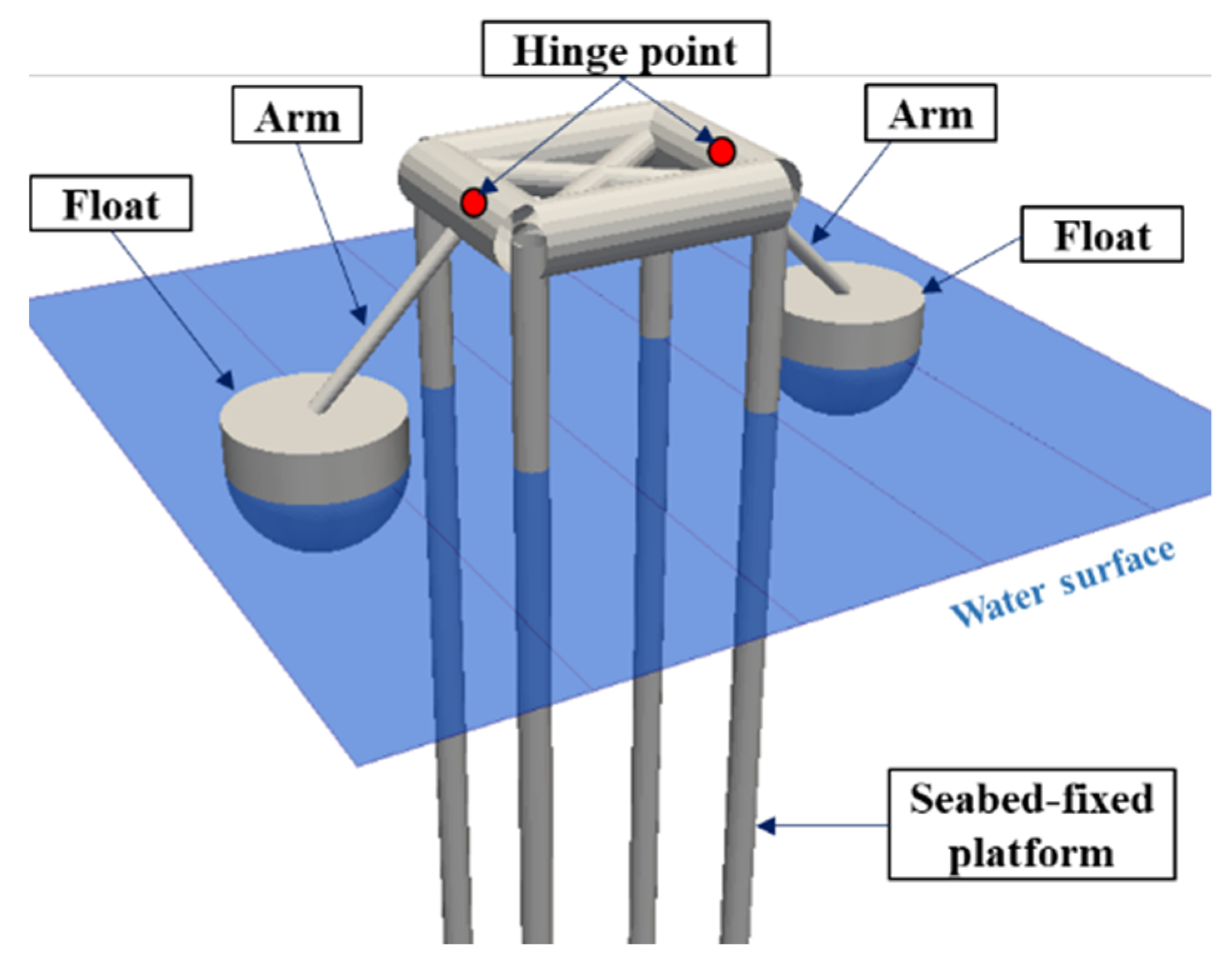
Wavestar is an oscillating body heaving-point-absorber (HPA) WEC [8]. Figure 1 shows a Wavestar-type WEC platform model applied in this study. It is composed of multiple hemispherical floats and a seabed-fixed platform. Each float is connected to a hinge point on the platform with an arm, and its heave motion is converted to rotational motion [4]. External forces, including incident wave loads, act on the floats. Each float moves up and down and generates electricity using the PTO system. In the case of a multiple-floating-body system, the hydrodynamic interactions between the floats should be considered [9]. Many studies have evaluated the motion of the float and the power production of Wavestar-type WECs. Zurkinden et al. [10] conducted an experimental study and numerical analysis for a single float in a Wavestar WEC. They reported that the linear assumption of the external moments was in good agreement with the physical model. Kim et al. [11] carried out an experimental study for the motion characteristics of a hinged floating WEC. They examined the hydrodynamic responses and the generated power of a hemispherical float. Wang et al. [12] developed a flexible multibody dynamics model for hinged-point-absorber WECs. They analyzed the floater arm tip displacement and velocity, as well as the stress distribution of an arm. Heo and Koo [13] performed a linear time-domain analysis of a Wavestar-type WEC using the multibody dynamics formulation in the two-dimensional domain. They compared the time history results with the classical method and reported results that were in good agreement with each other. Ghafari et al. [14] presented a hybrid platform that combined a floating wind turbine and multiple Wavestar-type WECs. They evaluated both the motion of the floating platform and power production according to various environmental conditions and the number of floats.

The Korean government announced the Renewable Energy 3020 plan, which aims to increase the proportion of renewable energy generation to 20% of the total generation output by 2030 [15,16]. The Korean peninsula is surrounded by sea on three sides (East Sea, South Sea, and Yellow Sea) and is suitable for applying the WEC [17]. Several researchers have reviewed the offshore and nearshore wave energy resources for the region around the Korean peninsula [18,19,20]. Ahn and Ha [21] assessed and characterized the wave energy resources using wave measurements at 22 buoy stations around Korea. They calculated and compared the total wave power, peak period spread, and monthly variability to determine the ideal areas in terms of wave energy resources in the nearshore areas of Korea. Research on WECs, applying the environmental conditions of the Korean nearshore, is being actively conducted. Kim and Koo [22] performed time-domain analysis to determine the optimal design of a two-buoy-type WEC, applying three-year measured wave data from Uljin, Korea. Ko et al. [23] carried out numerical analysis and an experimental study to investigate the optimal PTO torque of an asymmetric WEC under the wave conditions of the western sea of Jeju Island, Korea. Kim et al. [24] proposed a dual-buoy WEC that generates electricity using the relative motion between two buoys. They analyzed the dynamic characteristics of the WEC using actual wave data measured at two sites in Hupo Harbor, Korea.

In this study, the numerical procedure developed in the authors’ previous study (Heo and Koo, 2020) was extended to a three-dimensional model. In addition, the nonlinear Froude–Krylov force was used to calculate the nonlinear body force in waves. A spherical float was used as a WEC model, and the waterplane area of the float was changed in time, so the time-varying nonlinear Froude–Krylov force was updated in every time step to reflect the nonlinear effect. In the previous study [13], for the analysis of the heaving-point-absorber WEC, an augmented formulation, one of the multibody dynamics techniques, was developed and applied to construct an equation of motion for a two-dimensional plane, and only a linear time-domain analysis was performed. Frequency-dependent hydrodynamic coefficients of a single float and two floats were obtained using the the boundary element method (BEM)-based hydrodynamic solver WAMIT [25]. Time-domain simulation was carried out, applying the linear and weakly nonlinear hydrodynamic analysis methods for the floating body. For the 3D WEC model applied in this study, four nearshore areas in Korea were selected. To compare the trends and magnitudes of the results, regular waves were applied as the environmental conditions. The regular wave conditions were calculated using six-year average winter wave data obtained from the Korea Meteorological Administration (KMA) and used for numerical analysis. The dynamic responses and power production of the Wavestar-type WECs were analyzed for the selected areas.

2. Calculation Methods

2.1. Equation of Motion of a Constrained Rigid Body System

The equation of motion of a constrained rigid body system can be expressed as a differential equation using Newton’s second law and an equation expressing the constraint conditions between objects as algebraic equations [26].

$$M\ddot{u}=Q-C_u^T\lambda$$

(1)

$$C\left(u,t\right)=0$$

(2)

where $M$, $u$, $Q$, $C$, $C_u$, and $\lambda$ are the mass matrix, displacement vector, generalized external force vector, constraint equation vector of the system at the displacement level, the Jacobian matrix of constraint equations $\left(C_u=\partial C/\partial u\right)$, and the Lagrange multiplier vector, respectively. Euler angles were used to transform the body-fixed frame to an earth-fixed frame [27]. The second term on the right-hand side of Equation (1) represents the constraint force acting on the center of gravity of each object caused by the constraint condition. The first and second derivatives with respect to time of Equation (2) were obtained to determine the constraint equations at the velocity and acceleration levels, respectively.

$$C_u\dot{u}=-C_t$$

(3)

$$C_u\ddot{u}=Q_d=-\left({\left(C_u\dot{u}\right)}_u\dot{u}+2C_{ut}\dot{u}+C_{tt}\right)$$

(4)

The dynamic response of the constrained system can be obtained via the numerical analysis of the differential-algebraic equations composed of Equations (3) and (4). Equation (5) shows the equation of motion using the augmented formulation, one of the multibody dynamics formulations [28].

$$\left[\begin{array}{cc}M& C_u^T\\ C_u& 0\end{array}\right]\left\{\begin{array}{l}\ddot{u}\\ \lambda \end{array}\right\}=\left\{\begin{array}{c}Q\\ Q_d\end{array}\right\}$$

(5)

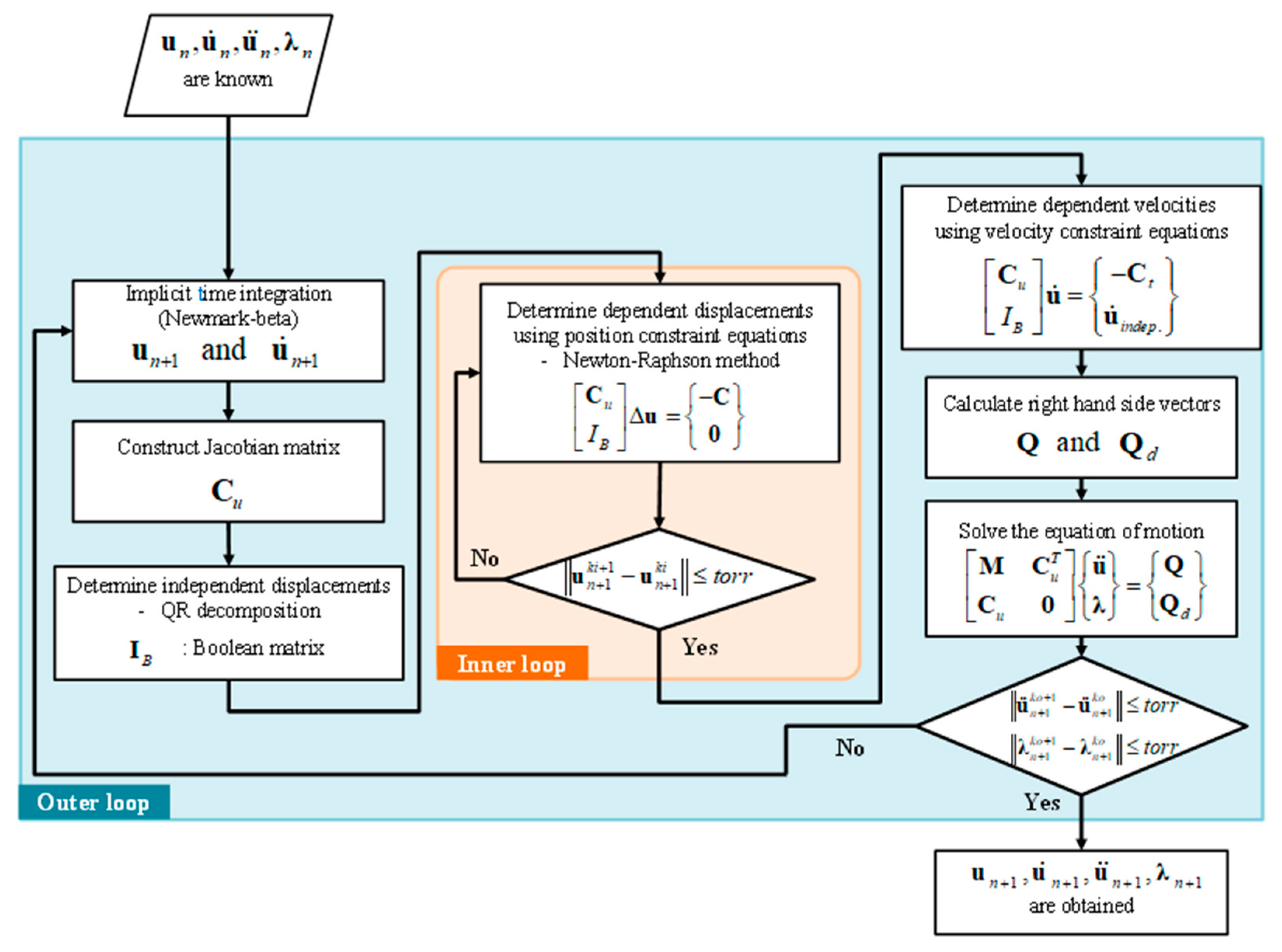
Equations (2)–(4) cannot be satisfied accurately because of an error occurring in the numerical integration process of Equation (5) [29]. To solve this problem, time integration was performed using a two-loop procedure to ensure that the errors of the constraint equations at displacement, velocity, and acceleration levels were within the tolerance [26,29,30].

Figure 2 shows the two-loop procedure for the implicit time-integration method. First, the n^th time step variables enter the outer loop. The displacement and velocity were obtained at the next time step, using the implicit time integration scheme. Subsequently, the Jacobian matrix was constructed, and the independent displacements were determined. The dependent displacements were calculated by applying the Newton–Raphson method to the displacement constraint equations, in a process called an inner loop. The dependent velocities were calculated using the velocity constraint equation. Finally, the right-hand side of the equation of motion was calculated, and the motion equation was solved to obtain the (n+1)^th time step’s variables.

2.2. External Forces Acting on the Floating Body

Various external forces acting on the floating body can be expressed as follows:

$${\displaystyle \sum F}=F_{Weight}+F_{Hydrostatic}+F_{Froude–Krylov}+F_{Diffraction}+F_{Radiation}$$

(6)

where $F_{Weight}$ is the self-weight, $F_{Hydrostatic}$ is the hydrostatic force, $F_{Froude–Krylov}$ is the Froude–Krylov force, $F_{Diffraction}$ is the diffraction force, and $F_{Radiation}$ is the wave radiation force.

The self-weight acts in the vertical downward direction and is calculated as the product of the mass of the body ($m$) and the gravitational acceleration ($g$) as follows:

$$F_{Weight}={\left[\begin{array}{ccc}0& 0& -mg\end{array}\right]}^T$$

(7)

The hydrostatic force can be calculated using linear or nonlinear analysis. The linear hydrostatic force is obtained through an equation that is linearly proportional to the submerged depth of the body from the still water level regardless of the change in the water surface with time. On the other hand, the nonlinear hydrostatic force can be obtained by integrating the pressure acting on the submerged area at every time step. Equations (8) and (9) represent the linear and nonlinear hydrostatic force, respectively.

$$F_{Hydrostatic\_Linear}={\left[\begin{array}{ccc}0& 0& {\rho }_{w}g\left(V_s-A_w{u}_z(t)\right)\end{array}\right]}^T$$

(8)

$$F_{Hydrostatic\_Nonlinear}\left(t\right)=-{\displaystyle {\iint }_{S_B(t)}{\rho }_{w}g{u}_z\hspace{0.17em}n}\hspace{0.17em}dS$$

(9)

where ${\rho }_w$, $V_s$, $A_w$, $u_z$, $S_B$, $n$, and $dS$ are the density of seawater, the volume of displacement of the body in calm water, the waterplane area of the body, the vertical displacement of the body from the still water level, the submerged surface, the normal vector of the infinitesimal area, and the infinitesimal area, respectively.

The Froude–Krylov and diffraction forces can also be obtained through linear or nonlinear analysis. The linear Froude–Krylov and diffraction forces can be calculated through frequency-domain analysis using the boundary element method. In this study, the frequency-dependent Froude–Krylov and diffraction forces were computed using the hydrodynamic solver WAMIT [25].

$$F_{Froude–Krylov\_Linear}\left(t\right)=\frac{{\rho }_{w}gH}{2}\cdot \left|F_{FK}\left(\omega \right)\right|\cdot \cos \left(k\cdot \left(x\cos \alpha +y\sin \alpha \right)-\omega t\right)$$

(10)

$$F_{Diff}\left(t\right)=\frac{{\rho }_{w}gH}{2}\cdot \left|F_{Diff}\left(\omega \right)\right|\cdot \cos \left(k\cdot \left(x\cos \alpha +y\sin \alpha \right)-\omega t\right)$$

(11)

where $H$ is the wave height. $\left|F_{FK}\left(\omega \right)\right|$ and $\left|F_{Diff}\left(\omega \right)\right|$ are the magnitude of the Froude-Krylov and diffraction forces calculated using WAMIT, respectively. $k$ is the wavenumber. $\alpha$ is the incident wave direction, and $\omega$ is the incident wave frequency.

The nonlinear Froude–Krylov (FK) force should be considered when performing analysis on HPA type WECs [31]. The nonlinear FK force can be obtained by integrating the dynamic pressure acting on the submerged surface of the body at every time step as follows [32]:

$$F_{Froude–Krylov\_nonlinear}=-{\displaystyle {\iint }_{S_B(t)}{\rho }_w{p}_{FK}n}\hspace{0.17em}dS$$

(12)

$$p_{FK}=\frac{{\rho }_{w}gH}{2}\frac{\cosh \left(kz\right)}{\cosh \left(kh\right)}\cos \left(k\left(x\cos \alpha +y\sin \alpha \right)-\omega t\right)$$

(13)

where $p_{FK}$ is the dynamic pressure acting on the submerged surface of the body.

The wave radiation force can be obtained using Cummins’ equation, considering the time memory effect. The equation is expressed through the convolution integral between the retardation function and the velocity of the body [33,34]. The wave radiation force in direction $l$ can be expressed as

$$F_{Radiation,l}\left(t\right)=-m_{a_{\infty },lm}\left(\omega \right)\cdot {\ddot{u}}_m\left(t\right)-{\displaystyle {\int }_0^t{K}_{lm}\left(\tau \right)·{\dot{u}}_m\left(t-\tau \right)d\tau }$$

(14)

where $m_{a_{\infty }}$ is the added mass at infinite frequency. $K$ is the retardation function, as follows [35]:

$$K_{lm}\left(t\right)=\frac{2}{\pi }{\displaystyle {\int }_0^{\infty }{b}_{lm}\left(\omega \right)\cdot \cos \left(\omega t\right)d\omega }$$

(15)

where $b$ is the radiation damping coefficient calculated using WAMIT [25].

Table 1. Hydrodynamic analysis methods for the floating body.

Force	Linear Analysis	Weakly Nonlinear Analysis	Fully Nonlinear Analysis
Froude–Krylov	Linear	Nonlinear	Nonlinear
Hydrostatic	Linear	Nonlinear	Nonlinear
Diffraction	Linear	Linear	Nonlinear
Radiation	Linear	Linear	Nonlinear

lists the hydrodynamic analysis methods for the floating body. In this study, linear and weakly nonlinear analyses were considered.

When multiple floats are placed, the motion of each float affects the surrounding flow field, which in turn influences the motion of the surrounding floats. In this study, the hydrodynamic coefficients with the two-body interaction were obtained using the BEM-based frequency-domain hydrodynamic solver WAMIT. The equation of the motion of the floats, considering the hydrodynamic interaction, can be expressed in terms of complex amplitude as follows [25,36]:

$$\left[-{\omega }^2\left(m^p+m_a^{p,p}\right)+i\omega b^{p,p}+c^p\right]{\xi }^p+{\displaystyle \sum _{\begin{array}{c}q=1\\ q\ne p\end{array}}^P\left[-{\omega }^2{m}_a^{p,q}+i\omega b^{p,q}\right]{\xi }^q}=X^p$$

(16)

where $m$ denotes the mass matrix of the float. Matrices $m_a$ and $b$ denote the frequency-dependent added mass and radiation damping coefficient matrix, respectively. $c$ denotes the hydrostatic coefficient matrix. Vectors $\xi$ and $X$ denote the complex amplitude of the motion of the float and excitation force vector, respectively. $p$ and $q$ denote the $p$-th and $q$-th floating body, respectively. $P$ denotes the number of floating bodies.

The interaction between the floating bodies affects not only the external force but also the motion characteristics of the bodies. In this study, numerical analysis of two floats was performed using frequency-dependent coefficients with the two-body hydrodynamic interaction.

3. Numerical Simulation

3.1. Verification of Numerical Results

3.1.1. Heave Motion of a Single Spherical Float

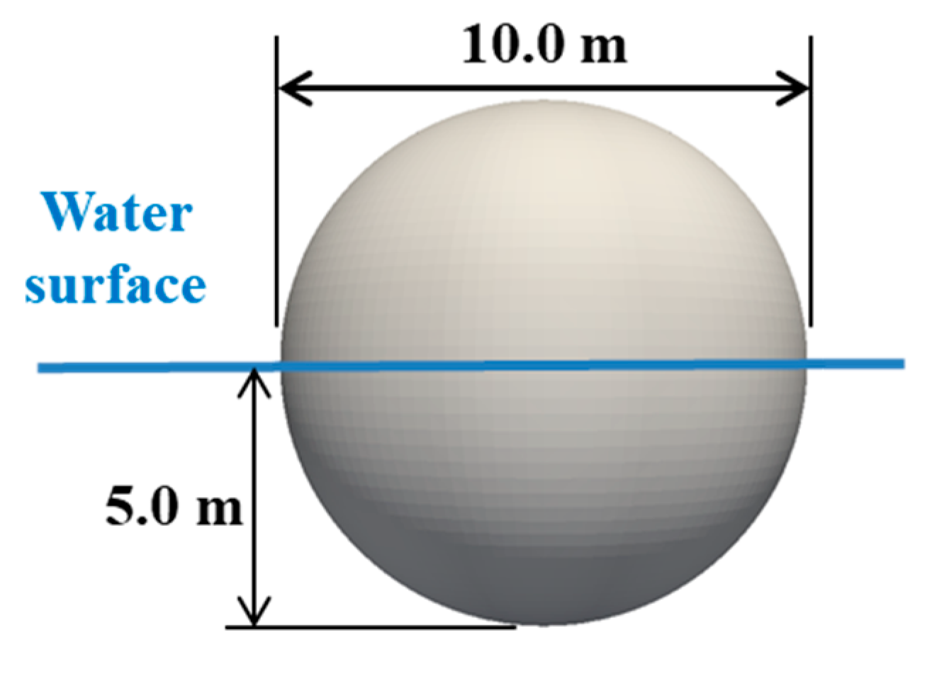
Figure 3 depicts a spherical float with a 10-m diameter. The draft was 5 m, and the mass was 261,800 kg. An infinite-depth condition was applied, and the density of the water was 1000 ${\mathrm{kg}/\mathrm{m}}^3$. This model was composed of 7200 quadrilateral elements.

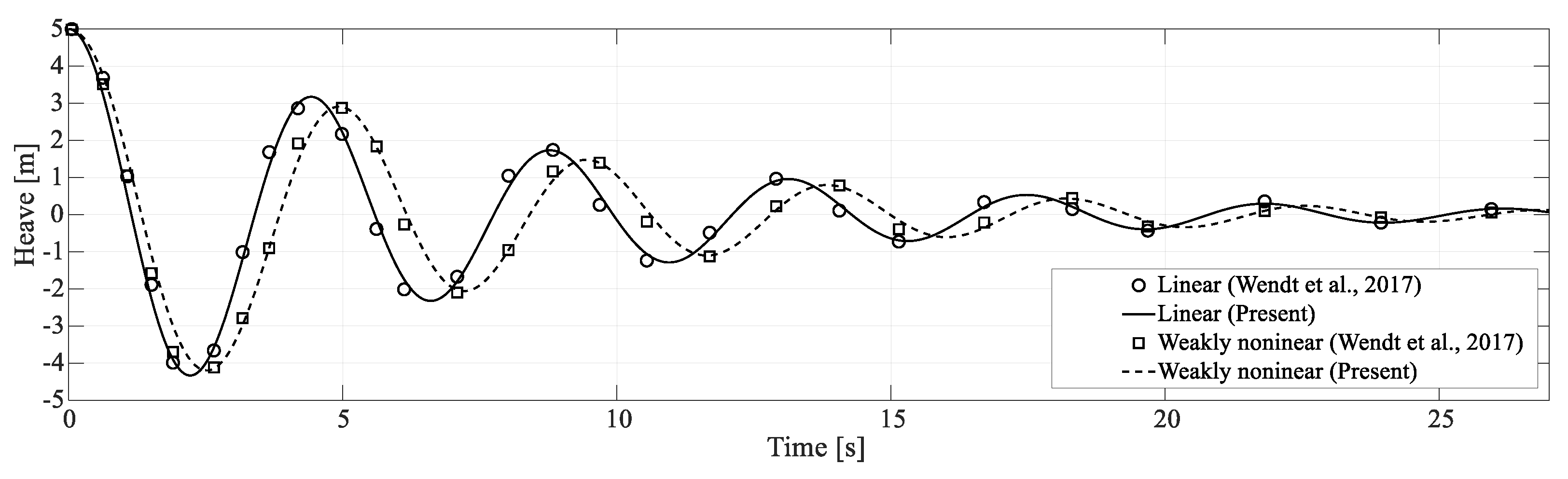
Figure 4 compares the results of the linear and weakly nonlinear analysis for the heave free-decay test with the reference literature when the initial position was 5 m above the water surface [37]. The results agree well. The time series of the linear and weakly nonlinear analysis have different magnitudes and phase angles because the difference between the nonlinear and linear hydrostatic force caused by the geometric nonlinearity of the sphere was large.

The heave response amplitude operator (RAO) under regular wave conditions in the time domain can be calculated by dividing half of the peak (crest)-to-trough oscillation by the wave amplitude.

$$RA{O}_{Heave}=\frac{\left(z_{\max }-z_{\min }\right)}{2}\cdot \frac{1}{A}=\frac{\left(z_{\max }-z_{\min }\right)}{H}$$

(17)

where $z_{\max }$ and $z_{\min }$ denote the maximum (crest) and minimum (trough) heave time series, respectively. $A$ denotes the wave amplitude. The following PTO damping force was also applied to the external force vector of the float to evaluate the heave RAO with PTO damping [37].

$$F_{PTO}={\left[\begin{array}{ccc}0& 0& -B_{PTO}\cdot \dot{z}\end{array}\right]}^T$$

(18)

$$B_{PTO}=b_{33}\left(\omega \right)\cdot \sqrt{1+{\left(\frac{{\rho }_{w}g{A}_w-{\omega }^2\cdot \left(m+m_a\left(\omega \right)\right)}{\omega \cdot b_{33}\left(\omega \right)}\right)}^2}$$

(19)

where $B_{PTO}$ is the PTO damping coefficient.

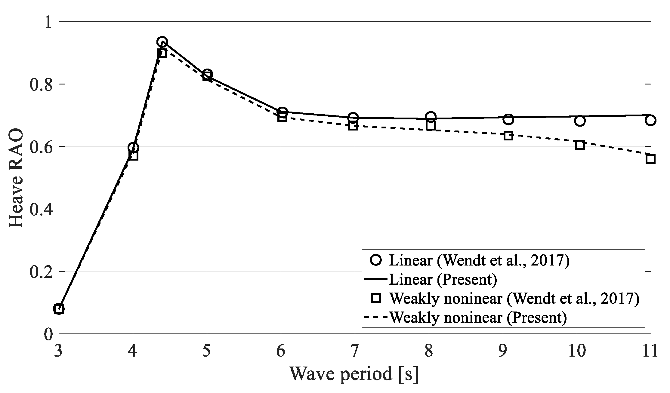
Figure 5 compares the heave RAO of the float with PTO damping with the reference literature when the wave steepness was constant at 0.0628. The magnitude and trend showed good agreement. When the wave period was greater than seven seconds, the heave of the floating body was affected more when the weakly nonlinear analysis was considered, compared to the linear analysis.

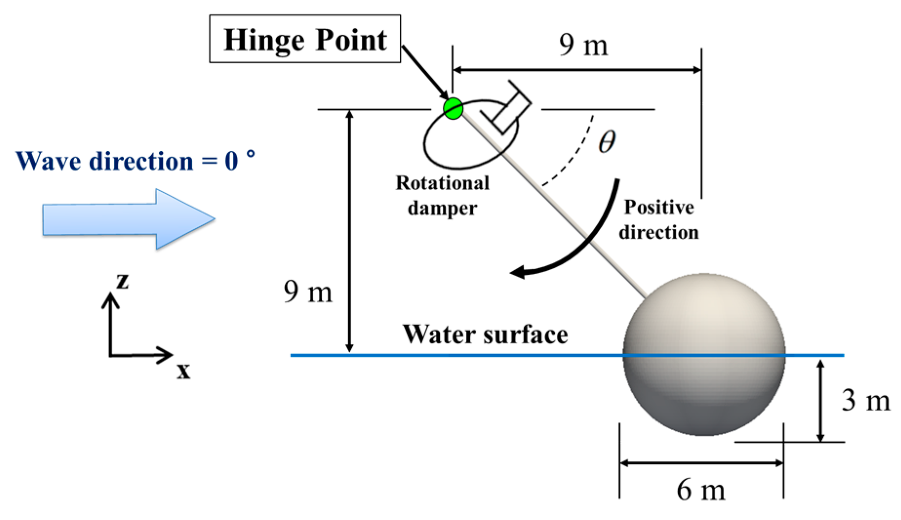
3.1.2. Motion of a Spherical Float Constrained to a Hinge Point

Figure 6 presents a spherical float constrained to a hinge point. The diameter and draft of the float were 6 m and 3 m, respectively. The mass of the float and water depth were 57,962 kg and 20 m, respectively. This float could only rotate in the y-axis because of the hinge joint. The rotational damper was applied to describe the PTO extraction (damping) system. The moment acting on the hinge point due to the PTO system can be expressed as

$$M_{PTO}\left(t\right)=B_{PTO,rot}\cdot \dot{\theta }\left(t\right)$$

(20)

where $\dot{\theta }$ is the angular velocity of the float and $B_{PTO,rot}$ is the rotational PTO extraction coefficient for the available wave power. For the comparison, the $B_{PTO,rot}$ of $3.52\times {10}^6$ $N·m·s$ was used.

The pitch RAO of the float under regular wave conditions in the time domain can be computed similarly to Equation (17) as follows:

$$RA{O}_{Pitch}=\frac{\left({\theta }_{\max }-{\theta }_{\min }\right)}{H}$$

(21)

where ${\theta }_{\max }$ and ${\theta }_{\min }$ denote the maximum and minimum rotation angles, respectively.

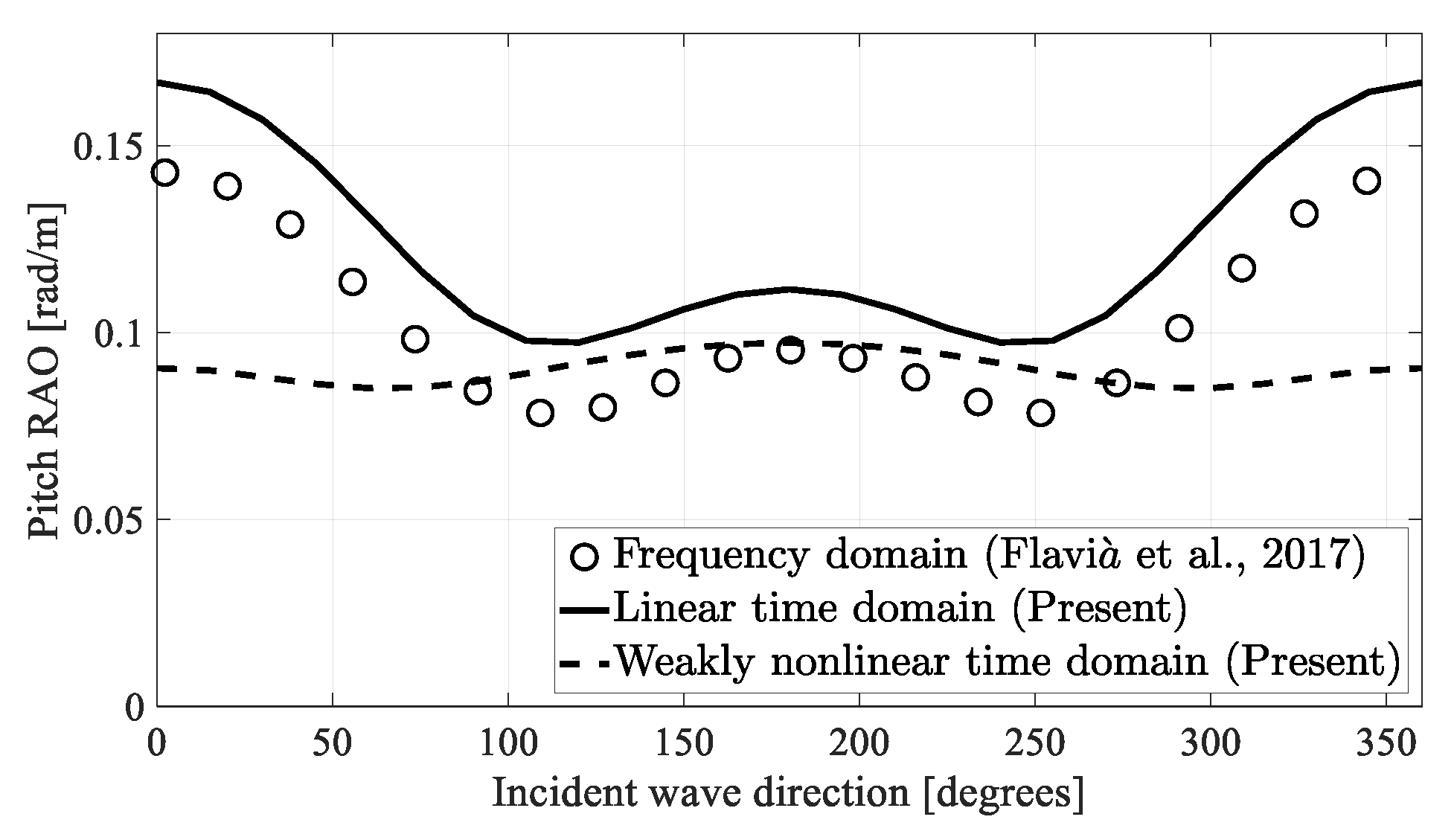
Figure 7 compares the pitch RAO of the float according to the incident wave direction obtained through linear and weakly nonlinear time-domain analysis with the frequency domain results from the literature [38]. A wave height of 2 m and a wave frequency of 1.4 rad/s were applied. The pitch RAO from the linear time-domain analysis and from the reference results showed similar trends. However, the magnitudes of the pitch RAO of the linear analysis were consistently larger than those of the reference. This is because the added mass, radiation damping, and hydrostatic stiffness used in the frequency-domain analysis of the reference were not the same values as the coefficients used in the linear time-domain analysis of this study. The hydrostatic stiffness for the rotation axis was calculated by considering both the roll stiffness and the heave stiffness. On the other hand, in this study, since a spherical buoy was applied, the hydrostatic stiffness for the rotation axis was obtained by considering only the heave stiffness and ignoring the effect of the roll stiffness. The heave hydrostatic force of the float was converted into a moment acting on the hinge point via the constraint condition. Therefore, the difference in pitch RAO is due to the difference in the calculation process and the coefficients used. Nevertheless, the comparative analysis is meaningful because the two linear calculation results have the same overall tendency according to the angle of the incident wave.

The weakly nonlinear time-domain results showed a different trend and magnitude from the linear analysis results. This is due to the different phase angles of the diffraction force depending on the position of the float and the influence of nonlinear Froude–Krylov forces.

3.2. Simulation Results and Analysis

3.2.1. Single Hemispherical Float

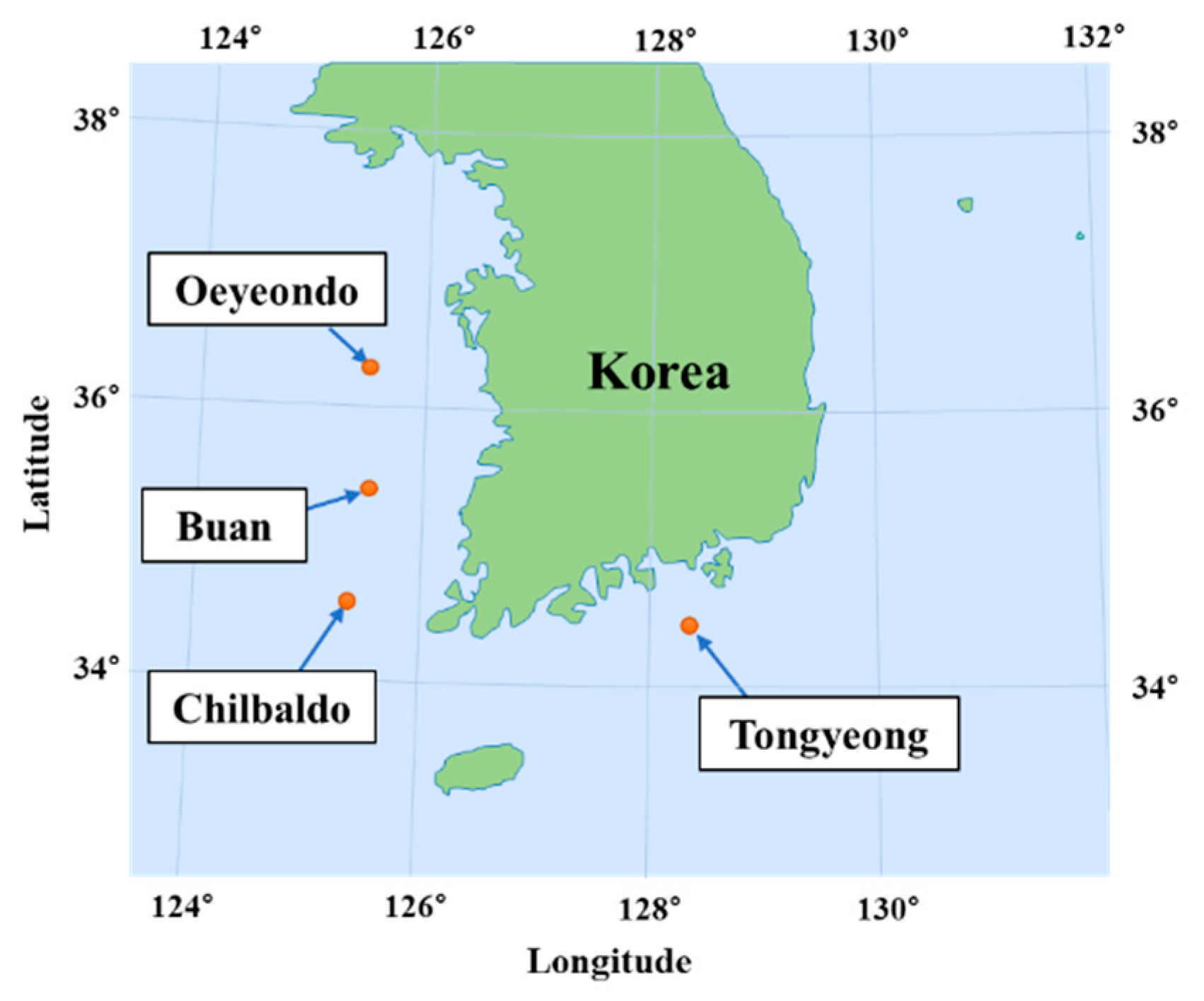
The fixed-platform Wavestar-type WEC should be installed in an area where the water depth is shallow and the potential wave force is large. In this study, four nearshore regions of wave buoys in Korea with suitable environmental conditions were selected to install the fixed-platform Wavestar WEC [21]. Figure 8 shows the location of the four wave buoys selected for wave data measurements, i.e., Chilbaldo, Oeyeondo, Buan, and Tongyeong. The six-year average winter wave data were obtained from KMA (from November to February during the period from 2015/2016 to 2020/2021) [39]. Using the collected wave data, the regular wave conditions was calculated and applied to the numerical analysis to compare the dynamic responses and energy extraction performance of a Wavestar-type WEC according to each environmental condition in Korean nearshore areas.

Table 2. Regular wave conditions calculated from buoy data in each selected area.

Buoy	Location		Water Depth (m)	Wave Height (m)	Wave Period (s)	Wave Steepness	Incident Wave Power (kW/m)
	Latitude	Longitude
Chilbaldo	34°47′36″ N	125°46′37″ E	33	1.26	5.46	0.0273	8.508
Oeyeondo	36°15′00″ N	125°45′00″ E	47	1.23	5.43	0.0265	8.059
Buan	35°39′31″ N	125°48′50″ E	50	1.28	5.46	0.0275	8.764
Tongyeong	34°23′30″ N	128°13′30″ E	55	1.24	5.38	0.0275	8.108

lists the geographic and ocean environmental conditions for each buoy. Linear (Airy) wave theory was used to describe the water particle kinematics. The incident wave power per unit crest width of a regular wave can be expressed as follows [40]:

$$P_{Wave}=\frac{1}{8}{\rho }_{w}g{H}^2{C}_g$$

(22)

where $C_g$ is the group velocity. A water density of 1025 ${\mathrm{kg}/\mathrm{m}}^3$ was applied for all simulation cases. Among the four locations, Buan exhibited the largest incident wave power. This was attributed to the deep water, large wave height, and long wave period compared to the other locations.

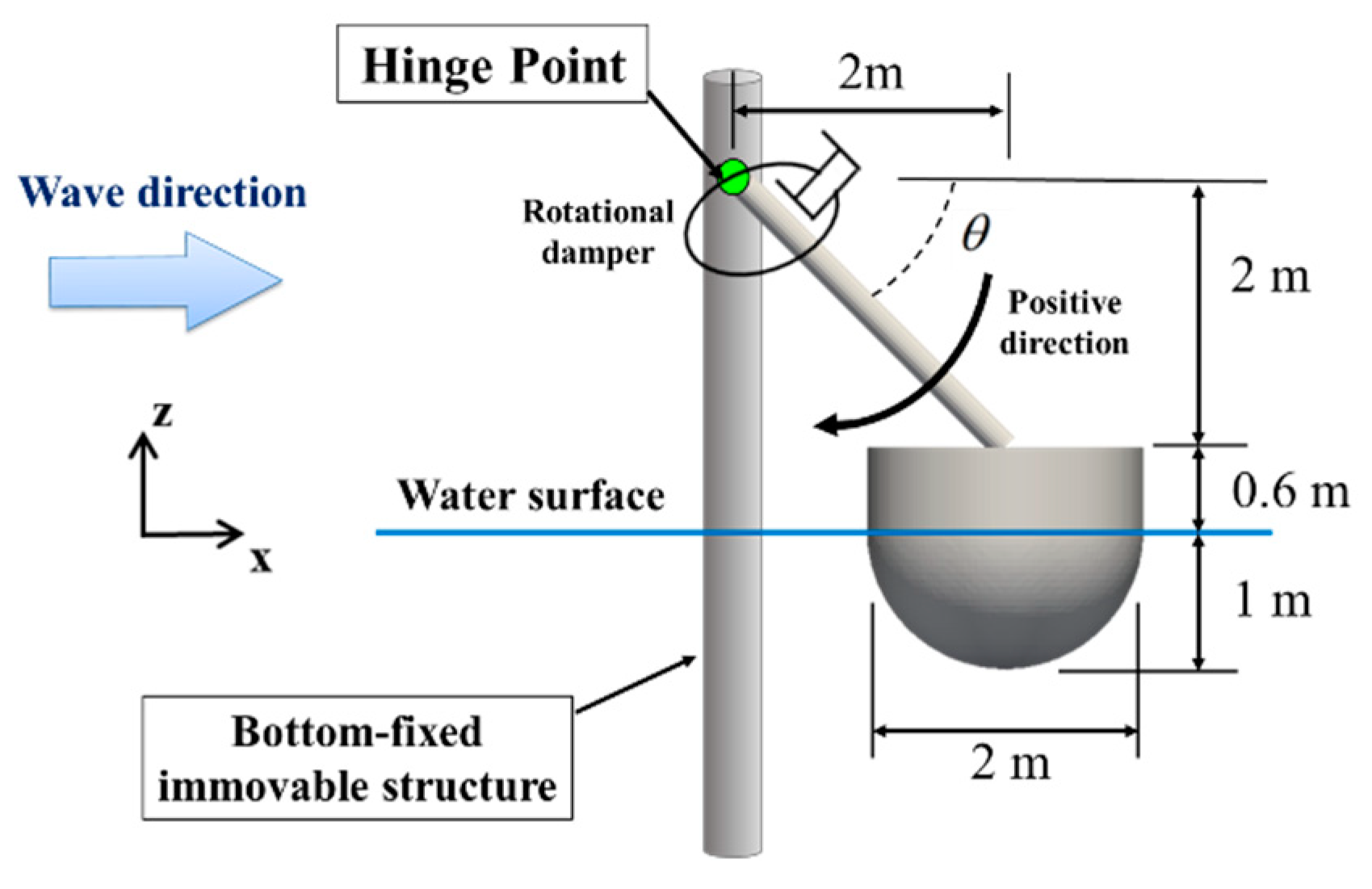
Figure 9 presents a single floating body HPA-type WEC with a hemispherical shape below the water surface. The diameter and draft of the float were 2 m and 1 m, respectively. The mass of the float was 2147 kg. The upper part of the float has a cylindrical shape with the same diameter as the hemisphere. This model was composed of 8520 quadrilateral elements. The float was assumed to be connected by a massless rigid arm to a hinge point on a bottom-fixed column structure that had a much smaller column diameter than the incident wavelength and which did not generate any scattered waves. The float will only have rotational motion in the y-axis direction due to the hinge joint. Rotational damping is applied to the hinge point to describe the PTO system. The power produced by the PTO system can be evaluated using the following equation [14].

$$P_{PTO}\left(t\right)=B_{PTO,rot}\cdot {\left\{\dot{\theta }\left(t\right)\right\}}^2$$

(23)

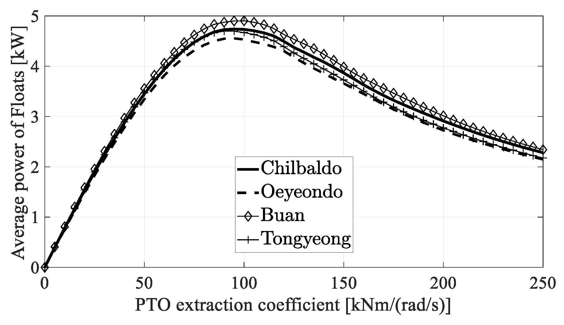
The motion of the float and the power production depend on the PTO extraction coefficient. The optimal PTO extraction coefficient was determined by evaluating the average powers for various extraction coefficients at four locations under the environmental conditions in Table 2. Figure 10 shows the average power production of the float according to the extraction coefficient of the PTO system. The average wave power output showed the largest value in Buan regardless of the PTO extraction coefficient. This is because its incident wave power was larger than that in the other locations. The optimal PTO extraction coefficients at each location shown in

Table 3. Optimal extraction coefficients at each location.

Location	Optimal Extraction Coefficient (kN$·$m/(rad/s))
Chilbaldo	95.0
Oeyeondo	95.0
Buan	100.0
Tongyeong	90.0

were applied for all subsequent calculations.

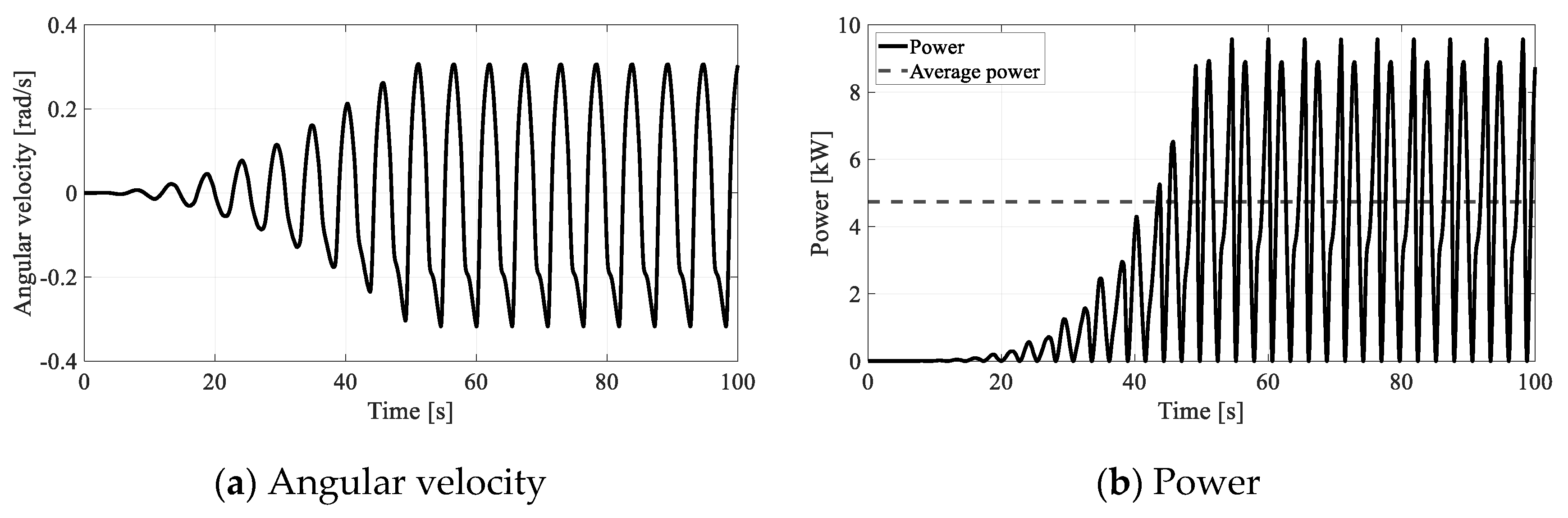
Figure 11 shows the time history of the angular velocity and power of the single float at Chilbaldo from 0 to 100 s. The optimal extraction coefficient of 95.0 kN$·$m/(rad/s) at Chilbaldo was applied. The angular velocity of the float ranged from −0.3174 to 0.3061 rad/s. As shown in Figure 9, the positive rotation direction is the direction in which the float descends. Therefore, a larger negative value of the angular velocity means that the velocity of the float is greater as it rises. In other words, the float produces more power as it rises.

As shown in Figure 11b, the power production changed according to the rotation direction of the float. At Chilbaldo, the average power production was approximately 4.74 kW, and the peak power occurred when the float ascended and was approximately 9.57 kW.

Table 4. Average power, CWR, and peak power at each location.

Location	Average Power (kW)	CWR	Maximum Power (kW)
Chilbaldo	4.738	0.278	9.572
Oeyeondo	4.554	0.283	9.077
Buan	4.900	0.280	9.959
Tongyeong	4.697	0.290	9.382

lists the average power, capture width ratio (CWR), and peak power at each location. The average power at Buan was larger than in other locations. This was attributed to the relatively large incident wave power, as mentioned above. To compare the power productions, CWR was calculated as [14]

$$CWR=\frac{P_{PTO,avg}[kW]}{D[m]\cdot P_{Wave}[kW/m]}$$

(24)

where $P_{PTO,avg}$ is the average power production and $D$ is the diameter of the float. Unlike the power production, the CWR was the largest at Tongyeong. This means that Tongyeong showed the best efficiency in terms of wave power production.

3.2.2. Two Hemispherical Floats

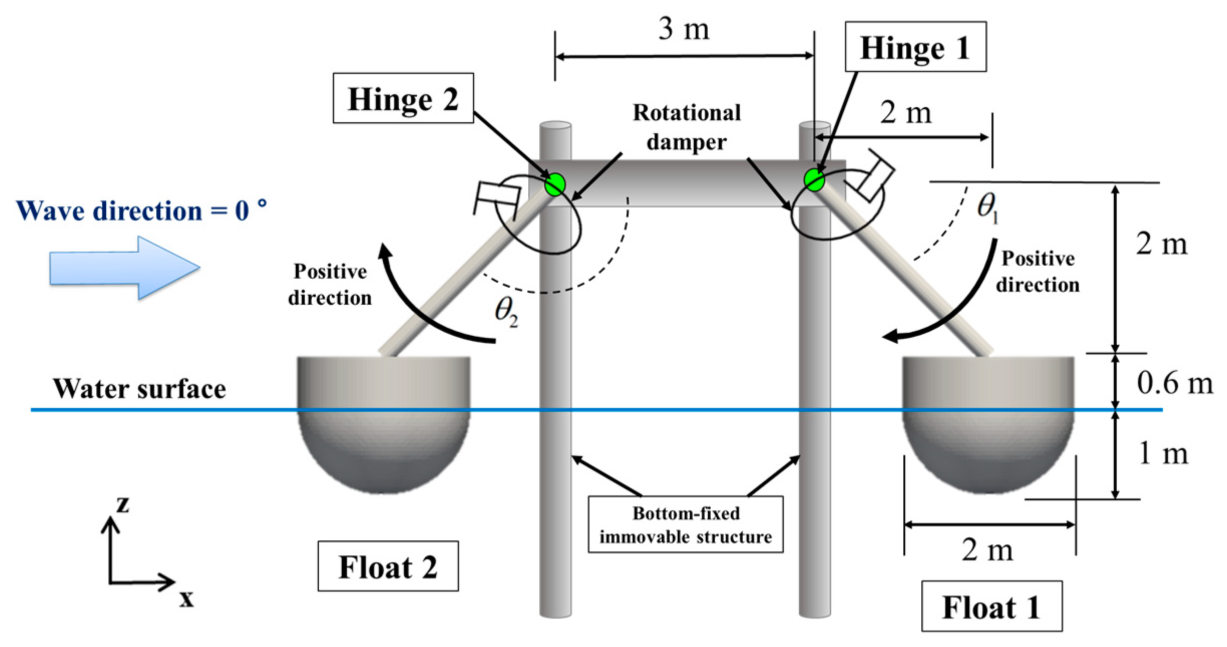
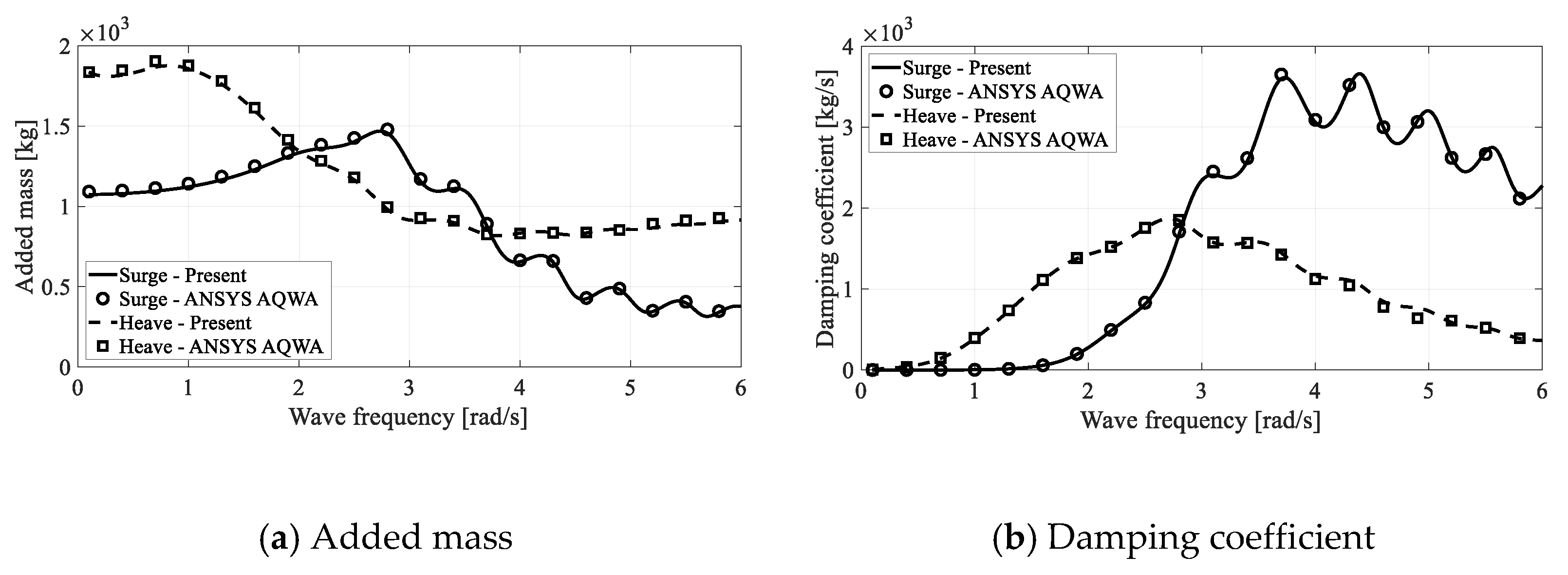
Figure 12 presents a two-buoy HPA-type WEC model with two floats. Because the vertical pile is a slender cylinder, there is no scattered wave effect. Therefore, it is assumed that there is no interaction between the pile and float. The distance between the two hinge points was 3 m. Float 1 and Float 2 have the same hydrodynamic coefficients because they have the same shape and size. Figure 13 compares the added mass and radiation damping coefficients of the float used in this study with the results of the hydrodynamic solver ANSYS AQWA [25,41]. The results were in good agreement with each other. Since these coefficients are influenced by the hydrodynamic interactions between the floats, it is essential to take them into account. In the Wavestar-type platform, the surge motion has a significant effect on the rotational motion of the floats.

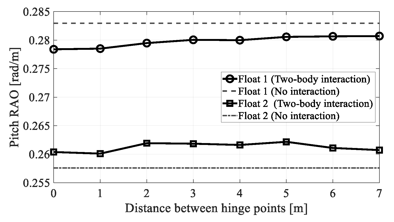
Figure 14 compares the pitch RAO of the float at Chibaldo according to the distance between the hinge points. As distance increases, the pitch RAO with two-body interaction tends to approximate the results of a single float (no interaction). However, the difference is very small, less than 1%. This is because the float diameter is very small compared to the wavelength, so the effect of the diffracted wave generated from the float is small.

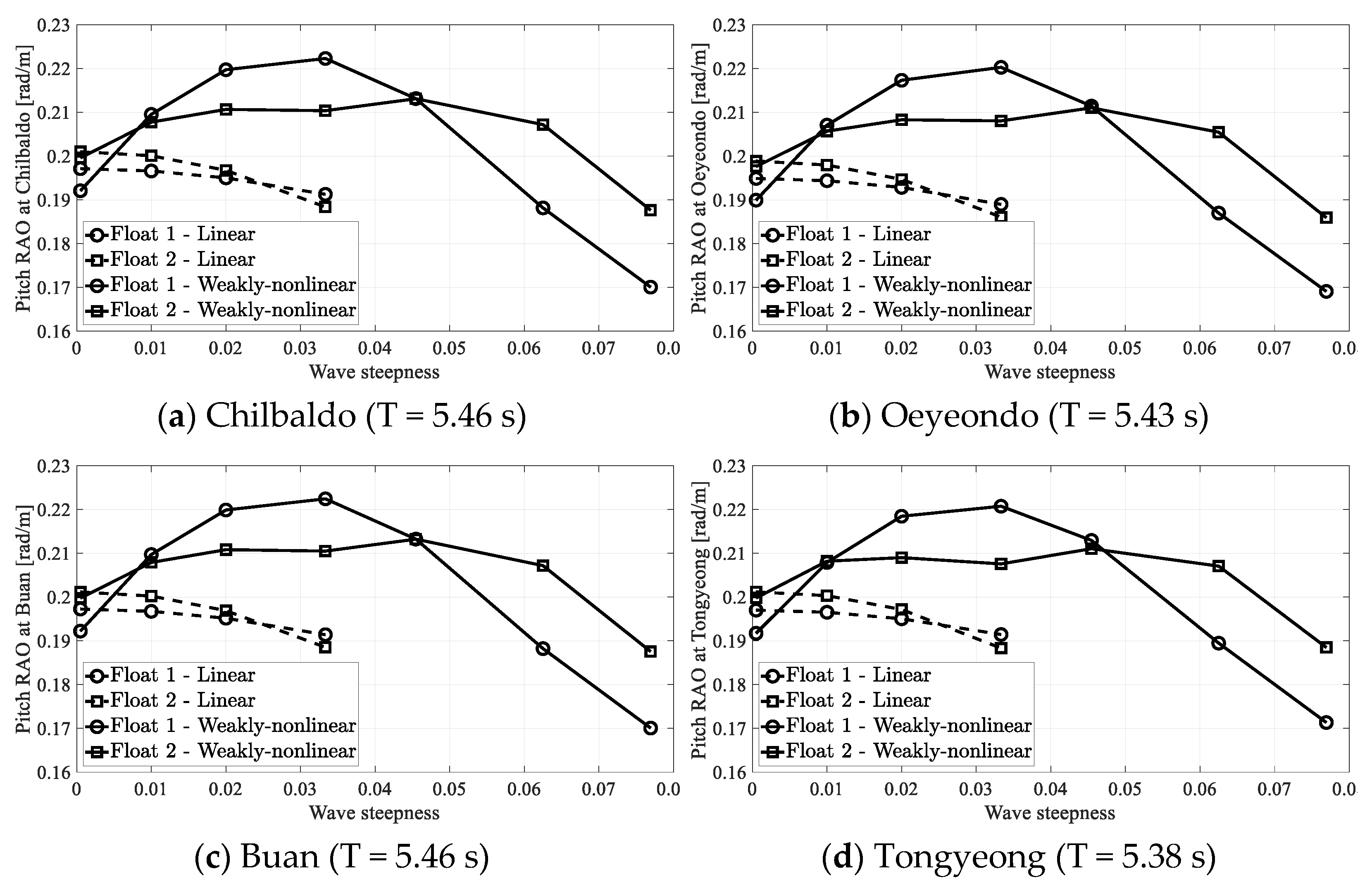
First, when the wave period has a constant value for each location, the effects of a change in the wave height were compared. Figure 15 represents the pitch RAO assessed through linear and weakly nonlinear analysis according to the wave steepness when a wave with the period shown in Table 2 acts on each location. In the case of linear analysis, when the wave steepness was greater than 0.0455 (1/22), the results were inaccurate and were excluded from the comparison. The result for each location was generally similar in magnitude and trend regardless of the location because the environmental conditions were similar. The linear and weakly nonlinear analysis results showed a difference of approximately 5 % when the wave steepness was close to zero. On the other hand, the difference in the magnitude and trend of pitch RAO between the two methods increased significantly as the incident wave steepness increased. This means that time-domain analysis considering the nonlinear components of the external force must be performed for the design of Wavester-type WEC. The magnitude of the pitch RAO of the float varies with the wave steepness, which can be attributed to the change in the magnitude of the moment acting on the center of rotation of the float. When the wave steepness was between 0.02 (1/50) and 0.0455, the pitch RAO of Float 1 (rear body) was greater than that of Float 2 (front body). Because the wave steepness shown in Table 2 falls within this range, it can be expected that power production will be larger for Float 1 (rear body) in real sea conditions.

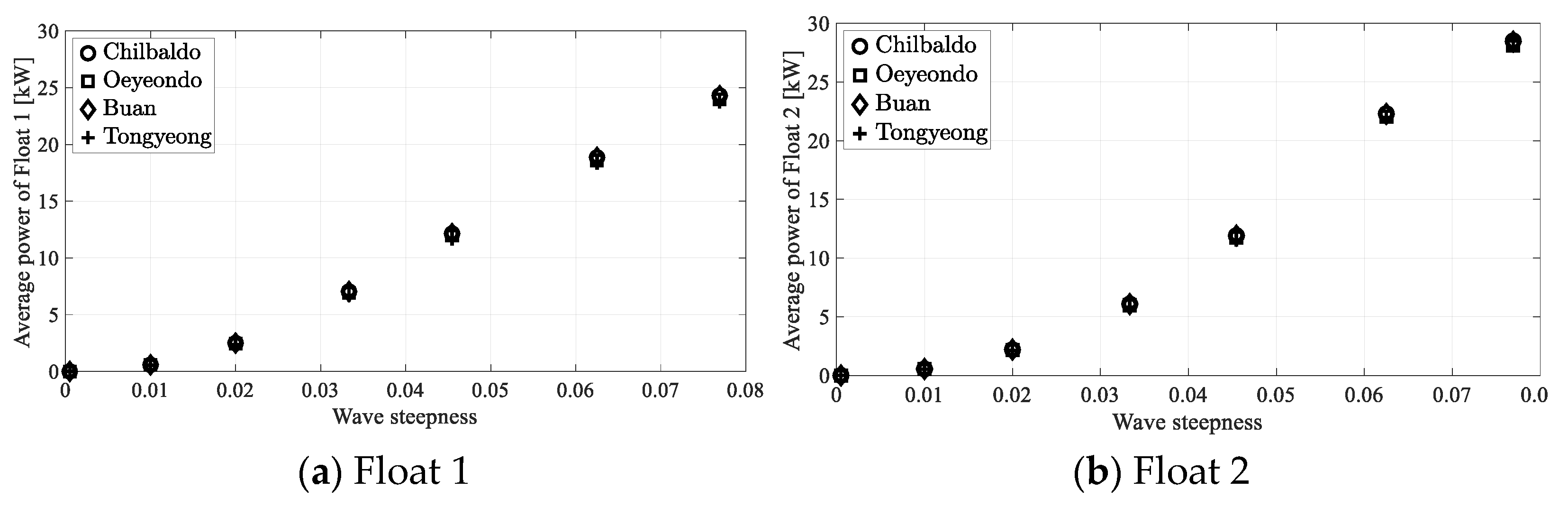
Figure 16 compares the average power production in each location according to the wave steepness with the environmental conditions given in Table 2. The magnitude and trends of average power production were similar in all locations. When the wave steepness is greater than 0.0455, the average power production of Float 2 is greater than that of Float 1. This is because the pitch RAO of Float 2 increases in this range.

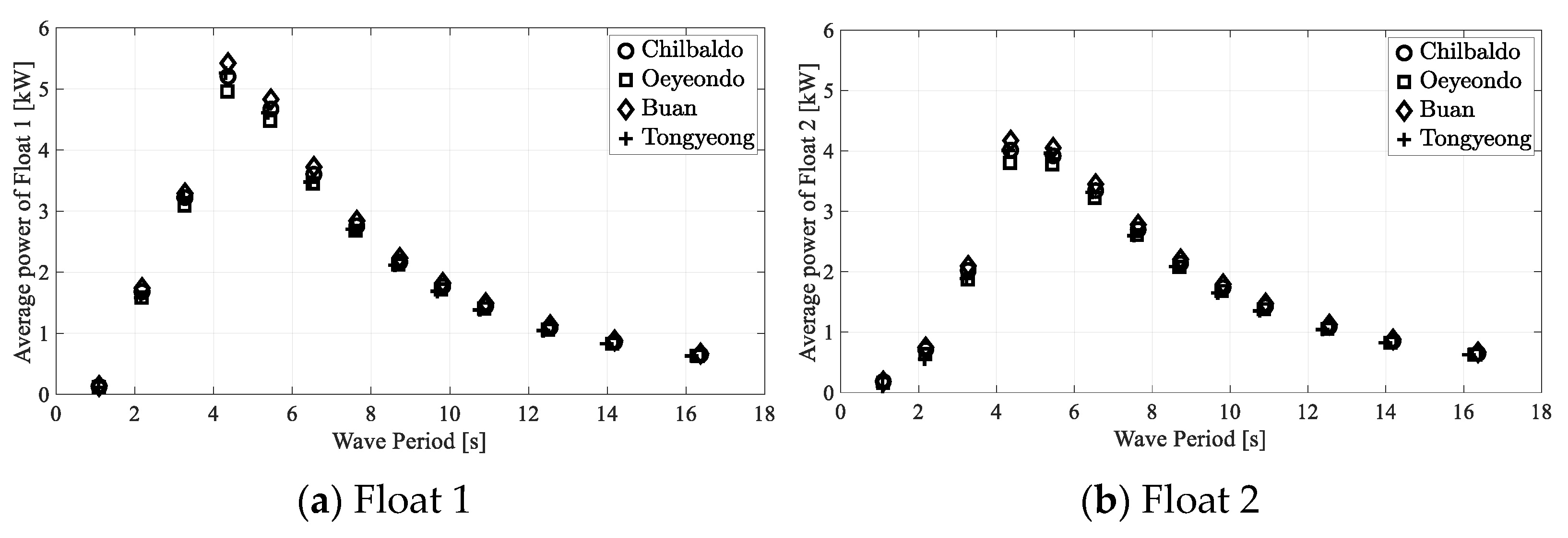
Figure 17 compares the average power production according to the wave period, with the wave height given for each location. The average power production tends to converge to zero in the low wave period (high frequency), has a maximum value at the wave period of four seconds, and then converges to zero in the high wave period (low frequency).

This trend is closer to the heave RAO of a general floating body. The highest and lowest average power production were found in Buan and Oeyeondo, respectively. This is because the wave height at Buan is approximately 4% greater than that at Oeyeondo. On the other hand, the average power production of Float 1 (rear body) was greater than that of Float 2 in most wave periods.

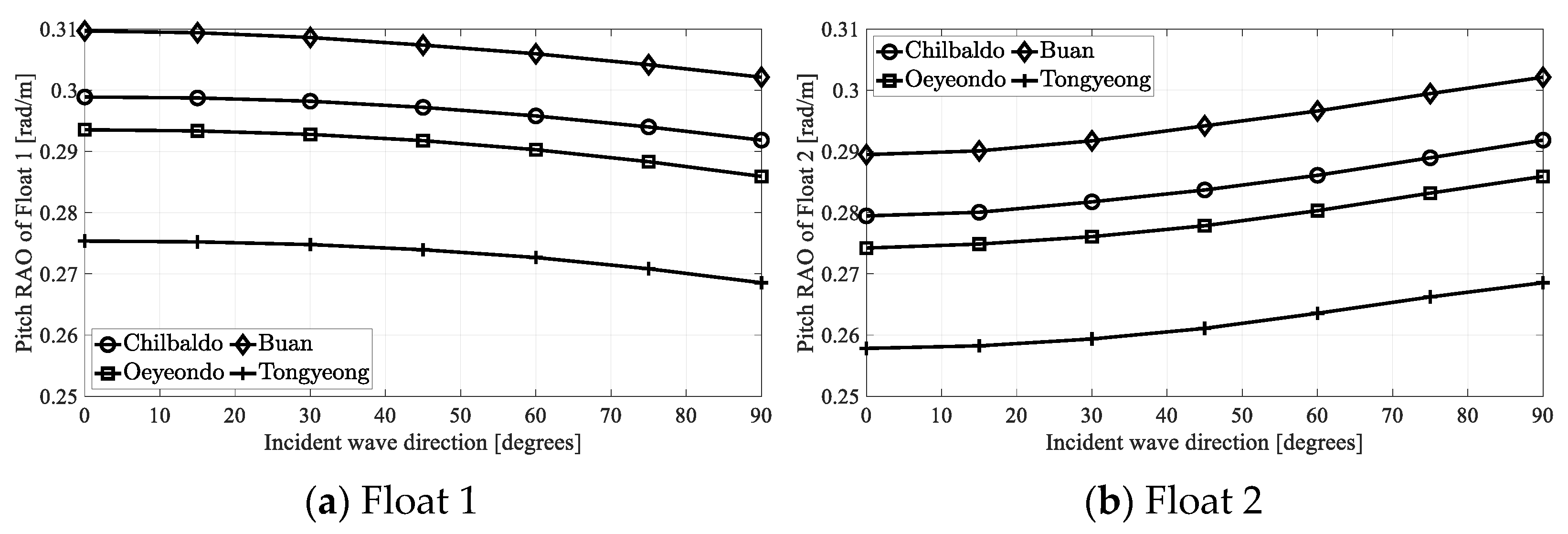
The results under actual sea conditions were analyzed by applying the wave height and wave period presented in Table 2. The motion and power production of the float were affected significantly by the propagation direction of the incident wave. Figure 18 compares the pitch RAO according to the direction of the incident wave. As the direction of the incident wave changed from 0° to 90°, the pitch RAO decreased gradually in Float 1 (rear body) and increased gradually in Float 2 (front body). Furthermore, the magnitude of the pitch RAO was the largest in Buan. This is because the incident wave power is the largest in Buan among the four selected locations in real sea situations.

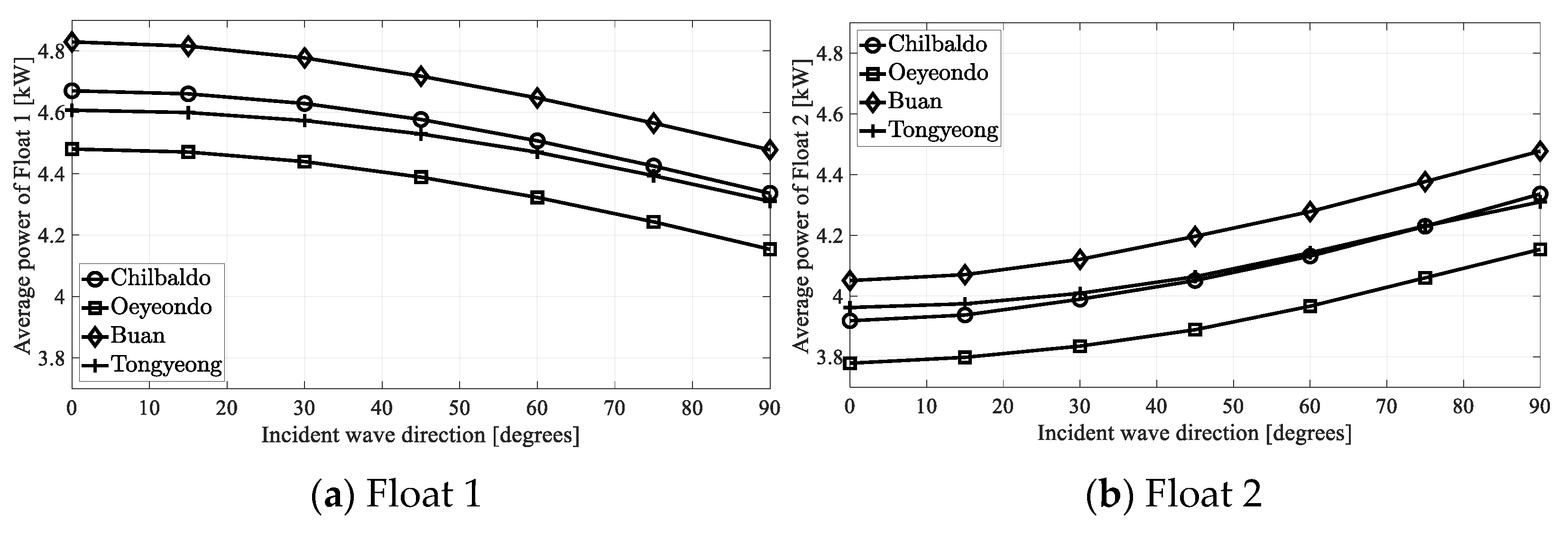
Figure 19 compares the average power production of the four locations for various incident wave directions. As in the comparison of pitch RAO (Figure 18), Buan had the largest average power production, whereas Oeyeondo had the smallest, which is a different trend from the pitch RAO comparison. This shows that large rotational displacement of the float does not necessarily mean large power production.

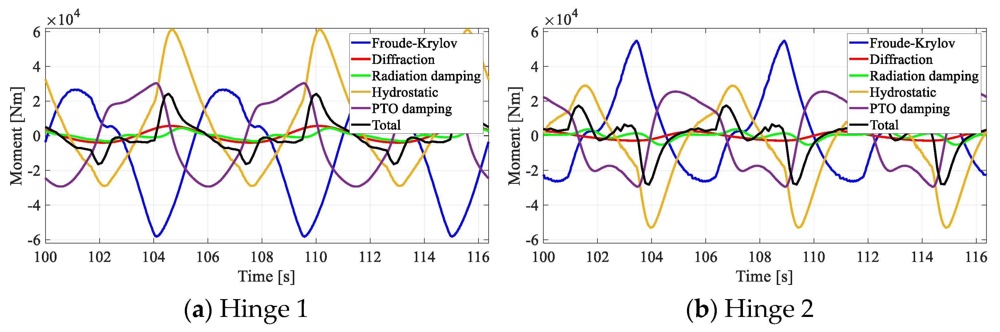
The magnitude of the pitch RAO between the two floats may vary depending on the environmental conditions (Figure 15). To analyze why the result of Float 1 (rear buoy) is greater than that of Float 2 (front buoy) under given environmental conditions, each component of moment acting on the hinge point was compared. In Figure 20, the mean absolute values of the total moments for each hinge point of the buoy were compared. The mean absolute value of Float 1 (calculated result:$1.0835\times {10}^5$ Nms) was greater than that of Float 2 (calculated result: $1.0128\times {10}^5$ Nms). This means that the change in angular velocity of Float 1 is larger than that of Float 2, and the angular velocity and rotational displacement are also larger.

In both floats, the moment caused by Froude–Krylov force and hydrostatic force had a large influence. On the other hand, the moment caused by diffraction and radiation damping forces had little effect on the magnitude of the total moments. The moment components canceled each other out, so that the mean absolute value of the total moment had a relatively small value.

Table 5. Average power, CWR, and peak power at each location with a 0° wave direction.

Location	Average Power (kW)		CWR		Peak Power (kW)
	Float 1	Float 2	Float 1	Float 2	Float 1	Float 2
Chilbaldo	4.61	3.92	0.271	0.230	9.29	8.75
Oeyeondo	4.48	3.78	0.278	0.235	8.81	8.35
Buan	4.83	4.05	0.276	0.231	9.67	9.14
Tongyeong	4.61	3.96	0.284	0.244	9.10	8.69

summarizes the average power, CWR, and peak power at each location when the incident wave direction angle is 0°. The power production varied by up to 20% between the front and rear float, depending on the incident wave direction. Overall, it showed a larger value in Float 1 (rear body) than in Float 2 (front body). This means that the power production efficiency is higher with Float 1 than Float 2 under the given environmental conditions.

As mentioned earlier, Buan had the largest power production among the four sites, followed by Chilbaldo. If installation and maintenance are not considered, Buan is the most suitable place to operate a Wavestar-type WEC. On the other hand, the water depth of Buan is approximately 51% deeper than that of Chilbaldo, and the difference in power generation between the two locations is less than 5%. Therefore, it is necessary to select a suitable site considering all installation and maintenance costs and power production.

4. Conclusions

In this study, a numerical procedure for the three-dimensional time-domain motion analysis of floating bodies for Korean nearshore areas was developed using an augmented formulation, an example of a multibody dynamics formulation. Time-domain analysis was carried out, applying the linear and weakly nonlinear hydrodynamic analysis methods.

The six-year wave data for Korean nearshore areas were obtained from the Korea Meteorological Administration. Based on them, four locations with environmental conditions suitable for Wavestar-type WECs were selected: Chilbaldo, Oeyeondo, Buan, and Tongyeong. The rotational motions and wave power production of the WECs were analyzed. The important results of the analysis are as follows:

1. Linear time-domain analysis for hydrodynamic assessments is unsuitable for an the analysis of HPA-type WECs. This is because the nonlinear Froude–Krylov and hydrostatic forces according to the relative position between the floating body and the water surface significantly affect the body motion.

2. When two floats are installed parallel to each other in opposite directions, the wave power production for various wave periods showed a similar tendency to the heave RAO of a general floating body. The average power production of Float 1 (rear body) was greater than that of Float 2 (front body) in most wave periods.

3. When the real sea conditions were applied, the power production differed by up to 20% depending on the incident wave direction.

4. Among the four locations selected, Buan showed the largest power production, followed by Chilbaldo. If installation and maintenance are not considered, Buan is the most suitable place to operate a Wavestar-type WEC. On the other hand, it is necessary to select a suitable site considering all installation and maintenance costs in addition to power production.

A more detailed study, including directional irregular waves, will be carried out in the future.

References

- Clément, A.; McCullen, P.; Falcão, A.; Fiorentino, A.; Gardner, F.; Hammarlund, K.; Lemonis, G.; Lew-is, T.; Nielsen, K.; Petroncini, S.; et al. Wave energy in europe: Current status and perspectives. Renew. Sustain. Energy Rev. 2002, 6, 405–431. [Google Scholar] [CrossRef]
- Drew, B.; Plummer, A.R.; Sahinkaya, M.N. A review of wave energy converter technology. Proc. Inst. Mech. Eng. Part A J. Power Energy 2009, 223, 887–902. [Google Scholar] [CrossRef] [Green Version]
- Falcão, A. Wave energy utilization: A review of the technologies. Renew. Sustain. Energy Rev. 2010, 14, 899–918. [Google Scholar] [CrossRef]
- Babarit, A.; Hals, J.; Muliawan, M.; Kurniawan, A.; Moan, T.; Krokstad, J. Numerical bench-marking study of a selection of wave energy converters. Renew. Energy 2012, 41, 44–63. [Google Scholar] [CrossRef]
- Aderinto, T.; Hua, L. Ocean wave energy converters: Status and challenges. Energies 2018, 11, 1250. [Google Scholar] [CrossRef] [Green Version]
- Sugiura, K.; Sawada, R.; Nemoto, Y.; Haraguchi, R.; Asai, T. Wave flume testing of an oscillating-body wave energy converter with a tuned inerter. Appl. Ocean Res. 2020, 98, 102127. [Google Scholar] [CrossRef] [Green Version]
- Liu, C.; Chen, R.; Zhang, Y.; Wang, L.; Qin, J. A novel single-body system for direct-drive wave energy converter. Int. J. Energy Res. 2021, 45, 7057–7069. [Google Scholar] [CrossRef]
- Kramer, M.; Marquis, L.; Frigaard, P. Performance evaluation of the wavestar prototype. In Proceedings of the 9th European Wave and Tidal Energy Conference, Southampton, UK, 5–9 September 2011. [Google Scholar]
- Karimirad, M. Offshore Energy Structures: For Wind Power, Wave Energy and Hybrid Marine Platforms; Springer: Cham, Switzerland, 2014; pp. 223–249. [Google Scholar]
- Zurkinden, A.S.; Ferri, F.; Beatty, S.; Kofoed, J.P.; Kramer, M. Nonlinear numerical modeling and experimental testing of a point absorber wave energy converter. Ocean Eng. 2014, 78, 11–21. [Google Scholar] [CrossRef]
- Kim, S.J.; Koo, W.; Min, E.H.; Jang, H.; Youn, D.; Lee, B. Experimental Study on Hydrodynamic Performance and Wave Power Takeoff for Heaving Wave Energy Converter. J. Ocean Eng. Technol. 2016, 30, 361–366. [Google Scholar] [CrossRef] [Green Version]
- Wang, L.; Kolios, A.; Cui, L.; Sheng, Q. Flexible multibody dynamics modelling of point-absorber wave energy converters. Renew. Energy 2018, 127, 790–801. [Google Scholar] [CrossRef]
- Heo, S.; Koo, W. Numerical procedures for dynamic response and reaction force analysis of a heaving-point absorber wave energy converter. Ocean Eng. 2020, 107070. [Google Scholar] [CrossRef]
- Ghafari, H.R.; Neisi, A.; Ghassemi, H.; Iranmanesh, M. Power production of the hybrid Wavestar point absorber mounted around the Hywind spar platform and its dynamic response. J. Renew. Sustain. Energy 2021, 13, 033308. [Google Scholar] [CrossRef]
- Korean Ministry of Trade, Industry and Energy. New and Renewable Energy 3020 Implementation Plan; Korean Ministry of Trade, Industry and Energy: Sejong-si, Korea, 2017. (In Korean)
- Korean Ministry of Trade, Industry and Energy. The 8th Basic Plan for Long-Term Electricity Supply and Demand (2017–2031); Korean Ministry of Trade, Industry and Energy: Sejong-si, Korea, 2017.
- Singh, P.M.; Chen, Z.; Choi, Y.D. 15kW-class wave energy converter floater design and structural analysis. J. Korean Soc. Mar. Eng. 2016, 40, 146–151. [Google Scholar] [CrossRef]
- Kim, G.; Jeong, W.M.; Lee, K.S.; Jun, K.; Lee, M.E. Offshore and nearshore wave energy assessment around the Korean Peninsula. Energy 2011, 36, 1460–1469. [Google Scholar] [CrossRef]
- Kim, G.; Lee, M.E.; Lee, K.S.; Park, J.S.; Jeong, W.M.; Kang, S.K.; Soh, J.G.; Kim, H. An overview of ocean renewable energy resources in Korea. Renew. Sustain. Energy Rev. 2012, 16, 2278–2288. [Google Scholar] [CrossRef]
- Eum, H.S.; Jeong, W.M.; Chang, Y.S.; Oh, S.H.; Park, J.J. Wave Energy in Korean Seas from 12-Year Wave Hindcasting. J. Mar. Sci. Eng. 2020, 8, 161. [Google Scholar] [CrossRef] [Green Version]
- Ahn, S.; Ha, T. Characterization of wave energy resource hotspots and dominant wave energy systems in South Korean coastal waters. J. Clean. Prod. 2021, 309, 127202. [Google Scholar] [CrossRef]
- Kim, J.; Kweon, H.M.; Jeong, W.M.; Cho, I.H.; Cho, H.Y. Design of the dual-buoy wave energy converter based on actual wave data of East Sea. Int. J. Naval Arch. Ocean Eng. 2015, 7, 739–749. [Google Scholar] [CrossRef] [Green Version]
- Ko, H.S.; Kim, S.; Bae, Y.H. Study on Optimum Power Take-Off Torque of an Asymmetric Wave Energy Converter in Western Sea of Jeju Island. Energies 2021, 14, 1449. [Google Scholar] [CrossRef]
- Kim, S.J.; Koo, W. Numerical Study on a Multibuoy-Type Wave Energy Converter with Hydraulic PTO System Under Real Sea Conditions. IEEE J. Ocean. Eng. 2021, 46, 573–582. [Google Scholar] [CrossRef]
- Lee, C.H. WAMIT Theory Manual. Report No. 95-2; Department of Ocean Engineering, Massachusetts Institute of Technology: Cambridge, MA, USA, 1995. [Google Scholar]
- Shabana, A.A.; Hussein, B.A. A two-loop sparse matrix numerical integration procedure for the solution of differential/algebraic equations: Application to multibody systems. J. Sound Vib. 2009, 327, 557–563. [Google Scholar] [CrossRef]
- Park, J.H.; Shin, M.S.; Jeon, Y.H.; Kim, Y.G. Simulation-Based Prediction of Steady Turning Ability of a Symmetrical Underwater Vehicle Considering Interactions Between Yaw Rate and Drift/Rudder Angle. J. Ocean Eng. Technol. 2021, 35, 99–112. [Google Scholar] [CrossRef]
- Shabana, A.A. Dynamics of Multibody Systems, 4th ed.; Cambridge University Press: Cambridge, UK, 2013. [Google Scholar]
- Zhang, L.; Zhang, D. A two-loop procedure based on implicit Runge–Kutta method for index-3 DAE of constrained dynamic problems. Nonlinear Dyn. 2016, 85, 263–280. [Google Scholar] [CrossRef]
- Guo, X.; Zhang, D.G.; Li, L.; Zhang, L. Application of the two-loop procedure in multibody dynamics with contact and constraint. J. Sound Vib. 2018, 427, 15–27. [Google Scholar] [CrossRef]
- Penalba, M.; Giorgi, G.; Ringwood, J.V. Mathematical modelling of wave energy converters: A review of nonlinear approaches. Renew. Sustain. Energy Rev. 2017, 78, 1188–1207. [Google Scholar] [CrossRef] [Green Version]
- Giorgi, G.; Penalba, M.; Ringwood, J. Nonlinear hydrodynamic models for heaving buoy wave energy converters. In Proceedings of the 3rd Asian Wave and Tidal Energy Conference, Singapore, 25–27 October 2016; pp. 144–153. [Google Scholar]
- Cummins, W.E. The impulse response function and ship motions. In Proceedings of the Symposium on Ship Theory, Hamburg, Germany, 25–27 January 1962. [Google Scholar]
- Ogilvie, T. Recent progress towards the understanding and prediction of ship motions. In Fifth Symposium on Naval Hydrodynamics; 1964; Volume 1, pp. 2–5. Available online: https://repository.tudelft.nl/islandora/object/uuid:5accdabd-b484-4450-9613-e1d2c5ee211e?collection=research (accessed on 22 June 2021).
- Kim, D.; Poguluri, S.K.; Ko, H.S.; Lee, H.; Bae, Y.H. Numerical and experimental study on linear behavior of salter’s duck wave energy converter. J. Ocean Eng. Technol. 2019, 33, 116–122. [Google Scholar] [CrossRef] [Green Version]
- Wei, Y.; Barradas-Berglind, J.J.; Yu, M.; van Rooij, M.; Prins, W.A.; Jayawardhana, B.; Vakis, A.I. Frequency-domain hydrodynamic modelling of dense and sparse arrays of wave energy converters. Renew. Energy 2019, 135, 775–788. [Google Scholar] [CrossRef]
- Wendt, F.F.; Yu, Y.-H.; Nielsen, K.; Ruehl, K.; Bunnik, T.; Touzon, I.; Nam, B.W.; Kim, J.S.; Kim, K.-H.; Janson, C.E.; et al. International Energy Agency Ocean Energy Systems Task 10 Wave Energy Converter Modelling Verification and Validation. In Proceedings of the 12th European Wave and Tidal Energy Conference, Technical Committee of the European Wave and Tidal Energy conference, Cork, Ireland, 27 August–1 September 2017. [Google Scholar]
- Flavià, F.F.; Babarit, A.; Clément, A.H. On the numerical modeling and optimization of a bottom-referenced heave-buoy array of wave energy converters. Int. J. Mar. Energy 2017, 19, 1–15. [Google Scholar] [CrossRef] [Green Version]
- Korea Meteorological Administration, Portal for Korea Meteorological Open Data. Available online: https://data.kma.go.kr/data/sea/selectBuoyRltmList.do?pgmNo=52 (accessed on 22 June 2021). (In Korean).
- Cho, I.H. Effect of Internal Fluid Resonance on the Performance of a Floating OWC Device. J. Ocean Eng. Technol. 2021, 35, 216–228. [Google Scholar] [CrossRef]
- ANSYS. Aqwa Theory Manual; ANSYS, Inc.: Canonsburg, PA, USA, 2021. [Google Scholar]
Figure 1.
Description of a Wavestar-type WEC platform applied in this study.
Figure 2.
Two-loop procedure for the implicit time-integration method.
Figure 3.
Model of a spherical float.
Figure 4.
Comparison of the heave free-decay test (5.0 m initial displacement).
Figure 5.
Comparison of heave RAO of the sphere with PTO damping (wave steepness = 0.0628).
Figure 6.
Model description of a spherical float.
Figure 7.
Comparison of pitch RAO of the float according to the incident wave direction ( = 1.4 rad/s).
Figure 8.
Selected wave buoy locations in the Korean nearshore areas: Chilbaldo, Oeyeondo, Buan, and Tongyeong.
Figure 9.
Model description of an HPA-type WEC model with a single hemispherical float constrained to a hinge point.
Figure 10.
Average power production of the float according to the PTO extraction coefficient.
Figure 11.
Time history results of the single float at Chilbaldo.
Figure 12.
Model description of a two-buoy HPA-type WEC with constrained hinge points.
Figure 13.
Comparison of the added mass and radiation damping coefficients of the float at Chilbaldo.
Figure 14.
Comparison of the pitch RAO according to the distance between hinge points at Chilbaldo (H = 1.26 m, T = 5.46 s).
Figure 15.
Comparison of the Pitch RAO assessed using linear and weakly-nonlinear analysis according to the wave steepness.
Figure 16.
Comparison of the average power production of each location according to the wave steepness.
Figure 17.
Comparison of the average power production of each location according to the wave periods.
Figure 18.
Comparison of the pitch RAO according to the incident wave directions at each location.
Figure 19.
Comparison of average power production according to the incident wave directions at each location.
Figure 20.
Time history of moment components acting on the hinge points in the Buan area.