
MRlogP: Transfer Learning Enables Accurate logP Prediction Using Small Experimental Training Datasets


School of Biological Sciences, University of Edinburgh, The King’s Buildings, Edinburgh EH9 3BF, Scotland, UK
*
Authors to whom correspondence should be addressed.
Processes 2021, 9(11), 2029; https://0-doi-org.brum.beds.ac.uk/10.3390/pr9112029
Submission received: 27 July 2021
/
Revised: 20 October 2021
/
Accepted: 10 November 2021
/
Published: 13 November 2021
(This article belongs to the Special Issue Molecular Modeling: Computer-Aided Drug Design)
Abstract
:Small molecule lipophilicity is often included in generalized rules for medicinal chemistry. These rules aim to reduce time, effort, costs, and attrition rates in drug discovery, allowing the rejection or prioritization of compounds without the need for synthesis and testing. The availability of high quality, abundant training data for machine learning methods can be a major limiting factor in building effective property predictors. We utilize transfer learning techniques to get around this problem, first learning on a large amount of low accuracy predicted logP values before finally tuning our model using a small, accurate dataset of 244 druglike compounds to create MRlogP, a neural network-based predictor of logP capable of outperforming state of the art freely available logP prediction methods for druglike small molecules. MRlogP achieves an average root mean squared error of 0.988 and 0.715 against druglike molecules from Reaxys and PHYSPROP. We have made the trained neural network predictor and all associated code for descriptor generation freely available. In addition, MRlogP may be used online via a web interface.
1. Introduction
Common rulesets used in drug discovery and medicinal chemistry, such as Lipinski’s “rule of five” [1,2] and Oprea’s “rule of three” [3,4], aggregate properties of a molecule to predict a further property such as in-vivo absorption or how ‘lead like’ and suitable for medicinal chemistry efforts a molecule is. Central to many rulesets and compound filtering criteria is lipophilicity, a measure of a unionized compound’s ability to dissolve or be held in hydrophobic versus a polar solvent [5]. Compound lipophilicity is commonly expressed as the log of the partition coefficient of compound distribution in an octanol/water system and commonly referred to as logP. Assessing the partition coefficient on a log scale gives rise to hydrophobic compounds having a positive logP and hydrophilic compounds having a negative logP. Along with aggregation of this value with other properties as input to predictors, it is also used on its own to perform in-vivo localization [6] and barrier permeability predictions [7]. Hann and Keserü assessed approved drugs and identified logP along with molecular weight as strong predictors of a compound achieving approved drug status [8]. Experimental determination of logP can be performed using a range of methods. However, certain cases exist where experimental determination is difficult. In addition, the case for logP prediction on virtual compounds is compelling. Often, medicinal chemistry efforts use calculated logP values to guide derivatization within structural activity relationship exploration, each derivative having its logP predicted before moving to costly synthesis and allowing efforts to be focused on only the most promising compounds.
1.1. Prediction of logP
Methods of logP prediction can be broadly placed into two classes, substructure and whole molecule approaches [9], each class separated by one fundamental assumption, that a molecule’s lipophilicity is additive, or that it is not, and it is more complex than simply a sum of discrete substructure contributions. These substructures may be large moieties such as ring systems, or smaller features such as atoms. Many freely-available logP predictors are available, including substructure-based methods, such as ALOGP [10], XLOGP3 [11], and JPlogP [12], along with programs using whole molecule methods such as ALOGPS [13], MLOGP [14], VEGA [15], and UFZ-LSER [16]. Both ALOGP [10] and XLOGP3 [13] adopted an atom-additive method for logP prediction, whereas XLOGP3 [13] utilizes larger molecular fragments, applying further correction factors to deal with intramolecular interactions. Unlike substructure-based methods, MLOGP [14] uses 13 1D-topological parameters to represent whole molecules via a multiple regression model. VEGA [15] predicts logP values by considering the entire molecular graph and approximating intermolecular interactive forces and their correlation to lipophilicity. UFZ-LSER [16] uses an empirical treatment of molecular descriptors representing the entire molecule. Mannhold et al. [17] evaluated and compared the performance of 30 logP predictors against one public and two in-house datasets, discovering that a consensus model using the average of predictions from top-ranked models outperformed the majority of predictors evaluated. Observing the predictive power of consensus logP predictions, Plante et al. used consensus logP values in the creation of the substructure-based method JPlogPcoeff [12]. JPlogPcoeff is trained on the mean of predicted logPs for 89,517 diverse molecules from four freely available approaches (ALOGP [10], XLOGP2 [18], XLOGP3 [11], and SlogP [19]). Linear regression was used to fit coefficients for pre-defined atom-types relevant to logP prediction. Beyond this parameterised model, a further predictor JPlogPlibrary [12] was developed which includes a correction step, adding contributions from molecules similar to the prediction target from experimental data in the PHYSPROP dataset [20].
Both JPlogPcoeff and JPlogPlibrary are shown to outperform the majority of logP predictors when evaluated using their chosen high quality external test set containing experimentally measured logPs for 707 molecules as created and published by Martel et al. [21].
1.2. Motivation for This Study
Building upon the value of consensus predictions identified by Mannhold et al. and the demonstration by Plante that real world data can be used to further improve predictors trained on non-experimental data, we set out to determine if modern machine learning techniques could outcompete expertly crafted systems exploiting specialist chemical knowledge as well as improving upon machine learning derived systems created at the beginning of the current machine learning/AI revolution. In this work, we chose to add emphasis on usability for drug discovery and medicinal chemistry where accurate logP predictions will have the most impact, focusing prediction optimization efforts within druglike chemical space. Whilst subjective, a convenient and widely used cheminformatics-based measure of druglikeness exists in the quantitative estimate of drug-likeness (QED) score [22] as developed by Bickerton et al., ranging between 0 and 1 with a score above 0.67 indicative of a druglike molecule. This quantification of druglikeness greatly improves on previous ‘rule of thumb metrics’ such molecular weights between 150 and 500 Da, and a specified number of hydrogen bond donors and acceptors. Examples of predictors tailored to areas of chemical space can be found in literature with foci on peptides and certain compound substructure classes [23]. The ultimate goal of our work was the creation of an open, freely available, performant druglike small molecule logP predictor allowing easy integration into existing drug discovery pipelines and also deployed on the web for rapid, iterative, and design-led use.
2. Materials and Methods
All code and derived datasets are available within the MRlogP source repository under an open-source license, available at https://github.com/JustinYKC/MRlogP (accessed on 23 July 2021). Dataset preparation, model training, and predictions were carried out on a server with an Intel i7 8700 CPU, 32 GB RAM, and an NVIDIA GeForce RTX 2080 to accelerate training, running Ubuntu 18.04.
2.1. Dataset Preparation
Our training, validation, and test sets described below all underwent the following filters and transformations through custom Python (version 3.7.9) code calling RDKit [24] (Version 2020.09.1.0): salt removal, standardization, uniquification, removal of molecules containing disallowed atoms, retaining only C, N, O, S, F, Cl, Br, I, B, Si, and P atom containing molecules, MW ≤ 800, removal of pan assay interference compounds (PAINS) [25,26], and finally the removal of molecules with QED [22] scores less than 0.67. Molecules were represented as sets of molecular descriptors, capturing (i) atom connectivity with the circular Morgan fingerprint [27] as implemented in RDKit (version 2017.03.3), (ii) larger moieties using the FP4 fingerprint as implemented in OpenBabel (version 2.4.1) [28] and Pybel [29] (version 0.15.3), and finally (iii) 3D shape and electrostatics using the USRCAT [30] molecular descriptor sets, as implemented in RDKit (version 2017.03.3). USRCAT descriptors require generation of a single low energy conformer which was achieved using RDKit and the techniques described by Ebejer et al. [31]. See source repository for all code and resultant datasets for training, validation, and prediction.
Our training set, which we refer to as the 500k set, is derived from the 2019-05 release of the eMolecules database, obtained from www.eMolecules.com (accessed on 22 May 2019) and processed using the filtering and transformation steps defined above. ALOGP [10], XLOGP2 [18], XLOGP3 [11], and SlogP [19] were used to predict logPs for each molecule within the training set, which were then recorded and used to produce a Pandas (Version 1.2.1) dataframe. The analysis revealed an average standard deviation across the four logP predictors to be 0.415. To keep only molecules where a good consensus for the predicted logP was achieved, molecules with consensus prediction standard deviations greater than 2 times the average standard deviation were removed. This reduced the dataset size to 20,545,077 molecules, a surprisingly small reduction, indicating good agreement between the chosen logP predictors. Molecules were then placed in bins according to their average predicted logP, each bin spanning one log unit from −5 to 10 (the chosen prediction range of our logP predictor). In preparation for the application of diversity picking a set number of molecules from each bin to create as flat as possible a distribution of molecules across all bins, a simple algorithm was applied. Requesting 500,000 molecules across the logP range spanned by 15 single log unit bins would ideally produce bins contain 33,333 molecules each. However, extreme bins, such as those containing logPs of -5 to -4, and 9 to 10 contained only 4 and 7 molecules, respectively. To reach the target 500,000 molecules, more are therefore evenly taken from every other bin. Our target pick size from the bins spanning logPs from −5 to 10 contained 4, 9, 36, 18,290, 361,002, 1,767,551, 3,742,630, 4,446,441, 2,851,614, 848,808, 83,180, 1678, 62, 17, and 7 molecules, respectively (see Supplementary Figure S1). Morgan fingerprints for all molecules were used as input to the RDKit MaxMinPicker, allowing diverse picking of molecules from within bins. Conformer generation failed on a small number of molecules with problems such as incorrect bond orders, leaving our training dataset containing 498,426 molecules. For the sake of brevity, we will refer to this as the 500k training dataset.
The Martel_DL dataset comprises 244 druglike filtered molecules from the high quality experimentally determined logP dataset as published by Martel et al. [21]. All logP data in this dataset were obtained using ultra-high-performance liquid chromatography. Standard filters, transformations, and descriptor generation steps defined above were applied to generate this Martel_DL (DrugLike) dataset (see Supplementary Table S5).
The Physprop_DL dataset contains 5638 molecules captured, filtered and transformed using the dataset and descriptor generation steps above from the EPA’s (United State Environmental Protection Agency, Washington, WA, USA) EPI software (http://esc.syrres.com/interkow/EpiSuiteData_ISIS_SDF.htm), known as PHYSPROP and used extensively in the creation of historically widely used logP predictors.
The Reaxys_DL test set comprises 20,067 molecules from Reaxys [32], an online web-based chemistry database containing more than 500 million published experimental values derived predominantly from medicinal chemistry and drug discovery programs.
2.2. Neural Network Architecture and Hyperparameters
We utilized a fully connected artificial neural network (ANN) in this study with the goal of developing a predictor of logP tuned and highly accurate in predictions for druglike small molecules. Defined in Python (version 3.7.9) using Keras (version 2.2.4), TensorFlow (version 2.2.0), and cuDNN (version 7.6.5), a 5-layer sequential model was constructed, comprising 1 input layer of 316 nodes to represent a molecule (128 values from FP4, 128 from ECFP4 and 60 from USRCAT), 3 hidden layers with variable numbers of nodes within each to be optimized in hyperparameter scanning, and a single node output layer. A parametric rectified linear unit (PReLU) and leaky rectified linear unit (LeakyReLU) were employed over the commonly used ReLU activation functions to avoid non-zero gradients and poor training performance [33]. Furthermore, a simple linear activation function was used on the output layer to scale network outputs. Mean squared error (MSE) was used as a loss function for the Adam optimizer with dropout rate applied during network training. A simple grid search approach was taken to hyperparameter scanning for optimization of the number of hidden layers, nodes per hidden layer, batch size, number of training epochs, dropout rate, and learning rates. Model performance in the hyperparameter scan was evaluated using root mean square error (RMSE), as shown in Equation (1).
where n is the number of molecules in the dataset, h is our prediction function which outputs a logP value for the i-th molecule in a dataset based on its features x, and y is the measured logP value for the i-th molecule.
The final representative RMSE was then calculated as the average of three repeats. Each repeat used a randomized 90–10 train-test split holdout validation of the 500k dataset ensuring the number of validated molecules for each logP range remained proportional to the number of training molecules within the 1 log unit range (see Supplementary Figure S1). During hyperparameter optimization, a total of 1944 neural networks were constructed, trained, and evaluated three times each with a shuffled dataset supplying training and test data for RMSE calculation. See Supplementary Table S1 for hyperparameters explored. The best 20 models, achieving the lowest average RMSE, were further reevaluated using 10-fold cross validation. With the best network hyperparameters identified and evaluated in 10-fold cross validation. The final network model was retrained using the entire 500k dataset. We evaluated top performing hyperparameter scan models after retraining, calculating RMSE values for the Martel_DL, Physprop_DL, and Reaxys_DL datasets (see results and Table 1).
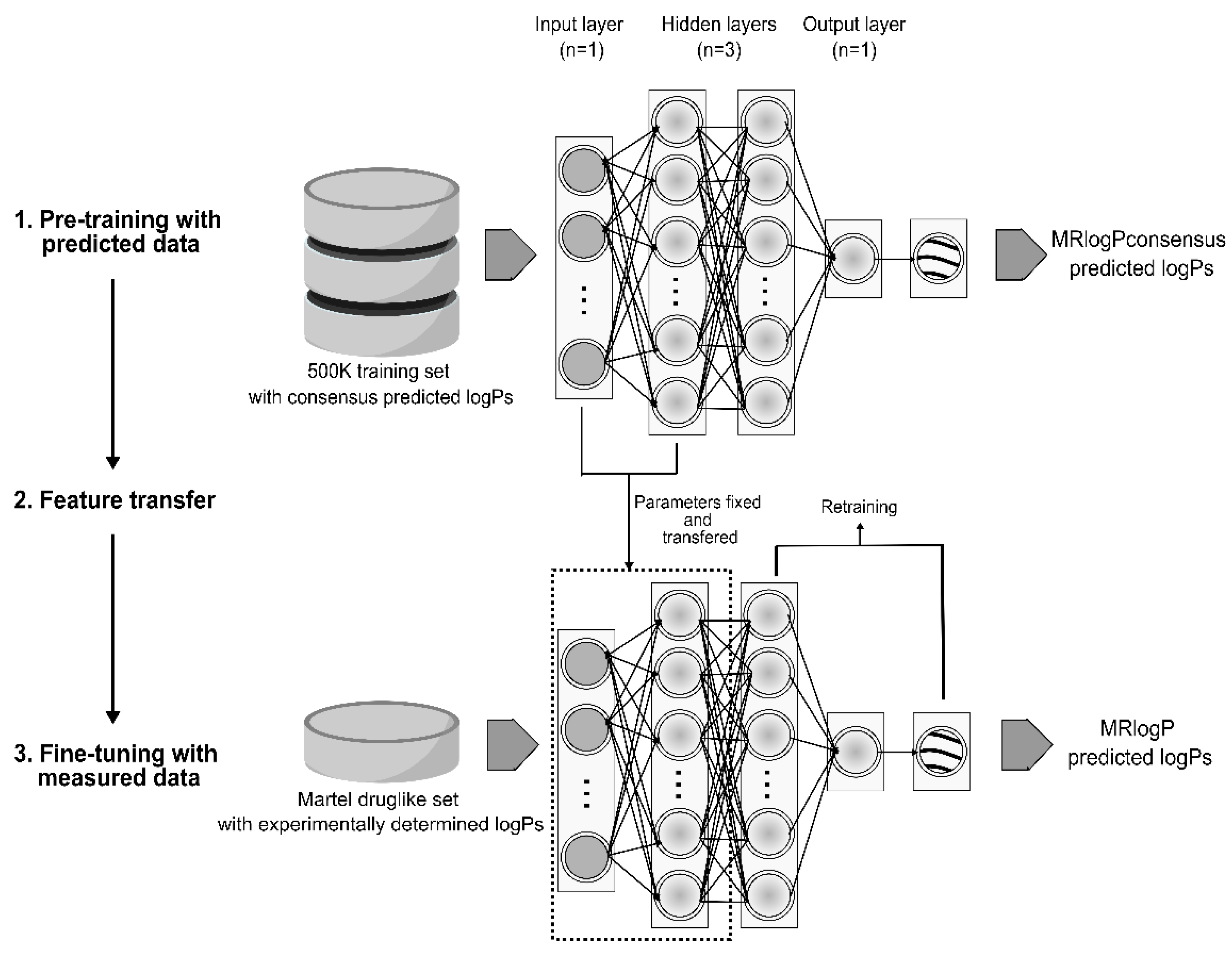
In order to further improve prediction performance and create the best predictor possible, techniques from transfer learning were applied using the highly accurate Martel_DL dataset (see Figure 1 for a schematic workflow representation). This essentially applied a small correction to our already well-performing model trained on consensus data, applying the small amount (244 molecules) of high-quality experimental data to converge on a better predictor. Before tweaking the weights in the hidden layers, the output layer of the pre-trained model was replaced with the new one, which was then trained to learn weights from the new data. In the course of transfer learning, each of the hidden layers in the pre-trained model were unfrozen and retrained on the new data set using a low learning rate (1.31 × 10⁻⁵) so as not to entirely overwrite weights set through training on the 500k dataset. Supplementary Table S4 shows the hyperparameters scanned for transfer learning in this study.
3. Results
3.1. Arteficial Neural Network Training and Validation on Consensus logPs
Performing three repeats of each set of hyperparameters (see methods) allowed averaging and prioritization of the top 20 parameter sets. These 20 models (see Supplementary Table S2) defined by their hyperparameters were then taken forward for 10-fold cross validation. All of these top 20 models had wide hidden layers, were trained with a high number of epochs (either 25 or 30) and a learning rate of 1 × 10⁻⁴, and had dropout rates of 0.1 or 0.2.
Cross validation showed the best performing model to have 5 layers (3 hidden layers along with input and output layers), 1264 nodes, a batch size of 32, trained for 30 epochs, a 0.2 dropout rate, and a 1 × 10⁻⁴ learning rate. Moreover, folds evaluated with this model were more homogeneously spread around the median without outliers and had smaller RMSEs within the interquartile range, indicating a robust and general model (see Supplementary Figure S2). The performance of this final model was evaluated against the three druglike test sets after retraining on the whole 500k dataset, achieving RMSEs of 0.972, 1.074, and 0.727 on Martel_DL, Reaxys_DL, and Physprop_DL, respectively (see Table 1). This final model was named MRlogPconsensus, indicating it was trained solely on consensus prediction data.
3.2. Transfer Learning
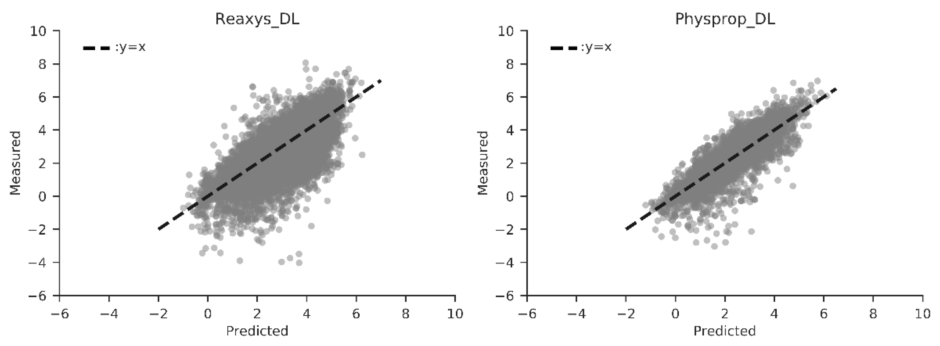
With MRlogPconsensus achieving an RMSE around 1 log unit, an improved model was achieved through application of transfer learning techniques (see Methods), correcting MRlogPconsensus using experimental data in the form of 244 molecules in the Martel_DL dataset. Transfer learning created an ANN predictor we term MRlogP, demonstrating an improvement on the remaining Reaxys_DL and Physprop_DL datasets, scoring 0.988, and 0.715, respectively (Table 1). Figure 2 shows MRlogP predicted logPs against measured logP values within the Reaxys_DL (left) and Physprop_DL (right) test sets. The high density of data points observed around the line for both Reaxys_DL and Physprop_DL measured logPs with negative values are, however, predicted with higher RMSE by MRlogP. This is most clearly shown for Reaxys, with a wide range of predicted logPs (0–4) for measured logP values between −2 and −5. This can be seen later in Figure 2 and Figure 3, with large RMSEs present in the most negative logP bins.
3.3. Performance Comparison
A performance comparison of MRlogP and MRlogPconsensus was carried out against, to our knowledge, and at the time, the best freely available logP predictor JPlogP as implemented in the Chemistry Development Kit (CDK) [34]. Table 1 shows performance of these three predictors against the three test sets. Martel_DL is left out of the MRlogP performance evaluation, as this predictor was cross trained on the dataset. MRlogPconsensus is able to outperform JPlogP on all of the three druglike test sets. Moreover, it outperforms JPlogP on the Reaxys_DL test set containing both negative and positive logPs more akin to the range encountered in medicinal chemistry and drug discovery programs. MRlogP improves the predictions further and demonstrates that small amounts of experimental data may be used to correct predictors built on low quality consensus predictions.
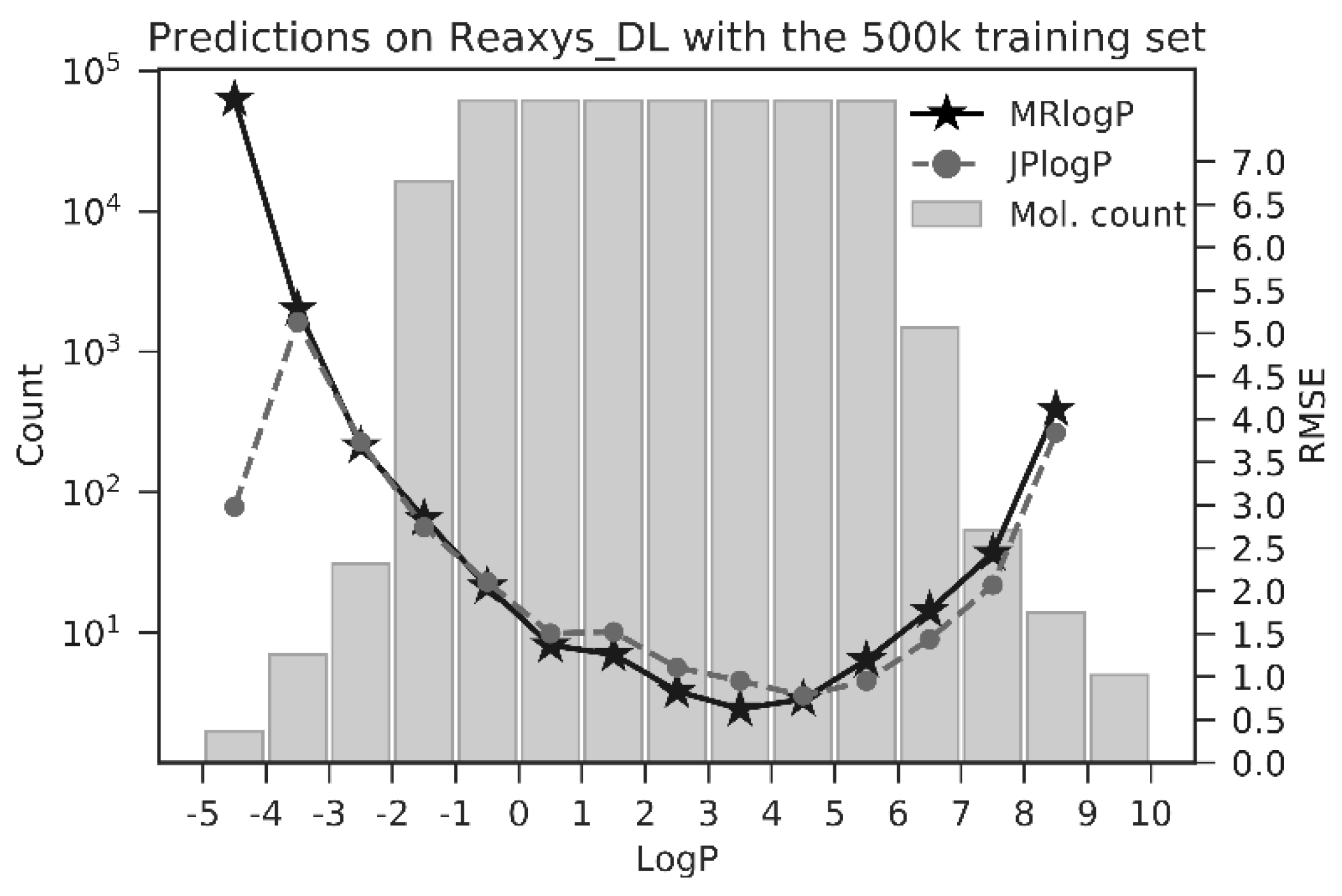
We may observe the impact that the abundance of training data has on predictor performance in Figure 3, showing the number of molecules within logP bins and predictor performance. This striking plot shows RMSE (as measured from the Reaxys_DL dataset) as expected to be inversely correlated with the number of molecules present within each logP bin. In short, ANNs are very good at making predictions concerning representations of molecules similar to those present in training sets. See Supplementary Figure S3 for similar training set bin occupancy along with predictor performance for the Physprop_DL dataset.
4. Discussion
We have created a logP predictor, optimized for molecules in druglike chemical space. We developed, to our knowledge, the best performing freely available druglike small molecule logP predictor. In addition, we demonstrated how relatively few experimental measurements may be used to perform a correction on models trained with consensus predicted data. This method essentially created a rough estimator of logP which is then refined using the highly accurate logP data present within the Martel et al. dataset. It is hoped that this work, whilst offering scientists the ability to perform more accurate predictions on their own molecules of interest, also opens further transfer learning possibilities for accurate physicochemical property prediction using limited high accuracy experimental measurement. MRlogP is available to run locally and for inclusion in existing drug discovery pipelines (all associated code freely available on GitHub at https://github.com/JustinYKC/MRlogP accessed on 23 July 2021), along with a simple and easy to use web-based version at https://similaritylab.bio.ed.ac.uk/mrlogp.
Supplementary Materials
The following are available online at https://www.mdpi.com/article/10.3390/pr9112029/s1, PDF document PDFS1: Supporting information.
Author Contributions
Conceptualization, S.S. and M.A.; methodology, S.S. and Y.-K.C.; programming: Y.-K.C. and S.S.; investigation, Y.-K.C.; resources, M.A.; data curation, Y.-K.C.; writing—original draft preparation, Y.-K.C. and S.S.; writing—review and editing, S.S., Y.-K.C. and M.A.; supervision, S.S. and M.A.; project administration, M.A.; funding acquisition, M.A. All authors have read and agreed to the published version of the manuscript.
Funding
The authors acknowledge financial support from the Scottish Universities Life Sciences Alliance (SULSA-http://www.sulsa.ac.uk), the Wellcome Trust (Grant 201531/Z/16/Z & ISSF3-SimilarityLab), and the Medical Research Council (MRC- www.mrc.ac.uk, J54359) Strategic Grant.
Institutional Review Board Statement
Not applicable.
Informed Consent Statement
Not applicable.
Data Availability Statement
All code, derived datasets, parameter sets and machine learning models are available within the MRlogP source repository under an open-source license, available at https://github.com/JustinYKC/MRlogP (accessed on 23 July 2021).
Conflicts of Interest
The authors declare no conflict of interest.
References
- Lipinski, C.A. Lead- and drug-like compounds: The rule-of-five revolution. Drug Discov. Today Technol. 2004, 1, 337–341. [Google Scholar] [CrossRef]
- Lipinski, C.A. Drug-like properties and the causes of poor solubility and poor permeability. J. Pharm. Toxicol. Methods 2000, 44, 235–249. [Google Scholar] [CrossRef]
- Oprea, T.I. Current trends in lead discovery: Are we looking for the appropriate properties? J. Comput. Aided. Mol. Des. 2002, 16, 325–334. [Google Scholar] [CrossRef] [PubMed]
- Oprea, T.I.; Allu, T.K.; Fara, D.C.; Rad, R.F.; Ostopovici, L.; Bologa, C.G. Lead-like, drug-like or “Pub-like”: How different are they? J. Comput. Aided. Mol. Des. 2007, 21, 113–119. [Google Scholar] [CrossRef] [Green Version]
- Sangster, J. Octanol-Water Partition-Coefficients of Simple Organic-Compounds. J. Phys. Chem. Ref. Data 1989, 18, 1111–1229. [Google Scholar] [CrossRef]
- Moerlein, S.M.; Laufer, P.; Stocklin, G. Effect of lipophilicity on the in vivo localization of radiolabelled spiperone analogues. Int. J. Nucl. Med. Biol. 1985, 12, 353–356. [Google Scholar] [CrossRef]
- Waring, M.J. Lipophilicity in drug discovery. Expert. Opin. Drug Discov. 2010, 5, 235–248. [Google Scholar] [CrossRef] [PubMed]
- Hann, M.M.; Keserü, G.M. Finding the sweet spot: The role of nature and nurture in medicinal chemistry. Nat. Rev. Drug Discov. 2012, 11, 355–365. [Google Scholar] [CrossRef]
- Mannhold, R.; van de Waterbeemd, H. Substructure and whole molecule approaches for calculating logP. J. Comput. Aided. Mol. Des. 2001, 15, 337–354. [Google Scholar] [CrossRef]
- Ghose, A.K.; Pritchett, A.; Crippen, G.M. Atomic physicochemical parameters for three dimensional structure directed quantitative structure-activity relationships III: Modeling hydrophobic interactions. J. Comput. Chem. 1988, 9, 80–90. [Google Scholar] [CrossRef]
- Cheng, T.; Zhao, Y.; Li, X.; Lin, F.; Xu, Y.; Zhang, X.; Li, Y.; Wang, R.; Lai, L. Computation of octanol− water partition coefficients by guiding an additive model with knowledge. J. Chem. Inf. Model. 2007, 47, 2140–2148. [Google Scholar] [CrossRef]
- Plante, J.; Werner, S. JPlogP: An improved logP predictor trained using predicted data. J. Cheminformatics 2018, 10, 1–10. [Google Scholar] [CrossRef] [PubMed] [Green Version]
- Tetko, I.V.; Tanchuk, V.Y. Application of associative neural networks for prediction of lipophilicity in ALOGPS 2.1 program. J. Chem. Inf. Comput. Sci. 2002, 42, 1136–1145. [Google Scholar] [CrossRef] [PubMed]
- Moriguchi, I.; HIRONO, S.; LIU, Q.; NAKAGOME, I.; MATSUSHITA, Y. Simple method of calculating octanol/water partition coefficient. Chem. Pharm. Bull. 1992, 40, 127–130. [Google Scholar] [CrossRef] [Green Version]
- Pedretti, A.; Villa, L.; Vistoli, G. VEGA: A versatile program to convert, handle and visualize molecular structure on Windows-based PCs. J. Mol. Graph. Model. 2002, 21, 47–49. [Google Scholar] [CrossRef]
- Goss, K.-U. Predicting the equilibrium partitioning of organic compounds using just one linear solvation energy relationship (LSER). Fluid Phase Equilibria 2005, 233, 19–22. [Google Scholar] [CrossRef]
- Mannhold, R.; Poda, G.I.; Ostermann, C.; Tetko, I.V. Calculation of molecular lipophilicity: State-of-the-art and comparison of logP methods on more than 96,000 compounds. J. Pharm. Sci. 2009, 98, 861–893. [Google Scholar] [CrossRef]
- Wang, R.; Fu, Y.; Lai, L. A new atom-additive method for calculating partition coefficients. J. Chem. Inf. Comput. Sci. 1997, 37, 615–621. [Google Scholar] [CrossRef]
- Wildman, S.A.; Crippen, G.M. Prediction of physicochemical parameters by atomic contributions. J. Chem. Inf. Comput. Sci. 1999, 39, 868–873. [Google Scholar] [CrossRef]
- Mansouri, K.; Grulke, C.M.; Judson, R.S.; Williams, A.J. OPERA models for predicting physicochemical properties and environmental fate endpoints. J. Cheminformatics 2018, 10, 1–19. [Google Scholar] [CrossRef] [Green Version]
- Martel, S.; Gillerat, F.; Carosati, E.; Maiarelli, D.; Tetko, I.V.; Mannhold, R.; Carrupt, P.A. Large, chemically diverse dataset of logP measurements for benchmarking studies. Eur. J. Pharm. Sci. 2013, 48, 21–29. [Google Scholar] [CrossRef]
- Bickerton, G.R.; Paolini, G.V.; Besnard, J.; Muresan, S.; Hopkins, A.L. Quantifying the chemical beauty of drugs. Nat. Chem. 2012, 4, 90–98. [Google Scholar] [CrossRef] [Green Version]
- Soliman, K.; Grimm, F.; Wurm, C.A.; Egner, A. Predicting the membrane permeability of organic fluorescent probes by the deep neural network based lipophilicity descriptor DeepFl-LogP. Sci. Rep. 2021, 11, 1–9. [Google Scholar] [CrossRef] [PubMed]
- RDKit: Open-Source Cheminformatics. Available online: http://www.rdkit.org (accessed on 23 July 2021).
- Saubern, S.; Guha, R.; Baell, J.B. KNIME Workflow to Assess PAINS Filters in SMARTS Format. Comparison of RDKit and Indigo Cheminformatics Libraries. Mol. Inform. 2011, 30, 847–850. [Google Scholar] [CrossRef]
- Baell, J.B.; Holloway, G.A. New Substructure Filters for Removal of Pan Assay Interference Compounds (PAINS) from Screening Libraries and for Their Exclusion in Bioassays. J. Med. Chem. 2010, 53, 2719–2740. [Google Scholar] [CrossRef] [PubMed] [Green Version]
- Rogers, D.; Hahn, M. Extended-connectivity fingerprints. J. Chem. Inf. Model. 2010, 50, 742–754. [Google Scholar] [CrossRef] [PubMed]
- O’Boyle, N.M.; Banck, M.; James, C.A.; Morley, C.; Vandermeersch, T.; Hutchison, G.R. Open Babel: An open chemical toolbox. J. Cheminformatics 2011, 3, 1–14. [Google Scholar] [CrossRef] [PubMed] [Green Version]
- O’Boyle, N.M.; Morley, C.; Hutchison, G.R. Pybel: A Python wrapper for the OpenBabel cheminformatics toolkit. Chem. Cent. J. 2008, 2, 1–7. [Google Scholar] [CrossRef] [Green Version]
- Schreyer, A.M.; Blundell, T. USRCAT: Real-time ultrafast shape recognition with pharmacophoric constraints. J. Cheminformatics 2012, 4, 27. [Google Scholar] [CrossRef] [Green Version]
- Ebejer, J.P.; Morris, G.M.; Deane, C.M. Freely Available Conformer Generation Methods: How Good Are They? J. Chem. Inf. Model. 2012, 52, 1146–1158. [Google Scholar] [CrossRef]
- Lawson, A.J.; Swienty-Busch, J.; Géoui, T.; Evans, D. The making of reaxys—towards unobstructed access to relevant chemistry information, in The Future of the History of Chemical Information. In The Future of the History of Chemical Information; ACS Publications: Washington, DC, USA, 2014; pp. 127–148. [Google Scholar]
- Xu, B.; Wang, N.; Chen, T.; Li, M. Empirical evaluation of rectified activations in convolutional network. arXiv 2015, arXiv:1505.00853. [Google Scholar]
- Steinbeck, C.; Han, Y.; Kuhn, S.; Horlacher, O.; Luttmann, E.; Willighagen, E. The Chemistry Development Kit (CDK): An open-source Java library for chemo-and bioinformatics. J. Chem. Inf. Comput. Sci. 2003, 43, 493–500. [Google Scholar] [CrossRef] [PubMed] [Green Version]
Figure 1.
The workflow used in creation of the MRlogP logP predictor. Starting with a large dataset of druglike small molecules and their predicted logPs from existing codes, the MRlogPconsensus logP predictor was created. Next, using approaches from transfer learning, layers within the network were again trained, using highly accurate experimental data with the aim of improving prediction accuracy in the final MRlogP predictor.

Figure 2.
MRLogP predicted logPs vs. measured logPs for the Reaxys_DL (left) and Physprop_DL (right) datasets. Deviation from theoretical perfect predictor performance (dashed black line of y = x) allows performance visualization, with deviations contributing to higher root mean squared errors (RMSEs), our chosen performance metric.

Figure 3.
Histogram of logP bin occupancy in the 500k training set (grey bars, counts on left y-axis), along with MRlogP bin performance on the Reaxys_DL test set (black stars). JPlogP performance shown for comparison (grey circles). As expected, performance of MRlogP is highly dependent on the number of example molecules present within a logP bin. With little training data at extremes of the logP range (−5 to −2 and 6 to 10), MRlogP is less accurate within these ranges.


Table 1.
Performance of logP predictors against the three druglike test sets. MRlogPconsensus outperforms JPlogP on the 3 druglike datasets. Transfer learning using the highly accurate Martel_DL dataset to create the more performant MRlogP predictor further increases this performance gap, improving prediction accuracy on the Reaxys_DL and Physprop_DL test sets.
| Predictor | Performance (RMSE) | ||
|---|---|---|---|
| Martel_DL (N = 244) | Reaxys_DL (N = 20,067) | Physprop_DL (N = 5638) | |
| MRlogPconsensus | 0.972 | 1.074 | 0.727 |
| MRlogP | - | 0.988 | 0.715 |
| JPlogP | 1.007 | 1.196 | 0.738 |
Publisher’s Note: MDPI stays neutral with regard to jurisdictional claims in published maps and institutional affiliations. |
© 2021 by the authors. Licensee MDPI, Basel, Switzerland. This article is an open access article distributed under the terms and conditions of the Creative Commons Attribution (CC BY) license (https://creativecommons.org/licenses/by/4.0/).
Share and Cite
MDPI and ACS Style
Chen, Y.-K.; Shave, S.; Auer, M. MRlogP: Transfer Learning Enables Accurate logP Prediction Using Small Experimental Training Datasets. Processes 2021, 9, 2029. https://0-doi-org.brum.beds.ac.uk/10.3390/pr9112029
AMA Style
Chen Y-K, Shave S, Auer M. MRlogP: Transfer Learning Enables Accurate logP Prediction Using Small Experimental Training Datasets. Processes. 2021; 9(11):2029. https://0-doi-org.brum.beds.ac.uk/10.3390/pr9112029
Chicago/Turabian StyleChen, Yan-Kai, Steven Shave, and Manfred Auer. 2021. "MRlogP: Transfer Learning Enables Accurate logP Prediction Using Small Experimental Training Datasets" Processes 9, no. 11: 2029. https://0-doi-org.brum.beds.ac.uk/10.3390/pr9112029
Note that from the first issue of 2016, this journal uses article numbers instead of page numbers. See further details here.