
Design of and Research into a Multiple-Fuzzy PID Suspension Control System Based on Road Recognition

College of Mechanical and Automotive Engineering, Qilu University of Technology (Shandong Academy of Sciences), Jinan 250353, China
*
Author to whom correspondence should be addressed.
Processes 2021, 9(12), 2190; https://0-doi-org.brum.beds.ac.uk/10.3390/pr9122190
Submission received: 16 November 2021
/
Revised: 28 November 2021
/
Accepted: 2 December 2021
/
Published: 5 December 2021
(This article belongs to the Section Process Control and Monitoring)
Abstract
:By analyzing the shortcomings of the traditional fuzzy PID(Abbreviation for Proportional, Integral and Differential) control system (FPID), a multiple fuzzy PID suspension control system based on road recognition (MFRR) is proposed. Compared with the traditional fuzzy PID control system, the multiple fuzzy control system can identify the road grade and take changes in road conditions into account. Based on changes in road conditions and the variable universe and secondary adjustment of the control parameters of the PID controller were carried out, which makes up for the disadvantage of having too many single input parameters in the traditional fuzzy PID control system. A two degree of freedom 1/4 vehicle model was established. Based on the suspension dynamic parameters, a road elevation algorithm was designed. Road grade recognition was carried out based on a BP neural network algorithm. The experimental results showed that the sprung mass acceleration (SMA) of the MFRR was much smaller than that of the passive suspension system (PS) and the FPID on single-bump and sinusoidal roads. The SMA, suspension dynamic deflection (SDD) and tire dynamic load (TDL) of the MFRR were significantly less than those of the other two systems on roads of each grade. Taking grade B road as an example, compared with the PS, the reductions in the SMA, SDD and TDL of the MFRR were 40.01%, 34.28% and 32.64%, respectively. The control system showed a good control performance.
1. Introduction
The suspension, an important part of a vehicle, elastically connects the frame and the wheels—the performance of which is related to the various responses of the car. The suspension cushions the impact forces and attenuates the vibration caused by irregularities in road surfaces to ensure the smooth running and handling stability of a car [1,2]. Suspensions can be divided into three types based on whether they contain a power source, including passive, semi-active, and active suspension systems. Passive suspension, consisting of springs and dampers, has a simple structure and offers reliable performance. However, the characteristics of each component of a passive suspension system cannot be adjusted, preventing the passive absorption of energy, mitigating its impact. The stiffness and damping characteristics of an active suspension system can be adjusted dynamically and adaptively based on the driving conditions of the vehicle (such as the motion state of the vehicle and the road conditions)—the suspension system is always in the optimal vibration reduction state. Active suspension has many advantages, such as control of the body height and improving the vehicle’s driving ability, considering the vehicle’s ride comfort and handling stability. However, active suspension also has some disadvantages, such as its complex structure and its being complex to control, as well as its high hardware requirements, energy consumption, and costs. A semi-active suspension offers the advantages of both passive and active suspensions, boasting a simple structure, low costs, and excellent performance—consequently, it has wide application prospects [3,4].
A hybrid adaptive strategy was designed for attaining vehicle stability to guarantee the safety of passengers over a wide range of driving situations [5]. This improvement was based on a piecewise affine (PWA) description of the vehicle model, where partitions describe both the linear and the nonlinear regimes, and where parametric uncertainties are handled by estimators for control gains that can adapt to different conditions acting on the system. The effectiveness of this improvement was proven by experiments under different conditions. To solve the difficulty of the nonlinearity of the system model, the uncertainty of some of its parameters, and the inaccessibility of measurements of the hysteresis internal state variables of the half-vehicle semi-active suspension system involving a magnetorheological (MR) damper, two observers were designed to obtain online estimates of the hysteresis internal states [6]. Additionally, a stabilizing adaptive state-feedback regulator was designed to well-regulate the heave and pitch motions of the chassis, despite road irregularities. The simulation results showed that the improvement had great advantages over both skyhook control and passive suspension. Aspects concerning the design of model-based fuzzy controllers for networked control systems (NCSs) have been discussed [7]. The stability analysis is related to the characteristic equation of these control systems, wherein variable time delays create numerical problems. The design of Takagi–Sugeno–Kang Proportional–Integral fuzzy controllers dedicated to temperature control applications was carried out by computing the controller tuning parameters as solutions to linear matrix inequalities, to guarantee the stability of fuzzy NCSs. A practical approach for the development of a stable controller using the quantitative feedback principle (QFT) was proposed [8]. The conversion of the nonlinear system into a combined linear and uncertain system, as well as an ideal robust controller for each system was designed. The controller was designed by specifying and optimizing the transfer function coefficients using a genetic algorithm. Nonlinear simulations of the tracking problem showed that the QFT methodology indicated a controller with increased control efficiency. A fractional-order controller with vertical acceleration as a feedback variable was designed for a 1/4 vehicle active suspension model [9]. The proportional coefficient, integral coefficient, integral order, differential coefficient and differential order of the fractional-order controller were taken as a five-dimensional space particle, and the quantum particle swarm optimization (QPSO) algorithm was utilized to search for the optimal particle. The simulation results showed that the fractional-order control strategy of active suspension based on QPSO could effectively suppress body resonance and improve ride comfort. A fuzzy LQG control strategy of semi-active suspensions was proposed to improve the driving comfort of vehicles [10]. Based on the test data, genetic algorithms were used to identify the parameters of the mechanical model, so as to obtain an accurate description of the nonlinear characteristics of the magnetorheological damper mathematical model. An adaptive optimal control method for active suspension systems was proposed to solve difficulties in comprehensive optimization of multiple performance indexes [11]. A single layer neural network was used to estimate the optimal cost function. A novel adaptive law driven by the parameter estimation error was developed to obtain the online solution. Simulation results were presented to demonstrate that the proposed adaptive optimal control method can make a trade-off between the performance indices and improve the overall suspension performance. A novel adaptive control system (NAC) of suspension was proposed to solve the trade-off between passenger comfort/road holding and passenger comfort/suspension travel [12]. The proposed control consists of an adaptive neural network backstepping control, coupled with a nonlinear control filter system aimed at tracking the output position of the nonlinear filter. The results indicate that the novel adaptive control can achieve the handling of car–road stability, ride comfort, and safe suspension travel. The adaptive sliding mode control scheme of half-car active suspension systems with a prescribed performance was studied [13]. An integral terminal sliding mode control method with strong robustness was put forward to make the system converge rapidly within a finite time when it is far from the equilibrium point, solve the singularity problem in the control process, and reduce the chattering phenomenon in the traditional sliding mode control. Simulation results demonstrated the feasibility and effectiveness of the proposed control scheme. The adaptive fuzzy inverse optimal output feedback control problem for vehicular active suspension systems (ASSs) was addressed [14]. The fuzzy logic systems were used to approximate unknown nonlinearities, and an auxiliary system model was constructed. An adaptive fuzzy output feedback inverse optimal strategy was proposed to guarantee that the vehicle was stabilized and to achieve inverse optimization in relation to the cost functional. Simulation results showed the validity of the proposed control method. A practical terminal sliding mode control framework based on an adaptive disturbance observer was presented for the active suspension systems [15]. A TSMC-type surface and a continuous sliding mode reaching law were designed to guarantee fast convergence and high control accuracy. The finite-time convergence of the controlled system was guaranteed based on the Lyapunov stability theory. The experiment result validated the effectiveness of the proposed control scheme.
However, it is difficult to guarantee robustness and stability requirements with only one controller. Consequently, it is necessary to research synthesis controllers to meet the performance requirements of all these aspects. Therefore, a hybrid controller combining two or more controllers has been proposed by researchers, which can solve the contradiction between ride comfort and handling stability and improve the overall performance of vehicles [16]. Neural network control combined with particle swarm optimization control has been applied to a semi-active suspension system with a magnetorheological damper, offering improved performance [17]. An adaptive neuro–fuzzy inference system controller has been proposed to diminish passenger body acceleration by considering the passenger seat suspension and passenger mass [18,19]. A state observer-based T–S fuzzy controller was designed for a semi-active suspension system, the advantages of which were verified through experiments [20]. A fuzzy logic controller and hybrid fuzzy PID controller were utilized for a semi-active suspension system to optimize vibration control [21,22]. A PID controller based on a fuzzy tuned fractional order was designed to improve the ride comfort by reducing the driver body acceleration amplitude [23,24]. A controller with PID parameter tuning using a multi-objective GA significantly improved the performance of a suspension system [25,26].
The ambition of most of the control strategies mentioned previously has been to optimize control parameters—the optimization process of the control parameters not only depending on the suspension system but also on the assumed external road conditions. However, conventional control methods have not established a relationship between the external road conditions and the controller. This means that the controller parameters cannot reach an optimal value, and that the overall performance of the vehicle is reduced when the external road conditions change. Consequently, it is necessary to design a composite controller that takes external road conditions into account for semi-active suspension systems.
Fuzzy control is a rule-based control; logical control rules are directly adopted, and new control rules are designed based on previous control experience or the knowledge of relevant experts. There is no need to establish an accurate mathematical model of the controlled object in the design. Therefore, fuzzy control is very suitable for those objects whose mathematical model is difficult to obtain, whose dynamic characteristics are difficult to analyze, or whose changes are very significant. The fuzzy control system has strong robustness, and the influence of disturbances and parameter changes on the control effect are greatly weakened. These advantages make the control mechanism and strategy structure of fuzzy control simple and easy to apply. In order to solve the above problems, based on the traditional fuzzy PID control system, a multiple fuzzy PID suspension control system based on road recognition is proposed in this paper. Specifically, based on the traditional fuzzy PID control system, road recognition technology is introduced, and two fuzzy controllers are added. The second level fuzzy controller establishes a direct relationship between the road conditions and the universe expansion factors of the first level fuzzy controller, and adjusts the universe expansion factors in real time based on changes in road conditions, so as to achieve the purpose of the variable universe. The third level fuzzy controller establishes the direct relationship between the road conditions and the control parameters of the PID controller. Based on the adjustment of the control parameters of the PID controller by the first level fuzzy controller, the secondary adjustment of the control parameters of the PID controller can be carried out by the third level fuzzy controller. Based on the FPID, the control system introduces road recognition technology and takes into account fluctuations in road conditions, and can adjust the control parameters of the controller based on changes in road conditions.
2. Two Degree of Freedom 1/4 Vehicle Model
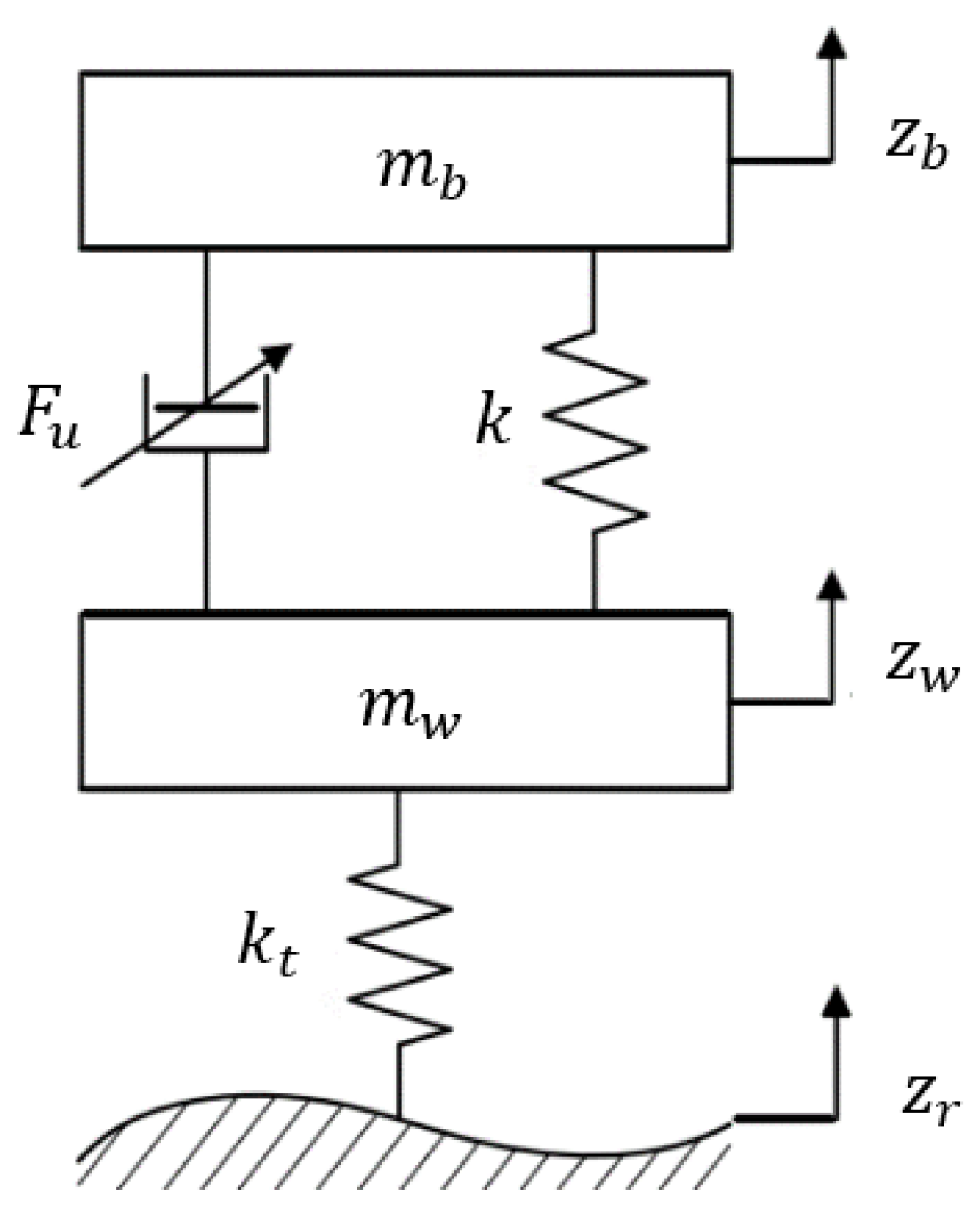
Figure 1 shows the two degree of freedom 1/4 vehicle model.
The two degree of freedom 1/4 vehicle model is widely used to describe the dynamic performance of vehicles. The model can be expressed as follows:
where is the sprung mass acceleration, is the unsprung mass acceleration, is the sprung mass. is the unsprung mass, is the spring stiffness, is the tire stiffness, is the adjustable damping force, is the sprung mass displacement, is the unsprung mass displacement, and is the road elevation.
To simplify the calculation, the two degree of freedom 1/4 vehicle model can be expressed as a state space equation, as follows:
where X is the input variable matrix, Y is the output variable matrix, A, B, C, D and E are the coefficient matrixes, , , and is the road speed.
X and Y can be expressed as follows:
where . . . . . is the sprung mass speed and is the unsprung mass speed.
3. Multiple Fuzzy PID Suspension Control System Based on Road Recognition
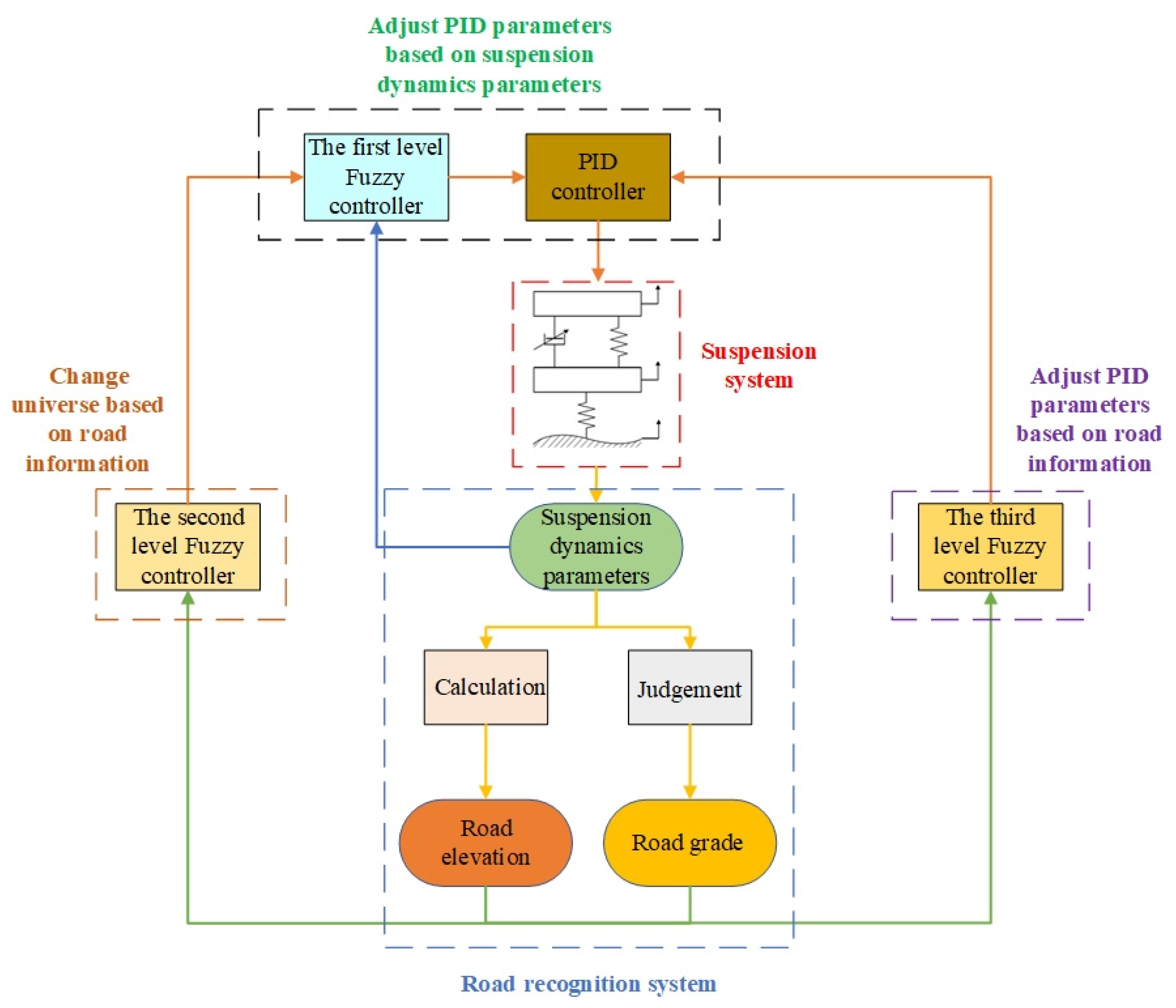
The input of the FPID is the difference between the suspension dynamic parameters and the ideal value, which does not establish a direct relationship between the suspension and road conditions, and ignores the direct effects of the road on the vehicle. The MFRR introduces road recognition technology and adds two fuzzy controllers, based on the FPID. The two fuzzy controllers are the bridge between the road and the first level fuzzy controller and PID controller. The road conditions can be used as control factors to control the dynamic performance of the suspension. The structure of the control system is shown in Figure 2. The road recognition system can carry out road elevation calculations and road grade recognition based on the suspension dynamic parameters. The relevant information calculated according to the road elevation and road grade can be used as the input variables of the second and third level fuzzy controllers.
The second level fuzzy controller establishes a direct relationship between road conditions and the universe expansion factors of the first level fuzzy controller, and its specific principle can be explained as follows:
As shown in Figure 2, the suspension dynamic performance parameters are input into the road recognition system, and the road recognition system calculates the road elevation and road grade according to the input. Then, the difference between the current road elevation and the geometric mean of the root mean square value of the corresponding road elevation of the same grade is calculated. The difference is defined as the relative variation in road displacement, i.e., . and can be expressed as follows:
where i = A, B, C and D, is the geometric mean of the root mean square value of road elevation when road grade is i, and and are the minimum and maximum value of the root mean square value of the road elevation when the road grade is i, respectively.
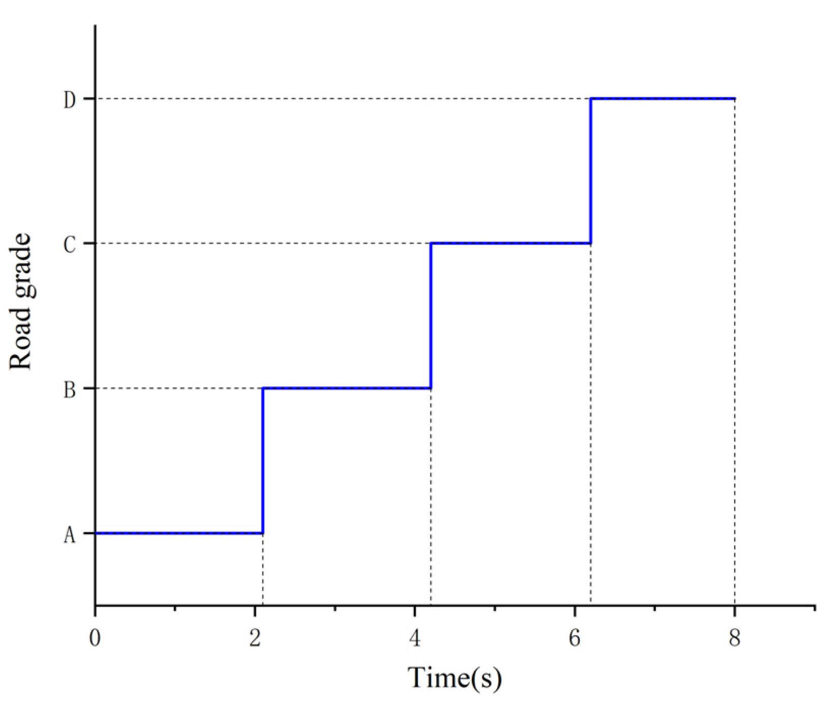
As shown in Figure 3, and the change rate of are the input variables of the second level fuzzy controller. If the relative variation of road displacement is too large, it indicates that the fluctuation of road elevation is relatively large, and if the relative variation of road displacement is small, it indicates that the fluctuation of road elevation is relatively small. The second level fuzzy controller adjusts the universe of the first level fuzzy controller according to the relative variation of road displacement. If the road grade cannot be judged, is the road elevation. Based on the information on road elevation and road grade, the universe expansion factors of the first level fuzzy controller are adjusted in real time based on changes in road conditions, so as to achieve the purpose of the variable universe.
The third level fuzzy controller establishes a direct relationship between road conditions and PID controller control parameters, and its specific principle can be explained as follows:
As shown in Figure 2, the suspension dynamic performance parameters are input into the road recognition system, and the road recognition system calculates the road elevation and road grade according to the input. As shown in Figure 3, and are the input variables of the third level fuzzy controller. If the relative variation of road displacement is too large, it indicates that the fluctuation of road elevation is relatively large, and if the relative variation of road displacement is small, it indicates that the fluctuation of road elevation is relatively small. If the road grade cannot be judged, is the road elevation. The second level fuzzy controller adjusts the control parameters of the PID controller according to the relative variation in road displacement. The third level fuzzy controller establishes a direct relationship between road conditions and the control parameters of the PID controller, and directly adjusts the PID parameters based on the road elevation and road grade information. Based on the adjustment of the control parameters of the PID controller by the first level fuzzy controller, the secondary adjustment of control parameters of the PID controller can be carried out.
4. Road Recognition
4.1. Road Elevation Calculation
As road elevation is not easy to measure directly, it is derived inversely based on vehicle dynamic performance in this paper. Road fluctuation directly acts on the tire and causes tire vibration, so there is a direct relationship between tire acceleration and road elevation. The road elevation can be inversely derived from the unsprung mass acceleration.
The variable damping force can be expressed as:
where is the damping coefficient.
Therefore, Equation (8) can be expressed as follows:
A Laplace transformation is performed on Equation (8), and can be expressed as follows:
The unsprung mass acceleration is selected as the input signal, which can be expressed as follows:
The transfer relationship between the unsprung mass acceleration and the road elevation can be expressed as follows:
Equation (11) can be simplified as follows:
where , , , , , , , , , .
The inverse derivation model of road elevation can be expressed as:
According to Equation (13), the road elevation can be calculated by measuring the unsprung mass acceleration.
4.2. Road Grade Recognition
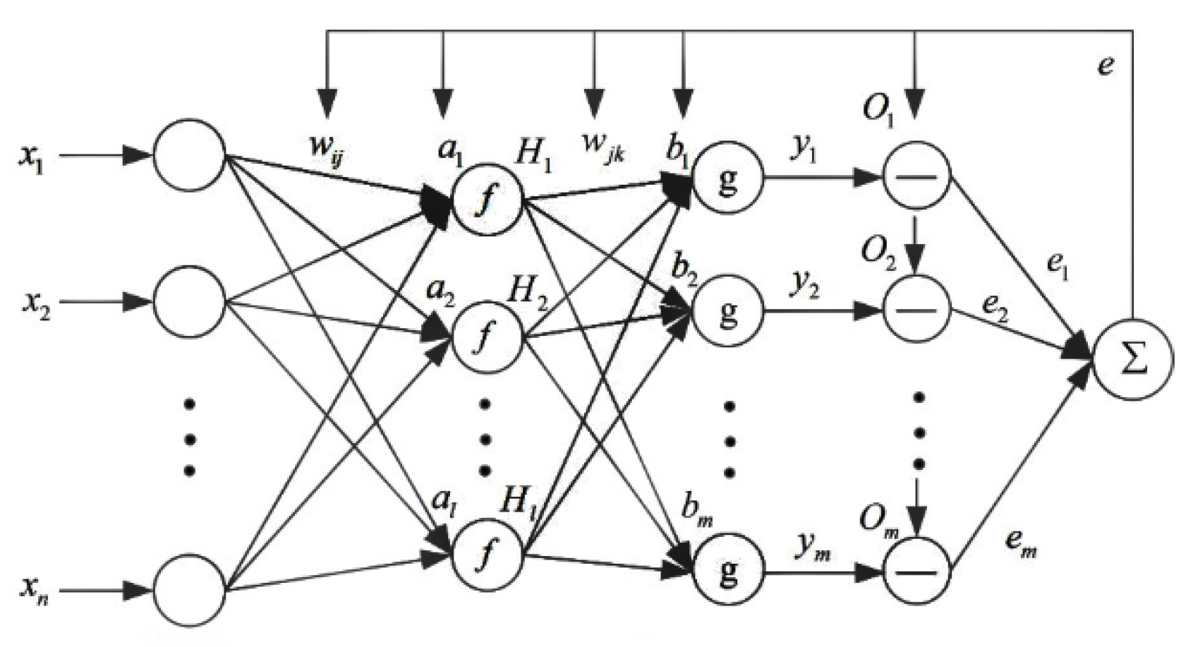
In this paper, a BP neural network algorithm was used for road grade recognition. The structure of the BP neural network is shown in Figure 6. A BP neural network is a learning and training process in which the error propagates backward and modifies the weight coefficient at the same time. Using the gradient steepest descent method, following the principle of minimizing the total error of the network, the weight is continuously adjusted to minimize the root mean square error between the actual output value and the expected output value of the network.
When the vehicle is running normally, the road excitation will directly act on the wheels, causing wheel vibration, which directly determines the unsprung mass acceleration. The road excitation will indirectly act on the sprung mass through the suspension, causing the sprung mass vibration—thus affecting the sprung mass acceleration. On the same grade of road, with an increase in vehicle speed, both unsprung mass acceleration and sprung mass acceleration will change greatly. There is an obvious corresponding relationship between the three parameters. As such, the unsprung mass acceleration, sprung mass acceleration, and vehicle speed were selected as the basis of road grade recognition, and set as the input layer nodes. Grade A, B, C and D roads were selected as the output layer nodes. Based on previous experience, the number of hidden layers was set to two, and the number of hidden layer nodes was set to four and eight. Therefore, the structure of the road recognition neural network model was [3 4 8 4].
The activation function logsig from the input layer to the first hidden layer could be determined by the trial method, which can be expressed as follows:
The activation function Tansig from the first hidden layer to the second hidden layer can be expressed as follows:
The activation function purelin from the second hidden layer to the output layer can be expressed as:
The sample input and output data were trained, and the prediction probability of road grade was:
where and are the connection weight and threshold from the input layer to the first hidden layer, and are the connection weight and threshold from the first hidden layer to the second hidden layer, and and are the connection weight and threshold from the second hidden layer to the third hidden layer.
The two degree of freedom 1/4 vehicle model was built in Matlab/Simulink to simulate the unsprung mass acceleration and unsprung mass displacement under different road grades, and the training sample data were obtained. The Levenberg–Marquardt algorithm was adopted; the learning rate was set to 0.005, the input and output data were trained, and the probability of each road grade corresponding to the input data was calculated by the neural network model. The road grade corresponding to the maximum probability was the final output, so as to complete the recognition of road grade.
5. Controller Design
5.1. Design of the Second Level Fuzzy Controller
The second level fuzzy controller adopted the form of two inputs and three outputs; and were the input variables. The fuzzy subset of input variables was , and the universe was . As shown in Figure 3, expansion factors and of the input variables universe of the first level fuzzy controller, and the expansion factor β of the output variables universe of the first level fuzzy controller, were the output variables of the second level fuzzy controller. The fuzzy subset of the output variables was , and the universe was . The fuzzy rules of the second level fuzzy controller are shown in Table 1.
The control rules of expansion factors were as follows:
- (1)
- When and were large, in order to ensure that the system had small error and a fast dynamic response, the universe of input variables were appropriately increased and the universe of output variables were kept unchanged.
- (2)
- When and were small, in order to avoid a large overshoot of the system, the universes of input and output variables were appropriately reduced.
In this paper, a triangular membership function and centroid defuzzification method were used.
5.2. Design of the Third Level Fuzzy Controller
The third level fuzzy controller adopted the form of two inputs and three outputs. and were the input variables. The fuzzy subset of input variables was , and the universe was . As shown in Figure 3, the output variables were the secondary adjustments , and of the control parameters , and of the PID controller. The fuzzy subset of input variables was , and the universe was . The fuzzy rules of the third level fuzzy controller are shown in Table 2.
The adjustment rules of , and were as follows:
- (1)
- When was large, in order to improve the response speed of the system and ensure that the suspension system was within the controllable range, was appropriately increased.
- (2)
- When and were basically equal and of moderate size, in order to reduce the system overshoot and improve the response speed, was reduced, and and were appropriately reduced.
- (3)
- When was small, and was increased. varies depending on . When was small, was increased appropriately. When was large, was kept unchanged to reduce system overshoot and ensure system stability.
5.3. Design of the First Level Fuzzy Controller
The first level fuzzy controller adopted the form of two inputs and three outputs. As shown in Figure 3, the difference between the sprung mass acceleration and the expected value and its change rate were input variables, which are represented by error signal e and error signal change rate ec, respectively. The fuzzy subset of input variables was , and the universe was . The output variables were the primary adjustments , and of the control parameters , and of the PID controller. The fuzzy subset of input variables was , and the universe was . In this paper, a triangular membership function and centroid defuzzification method were used. The fuzzy rules of the first level fuzzy controller are shown in Table 3.
The initial control parameters , and of the PID controller were adjusted by the two level controller to obtain the final control parameters , and . They can be expressed as follows:
Therefore, the adjustable damping force of semi-active suspension can be expressed as:
Figure 9 is a flow chart of MFRR. In short, if the suspension dynamic performance meets expectations, the damping force will not be adjusted. If the suspension dynamic performance does not meet expectations, each control system will adjust the damping force according to the input in order to achieve a suspension dynamic performance that meets expectations.
MFRR can calculate road elevation in real time, and carry out road grade recognition based on the road elevation data, and further optimize the controller parameters. Compared with the existing control system, MFRR makes up for the deficiency of the existing control system in which it cannot collect and use road data to adjust the suspension performance. MFRR has multiple fuzzy controllers, and there are many types of fuzzy controller input variables. MFRR can adjust the control effect in real time based on multiple pieces of information. Compared with the existing control system, it solves the problems of having too many single input parameters and the low control performance of the existing control system.
6. Road Model
6.1. Road of Each Grade
The road power spectral density can be expressed as follows:
where n is the spatial frequency, n0 is the reference spatial frequency, is the power spectral density of the road profiles, and W is the frequency index.
The time frequency f is:
where v is the vehicle speed.
Equation (20) can be expressed as follows:
can be expressed as follows:
where is the cut-off frequency.
The transfer function can be expressed as follows:
Then, the road elevation can be expressed as:
where is the lower cut-off frequency, and is white noise.
The road excitation of each grade can be constructed according to Equation (26).
6.2. Single Bump Road
A single-bump road can be expressed as follows:
where h is the signal amplitude, and l is the signal length. In this paper, h = 0.1 m and l = 0.25 m were selected.
6.3. Sinusoidal Road
A sinusoidal road with an amplitude of 0.1 m and frequency of 3 Hz was selected. A sinusoidal road can be expressed as follows:
A summary of various roads is shown in Figure 10.
7. Experimental Analysis
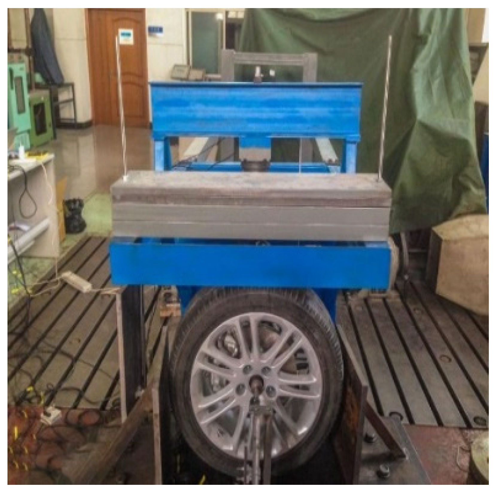
The quarter suspension test bench used in the experiment is shown in the Figure 11. Parameters of the vehicle are shown in Table 4.
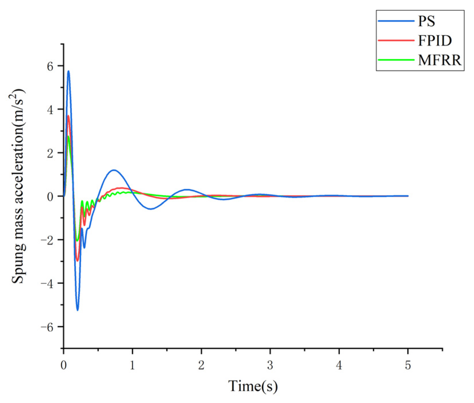
The results of the single bump road input are shown in Figure 12. The SMA of the MFRR was obviously less than that of the other two control systems, and the acceleration attenuation speed was faster. The root mean square value of the SMA of the three systems and its reduction relative to the PS under the input of single bump road are shown in Table 5. As shown in the table, the SMA of FPID was reduced by 22.49%, and the SMA of MFRR was reduced by 38.47%.
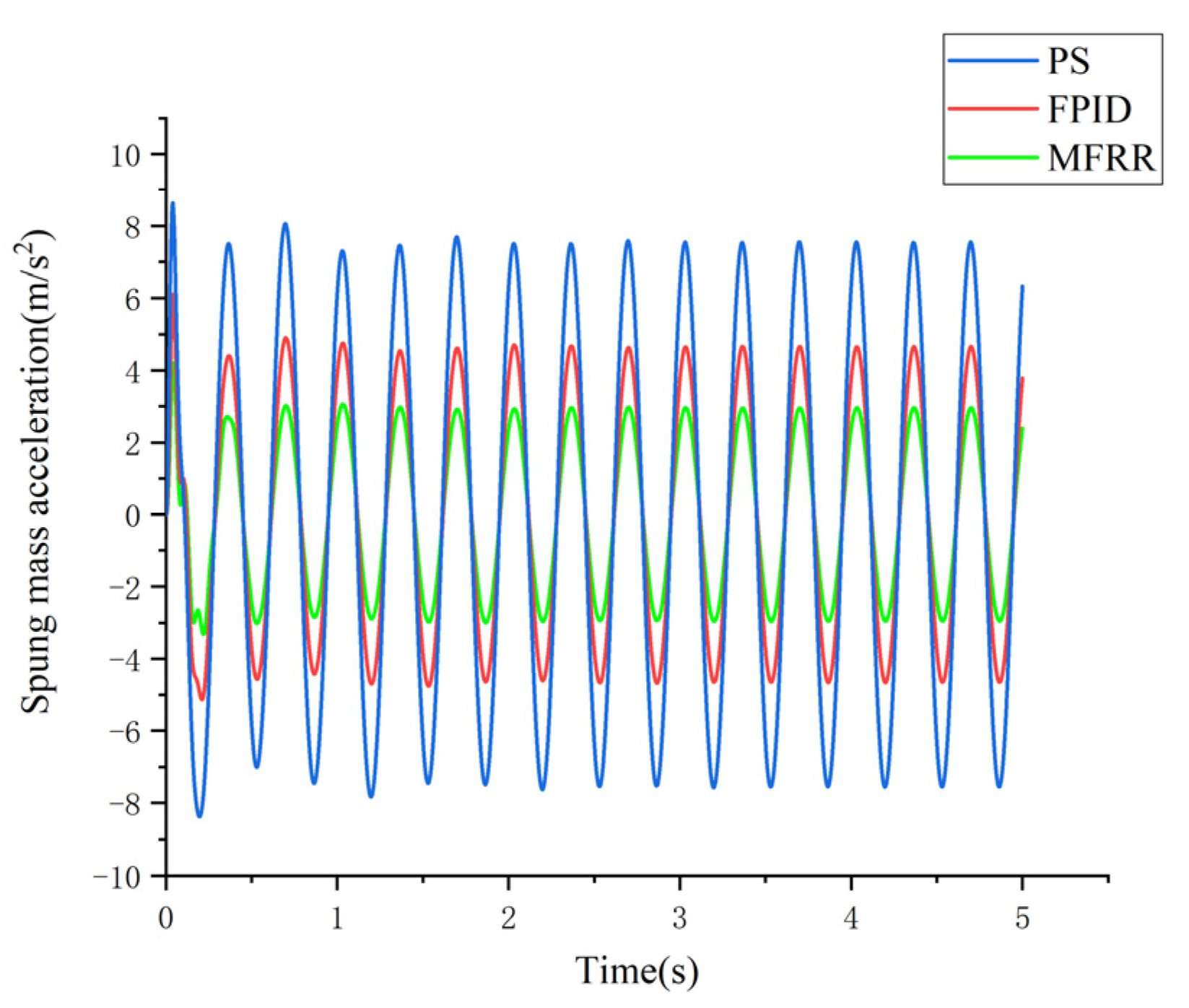
The results of the sinusoidal road input are shown in Figure 13. The SMA of MFRR was obviously smaller than that of the other two systems. The root mean square value of the SMA of the three systems and its reduction relative to the PS are shown in the Table 6. Compared with the PS, the SMA of the FPID was reduced by 60.90%, and the SMA of MFRR was reduced by 71.29%.
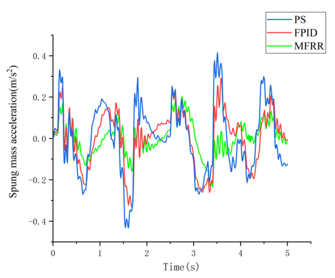
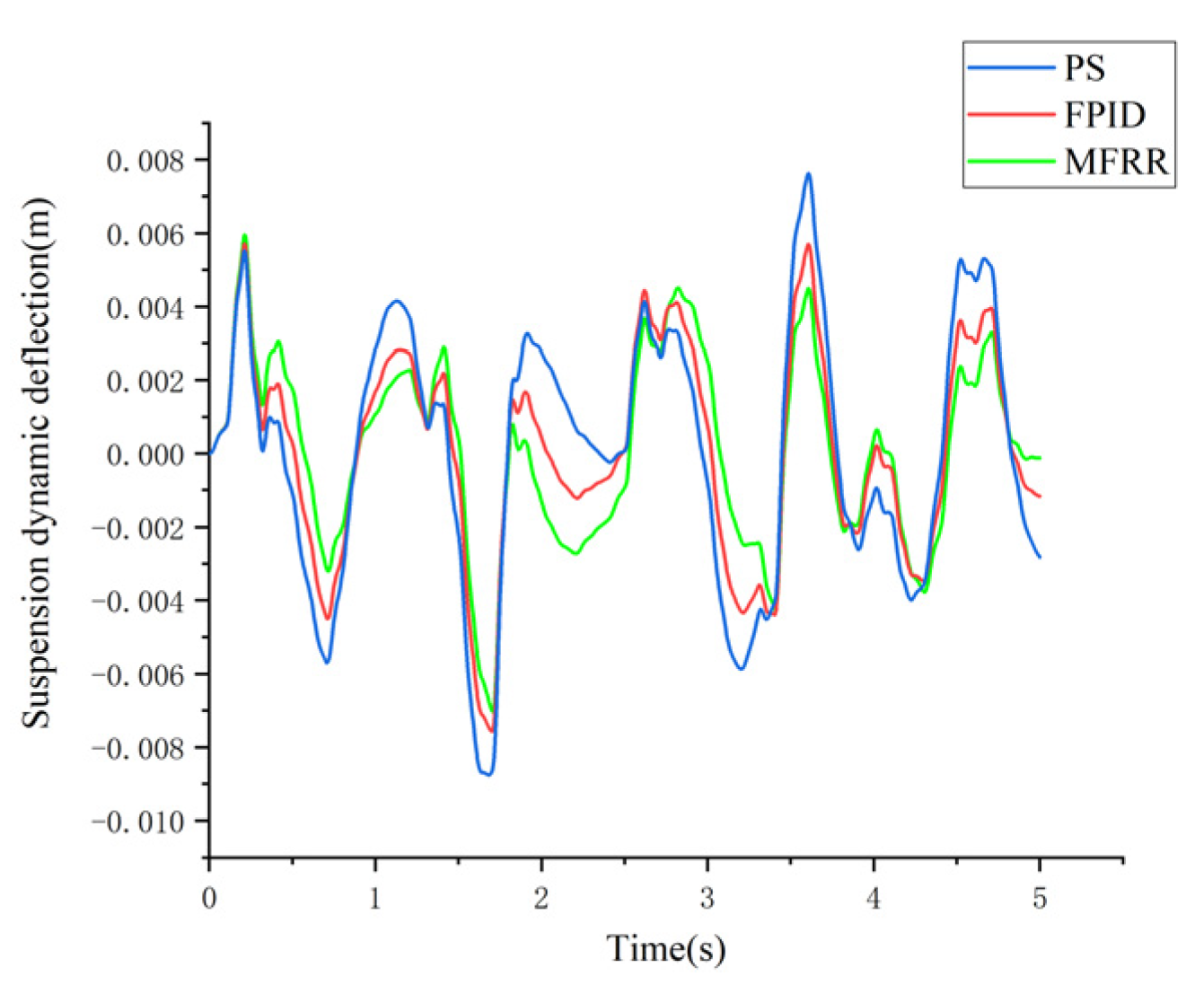
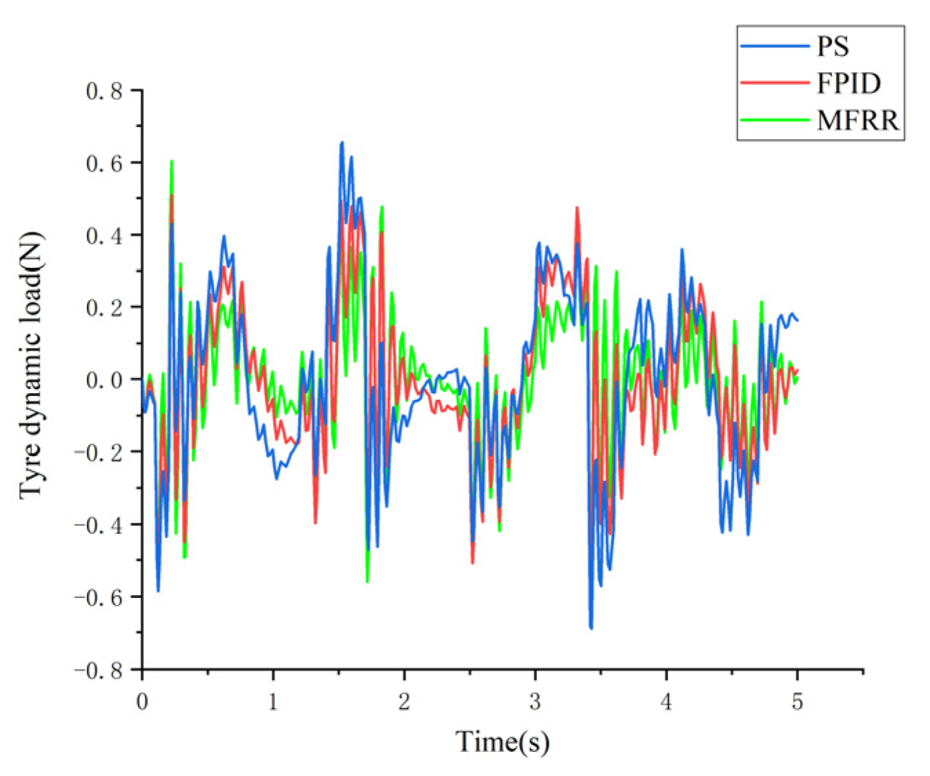
The results of SMA, SDD and TDL under grade B road input are shown in Figure 14, Figure 15 and Figure 16. The SMA, SDD and TDL of MFRR were significantly less than the other two systems.
The results of the three systems on various grades of roads are shown in Table 7, and the reduction of dynamic parameters relative to PS is shown in Table 8. The root mean square values of SMA, SDD and TDL of the MFRR were significantly reduced. Taking grade B road as an example, compared with PS, the reductions in SMA, SDD and TDL in the FPID were 21.56%, 20.00% and 14.96% respectively. The reductions in SMA, SDD and TDL in the MFRR were 40.01%, 34.28% and 32.64% respectively. The MFRR had better control performance than the FPID.
8. Conclusions
Based on the FPID controller, the MFRR was designed. The control system can adjust the control parameters of the controller in real time according to changes in road conditions. A two degree of freedom 1/4 vehicle model was established, and a mathematical model of suspension was established based on this model, and the control rules of each controller were designed, respectively. The control performance of three suspension systems was analyzed through experiments. The test results showed that:
- (1)
- Compared with the PS, with the single-bump road input, the SMA of the FPID was reduced by 22.49%, and the SMA of the MFRR was reduced by 38.47%.
- (2)
- Compared with the PS, with the sinusoidal road input, the SMA of the FPID was reduced by 60.90%, and the SMA of the MFRR was reduced by 71.29%.
- (3)
- Taking grade B road as an example, compared with the PS, the reductions in the SMA, SDD and TDL of the FPID were 21.56%, 20.00% and 14.96%, respectively. The reductions in the SMA, SDD and TDL of the MFRR were 40.01%, 34.28% and 32.64%, respectively.
Compared with the PS and FPID, the MFRR had a better dynamic performance.
This research was based on the two degree of freedom 1/4 vehicle model, with no further verification or analysis of the whole vehicle model. The fuzzy control rules were designed based on previous experience and are subject to a certain degree of subjectivity. Next, an analysis of whole vehicle dynamic performance and optimization of fuzzy control rules will be our focus.
9. Patents
Ruichuan Li, Xinkai Ding, Huilai Sun, et al. Enhanced multiple fuzzy PID control system and method for semi-active suspension: China, CN202110274785.1. 2021-03-15.
Author Contributions
Conceptualization, X.D. and R.L.; methodology, X.D.; software, X.D.; validation, R.L., Y.C. and Q.L.; formal analysis, X.D.; investigation, Y.C.; resources, R.L.; data curation, J.L.; writing—original draft preparation, X.D.; writing—review and editing, X.D.; visualization, J.L.; supervision, Q.L.; project administration, R.L.; funding acquisition, R.L. All authors have read and agreed to the published version of the manuscript.
Funding
1. Industrial foundation strengthening project of the Ministry of industry and information technology of the people’s Republic of China, grant number TC180A3Y1; 2. National key R & D projects, grant number 2016YFD0701104; 3. Major innovation projects in Shandong Province, China, grant number 2019TSLH0303; 4. Key R&D plan of Shandong Province, China, grant number 2020CXGC010806; 5. Key R&D plan of Shandong Province, China, grant number 2020CXGC011005; 6. Innovation team project of colleges and universities of Jinan science and Technology Bureau, Shandong Province, China, grant number 2020GXRC042.
Institutional Review Board Statement
Not applicable.
Informed Consent Statement
Not applicable.
Data Availability Statement
The data presented in this study are available on request from the corresponding author.
Acknowledgments
I would like to thank my tutor, Ruichuan Li, for all his support and guidance. I would like to thank my colleagues for their care and help in my daily work.
Conflicts of Interest
The authors declare no conflict of interest.
References
- Cao, D.P.; Song, X.B.; Ahmadian, M. Road vehicle suspension design, dynamics, and control. Vehicle Syst. Dyn. 2011, 49, 3–28. [Google Scholar] [CrossRef] [Green Version]
- Nakano, K.; Suda, Y.; Yamaguchi, M.; Kohno, H. Application of combined type self powered active suspensions to rubber-tired vehicles. JSAE Meet. 2003, 6, 19–22. [Google Scholar] [CrossRef]
- Crews, J.H.; Mattson, M.G.; Buckner, G.D. Multi-objective control optimization for semi-active vehicle suspensions. J. Sound Vib. 2011, 330, 5502–5516. [Google Scholar] [CrossRef]
- Qin, Y.; Xiang, C.; Wang, Z.; Dong, M.M. Road excitation classification for semi-active suspension system based on system response. J. Vib. Control 2018, 24, 2732–2748. [Google Scholar] [CrossRef]
- Jagga, D.; Lv, M.; Baldi, S. Hybrid Adaptive Chassis Control for Vehicle Lateral Stability in the Presence of Uncertainty. In Proceedings of the 2018 26th Mediterranean Conference on Control and Automation (MED), Zadar, Croatia, 19–22 June 2018; pp. 1–6. [Google Scholar]
- Majdoub, K.E.; Giri, F.; Chaoui, F.Z. Adaptive Backstepping Control Design for Semi-Active Suspension of Half-Vehicle With Magnetorheological Damper. IEEE/CAA J. Autom. Sin. 2021, 8, 582–596. [Google Scholar] [CrossRef]
- Precup, R.E.; Preitl, S.; Petriu, E.; Bojan-Dragos, C.A.; Szedlak-Stinean, A.I.; Roman, R.C.; Hedrea, E.L. Model-Based Fuzzy Control Results for Networked Control Systems. Rep. Mech. Eng. 2020, 1, 10–25. [Google Scholar] [CrossRef]
- Gharib, M.R. Comparison of robust optimal QFT controller with TFC and MFC controller in a multi-input multi-output system. Rep. Mech. Eng. 2020, 1, 151–161. [Google Scholar] [CrossRef]
- Xu, L.; Cao, Q.S.; Zhang, D.Y. Fractional order control strategy of active suspension based on QPSO. J. Vib. Shock 2021, 40, 227–233. [Google Scholar]
- Li, G.; Gu, R.H.; Xu, R.X.; Hu, G.L.; Ouyang, N.; Xu, M. Study on Fuzzy LQG Control Strategy for Semi-active Vehicle Suspensions with Magnetorheological Dampers. Noise Vib. Control 2021, 41, 129–136. [Google Scholar] [CrossRef]
- Huang, Y.B.; Lü, Y.F.; Zhao, G.; Na, J.; Zhao, J. Adaptive Optimal Control for Nonlinear Active Suspension Systems. Control Decis. 2021, 8, 1–9. [Google Scholar]
- Al Aela, A.M.; Kenne, J.-P.; Angue Mintsa, H. A Novel Adaptive and Nonlinear Electrohydraulic Active Suspension Control System with Zero Dynamic Tire Liftoff. Machines 2020, 8, 38. [Google Scholar] [CrossRef]
- Liu, Y.J.; Chen, H. Adaptive Sliding Mode Control for Uncertain Active Suspension Systems With Prescribed Performance. IEEE Trans. Syst. Man Cybern. Syst. 2021, 51, 6414–6422. [Google Scholar] [CrossRef]
- Min, X.; Li, Y.M.; Tong, S.C. Adaptive fuzzy output feedback inverse optimal control for vehicle active suspension systems. Neurocomputing 2020, 403, 257–267. [Google Scholar] [CrossRef]
- Wang, G.; Chadli, M.; Basin, M.V. Practical Terminal Sliding Mode Control of Nonlinear Uncertain Active Suspension Systems with Adaptive Disturbance Observer. IEEE/ASME Trans. Mech. 2021, 26, 789–797. [Google Scholar] [CrossRef]
- Mohammadikia, R.; Aliasghary, M. Design of an interval type-2 fractional order fuzzy controller for a tractor active suspension system. Comput. Electron. Agric. 2019, 167, 105049. [Google Scholar] [CrossRef]
- Pang, H.; Liu, F.; Xu, Z.R. Variable universe fuzzy control for vehicle semi-active suspension system with MR damper combining fuzzy neural network and particle swarm optimization. Neurocomputing 2018, 306, 130–140. [Google Scholar] [CrossRef]
- Singh, D. Modeling and control of passenger body vibrations in active quarter car system: A hybrid ANFIS PID approach. Int. J. Dyn. Control 2018, 6, 1649–1662. [Google Scholar] [CrossRef]
- Nugroho, P.W.; Li, W.; Du, H.; Alici, G.; Yang, J. An adaptive neuro fuzzy hybrid control strategy for a semiactive suspension with magneto rheological damper. Adv. Mech. Eng. 2014, 6, 487312. [Google Scholar] [CrossRef]
- Tang, X.; Du, H.; Sun, S. Takagi–Sugeno fuzzy control for semi-active vehicle suspension with a magnetorheological damper and experimental validation. IEEE Trans. Mechatron. 2017, 22, 291–300. [Google Scholar] [CrossRef]
- Devdutt, M.L. Fuzzy logic control of a semi-active quarter car system. Int. J. Mech. Ind. Sci. Eng. 2014, 8, 163–167. [Google Scholar]
- Khodadadi, H.; Ghadiri, H. Self-tuning PID controller design using fuzzy logic for half car active suspension system. Int. J. Dyn. Control 2018, 6, 224–232. [Google Scholar] [CrossRef]
- Swethamarai, P.; Lakshmi, P. Adaptive-fuzzy fractional order pid controller-based active suspension for vibration control. IETE J. Res. 2020, 1–16. [Google Scholar] [CrossRef]
- Kumar, V.; Ran, K.P.S.; Kumar, J.; Mishra, P. Self-tuned robust fractional order fuzzy PD controller for uncertain and nonlinear active suspension system. Neural Comput. Appl. 2018, 30, 1827–1843. [Google Scholar] [CrossRef]
- Gad, S.; Metered, H.; Bassuiny, A.; Ghany, A.A. Multi-objective genetic algorithm fractional-order PID controller for semi-active magneto rheologically damped seat suspension. J. Vib. Control 2017, 23, 1248–1266. [Google Scholar] [CrossRef]
- Nagarkar, M.P.; Bhalerao, Y.J.; Vikhe, P.G.J.; Patil, R.N.Z. GA-based multi-objective optimization of active nonlinear quarter car suspension system—PID and fuzzy logic control. Int. J. Mech. Mater. Eng. 2018, 13, 10. [Google Scholar] [CrossRef]
Figure 1.
Two degree of freedom 1/4 vehicle model.

Figure 2.
Control system structure.

Figure 3.
Control system principle. r is the ideal input. y is the control signal, e is the error signal, ec is the rate of change of the error signal, and are the expansion factors of the input variable universe, is the expansion factors of the output variable universe, , and are the primary adjustments of the control parameters of the PID controller, and , and are the secondary adjustments of the control parameters of the PID controller.

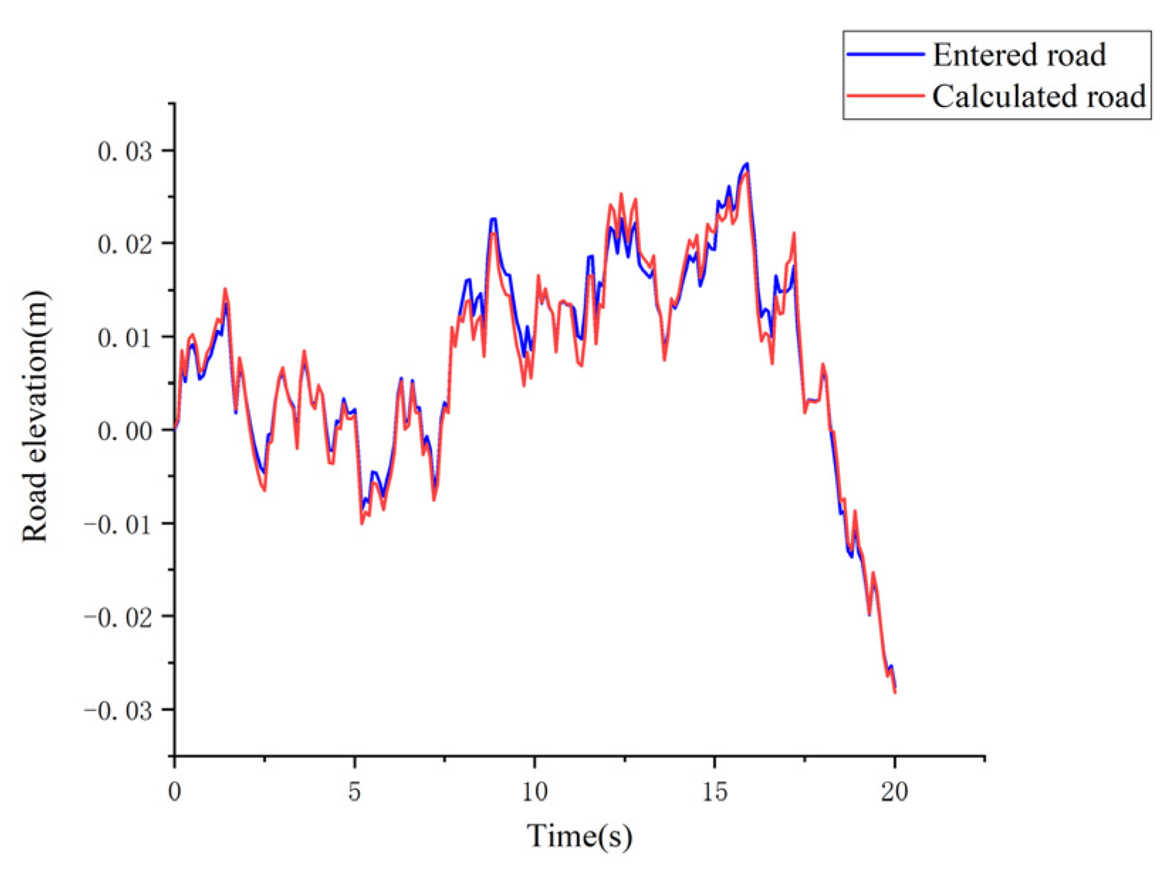
Figure 4.
Grade B road.

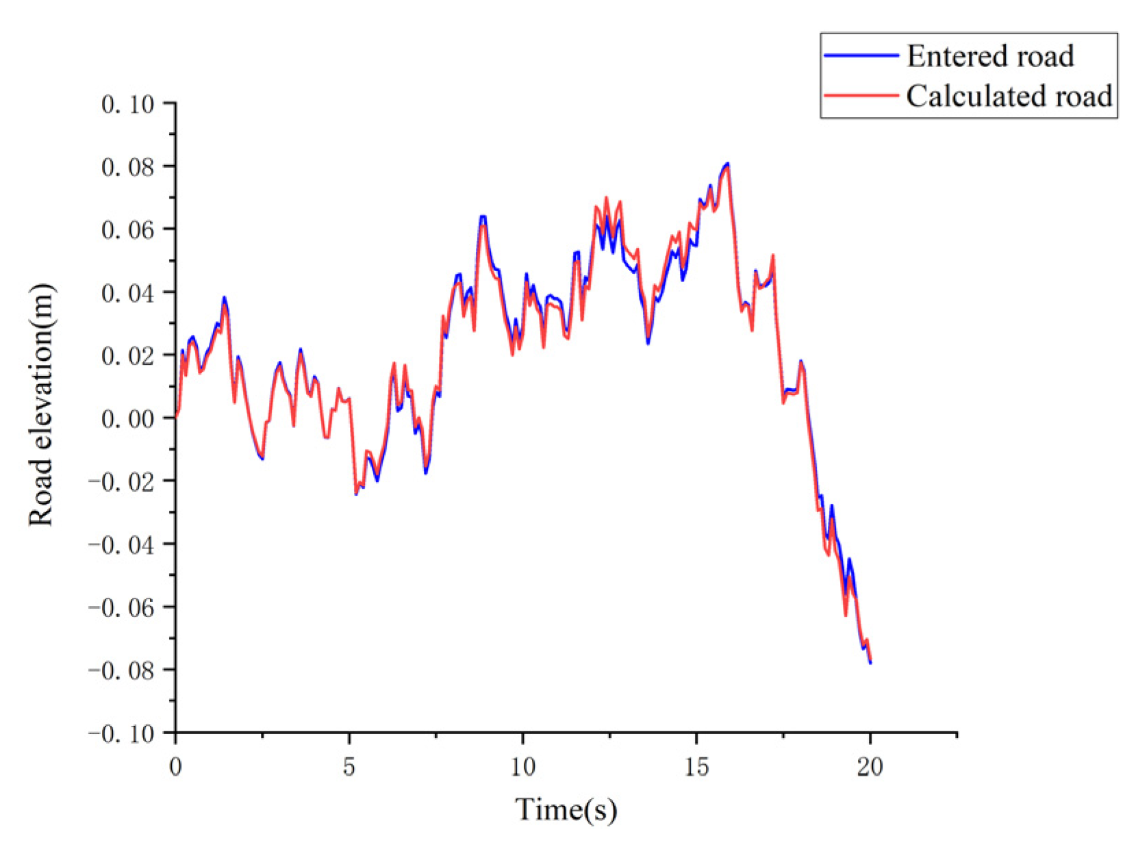
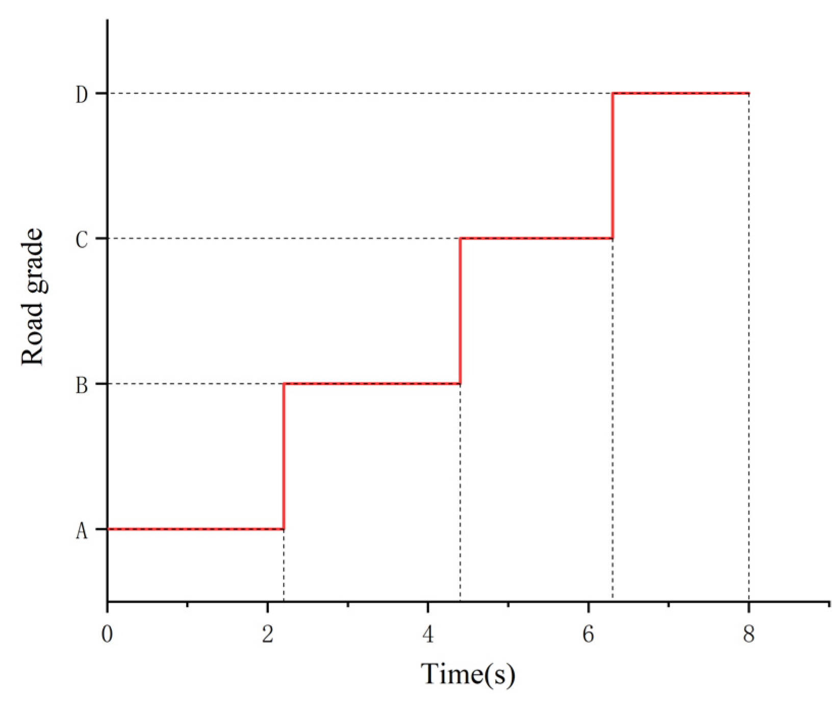
Figure 5.
Grade C road.

Figure 6.
The structure of the BP neural network.

Figure 7.
30 km/h.

Figure 8.
50 km/h.

Figure 9.
Flowchart of MFRR.

Figure 10.
Road summary.

Figure 11.
Test bench.

Figure 12.
The SMA.

Figure 13.
SMA.

Figure 14.
SMA.

Figure 15.
SDD.

Figure 16.
TDL.


Table 1.
The fuzzy rules of the second level fuzzy controller.
| NB | NM | NS | ZO | PS | PM | PB | |
|---|---|---|---|---|---|---|---|
| NB | PB/PB/PB | PB/PB/PM | PM/PM/PS | PS/PM/ZO | PM/PM/PS | PB/PB/PM | PB/PB/PB |
| NM | PB/PB/PB | PM/PB/PB | PS/PS/PM | PS/PS/PS | PS/PS/PM | PM/PB/PB | PB/PB/PB |
| NS | PM/PM/PB | PM/PM/PS | PS/PS/PS | ZO/ZO/PS | ZO/ZO/PS | PM/PM/PM | PM/PM/PB |
| ZO | PM/PM/PM | PS/PS/PM | ZO/ZO/PS | ZO/ZO/ZO | ZO/ZO/ZO | PS/PS/PM | PM/PM/PM |
| PS | PM/PM/PM | PM/PM/PS | PS/PS/ZO | ZO/ZO/ZO | PS/PS/ZO | PM/PM/PS | PM/PM/PM |
| PM | PB/PB/PM | PM/PB/PM | PS/PS/PS | PS/PS/ZO | PS/PS/PS | PM/PB/PM | PB/PB/PM |
| PB | PB/PB/PB | PB/PB/PM | PM/PM/PS | PS/PM/PS | PM/PM/PS | PB/PB/PM | PB/PB/PB |
Table 2.
The fuzzy rules of the third level fuzzy controller.
| NB | NM | NS | ZO | PS | PM | PB | |
|---|---|---|---|---|---|---|---|
| NB | PB/NB/PS | PB/NB/NS | PM/NM/NB | PM/PM/NB | NS/NS/NB | ZO/ZO/NM | ZO/ZO/PS |
| NM | PB/NB/PS | PB/NB/NS | PM/NM/NB | PS/PS/NM | NS/NS/NM | ZO/ZO/NS | NS/ZO/ZO |
| NS | PM/NM/ZO | PM/NM/NS | PM/NS/NM | PS/PS/NM | ZO/ZO/NS | NS/PS/NS | NS/PS/ZO |
| ZO | PM/NM/ZO | PM/NM/NS | PS/NS/NS | ZO/ZO/NS | PS/PS/NS | NM/PM/NS | NM/PM/ZO |
| PS | PS/NM/ZO | PS/NS/ZO | ZO/ZO/ZO | NS/PS/ZO | PS/PS/ZO | NM/PM/ZO | NM/PB/ZO |
| PM | PS/ZO/PB | ZO/ZO/NS | NS/PS/PS | NM/PS/PS | PM/PM/PS | NM/PB/PS | NB/PB/PB |
| PB | ZO/ZO/PB | ZO/ZO/PM | NM/PS/PM | NM/PM/PM | PM/PM/PS | NB/PB/PS | NB/PB/PB |
Table 3.
The fuzzy rules of the first level fuzzy controller.
| e | ec | ||||||
|---|---|---|---|---|---|---|---|
| NB | NM | NS | ZO | PS | PM | PB | |
| NB | ZO/PS/PS | PB/ZO/NM | PM/PB/NS | PB/PM/NB | PS/NS/NB | NS/NS/NM | PB/PM/NS |
| NM | ZO/NM/NM | NM/NM/PS | NS/NS/ZO | PM/PS/NM | ZO/PM/NS | PM/ZO/PM | PB/ZO/PM |
| NS | PB/NM/NM | ZO/NB/PM | PM/NS/NM | NB/NM/PM | NS/NS/PB | NS/PS/NS | PM/PB/NS |
| ZO | ZO/PS/PM | PM/NM/NS | ZO/NS/NM | ZO/NM/NS | ZO/NS/PB | PM/NS/NM | NB/NM/ZO |
| PS | PM/PM/ZO | NM/NS/NM | ZO/PM/PM | NM/ZO/PM | ZO/PS/NB | PM/NB/NB | NM/NB/ZO |
| PM | PS/NM/PB | NM/ZO/PS | PB/NS/PB | NB/PM/NM | NB/PM/PM | PB/PM/NS | NM/PS/NS |
| PB | ZO/PS/NS | PB/NB/PM | PS/PM/PM | PB/NM/PM | PM/PS/PM | NM/PM/NM | PB/ZO/PM |
Table 4.
Parameters of the vehicle.
| Parameters | Values |
|---|---|
| Sprung mass (mb) | 230 kg |
| Unsprung mass (mw) | 40 kg |
| Spring stiffness (k) | 15,026 N/m |
| Tire Stiffness (kt) | 196,400 N/m |
Table 5.
Root mean square value and reduction of SMA.
| Control System | SMA(m/s2) | Reduction of SMA(%) |
|---|---|---|
| PS | 1.3882 | / |
| FPID | 1.0760 | 22.49 |
| MFRR | 0.8542 | 38.47 |
Table 6.
Root mean square value and reduction of SMA.
| Control System | SMA(m/s2) | Reduction of SMA(%) |
|---|---|---|
| PS | 5.3375 | / |
| FPID | 2.0871 | 60.90 |
| MFRR | 1.5324 | 71.29 |
Table 7.
The results of the three systems on various grades of roads.
| Road Grade | Control System | SMA(m/s2) | SDD(m) | TDL(N) |
|---|---|---|---|---|
| A | PS | 0.0926 | 0.0019 | 0.1326 |
| FPID | 0.0727 | 0.0016 | 0.1119 | |
| MFRR | 0.0581 | 0.0011 | 0.9860 | |
| B | PS | 0.1702 | 0.0035 | 0.2454 |
| FPID | 0.1335 | 0.0028 | 0.2087 | |
| MFRR | 0.1021 | 0.0023 | 0.1653 | |
| C | PS | 0.3148 | 0.0064 | 0.4479 |
| FPID | 0.2437 | 0.0053 | 0.3792 | |
| MFRR | 0.1961 | 0.0044 | 0.3112 | |
| D | PS | 0.5550 | 0.0113 | 0.8035 |
| FPID | 0.4359 | 0.0091 | 0.6791 | |
| MFRR | 0.3517 | 0.0081 | 0.5725 |
Table 8.
The reduction of the three systems on various grades of roads.
| Road Grade | Control System | Reduction of SMA(%) | Reduction of SDD(%) | Reduction of TDL(%) |
|---|---|---|---|---|
| A | PS | / | / | / |
| FPID | 21.49 | 15.79 | 15.61 | |
| MFRR | 37.26 | 26.32 | 25.64 | |
| B | PS | / | / | / |
| FPID | 21.56 | 20.00 | 14.96 | |
| MFRR | 40.01 | 34.28 | 32.64 | |
| C | PS | / | / | / |
| FPID | 22.59 | 17.19 | 15.34 | |
| MFRR | 37.71 | 31.25 | 30.52 | |
| D | PS | / | / | / |
| FPID | 21.46 | 19.47 | 15.48 | |
| MFRR | 36.63 | 28.31 | 28.75 |
Publisher’s Note: MDPI stays neutral with regard to jurisdictional claims in published maps and institutional affiliations. |
© 2021 by the authors. Licensee MDPI, Basel, Switzerland. This article is an open access article distributed under the terms and conditions of the Creative Commons Attribution (CC BY) license (https://creativecommons.org/licenses/by/4.0/).
Share and Cite
MDPI and ACS Style
Ding, X.; Li, R.; Cheng, Y.; Liu, Q.; Liu, J. Design of and Research into a Multiple-Fuzzy PID Suspension Control System Based on Road Recognition. Processes 2021, 9, 2190. https://0-doi-org.brum.beds.ac.uk/10.3390/pr9122190
AMA Style
Ding X, Li R, Cheng Y, Liu Q, Liu J. Design of and Research into a Multiple-Fuzzy PID Suspension Control System Based on Road Recognition. Processes. 2021; 9(12):2190. https://0-doi-org.brum.beds.ac.uk/10.3390/pr9122190
Chicago/Turabian StyleDing, Xinkai, Ruichuan Li, Yi Cheng, Qi Liu, and Jilu Liu. 2021. "Design of and Research into a Multiple-Fuzzy PID Suspension Control System Based on Road Recognition" Processes 9, no. 12: 2190. https://0-doi-org.brum.beds.ac.uk/10.3390/pr9122190
Note that from the first issue of 2016, this journal uses article numbers instead of page numbers. See further details here.