Optimal Sensor Placement in a Partitioned Water Distribution Network for the Water Protection from Contamination †

 , , and
Abstract
:1. Introduction
2. Materials and Methods
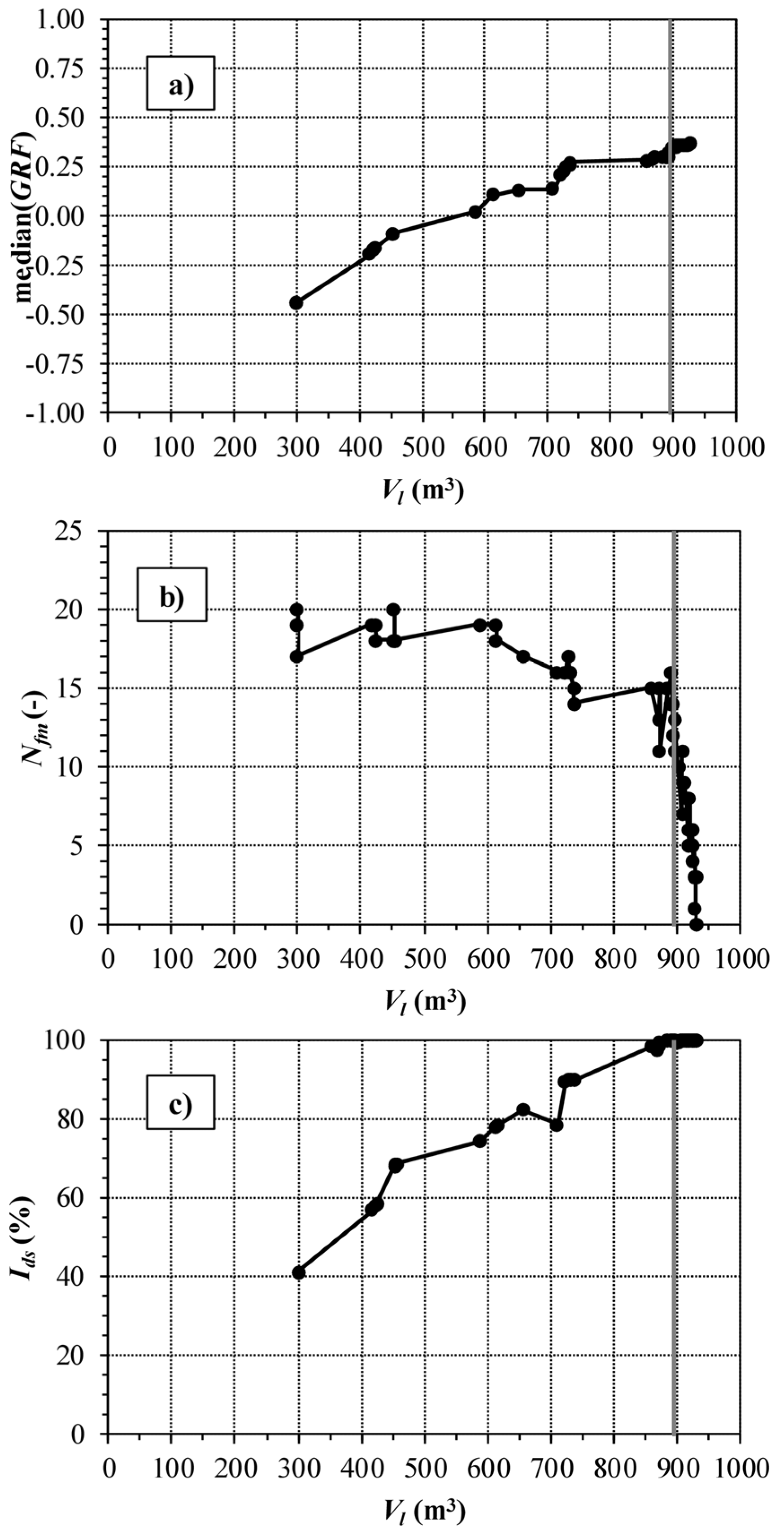
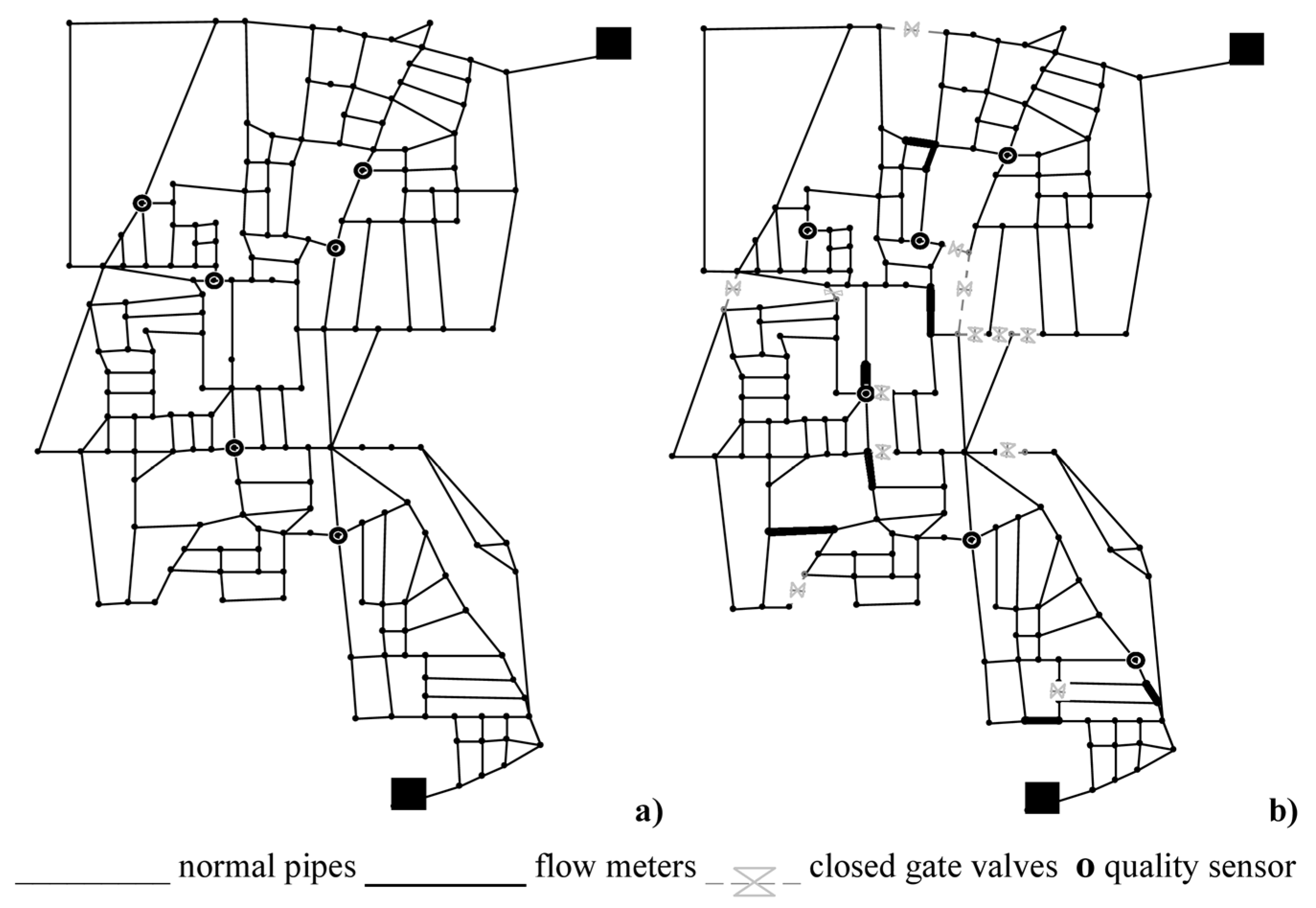
2.1. Network Partitioning
- clustering, in which the optimal shape and size of the clusters are defined by minimizing the number of edge-cuts (boundary pipes) and by simultaneously balancing the number of nodes of each cluster, and
- dividing, in which clusters are separated from each other by closing isolation valves at some boundary pipes and installing flow meters at the remaining boundary pipes.
2.2. Optimal Sensor Placement
3. Case Study
4. Results and Discussion
5. Conclusions
Acknowledgments
Conflicts of Interest
References
- Deuerlein, J. Decomposition model of a general water supply network graph. J. Hydraul. Eng. 2008, 134, 822–832. [Google Scholar] [CrossRef]
- Perelman, L.; Ostfeld, A. Topological clustering for water distribution systems analysis. Environ. Modell. Softw. 2011, 26, 969–972. [Google Scholar] [CrossRef]
- Di Nardo, A.; Di Natale, M.; Giudicianni, C.; Santonastaso, G.F.; Tzatchkov, V.G.; Varela, J.M.R. Economic and Energy Criteria for District Meter Areas Design of Water Distribution Networks. Water 2017, 9, 463. [Google Scholar] [CrossRef]
- Herrera, M.; Abraham, E.; Stoianov, I. A graph-theoretic framework for assessing the resilience of sectorised water distribution networks. Water Resour. Manag. 2016, 30, 1685–1699. [Google Scholar] [CrossRef]
- Di Nardo, A.; Di Natale, M.; Giudicianni, C.; Greco, R.; Santonastaso, G.F. Water supply network partitioning based on weighted spectral clustering. Stud. Comput. Intell. 2017, 693, 797–807. [Google Scholar]
- Girvan, M.; Newman, M.E.J. Community structure in social and biological networks. Proc. Natl. Acad. Sci. USA 2002, 99, 7821–7826. [Google Scholar] [CrossRef] [PubMed]
- Diao, K.G.; Zhou, Y.W.; Rauch, W. Automated creation of district metered areas boundaries in water distribution systems. J. Water Resour. Plan. Manag. 2013, 139, 184–190. [Google Scholar] [CrossRef]
- Giustolisi, O.; Ridolfi, L. New modularity-based approach to segmentation of water distribution networks. J. Hydraul. Eng. 2014, 140, 04014049. [Google Scholar] [CrossRef]
- Ciaponi, C.; Murari, E.; Todeschini, S. Modularity-based procedure for partitioning water distribution systems into independent districts. Water Resour. Manag. 2016, 30, 2021–2036. [Google Scholar] [CrossRef]
- Propato, M.; Piller, O. Battle of the water sensor networks. In Proceedings of the 8th Annual Water Distribution System Analysis Symposium, Cincinnati, OH, USA, 27–30 August 2006. [Google Scholar]
- Preis, A.; Ostfeld, A. Multiobjective contaminant sensor network design for water distribution systems. J. Water Resour. Plan. Manag. 2008, 134, 366–377. [Google Scholar] [CrossRef]
- Cheifetz, N.; Sandraza, A.C.; Feliers, C.; Gilbert, D.; Piller, O.; Lang, A. An incremental sensor placement optimization in a large real-world water system. Procedia Eng. 2015, 119, 947–952. [Google Scholar] [CrossRef]
- Tinelli, S.; Creaco, E.; Ciaponi, C. Sampling significant contamination events for optimal sensor placement in water distribution systems. J. Water Resour. Plan. Manag. 2017, 143. [Google Scholar] [CrossRef]
- Di Nardo, A.; Giudicianni, C.; Greco, R.; Herrera, M.; Santonastaso, G.F. Applications of Graph Spectral Techniques to Water Distribution Network Management. Water 2018, 10, 45. [Google Scholar] [CrossRef]
- Deb, K.; Agrawal, S.; Pratapm, A.; Meyarivan, T. A fast and elitist multi-objective genetic algorithm: NSGA-II. IEEE Trans. Evol. Comput. 2002, 6, 182–197. [Google Scholar] [CrossRef]
- Creaco, E.; Franchini, M.; Todini, E. Generalized resilience and failure indices for use with pressure driven modeling and leakage. J. Water Resour. Plan. Manag. 2016, 142, 04016019. [Google Scholar] [CrossRef]
- Ciaponi, C.; Franchioli, L.; Murari, E.; Papiri, S. Procedure for Defining a Pressure-Outflow Relationship Regarding Indoor Demands in Pressure-Driven Analysis of Water Distribution Networks. Water Resour. Plan. Manag. 2014, 29, 817–832. [Google Scholar] [CrossRef]
- Rossman, L.A. EPANET2 Users Manual; US EPA: Cincinnati, OH, USA, 2000. [Google Scholar]
- Di Nardo, A.; Di Natale, M.; Giudicianni, C.; Savic, D. Simplified Approach to Water Distribution System Management Via Identification of a Primary Network. J. Water Resour. Plan. Manag. 2017, 144, 1–9. [Google Scholar] [CrossRef]


| DMA1 | DMA2 | DMA3 | DMA4 | DMA5 | Nec |
|---|---|---|---|---|---|
| 20 | 35 | 39 | 41 | 49 | 21 |
| Nsens (−) | (Case 1) | (Case 2) | Difference (%) | ||
|---|---|---|---|---|---|
| Pop | Reduction (%) | Pop | Reduction (%) | Case 1-Case 2 | |
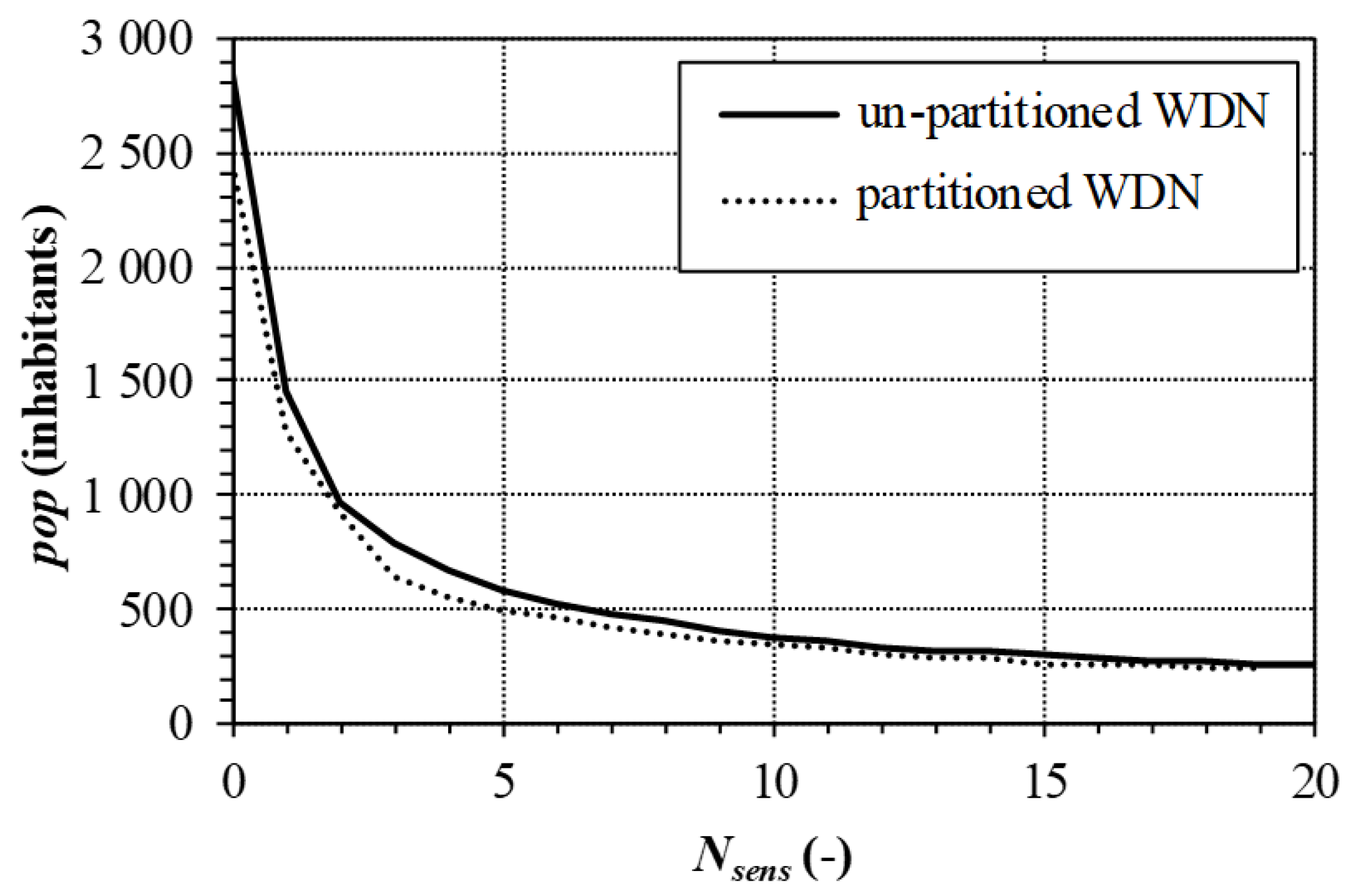
| 0 | 2806 | 0.0 | 2479 | 11.7 | 11.7 |
| 1 | 1438 | 48.8 | 1265 | 54.9 | 12.1 |
| 2 | 982 | 65.1 | 911 | 67.5 | 7.3 |
| 3 | 789 | 71.9 | 648 | 76.9 | 17.9 |
| 4 | 667 | 76.2 | 554 | 80.3 | 16.9 |
| 5 | 589 | 79.0 | 504 | 82.1 | 14.4 |
| 6 | 514 | 81.7 | 457 | 83.7 | 11.1 |
Publisher’s Note: MDPI stays neutral with regard to jurisdictional claims in published maps and institutional affiliations. |
© 2018 by the authors. Licensee MDPI, Basel, Switzerland. This article is an open access article distributed under the terms and conditions of the Creative Commons Attribution (CC BY) license (https://creativecommons.org/licenses/by/4.0/).
Share and Cite
Ciaponi, C.; Creaco, E.; Nardo, A.D.; Natale, M.D.; Giudicianni, C.; Musmarra, D.; Santonastaso, G.F. Optimal Sensor Placement in a Partitioned Water Distribution Network for the Water Protection from Contamination. Proceedings 2018, 2, 670. https://0-doi-org.brum.beds.ac.uk/10.3390/proceedings2110670
Ciaponi C, Creaco E, Nardo AD, Natale MD, Giudicianni C, Musmarra D, Santonastaso GF. Optimal Sensor Placement in a Partitioned Water Distribution Network for the Water Protection from Contamination. Proceedings. 2018; 2(11):670. https://0-doi-org.brum.beds.ac.uk/10.3390/proceedings2110670
Chicago/Turabian StyleCiaponi, Carlo, Enrico Creaco, Armando Di Nardo, Michele Di Natale, Carlo Giudicianni, Dino Musmarra, and Giovanni Francesco Santonastaso. 2018. "Optimal Sensor Placement in a Partitioned Water Distribution Network for the Water Protection from Contamination" Proceedings 2, no. 11: 670. https://0-doi-org.brum.beds.ac.uk/10.3390/proceedings2110670