Conditional or Pseudo Exact Tests with an Application in the Context of Modeling Response Times

Abstract

This paper treats a so called pseudo exact or conditional approach of testing assumptions of a psychometric model known as the Rasch model. Draxler and Zessin derived the power function of such tests. They provide an alternative to asymptotic or large sample theory, i.e., chi square tests, since they are also valid in small sample scenarios. This paper suggests an extension and applies it in a research context of investigating the effects of response times. In particular, the interest lies in the examination of the influence of response times on the unidimensionality assumption of the model. A real data example is provided which illustrates its application, including a power analysis of the test, and points to possible drawbacks.

1. Introduction

This contribution to the present special issue (Learning from Psychometric Data) particularly focuses on modeling techniques providing solutions to special data scenarios, i.e., the problem of high dimensional data with large numbers of items and/or small sample sizes as well as the consideration of reaction or response times. The availability of modern techniques like computerized psychological testing involves and supports, for instance, the consideration of response times in psychometric problems which, in turn, calls for respective statistical modeling and inferential approaches.

In particular, this paper deals with conditional or pseudo exact tests which have been developed in the context of testing assumptions of a psychometric model known as the Rasch model [1,2,3,4,5]. They may be called conditional since they are based on a conditional discrete probability distribution given the observed values of the sufficient statistics of both the person and item parameters of the Rasch model. They are pseudo exact since this conditional distribution is usually only approximated numerically by random sampling (apart from special cases which are mostly not of practical importance) using a Markov Chain Montel Carlo technique developed by Verhelst [4]. Draxler and Zessin [6] derived the power function of a broad class of conditional tests, in the one-sided case, and Draxler and Nolte [7] investigated their accuracy in terms of the numerical approximation of their power. Bayesian considerations have also been included by Draxler [8].

This work extends the discussion of Draxler and Zessin [6] by introducing two-sided tests and their power function with an application in the context of modeling the influence of reaction or response times on binary responses to so called mental paper folding tasks [9]. In particular, it deals with the question of multdimensionality of the person parameter, i.e., an ability to imagine paper folding. Thereby, the reaction time is treated as a metric covariate. Its effect is quantified by generalizing the Rasch model and introducing an additional parameter which yields a model with person, item, and conditional effect parameters given response times. The psychometric literature on modeling response times is rich and advanced quickly, in particular, in the last decade.

De Boeck and Jeon [10] give an overview of such approaches and categorize them into four classes. The approach discussed in this work can be assigned to their fourth category, i.e., response times as covariate models. On the one hand, these are models investigating a so-called speed-accuracy tradeoff (e.g., [11,12,13]) relating response times to accuracy (or power) and, on the other hand, generalized linear mixed models as discussed by, e.g., Goldhammer [14]. Van Breukelen [15] combines both of them with an application to data obtained from mental rotation tasks. A similar data example has been chosen for the present work. An interesting modeling approach suggested by Rijmen, De Boeck, and Leuven [16] may also be applied in a psychometric problem like the present. It generalizes the linear logistic test model [17] by introducing additional random effects for the items. Obviously, reaction times to the items can be considered as such random effects. Note that it is not the objective of the present paper to contribute a novel approach of modeling response times but rather to use the covariate model approach as a practically relevant example of an application of extended conditional or pseudo exact tests. An important practical advantage of these tests is that they are not based on asymptotic theory and thus, they are valid in small sample size scenarios too. They are a reasonable alternative to the usual chi square tests.

2. Motivation, Research Context, and Problem

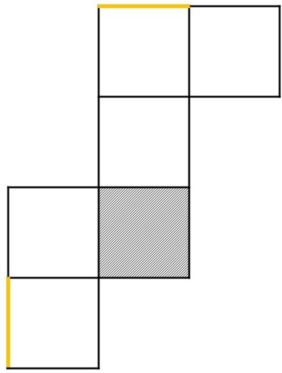
The main motivation for this paper stems from research on so called mental paper folding [9]. In mental paper folding, participants are shown a two-dimensional stimulus of a net of six connected squares as shown in Figure 1. Two lines on the outer parts of the net are highlighted in yellow. Participants are instructed to imagine folding the net into a cube as if they were folding a sheet of paper and indicate whether the two highlighted lines do overlap in the imagined cube or not.

In the present experiment data have been collected from 58 participants and a total of 428 stimuli or items. The latter can be distinguished according to the number of folds necessary to complete a task and the number of direction changes during folding. Slightly more than one third of all items do show overlapping highlighted yellow lines, the rest does not. The responses of the participants are binary, i.e., either correct or incorrect. Their response times were measured in milliseconds.

It is expected that response times are increasing with the number of folds and the number of direction changes during folding. Thus, one may raise the question of whether items with longer response times do measure a different ability than items with shorter response times. For instance, one may assume items with shorter response times measuring more a speed component and items with longer response times measuring more an ability to imagine paper folding. Furthermore, the present situation that the data are comprised of far more items than people is rather unusual in psychometric problems. Usually, it is the other way round. This calls for an approach and model, respectively, that in particular accounts for such a scenario.

3. Theoretical and Technical Treatment of the Problem

This Section presents one example of a conditional or pseudo exact test regarding the hypothesis of unidimensionality of the person parameter in the Rasch model quoted by Draxler and Zessin [6] and extends it in two respects, i.e., the treatment of a metric covariate instead of only categorical or binary ones and the discussion of a two-sided instead of a one-sided test.

3.1. A Conditional Probability Distribution Derived from a Generalized Rasch Model

Let $Y_{ij}\in \{0,1\}$ be the binary response of person $i=1,\cdots ,n$ to item $j=1,\cdots ,k$ and $X_j\in \mathbb{R}$ be a possibly random covariate. The latter may be, for instance, the (average) time measured for the n people to give a response to item j. Consider modeling the probability distributions of the Ys conditionally on the observed values of response times, i.e.,

$$P(Y_{ij}=y_{ij}\mid X_j=x_j)\propto exp\left(y_{ij}({\tau }_i+{\beta }_j+x_j{\delta }_i)\right),$$

(1)

where ${\tau }_i\in \mathbb{R}$ is a person parameter typically interpreted as an ability or attitude, ${\beta }_j\in \mathbb{R}$ is an item parameter quantifying the easiness or attractiveness of each item, and ${\delta }_i\in \mathbb{R}$ characterizes a conditional effect of each individual person given average response times per item. Hence, in this model each person is characterized by a multidimensional person parameter, i.e., it allows for items with shorter response times to measure different abilities than items with longer response times. Setting all $\delta$ parameters equal to 0 yields the Rasch model as a special case. The joint distribution of all binary responses of all n people to all k items is assumed to be given by

$$\prod _{i=1}^n\prod _{j=1}^{k}P(Y_{ij}=y_{ij}\mid X_j=x_j).$$

(2)

The factorizing criterion immediately shows that the statistics

$$\begin{array}{cc}\hfill & {\mathit{R}}^{\top }=(R_1,\cdots ,R_n),R_i=\sum _j{Y}_{ij},\hfill \\ \hfill & {\mathit{S}}^{\top }=(S_1,\cdots ,S_k),S_j=\sum _i{Y}_{ij},\hfill \\ \hfill & {\mathit{T}}^{\top }=(T_1,\cdots ,T_n),T_i=\sum _j{x}_j{Y}_{ij}\hfill \end{array}$$

are jointly sufficient for the family of distributions defined by (2), i.e., sufficient for all parameters of the model ${\mathit{\tau }}^{\top }=({\tau }_1,\cdots ,{\tau }_n)$, ${\mathit{\beta }}^{\top }=({\beta }_1,\cdots ,{\beta }_k)$, and ${\mathit{\delta }}^{\top }=({\delta }_1,\cdots ,{\delta }_n)$. Note that the former two sufficient statistics are the row and column sums of the response matrix, i.e., an $n\times k$ matrix containing the binary responses arranged in n rows and k columns.

Suppose the interest lies in making inferences about $\mathit{\delta }$, i.e., the conditional effects of response times, where $\mathit{\tau }$ and $\mathit{\beta }$ are treated as nuisance. To get rid of the influence of the nuisance parameters, consider the following conditional distribution given by

$$P(T_1=t_1,\cdots ,T_{n-1}=t_{n-1}\mid \mathit{R}=\mathit{r},\mathit{S}=\mathit{s})=\frac{{\sum }_{\mathrm{T}}exp\left({\mathit{t}}^{\top }\mathit{\delta }\right)}{{\sum }_{\Omega }exp\left({\mathit{t}}^{\top }\mathit{\delta }\right)}.$$

(3)

Note that one of the T statistics (one element of $\mathit{T}$) is not free given $\mathit{R}=\mathit{r}$ and $\mathit{S}=\mathit{s}$ and that the Ys need not be considered any more. It suffices to consider the conditional distribution of the Ts as a function of the Ys. They contain all the information needed for making inferences about $\delta$ because of their sufficiency property. For identifiability, let ${\delta }_k=0$. The denominator of the right side of (3) is a sum over the set $\Omega$ which denotes the set of all possible $n\times k$ matrices with row and column sums given by $\mathit{R}=\mathit{r}$ and $\mathit{S}=\mathit{s}$. The summation in the numerator has to be taken over a subset of $\Omega$, i.e., $\mathrm{T}\subseteq \Omega$, which is the set of $n\times k$ matrices satisfying $T_1=t_1,\cdots ,T_{n-1}=t_{n-1}$. Note that the hypergeometric distribution is a special case of the family of conditional distributions given by (3) [18]. In case of $\mathit{S}={\mathbf{1}}_k$ and assuming a binary covariate one yields the class of $(n-1)$-dimensional non-central hypergeometric distributions. If, additionally, $\mathit{\delta }={\mathbf{0}}_{n-1}$ one yields the central hypergeometric distribution. It is also easily verified from (3) that under the assumption $\mathit{\delta }={\mathbf{0}}_{n-1}$ every matrix contained in $\Omega$ has the same probability of being observed.

Treating (3) as a function of ${\mathit{\delta }}^{\top }=({\delta }_n,\cdots ,{\delta }_{n-1})$ and taking the logarithm one yields a conditional log likelihood function denoted by $\ell \left(\mathit{\delta }\right)$. The conditional maximum likelihood (CML) estimate of $\mathit{\delta }$ is defined by

$$\widehat{\mathit{\delta }}:=\underset{\mathit{\delta }\in {\mathbb{R}}^{n-1}}{\arg \max \ell \left(\mathit{\delta }\right)}.$$

General results of likelihood theory basically suggest that, under mild regularity conditions discussed by Andersen [19] and Pfanzagl [20],

$$\widehat{\mathit{\delta }}\stackrel{\mathbb{P}}{\to }\mathit{\delta }$$

and

$$\sqrt{k}\left(\widehat{\mathit{\delta }}-\mathit{\delta }\right)\stackrel{\mathbb{D}}{\to }{\mathcal{N}}_{n-1}\left({\mathbf{0}}_{n-1},\mathit{F}{\left(\mathit{\delta }\right)}^{-1}\right),k\to \infty ,$$

with $\mathit{F}(·)$ as the expected information matrix. Note that, in the present case, it is difficult to compute these CML estimates because of a complicated combinatorial problem involved in counting the total number of matrices in $\Omega$. A brief comment on this issue is provided in Section 3.3. For the purposes of this work, the estimates are expendable anyway.

Note that the modeling approach presented and the interpretation of the $\delta$ parameters can essentially be viewed as far more general. For example, the covariate may refer to person characteristics like gender as a binary covariate or age as a metric covariate. In such cases, the $\delta$ parameters do quantify linear effects of the person covariates on the log odds of the response probabilities to the items. Readers interested in various more examples, like testing the assumption of local independence, are referred to Draxler and Zessin [6] and Draxler [8]. The latter even treats a Bayesian extension.

3.2. A Two-Sided Conditional Test

Consider testing the hypothesis $\mathit{\delta }={\mathbf{0}}_{n-1}$ against the two-sided alternative $\mathit{\delta }\ne {\mathbf{0}}_{n-1}$. In principle, a number of statistical tests may be derived from the asymptotic or large sample properties of the CML estimator, i.e., the likelihood ratio [21,22], the Rao score [23], the Wald [24], and the gradient test [25,26,27], but these are not the focus of this paper. Note that, in the present problem, the term sample size has to be referred to the number of items since the parameter of interest $\mathit{\delta }$ refers to the people and thus, the variance of its estimate decreases with increasing number of items. A class of conditional or pseudo exact tests described by Draxler and Zessin [6] do not necessarily require large samples neither of people nor items. Consider the score function that takes a form which is well-known from the theory of the exponential family, i.e.,

$$\mathit{K}\left(\mathit{\delta }\right):=\frac{\partial \ell \left(\delta \right)}{\partial \delta }=\left(\begin{array}{c}{T}_1-E\left(T_1\right)\\ ⋮\\ T_{n-1}-E\left(T_{n-1}\right)\end{array}\right),$$

(4)

where $E\left(T_1\right),\cdots ,E\left(T_{n-1}\right)$ are the expected values of the $(n-1)$-dimensional distribution (3) and are obtained by

$$E\left(T_i\right)=\sum _{\min \left(T_i\right)}^{\max \left(T_i\right)}{t}_{i}P(T_i=t_i\mid \mathit{R}=\mathit{r},\mathit{S}=\mathit{s}),i=1,\cdots ,n-1,$$

(5)

and with

$$P(T_i=t_i\mid \mathit{R}=\mathit{r},\mathit{S}=\mathit{s})=\frac{{\sum }_{{\mathrm{T}}_i}exp\left({\sum }_{i=1}^n{t}_i{\delta }_i\right)}{{\sum }_{\Omega }exp\left({\sum }_{i=1}^n{t}_i{\delta }_i\right)}.$$

(6)

The subset ${\mathrm{T}}_i\subseteq \Omega$ is comprised of those $n\times k$ matrices satisfying $T_i=t_i$. The range of values one can possibly observe for $T_i$, i.e., from $\min \left(T_i\right)$ to $\max \left(T_i\right)$, depends on the observed values of $\mathit{R}$ and $\mathit{S}$ and response times. Consider

$$U={\mathit{K}}^{\top }(\mathit{\delta }={\mathbf{0}}_{n-1})\mathit{K}(\mathit{\delta }={\mathbf{0}}_{n-1})$$

(7)

as the test statistic, i.e., sum of squared elements of the score function evaluated at $\mathit{\delta }={\mathbf{0}}_{n-1}$ (under the hypothesis to be tested). Other reasonable choices of the test statistic may be the sum of the absolute values of the elements of the score function or the score function itself (in the one-sided case). An exact p value is obtained by computing the test statistic for every matrix in $\Omega$ and counting the number of matrices yielding a value for the test statistic being not smaller than the value obtained for the observed matrix. Thus, CML estimates of $\delta$ need not be computed at all to obtain the exact distribution of the test statistic under the hypothesis to be tested. One only has to count the number of matrices in the set $\Omega$ but this is nontrivial. Some comments on this are given in Section 3.3.

This $(n-1)$-dimensional testing procedure may be reduced in dimensionality where needed in a particular case, e.g., when considering only single people. One simply selects the desired subset of elements (people) of the vector-valued score function (4) and proceeds as described to compute the test statistic U and the respective p value of the test.

The power function of the test is a function of $\mathit{\delta }$ given a critical region. Let $\mathrm{C}\subseteq \Omega$ denote the critical region of the test and $\alpha$ its size, i.e., the probability of the error of the first kind. Let C be composed of those $n\times k$ matrices in $\Omega$ that yield the $100\alpha$ percent largest values of the test statistic U. Then, the power function is obtained by

$$\beta \left(\mathit{\delta }\right)=\sum _{\mathrm{C}}P(T_1=t_1,\cdots ,T_{n-1}=t_{n-1}\mid \mathit{R}=\mathit{r},\mathit{S}=\mathit{s}).$$

(8)

Note that, because of the underlying discrete distribution (3), conservatism issues and suggestions of resolving them well-known from discussions on Fisher’s exact test (e.g., [28]) play a role in this case too, specifically, in scenarios of very small person and item numbers and extreme true values of the parameters. It should also be remarked that in the present case of a multidimensional and two-sided testing problem, the described choice of the critical region C cannot be considered optimal from a theoretical perspective. It can indeed be viewed as reasonable and may serve the present practical purpose well enough, but it is generally not unbiased and not uniformly most powerful.

3.3. Computational Issues

Counting the exact total number of matrices in $\Omega$ is not an easy task in realistic cases with the usual numbers of people and items typically occurring in psychometric research. Only recently, Miller and Harrison [29] suggested a recursive counting algorithm and solved this complicated combinatorial problem of discrete mathematics. Nonetheless, the computational effort in case of $n+k>100$ is still too demanding for the usual RAM capacities of today’s desktop machines. Thus, for practical and computational purposes, numerical and random sampling techniques may be used, i.e., sequential importance sampling [30,31] and a Markov Chain Monte Carlo (MCMC) approach suggested by Verhelst verhelst2008.

The MCMC approach is probably the most promising in terms of practicality and computing times. It is readily accessible as an R package [5]. It is capable of handling larger numbers of matrices (larger numbers of people and items) and is computationally very efficient compared to other approaches [7]. Briefly speaking, in this approach, the stationary distribution of the Markov chain is given by the discrete uniform distribution over all elements in $\Omega$. Hence, it provides random draws with approximate equal probabilities for each element (matrix) contained in $\Omega$. Having drawn a random sample of $n\times k$ matrices from $\Omega$ the conditional distribution (3) and that of the test statistic U as well as the p value can be arbitrarily well approximated. That is why such a test may be called conditional and/or pseudo exact.

4. Data Analysis and Results

The example data contain the binary responses of 58 people to 428 items as well as the response times per person and item. A few more people were originally available but these had to be excluded since their response times appeared to be unrealistic and they did not behave according to instructions. Response times have been averaged over all people for each item. Thus, each of the 428 items is characterized by a mean response time which is considered as a metric covariate in the model.

For the numerical approximation of the conditional distribution (3), the conditional distribution of the test statistic U, and the p value of the conditional test, respectively, Verhelst’s MCMC approach and the respective R package RaschSampler [5] has been used. The package is restricted to matrices with maximum numbers of rows and columns, i.e., people and items, of $2^{12}=4096$ and $2^7=128$. To meet these requirements in the present example the observed matrix of binary responses has been transposed yielding a matrix with 428 rows (items) and 58 columns (people). The number of matrices drawn for the computations has been set to 8000 (the package limits the maximum number to $2^{13}=8192$). Some important control parameters of the Markov Chain like burn in phase and step parameter have been chosen in a reasonable manner to ensure reliable results and independence of the draws, i.e., only every 50th matrix drawn was accepted for the sample used for the computations. According to results of Draxler and Nolte [7] this seems to be a sufficient number. The procedure of drawing a random sample of 8000 matrices has been replicated a number times to check the accuracy of the computations. A commented R code for such an analysis is provided in the Appendix A.

The results are as follows. The approximated p value of the overall test that all $58-1=57$ free $\delta$ parameters are 0 against the two-sided alternative that at least one of them is not 0 resulted to be 0. Thus, not a single one of all matrices drawn yielded a value of the test statistic U that is greater or equal to the value obtained for the observed matrix, i.e., $U=108.416$ for the observed matrix whereas the maximum value of the 8000 matrices drawn resulted to be $57.52$ (minimum value $8.958$, first quartile $22.37$, median $25.79$, mean $26.26$, third quartile $29.72$). Thus, they are distinctly lower than the observed value. This result is unambiguous. It is very likely that the exact p value is very close to 0. The result does not support the unidimensionality assumption of the Rasch model.

A separate analysis of the responses of each single person yields the following results as shown in

Table 1. Results of analysis of the responses of individual people.

Pers. No.	p Value	Score	No. Corr.	Pers. No.	p Value	Score	No. Corr.
1	0.236	0.543	420	30	0.154	−1.127	391
2	0.687	0.296	398	31	<0.001	6.889	251
3	0.717	0.224	411	32	0.023	1.045	419
4	0.003	3.190	259	33	0.090	−0.679	422
5	0.278	−0.876	387	34	0.645	0.399	370
6	0.795	−0.162	411	35	0.001	−2.155	403
7	0.024	1.882	383	36	0.686	−0.111	426
8	0.758	0.176	416	37	0.578	0.360	408
9	0.246	0.342	425	38	0.116	−1.278	385
10	0.915	−0.085	398	39	0.001	−3.142	338
11	0.067	1.944	260	40	0.111	−0.637	422
12	0.262	0.688	412	41	0.739	0.233	404
13	0.762	0.157	418	42	0.152	0.877	411
14	0.607	0.386	400	43	0.910	0.091	402
15	0.194	−0.777	412	44	0.356	−0.737	394
16	0.937	−0.031	417	45	0.634	0.269	413
17	0.439	−0.669	385	46	0.891	0.068	413
18	0.471	−0.290	423	47	0.848	0.071	423
19	0.003	−1.550	416	48	-	-	-
20	0.003	1.919	408	49	0.251	0.655	414
21	0.944	0.054	391	50	0.295	−0.774	397
22	0.893	0.082	399	51	0.265	0.797	400
23	0.632	0.409	376	52	0.224	−0.982	390
24	0.924	−0.076	403	53	0.002	−2.043	408
25	0.006	−1.256	419	54	0.209	0.632	418
26	0.114	−1.257	392	55	0.050	−0.964	418
27	0.471	−0.320	421	56	0.494	−0.323	419
28	0.218	−0.701	414	57	0.153	−0.524	423
29	0.295	−0.694	406	58	0.574	−0.458	386

Note. Person 48 excluded. The values of the test statistic U are obtained by squaring the observed scores.

. Note that person 48 is excluded from the analysis since the responses of this person are completely uninformative, i.e., person 48 responded correctly to all 428 items. The lowest p values, i.e., <0.01, are obtained for people 31, 35, 39, 53, 19, 4, 20, and 25. Thus, the responses of these eight people may be considered hardly compatible with the assumption of a unidimensional person parameter. If these people were excluded from the analysis, i.e., one tested the hypothesis that the $\delta$ parameters of the rest of people equals 0, one would yield a p value of $0.13$ for the overall test. Thus, the undimensionality assumption seems to be all right for the rest of the respondents.

Table 1 also shows the observed values of the score function, i.e., the respective elements of the vector given by (4). The score provides a more detailed interpretation of the meaning of deviation from unidimensionality. Persons with a positive sign of their score do perform better than people with a negative sign on items with longer response times, whereas it is the other way round regarding items with shorter response times. For example, person 39 performs better than person 31 on items with shorter response times but person 39 performs worse than person 31 on items with longer response times. The observed score for person 39 is $-3.142$ and for person 31 it is 6.889. Thus, the longer response times the worse is the performance of person 39 compared to person 31. The shorter response times the better is person 39 compared to person 31.

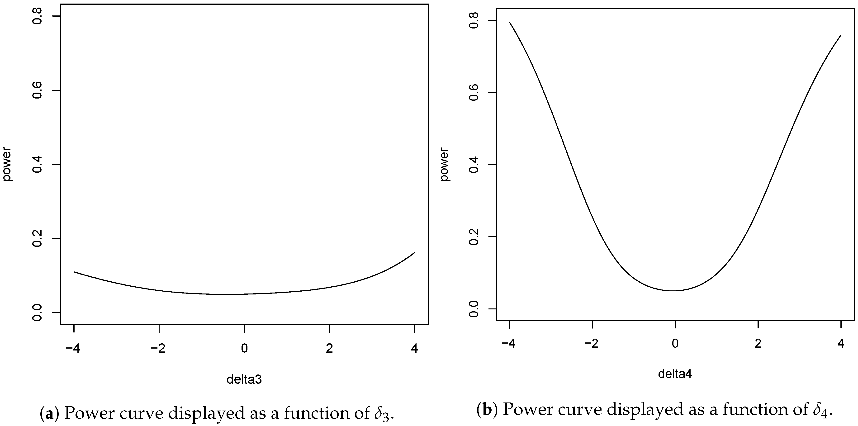
An additional brief power analysis of the test yields the following results. As an example consider the comparison of people 3 and 4. Note that the responses of person 4 are much more informative in respect of ${\delta }_4$ than the responses of person 3 concerning ${\delta }_3$ are. As can be seen in Table 1, this is because the number of correct responses of person 3 is distinctly higher and much closer to the maximum value of 428 than it is in respect of person 4. This has an effect on the power function of the test. Figure 2 shows on the left panel the power of the overall test as a function of ${\delta }_3$ (person 3) while all other $\delta$ parameters are set to 0. On the right panel, one can see the power function referring to person 4, i.e., as a function of ${\delta }_4$ given all other $\delta$ parameters being set to 0. The size of the critical region $\alpha$ has been set to $0.05$. The difference between the two curves is striking. Regarding person 4, the power increases much steeper than concerning person 3. This should be taken into account for the practical interpretation of the results. The p values in Table 1 do not necessarily show a problem of the unidimensionality assumption in respect of person 3 but taking into account the power analysis such an interpretation should be taken with caution. The deviation of ${\delta }_3$ from 0, i.e., person 3’s true amount of deviation from unidimensionality, must obviously be distinctly larger to achieve an acceptable power than in respect of person 4. A similar interpretation may be in order in respect of several other people whose total number of correct responses are close to the maximum.

Note that Figure 2 shows the power function of the overall test which has 57 degrees of freedom or free $\delta$ parameters. Thus, assuming only one of the parameters to deviate from 0 while assuming all others to be 0 will in general not yield high power values. For instance, as can be seen in Figure 2, the power is approximately only $0.1$ if ${\delta }_4=1$ given all other $\delta$ parameters being set to 0, and it is even lower if ${\delta }_3=1$ given, again, all other $\delta$ parameters being 0. Surely, if one assumes more than one $\delta$ parameter deviating simultaneously from 0 the power will generally be larger.

5. Final Remarks

From the psychometric point of view, it is remarkable that the number of items does far exceed the number of people in the present data example. A consequence is that person abilities, i.e., $\tau$ parameters of the model, and the individual conditional effects of response times per person, i.e., $\delta$ parameters, can be measured (or estimated) very accurately compared to the item difficulties. Statistically speaking, the information in the data about the $\tau$ and $\delta$ parameters is high compared to that of the $\beta$ parameters. Since the $\delta$ parameters are those of interest the approach presented, i.e., the model given by (1) and the conditional distribution (3) on which the test is based, is quite a reasonable and suitable choice for making inferences about the $\delta$ parameters.

In commenting on the data analysis, it should be remarked that the statistical information contained in the present data is at least partly low. The items seem to be too easy for many people. Consequently, the power of the test with respect to single $\delta$ parameters yields partly very low values, i.e., the power considered as a function of one single $\delta$ parameter (a single person) at a time while setting all other $\delta$ parameters to 0. Thus, for some people the deviation from the undimensionality assumption of the Rasch model must obviously be extremely large in order to achieve a desirable power. Nonetheless, the results of the analysis reveal or, to be careful, at least hint at violations of undimensionality for several people. The true effects of this violation seem to be pretty large for some people, i.e., their true $\delta$ parameters seem to be far from 0.

The practical interpretation of the observed violations of or deviations from the unidimensionality assumption of the Rasch model is not easy. A possible and simple interpretation may be that, for several respondents, items with shorter response times are tending to measure more a speed component whereas items with longer response times are measuring more a power component of an ability to imagine paper folding.

Another possible interpretation in case of a rejection of the hypothesis that the $\delta$ parameters are 0 may be that the items do discriminate differently and the discriminations are correlated positively with the mean reaction times. Such a scenario does not necessarily indicate a multidimensional model. It may also be modeled by considering a discrimination parameter for the items in a still unidimensional model like the well-known 2 PL model.

References

- Rasch, G. Probabilistic Models for Some Intelligence and Attainment Tests; Danish Institute for Educational Research: Copenhagen, Denmark, 1960. [Google Scholar]
- Fischer, G.H.; Molenaar, I.W. Rasch Models. Foundations, Recent Developments and Applications; Springer: New York, NY, USA, 1995. [Google Scholar]
- Ponocny, I. Nonparametric Goodness-of-Fit Tests for the Rasch Model. Psychometrika 2001, 66, 437–459. [Google Scholar] [CrossRef]
- Verhelst, N.D. An Efficient Mcmc Algorithm to Sample Binary Matrices with Fixed Marginals. Psychometrika 2008, 73, 705–728. [Google Scholar] [CrossRef]
- Verhelst, N.D.; Hatzinger, R.; Mair, P. The Rasch Sampler. J. Stat. Softw. 2007, 20, 1–14. [Google Scholar] [CrossRef]
- Draxler, C.; Zessin, J. The Power Function of Conditional Tests of the Rasch Model. ASTA Adv. Stat. Anal. 2015, 99, 367–378. [Google Scholar] [CrossRef]
- Draxler, C.; Nolte, J.P. Computational Precision of the Power Function for Conditional Tests of Assumptions of the Rasch Model. Open J. Stat. 2018, 8, 873–884. [Google Scholar] [CrossRef] [Green Version]
- Draxler, C. Bayesian Conditional Inference for Rasch Models. ASTA Adv. Stat. Anal. 2018, 102, 245–262. [Google Scholar] [CrossRef]
- Shepard, R.N.; Feng, C. A chronometric study of mental paper folding. Cogn. Psychol. 1972, 3, 228–243. [Google Scholar] [CrossRef]
- De Boeck, P.; Jeon, M. An overview of models for response times and processes in cognitive tests. Front. Psychol. 2019, 10, 102. [Google Scholar] [CrossRef] [Green Version]
- Roskam, E.E. Towards a psychometric theory of intelligence. In Progress in Mathematical Psychology, 1st ed.; Roskam, E.E., Suck, R., Eds.; Elsevier Science: Amsterdam, The Netherlands, 1987; Volume 1, pp. 151–174. [Google Scholar]
- Verhelst, N.D.; Verstralen, H.H.F.M.; Jansen, M.G. A logistic model for time-limit tests. In Handbook of Modern Item Response Theory, 1st ed.; van der Linden, W.J., Hambleton, R.K., Eds.; Springer: West New York, NJ, USA, 1997; Volume 1, pp. 169–185. [Google Scholar]
- Wang, T.; Hanson, B.A. Development and calibration of an item response model that incorporates response time. Appl. Psychol. Meas. 2005, 29, 323–339. [Google Scholar] [CrossRef] [Green Version]
- Goldhammer, F.; Steinwascher, M.A.; Kroehne, U.; Naumann, J. Modeling individual response time effects between and within experimental speed conditions: A GLMM approach for speeded tests. Br. J. Math. Stat. Psychol. 2017, 70, 238–256. [Google Scholar] [CrossRef]
- van Breukelen, G.J.P. Psychometric modeling of response speed and accuracy with mixed and conditional regression. Psychometrika 2005, 70, 359–376. [Google Scholar] [CrossRef]
- Rijmen, F.; De Boeck, P.; Leuven, K.U. The random weights linear logistic test model. Appl. Psychol. Meas. 2002, 26, 271–285. [Google Scholar] [CrossRef]
- Fischer, G.H. Linear logistic test model as aninstrument in educational research. Acta Psychol. 1973, 37, 359–374. [Google Scholar] [CrossRef]
- Draxler, C. A Note on a Discrete Probability Distribution Derived from the Rasch Model. Adv. Appl. Stat. Sci. 2011, 6, 665–673. [Google Scholar]
- Andersen, E.B. Asymptotic properties of conditional maximum-likelihood estimators. J. R. Stat. Soc. Ser. B Methodol. 1970, 32, 283–301. [Google Scholar] [CrossRef]
- Pfanzagl, J. On the consistency of conditional maximum likelihood estimators. Ann. Inst. Stat. Math. 1993, 45, 703–719. [Google Scholar] [CrossRef]
- Neyman, J.; Pearson, E.S. On the use and interpretation of certain test criteria for purposes of statistical inference. Biometrika 1928, 20 A, 263–294. [Google Scholar]
- Wilks, S.S. The large sample distribution of the likelihood ratio for testing composite hypotheses. Ann. Math. Stat. 1938, 9, 60–62. [Google Scholar] [CrossRef]
- Rao, C.R. Large sample tests of statistical hypotheses concerning several parameters with applications to problems of estimation. Proc. Camb. Philos. Soc. 1948, 44, 50–57. [Google Scholar]
- Wald, A. Test of statistical hypotheses concerning several parameters when the number of observations is large. Trans. Am. Math. Soc. 1943, 54, 426–482. [Google Scholar] [CrossRef]
- Terrell, G.R. The gradient statistic. Comput. Sci. Stat. 2002, 34, 206–215. [Google Scholar]
- Lemonte, A.J. The Gradient Test. Another Likelihood-Based Test; Academic Press: London, UK, 2016. [Google Scholar]
- Draxler, C.; Kurz, A.; Lemonte, A.J. The gradient test and its finite sample size properties in a conditional maximum likelihood and psychometric modeling context. Commun. Stat. Simul. Comput. 2020, 1–19. [Google Scholar] [CrossRef]
- Agresti, A. Categorical Data Analysis, 3rd ed.; John Wiley & Sons: Hoboken, NJ, USA, 2013. [Google Scholar]
- Miller, J.W.; Harrison, M.T. Exact Sampling and Counting for Fixed-Margin Matrices. Ann. Stat. 2013, 41, 1569–1592. [Google Scholar] [CrossRef] [Green Version]
- Chen, Y.; Diaconis, P.; Holmes, S.P.; Liu, J.S. Sequential Monte Carlo Methods for Statistical Analysis of Tables. J. Am. Stat. Assoc. 2005, 100, 109–120. [Google Scholar] [CrossRef]
- Chen, Y.; Small, D. Exact Tests for the Rasch Model via Sequential Importance Sampling. Psychometrika 2005, 70, 11–30. [Google Scholar] [CrossRef]
Figure 1.
Example of a mental paper folding task.
Figure 2.
Power function of the overall test.