
Variational Amplitude Amplification for Solving QUBO Problems

Air Force Research Laboratory Information Directorate, Rome, NY 13441, USA
*
Author to whom correspondence should be addressed.
Quantum Rep. 2023, 5(4), 625-658; https://0-doi-org.brum.beds.ac.uk/10.3390/quantum5040041
Submission received: 31 July 2023
/
Revised: 28 August 2023
/
Accepted: 22 September 2023
/
Published: 1 October 2023
(This article belongs to the Special Issue Quantum Computing: A Taxonomy, Systematic Review, and Future Directions)
Abstract
:We investigate the use of amplitude amplification on the gate-based model of quantum computing as a means for solving combinatorial optimization problems. This study focuses primarily on quadratic unconstrained binary optimization (QUBO) problems, which are well-suited for qubit superposition states. Specifically, we demonstrate circuit designs which encode QUBOs as ‘cost oracle’ operations , which distribute phases across the basis states proportional to a cost function. We then show that when is combined with the standard Grover diffusion operator , one can achieve high probabilities of measurement for states corresponding to optimal and near optimal solutions while still only requiring O() iterations. In order to achieve these probabilities, a single scalar parameter is required, which we show can be found through a variational quantum–classical hybrid approach and can be used for heuristic solutions.
1. Introduction
Amplitude amplification is a quantum algorithm strategy that is capable of circumventing one of quantum computing’s most difficult challenges: probabilistic measurements. Originally proposed by Grover in 1996 [1], and later shown to be optimal [2,3], the combination of his oracle and ‘diffusion’ operators is able to drive a quantum system to a superposition state where one (or multiple) basis state(s) has nearly 100% probability of being measured. Since then, many researchers have contributed to the study of and [4,5,6,7,8,9], seeking to better understand how the fundamental nature of amplitude amplification is dependent on these two operators. Similarly, the aim of this study is to further extend the capabilities of amplitude amplification as a means for solving combinatorial optimization problems using gate-based quantum computers. In particular, we focus on amplitude amplification’s ability to solve QUBO (quadratic unconstrained binary optimization) problems. The best quantum algorithm for solving this problem is an open question, with notable research efforts in variational approaches [10,11,12] and quantum annealing [13,14,15,16], as well as within amplitude amplification [17,18].
This study is a continuation of our previous work [19], in which we demonstrated an oracle design which was capable of encoding and solving a weighted directed graph problem. The motivation for this oracle was to address a common criticism of [18,20,21,22,23], namely, that the circuit construction of oracles too often hardcodes the solution it aims to find, negating the use of quantum entirely. Similar to other recent studies [24,25,26,27], we showed that this problem can be solved at the circuit depth level by avoiding gates such as control-Z for constructing the oracle and instead using phase and control-phase gates (P() and CP()). However, simply changing the phase produced from to something other than is not enough [28,29,30,31,32,33]. Our oracle construction applies phases to not only a desired marked state(s), but states in the full Hilbert Space. The phase each basis state receives is proportional to the solutions of a weighted combinatorial optimization problem, for which the diffusion operator can be used to boost the probability of measuring states that correspond to optimal solutions.
The consequence of using an oracle operation that applies phases to every basis state is an interesting double-edged sword. As we show in Section 2, Section 3 and Section 4, and later in Section 7, the use of phase gates allows for amplitude amplification to encode a broad scope of combinatorial optimization problems into oracles, which we call ‘cost oracles’ . In particular, we demonstrate the robustness of amplitude amplification for solving these kinds of optimization problems with asymmetry and randomness [34,35,36]. However, the tradeoff for solving more complex problems is twofold. First, in contrast to Grover’s oracle, when using it is only able to achieve peak measurement probabilities up to 70–90% for problems composed of 20–30 qubits. In Section 6 we show that these probabilities are high enough for quantum to reliably find optimal solutions, which notably are achieved using the same O( ) iterations as standard Grover’s [1,2,3] (wher N is the total number of superposition states and M is the number of marked states).
The second and more challenging tradeoff when using is that the success of amplitude amplification is largely dependant on the correct choice of a single free parameter [19]. This scalar parameter is multiplied into every phase gate for the construction of (P() and CP()), and is responsible for transforming the numeric scale of a given optimization problem to values which form a range of approximately . This in turn is what allows for reflections about the average amplitude via to iteratively drive the probability of desired solution states up to 70–90%. The significance of , and the challenges in determining it experimentally, are a major motivation for this study. In particular, the results in Section 5 demonstrate that there is a range of values for which many optimal solutions can be made to become highly probable. Importantly, this allows our approach to be used as a heuristic quantum algorithm, similar to other leading strategies [10,11,12,17]. Even better, in Section 5 we show that there is an observed correlation between the ranked order of solutions and the values at which they achieve peak probabilities. This underlying correlation is a core finding of this study, and in Section 6 we discuss how it can be used to construct a hybrid classical–quantum algorithm. This promising result indicates that our amplitude amplification strategy can be synergized with classical computing techniques, in particular greedy algorithms [37,38].
Layout
The layout of this study is as follows. Section 2 begins with the mathematical formalism for the optimization problem we seek to solve using amplitude amplification. Section 3 and Section 4 discuss the construction of the problem as a quantum circuit, the varying degrees of success to be expected from optimization problems generated using random numbers, and the conditions for which these successes can be experimentally realized. In Section 5, we explore the role of from a heuristic perspective, whereby we demonstrate that many near optimal solutions are capable of reaching significant probabilities of measurement. Section 6 is a primarily speculative discussion, theorizing about how the collective results presented in Section 5 could coalesce into a hybrid quantum–classical variational algorithm. Finally, Section 7 completes the study with additional optimization problems that can be constructed as oracles and solved using amplitude amplification.
2. QUBO Definitions
We begin by outlining the optimization problem which serves as the focus for this study: QUBO (quadratic unconstrained binary optimization). The QUBO problem has many connections to important fields of computer science [39,40,41,42,43], making it relevant for demonstrating quantum’s potential for obtaining solutions. To date, the two most successful quantum approaches to solving QUBOs are annealing [13,14,15,16] and QAOA [10,11,44,45], with a great deal of interest in comparing the two [46,47,48]. Shown below in Equation (1) is the QUBO cost function, C(X), which we seek to solve using our quantum algorithm.
The function C(X) evaluates a given binary string X of length N composed of individual binary variables . Together, the total number of unique solutions to each QUBO is , which is the number of quantum states producible from N qubits. Throughout this study, we use the subscripts X and C(X) when referring to individual solutions and C(X) when discussing a cost function more generally.
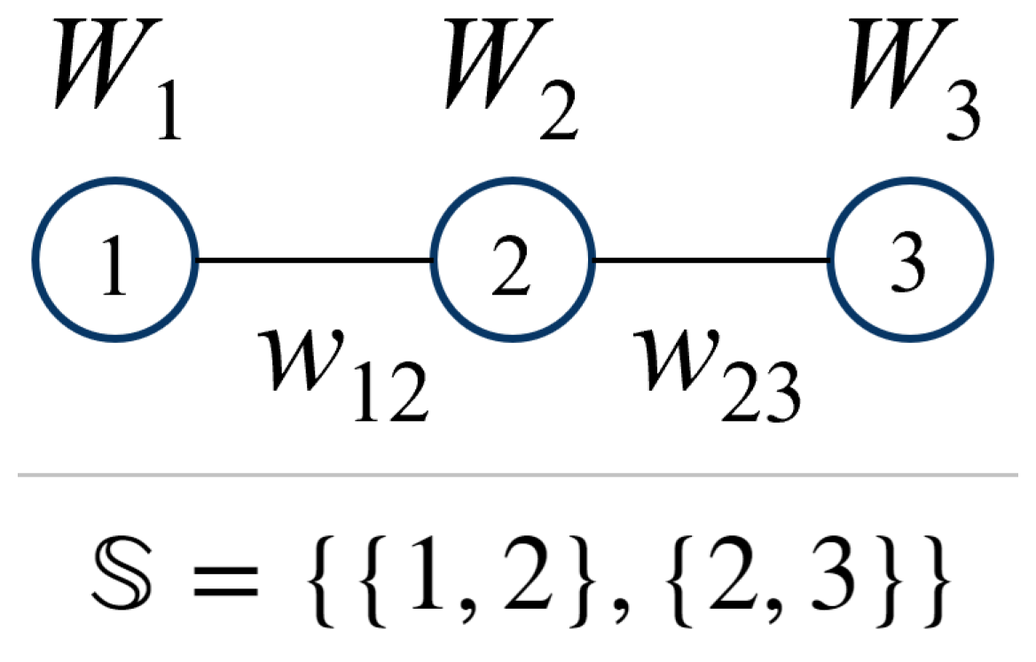
As shown in Equation (1), a QUBO is defined by two separate summations of weighted values. The first summation evaluates weights associated with each individual binary variable, while the second summation accounts for pairs of variables which share a weighted connection . In this study, we adopt the typical interpretation of QUBOs as graph problems, whereby each binary variable represents a node. We can then define the connectivity of a QUBO graph using the set , which itself is a collection of sets that describe each pair of nodes and that share a connection. See Figure 1 below for an example.
The interest of this study is to use a quantum algorithm to find either X or X, which are the solutions which minimize/maximize the cost function C(X), respectively. For all QUBOs analyzed in the coming sections, the weight values and are restricted to integers randomly selected from a uniform distribution, as shown below in Equations (2) and (3).
In Section 5, we discuss the consequences of choosing weight values in this manner and its advantage for quantum. However, nearly all of the results shown throughout this study are applicable to the continuous cases for and as well, with the one exception being the results in Section 5.4.
Linear QUBO
The cost function provided in Equation (1) is applicable to any graph structure as long as every node and edge is assigned a weight. For this study, we focus on one specific , which we refer to as a ‘linear QUBO’. The connectivity of these graphs is as follows:
As the name suggests, linear QUBOs are graphs for which every node has connectivity with exactly two neighboring nodes excepting the first and final nodes. The motivation for studying QUBOs of this nature is their efficient realizability as quantum circuits, which is discussed in the next section.
3. Amplitude Amplification
The quantum strategy for finding the optimal solutions to C(X) investigated in this study is amplitude amplification [4,5,6,7,8,9], which is the generalization of Grover’s algorithm [1]. The full algorithm is shown below in Algorithm 1, which is almost identical to Grover’s algorithm except for the replacement of Grover’s oracle with our cost oracle .
| Algorithm 1 Amplitude Amplification Algorithm |
|
By interchanging different oracle operations into Algorithm 1, various problem types can be solved using ampltitude amplification. For example, Grover’s original oracle solves an unstructured search, whereas here we are interested in optimal solutions to a cost function. Later, in Section 7, we discuss further oracle adaptations and the problems that they solve. For all oracles, we use the standard diffusion operator provided below in Equation (5).
This operation achieves a reflection about the average amplitude whereby every basis state in is reflected around their collective mean in the complex plane. This operation causes states’ distance from the origin to increase or decrease based on their location relative to the mean, which in turn determines their probability of measurement. Therefore, a successful amplitude amplification is able to drive the desired basis state(s) as far from the origin as possible up to a maximum distance of 1 (a measurement probability of 100%).
3.1. Solution Space Distribution
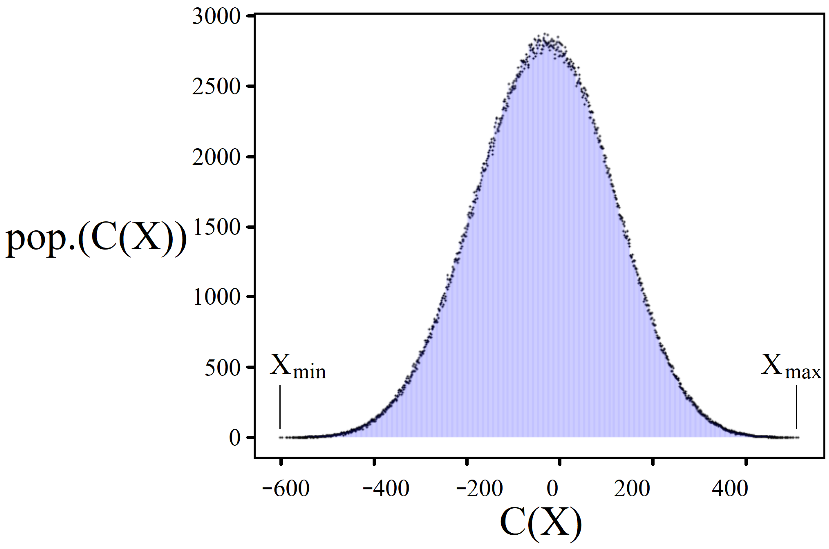
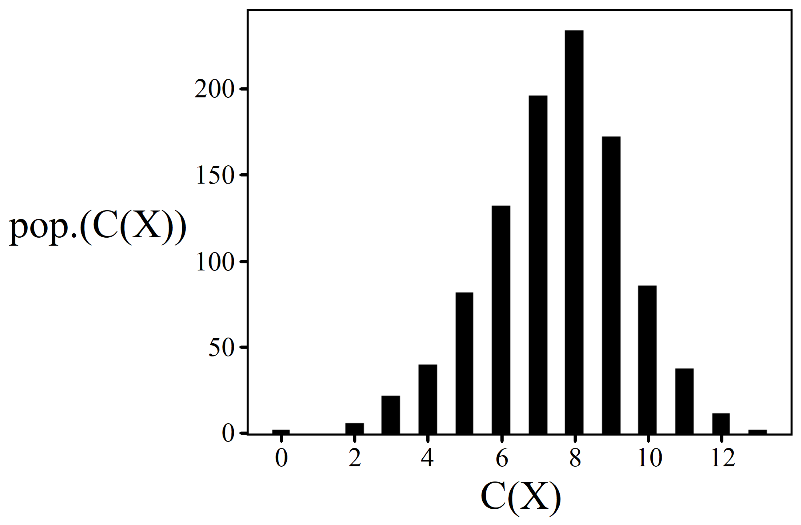
A prerequisite for the success of amplitude amplification as demonstrated in this study is an optimization problem’s underlying solution space distribution, that is, the manner in which all possible solutions to the problem are distributed with respect to one another; for QUBOs, these are the possible C(X) cost function values. Shown below in Figure 2 is a histogram of one such solution space distribution for the case of a linear QUBO with length 20 according to Equations (1)–(4). The x-axis represents all possible cost function evaluations and the y-axis is the corresponding number of unique X solutions that result in the same C(X) value.
Depicted in Figure 2 are all possible solutions to an example linear QUBO. Because this QUBO was generated from randomized weights, the combination of the Law of Large Numbers [49] and Central Limit Theorem [50] predicts that its underlying solution space should be approximately Gaussian [51] in shape, as provided by Equation (6).
Indeed, the histogram is approximately Gaussian; importantly, however, it has imperfections resulting from the randomized weights. At large enough problem sizes (around ), these imperfections have minimal impact on a problem’s aptitude for amplitude amplification, which is one result from our previous study [19]. Similarly, another recent study [26] has demonstrated that, in addition to symmetric Gaussians, solution space distributions for both skewed Gaussians and exponential profiles lead to successful amplitude amplifications. The commonality between these three distribution shapes is that they all possess large clusters of solutions that are sufficiently distanced from the optimal solutions that we seek to boost. This can be seen in Figure 2 as the location of X and X as compared to the central peak of the Gaussian. When appropriately encoded as an oracle , these clusters serve to create a mean point in the complex plane which the optimal solution(s) use to reflect about and increase in probability.
3.2. Cost Oracle
In order to use Algorithm 1 to find the optimal solution to a given cost function, we must construct a cost oracle which encodes the weighted information and connectivity of the problem. In our previous study, we referred to this operation as a ‘phase oracle’ [19], and it has similarly been called a ‘subdivided phase oracle’ SPO [25,26] or ‘non-Boolean oracle’ [27]. Although how one constructs is problem-specific, the general strategy is to primarily use two quantum gates, as shown below in Equations (7) and (8).
The single and two-qubit gates P() and CP() are referred to as phase gates, sometimes known as R() and CR() due to their effect of rotating a qubit’s state around the z-axis of the Bloch sphere. Mathematically, they are capable of applying complex phases, as shown below.
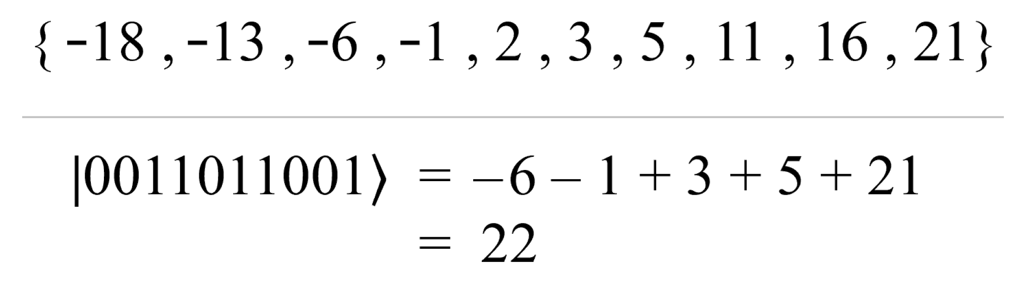
Applying P() to a qubit only affects the state, leaving unchanged, and similarly only for CP(). However, this is exactly what we need in order to construct C(X) from Equation (1). When evaluating a particular binary string X classically, only instances where the binary values are equal to 1 yield non-zero terms in the summations. For quantum, each binary string X is represented by one of the basis states . Thus, our quantum cost oracle can replicate C(X) by using P() and CP() to only effect basis states with qubits in the and states.
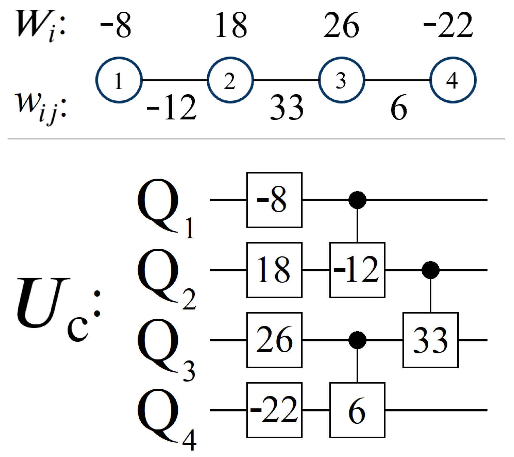
Shown above in Figure 3 is an example of a 4-qubit QUBO cost oracle, where the weighted values and are used as the parameters for the various phase gates. This quantum circuit can be generalized to encode any QUBO as defined in Equation (1): single qubit P() gates for the summation of terms and two-qubit CP() gates for the summation of terms. If we wish to go beyond quadratic cost function terms in C(X), then we can use N-qubit control phase gates to encode weights which depend on N binary variables.
Although incomplete (see the next section), we can use this oracle circuit to demonstrate quantum’s ability to encode a cost function C(X). For example, consider the binary solution X and the corresponding quantum basis state . The classical evaluation of this solution is as follows:
Now, let us compare this to the phase of after applying :
The phase acquired in Equation (12) is equivalent to the classical evaluation shown in (11), which means that is an accurate encoding of C(X). If we were to now apply to the equal superposition state (Step 2 in Algorithm 1), all basis states would receive phases equal to their cost function value. This is the advantage that quantum has to offer: simultaneously evaluating all possible solutions of a cost function through superposition.
3.3. Scaling Parameter
While the cost oracle shown in Figure 3 is capable of reproducing C(X), its use in Algorithm 1 does not yield the optimal solution X or X. This is because quantum phases are modulo, which is problematic if the numerical scale of C(X) exceeds a range of . Consequently, if two quantum states receive phases that differ by a multiple of , then they both undergo the amplitude amplification process identically. If this happens unintentionally via , then our cost oracle cannot be used to minimize or maximize C(X).
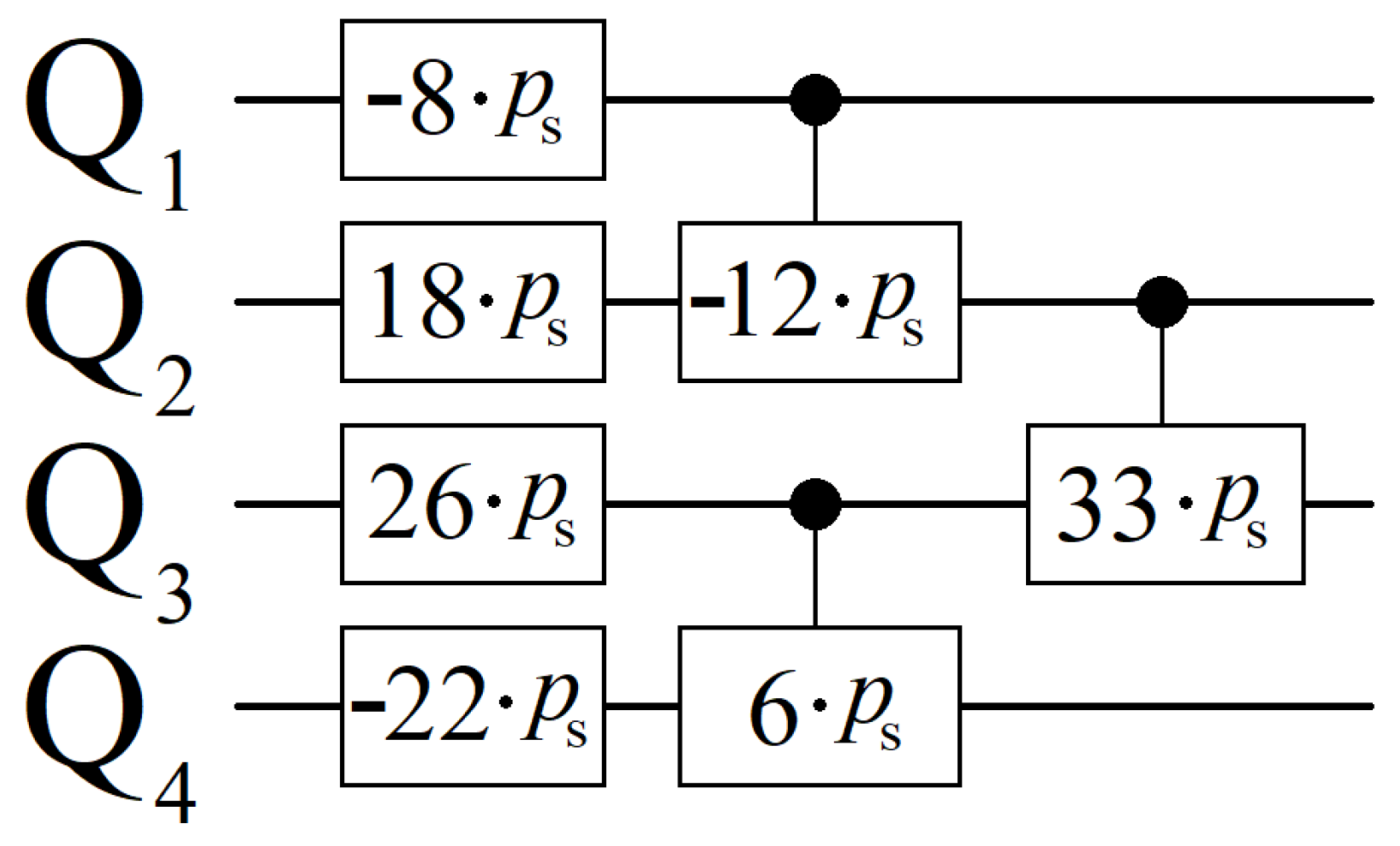
In order to construct such that it is usable for amplitude amplification, a scalar parameter must be included in all of the phase gates. While the value of is problem-specific, its role is always the same: scaling the cumulative phases applied by down (or up) to a range where [C(X), C(X)] is approximately [x, x + ]. This range does not have to be [0, ] exactly, as long as the phases acquired by and are roughly different; see Figure 4 below for an example of in the construction of .
Using the scaled oracle shown in Figure 4 above, we can now show how this new acts on the basis state from before.
As shown in Equation (13) above, multiplying into every phase gate has the net effect of scaling the cumulative phase applied by : e e. Note that this is a global phase, which would have an additive effect on all states rather than a multiplicative one as shown above.
Finding the optimal value for boosting X or X is non-trivial, and was a major focus of our previous study [19] as well as this one. In general, the scale of needed for finding the optimal solution can be obtained using Equation (14) below, which scales the numerical range of a problem [C(X), C(X)] to exactly [x, x + ].
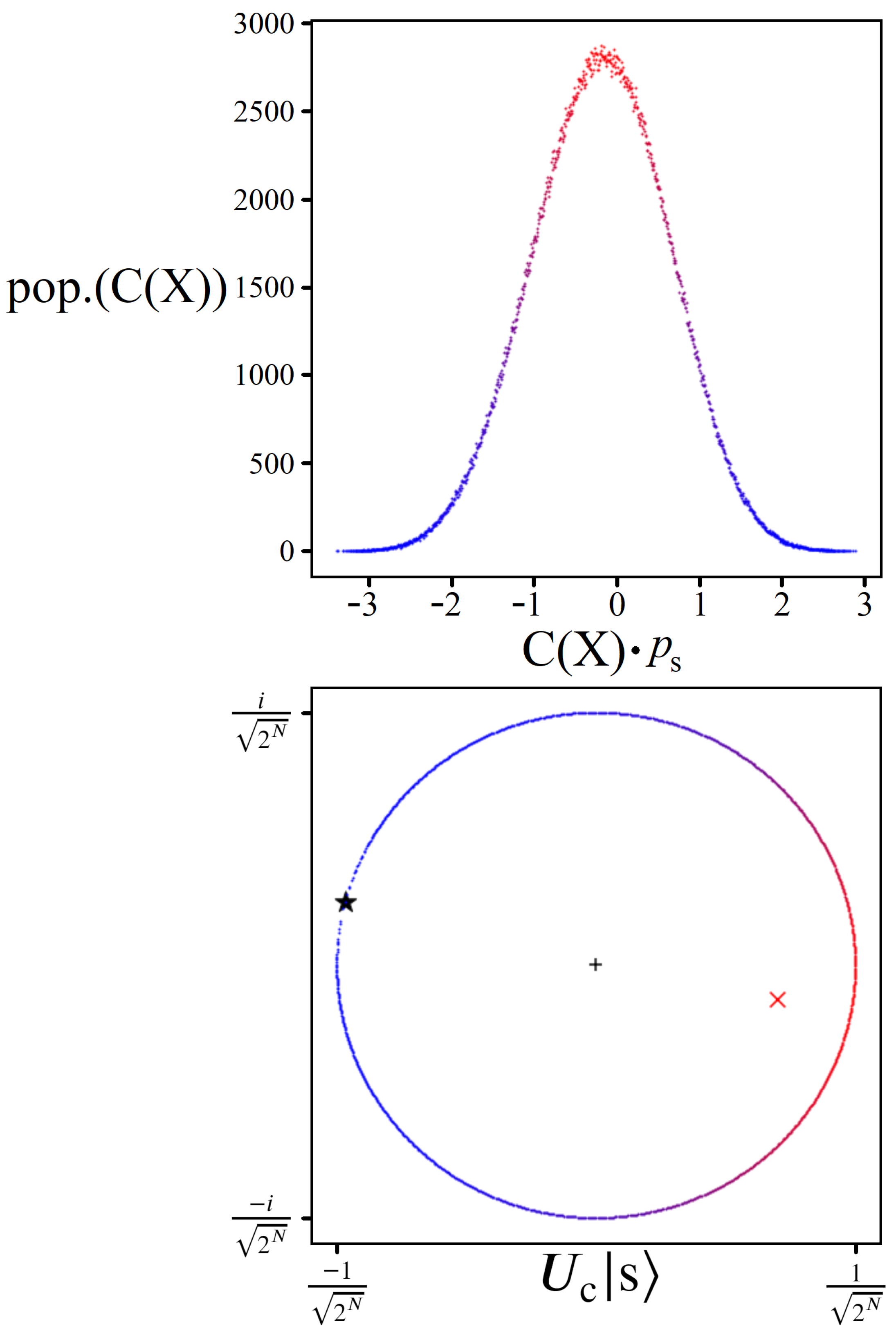
Although Equation (14) above is guaranteed to solve the modulo phase problem mentioned previously, it is almost never the value which can be used to find X or X. Only in the case of a perfectly symmetric solution space distribution is Equation (14) the optimal value, in which case the states and undergo the amplitude amplification process together. However, realistic optimization problems can be assumed to have a certain degree of randomness or asymmetry to their solution space. For this reason, Equation (14) is better thought of as the starting point for finding the true optimal , which we discuss later in Section 4.2. For now, Equation (14) is sufficient for demonstrating the role of in creating an average amplitude suitable for boosting or , as shown in Figure 5.
The bottom plot in Figure 5 shows after the first application of in Algorithm 1. Note the location of the average amplitude (red ‘X′), which is only made possible by the majority of quantum states which recieve phases near the center of the Gaussian in the top plot. The optimal amplitude amplification occurs when the desired state for boosting is exactly phase different with the mean [2,3], which is very close to the situation seen in Figure 5. However, because this is derived from a QUBO with randomized weights, the value provided from Equation (14) does not exactly produce a phase difference between the optimal states (the black star) and the mean amplitude (the red ‘X′). Consequently, the state(s) which become highly probable from amplitude amplification for this particular are not and , which is the subject of the following two sections.
4. Gaussian Amplitude Amplification
The amplitude space plot depicted at the bottom of Figure 5 is useful for visualizing how a Gaussian solution space distribution can be used for boosting; however, the full amplitude amplification process is far more complicated. This is especially true for the QUBOs in this study, which are generated with randomized weights. Consequently, all of the results which follow throughout the remainder of this study are produced from classical simulations of amplitude amplification using cost oracles derived from linear QUBOs according to Equations (1)–(4). For a deeper mathematical insight into these processes, please see [24,25,26].
4.1. Achievable Probabilities
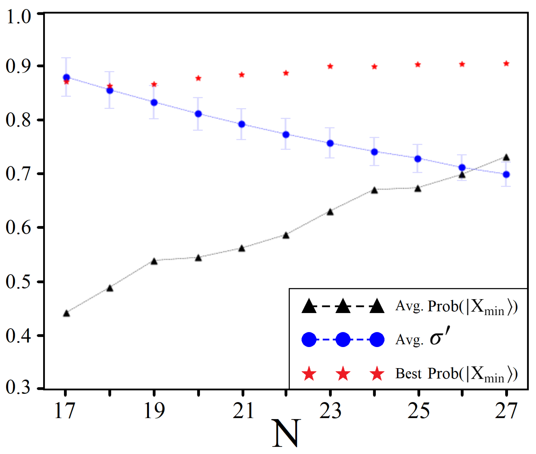
Amplitude amplification is an appealing quantum algorithm because it solves one of the most fundamental problems of quantum computing: measurement probability. For example, a single marked state using Grover’s oracle with 30 qubits is capable of achieving a final probability that is only less than by one billionth of a percent [1]. Thus, a natural question to ask when using is what kinds of probabilities can it produce for or ? To answer this, we conducted a statistical study of linear QUBOs ranging from length to 27. For each N, we generated numerous QUBOs according to Equations (1)–(4), with the totals provided in Appendix A. We then let a classical simulator find the value that maximized the probability of measuring for each QUBO, and for certain cases the optimal for as well. The results for each problem size are shown below in Figure 6.
Figure 6 tracks three noteworthy trends found across the various QUBO sizes: the average peak probability achievable for (the black triangle), the highest recorded probability for (the red star), and the average scaled standard deviation (the blue circle). For clarity, the derivation of is provided by Equations (15)–(17). This quantity is the standard deviation of a QUBO’s solution space distribution after being scaled by , making it a comparable metric for all QUBO sizes. In our previous study, we demonstrated a result in agreement with Figure 6, which is the correlation between higher achievable probabilities for (the red star) and smaller scaled standard deviations (the blue circle) [19]. The latter is responsible for increasing the distance between and the average amplitude, as shown in Figure 5.
4.2. Solution Space Skewness
The relation between N, , and the highest prob.() from Figure 6 can be summarized as follows: larger problem sizes tend to produce smaller standard deviations, which in turn lead to better probabilities produced from amplitude amplification. However, there is a very apparent disconnect between the probabilities capable of each problem size (the red stars) versus the average (the black triangle). To explain this, we must first introduce the quantity X provided in Equation (18) below.
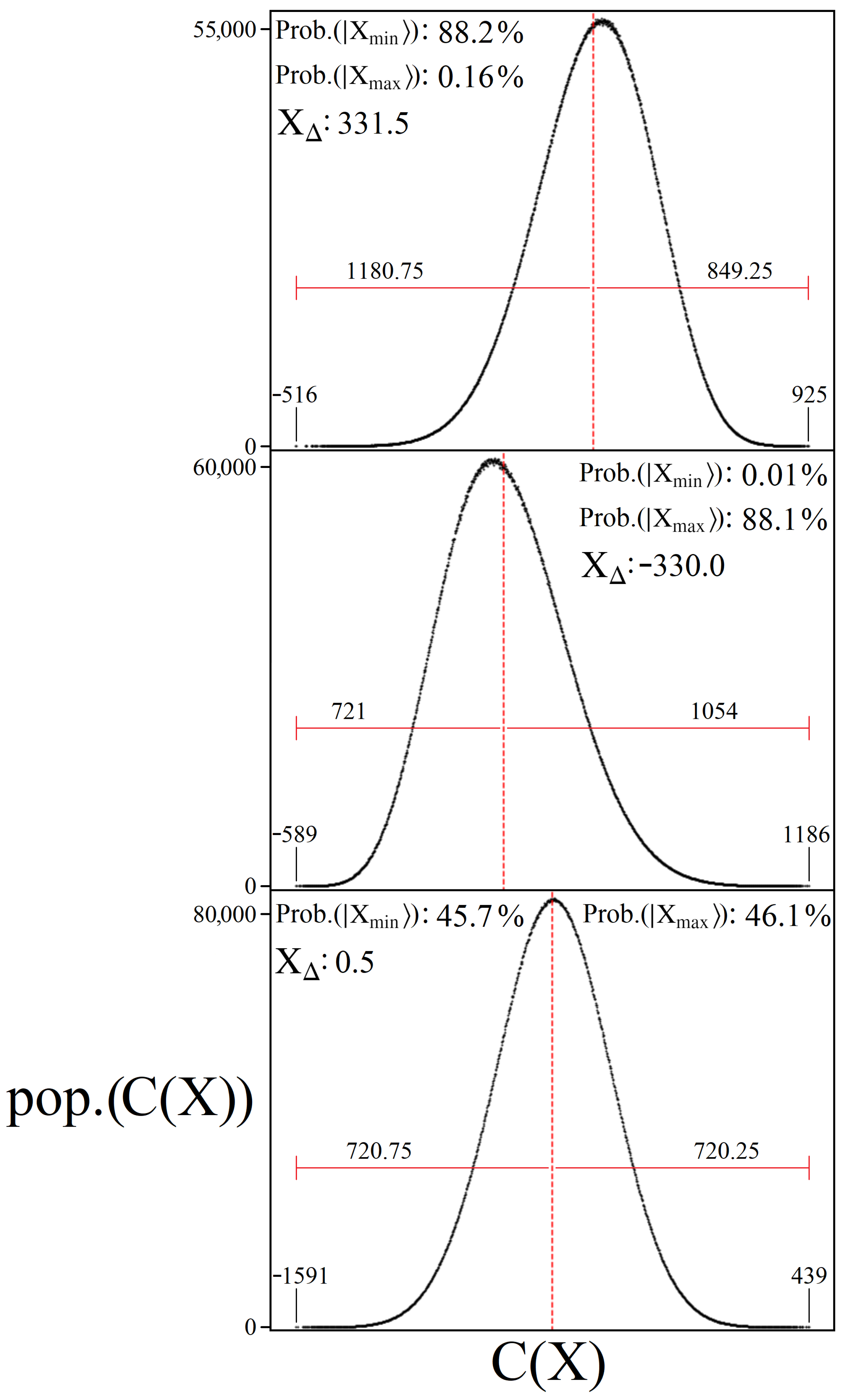
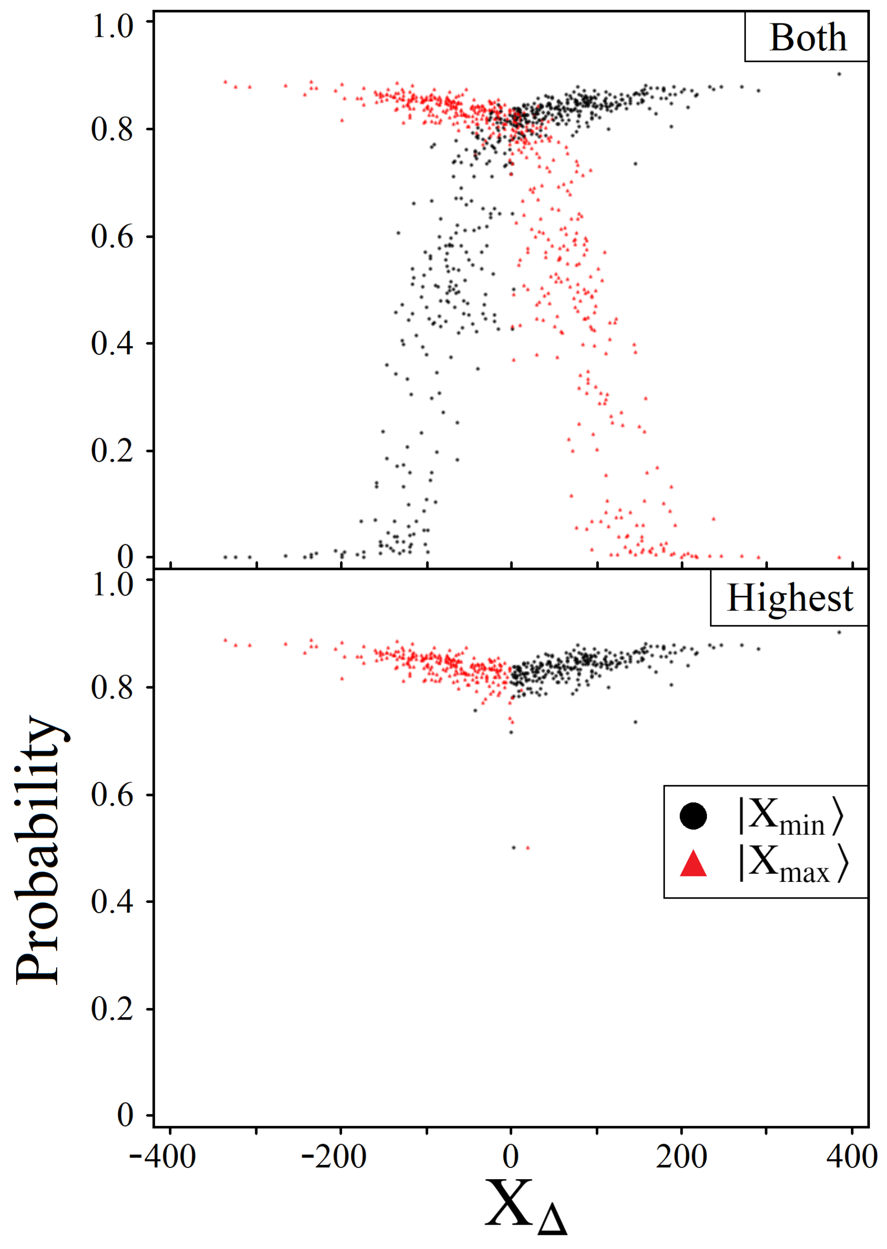
The quantity X from Equation (18) is the difference between and (the mean) minus the difference between and . A positive value for X indicates that the mean is closer to , and vice versa for a negative valued X. In essence, it is a measure of skewness that describes the assymetry of a solution space distribution. Figure 7 shows example QUBO distributions for three cases of X for , demonstrating the impact X has on the ability to boost versus . While is a strong indicator of a problem’s overall aptitude for amplitude amplification, X determines whether or not the optimal minimum or maximum solution is boostable. Further evidence of this can be seen in Figure 8, which shows 1000 randomly generated linear QUBOs of length and the peak probabilities achievable for and as a function of X.
If we compare the average peak probabilites for from Figure 6 with the full data of the QUBOs shown in Figure 8, we can see why the average peak probability is significantly lower than the highest recorded. Across the 1000 QUBOs studied, it is clear that X is a dividing point for whether or is capable of reaching a significant probability of measurement through amplitude amplification. For , the average prob.() reported in Figure 6 is approximately 64%; however, if we instead consider only the QUBOs with X from Figure 8, then the average peak probability for is around 86%, and likewise for when X.
Together, Figure 7 and Figure 8 demonstrate the significance of knowing X from an experimenter’s perspective. Depending on the optimization problem of interest, it is reasonable to assume that an experimenter may be interested in finding only X or only X. Without any a priori knowledge of a problem’s underlying solution space, specifically, X, the experimenter may unknowingly be searching for a solution which is probabilistically near impossible to find through amplitude amplification. For example, considering the QUBO distribution illustrated in the top plot of Figure 7, and the peak probability for boosting : %, although it is ideal to have insight into a particular problem’s X before using amplitude amplification, as we demonstrate in Section 5, information about X can be inferred through measurement results.
4.3. Sampling for
If a particular optimization problem is suitable for amplitude amplification, then the speed of the quantum algorithm outlined in this study is determined by how quickly the optimal value can be found. Here, we show that sampling a cost function C(X) can provide reliable information for approximating from Equation (14), which can then be used to begin the variational approach outlined in 347 s Section 5 and Section 6. Importantly, the number of cost function evaluations needed is significantly less than either a classical or quantum solving speed. The strategy outlined in Equations (19)–(29) below can be used for approximating when the experimenter is expecting an underlying solution space describable by a Gaussian function (Equation (6)). If another type of distribution is expected, then the function used in Equation (22) could in principle be modified accordingly (for example, sinusoidal, polynomial, exponential [26]).
Suppose we sample a particular cost function C(X) M times, where . We define the set as the collection of values C(X) obtained from these samples.
Using these M values, we can compute an approximate mean and standard deviation.
In order to use Equation (14) to obtain , we need approximations for C(X) and C(X). If we assume an underlying Gaussian structure to the problem’s solution space, then we can write the following equation to describe it:
where erf() is the Gaussian error function. Using Equation (24), we can rearrange terms and solve for an approximation to the height of the Gaussian.
With the values , , and obtained from sampling, we can now approximate C(X) and C(X) using Equation (26) below.
Solving for x yields the following two values
which can be expressed in terms of the two quantities originally derived from sampling
Finally, the solutions can be used to obtain .
The reason we set Equation (26) equal to 1 and the integral in Equation (22) equal to is because (x) is modeling the histogram of a QUBO’s solution space, as shown in Figure 2. This means that the total number of solutions to C(X) is , and similarly the minimum number of distinct C(X) solutions for a given cost function is 1. Therefore, after setting the integral in Equation (22) equal to , solving (x) yields approximations for C(X) and C(X) on the tails of the Gaussian.
To demonstrate how well sampling is able to approximate Equation (14), we tested the strategy outlined above against the 1000 QUBOs from Figure 8 (). For four values of M (100, 500, 1000, and 2000), each QUBO was used for 50 trials of random sampling to produce approximate values. These values were then compared to the true value of from Equation (14) as provided by Equation (30) below and finally averaged together to produce Table 1.
The significant result from Table 1 is that sampling 100–500 times on a cost function of solutions is accurate enough to produce an approximate value with an expected error of only 7%. As we show in the next section, this is sufficient accuracy to use for either a heuristic or variational approach for finding optimal solutions.
5. Variational Amplitude Amplification
The results of Section 2, Section 3 and Section 4 demonstrate quantum’s aptitude for encoding and solving a QUBO problem using amplitude amplification. In this section, we discuss how this potential can be realized from an experimental perspective. In particular, we focus on the ability of amplitude amplification to find optimal solutions under realistic circumstances with limited information. The results in this section are then used to motivate Section 6, in which we discuss how amplitude amplification can be used in a hybrid classical–quantum model of computing similar to other successful variational approaches [10,11,12].
5.1. Boosting Near-Optimal Solutions
The results shown in Figure 6, Figure 7 and Figure 8 focus on quantum’s potential for finding and , the optimal solutions which minimize/maximize a given cost function C(X). However, in order to understand how amplitude amplification can be used in a variational model, it is equally as important that non-optimal states are capable of boosting.
As discussed in the conclusion of our previous study [19] as well as in Section 3.3 and Section 4.3, the most difficult aspect of using Algorithm 1 from an experimental standpoint is finding . More specifically, finding an optimal for boosting or is a challenge due to the limited amount of information that can be learned through measurements alone. An example of this can be seen in Figure 9, which shows the peak achievable probabilities of the three lowest states as a function of ( and the next two minimum solutions) for the QUBO corresponding to X from Figure 7.
The challenge presented in Figure 9 is the narrow range of values for which each state is able to achieve meaningful probabilities of measurement. From an experimental perspective, the regions outside these bands are only capable of producing quantum superposition states which are slightly better than , the equal superposition starting state. Thus, an experimenter could use a value that is incredibly close to optimal, but only see seemingly random measurement results through repeat implementations of Algorithm 1.
Our proposed solution to the problem as described above is twofold: (1) we must widen our view of useful values and see where other states become highly probable, and (2) we must place less burden on quantum to find optimal solutions alone when an assisting classical approach may be more suitable. In this section, we focus on addressing (1), which then motivates (2) in Section 6.
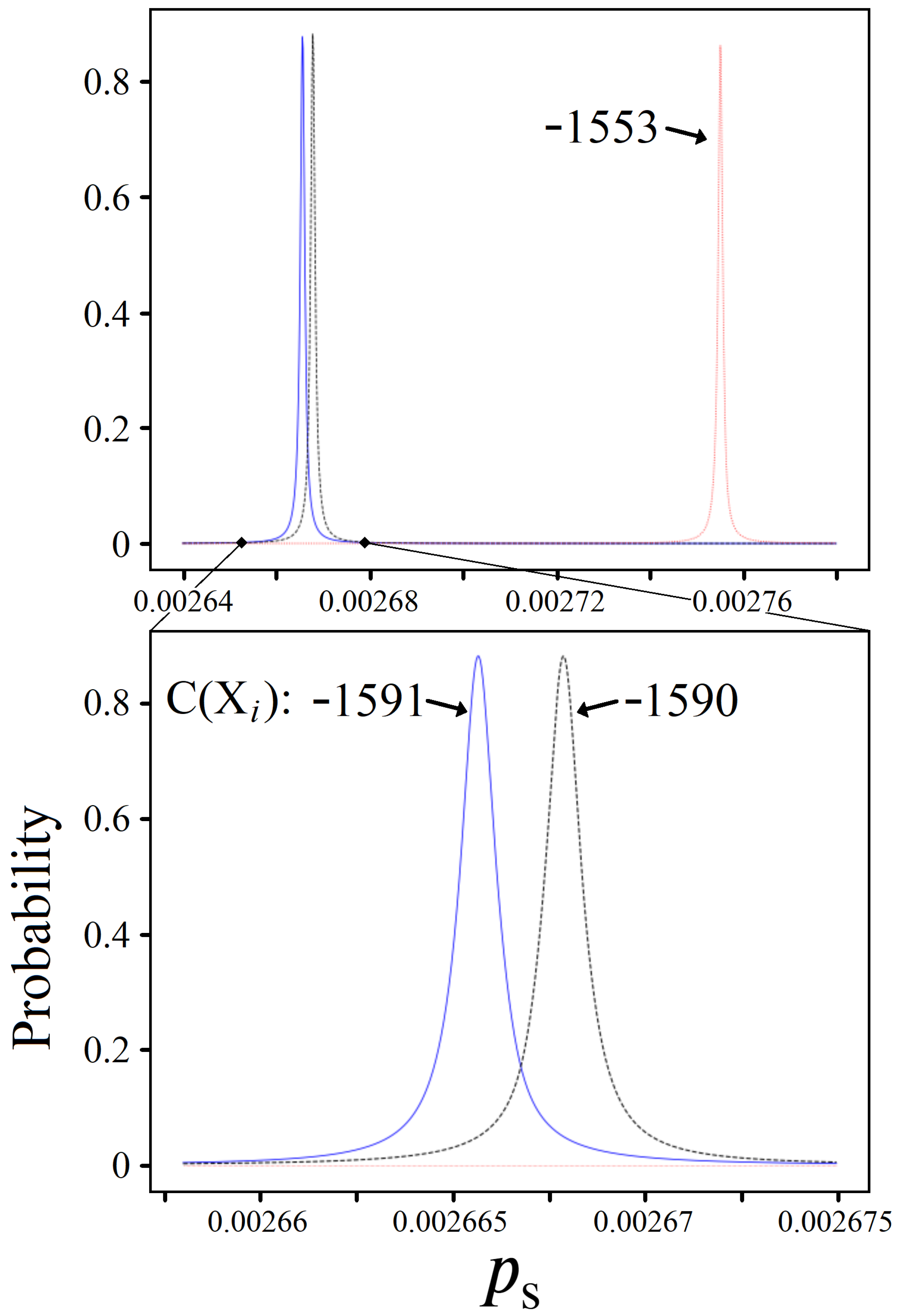
Suppose that we are not solely interested in using quantum to find the exact optimal solution C(X), and instead are content with any X within the best 50 answers (the 50 lowest C(X) values). In order for amplitude amplification to be viable in this heuristic context, it requires significant probabilities of measurement for these non-optimal solution states, similar to Figure 9. Additionally, an experimenter must be able to quickly and reliably find the values which produce them. Shown below in Figure 10 is a plot which provides insight into the feasibility of both of these questions, for the QUBO corresponding to Figure 9.
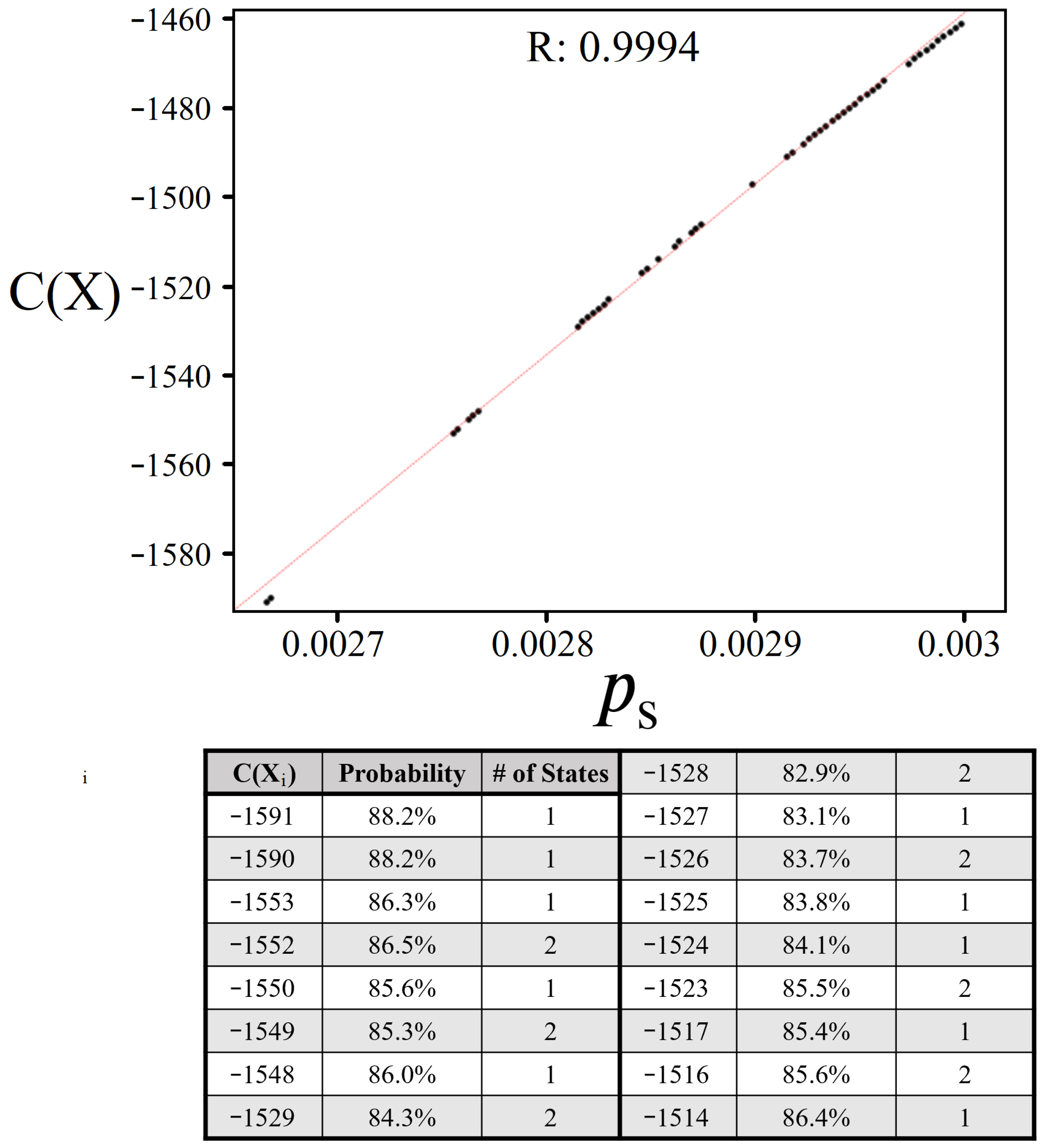
Figure 10 shows the full range for which an experimenter could find the 50 best solutions for minimizing C(X) via quantum measurements. The black circles on the x-axis indicate the values where each state (or multiple states) is maximally probable, aligning with its corresponding C(X) value along the y-axis. Numeric values for peak probabilities of the best 20 solutions are provided in the table below the plot along with a linear regression best fit (the red-dotted line) for the overall 50 data points. The reported R correlation value is provided by Equation (A5) in Appendix B.
There are several significant results displayed in Figure 10, the first of which requires returning to Equation (2). By limiting the allowed weighted values for and to integers, all solutions to C(X) are consequently integers as well. This means that the linear correlation shown in the figure can in principle be used to predict values at which integer C(X) solutions must exist. If and are instead allowed to take on float values, which is more generally the case for realistic optimization problems, the linearity of solutions such as those shown persists, but cannot be used as reliably for predictions of allowed C(X) values.
The linear best fit shown in Figure 10 is accurate for the top 50 solutions; however, extending the scale further reveals that it is only an approximation applicable to a small percentage of states. This is shown in Figure 11 below, which again is a vs. C(X) plot for the same QUBO, except now for the best 400 minimizing solutions. It is clear from the data in this figure that the top 400 solutions are in no way linearly aligned, which is a more expected result considering the complicated nature of these imperfect Gaussian distributions undergoing amplitude amplification. However, although the data are not linear, there is very clearly a curved structure that could be utilized to predict values in the same manner as described above.
It is important to note that in both Figure 10 and Figure 11 the manner in which the solution states are found to be most probable is sequential. This means that if a particular state is most probable at a certain value , then all solutions C(X) < C(X) will have peak probabilities at values . However, the bottom plot in Figure 11 shows that the further a solution state is from , the lower its achievable peak probability; this means that there is a limit to how many solutions are viable for amplitude amplification to find. As we discuss in the coming sections, these are the key underlying features that must be considered when constructing a variational amplitude amplification algorithm.
5.2. Constant Iterations
In order to construct an algorithm which capitalizes on the structure and probabilities shown in Figure 11, we must consider an additional piece of information not illustrated in the figure: step 3 of Algorithm 1, iterations k. The data points in the figure are indeed the values which produce the highest probabilities of measurements; unfortunately, they are achieved using different iteration counts. In principle, this means that an experimenter must decide both and k before each amplitude amplification attempt, further complicating the information learned from measurement results.
Unlike , which is difficult to learn because it depends on the collective solutions to C(X), approximating a good iteration count k is easier. It turns out that the standard number of Grover iterations , where N is the total number of quantum states and M is the number of marked states, is equally applicable when using as well. If an experimenter can use iterations for a cost oracle and find significant probabilities of measurement, then a variational amplitude amplification strategy can be reduced to a single parameter problem: . Figure 12 demonstrates that this is indeed viable, showcasing solution state probabilities as a function of for three different choices of k.
The QUBO corresponding to Figure 12 is the same example for Figure 10 and Figure 11. For instances where multiple states correspond to the same numerical solution (C(X) = C(X)), the solid-color line shown represents their joint probability: prob.( ) + Prob.( ) (note that these individual probabilities are always equal). Examples of this can be seen in the table included in Figure 10. Additionally, a black-dashed line is shown in the top three plots that tracks the collective probability of the five most probable solutions at any given . These three lines are then replotted in the bottom panel for comparison.
The region shown in Figure 12 was chosen to illustrate a scenario where variational amplitude amplification is most viable. For , nearly every possible integer solution C(X) exists via some binary combination for this particular QUBO problem. The exceptions where certain integer solutions do not exist can be seen clearly in the regions with very low probability, for example, . Contrasting this to the region shown in the figure, when becomes closer to where is maximally probable, the measurement probabilities become more akin to Figure 9. Thus, it is more strategic for a hybrid algorithm to start in a region such as in Figure 12, where measurement results can consistently yield useful information.
5.3. Information through Measurements
From an experimental perspective, a significant result from Figure 12 consists of the black-dashed lines shown in the top three plots. At ( for 25 qubits, ), the black-dashed line is almost entirely composed of the single most probable solution state(s). With probabilities around 70–80% for many of the states shown, it is realistic that the same state could be measured twice in only two to four amplitude amplification attempts. Two measurements yielding the same C(X) value (possibly from different X) is a strong experimental indicator that the value used is very close to optimal for that solution, corresponding to the data points from Figure 10 and Figure 11. Confirming three to four different data points in this manner can then be used to approximate the underlying curved structure of these figures, which in turn can be used to predict values where may exist.
While using k closer to is good for getting the maximal probability out of solution states, the and 2000 plots in Figure 12 support a different strategy for quantum. At , the black-dashed line remains primarily composed of the single most probable state(s); critically, however, it does not have the same dips in probability between neighboring solutions. Instead, the cumulative probability stays just as high for these in-between regions, and sometimes even higher! If we now look at the plot, this trend becomes even more prevelant, whereby the cumulative probability plot is on average 20–30% higher than any individual state. Interestingly, the bottom panel of Figure 12 shows that cumulative probability plot for is higher than the line in many regions. Thus, if the role of quantum is to simply provide a heuristic answer, not necessarily , then using lower k values is favorable for a few reasons. First, we can anticipate solutions in a region where multiple states share the same cost function value, and as such can expect more frequently when using . Second, the amplitude amplification process itself is faster due to smaller k, which makes it more achievable on noisy qubits due to shallower circuit depths.
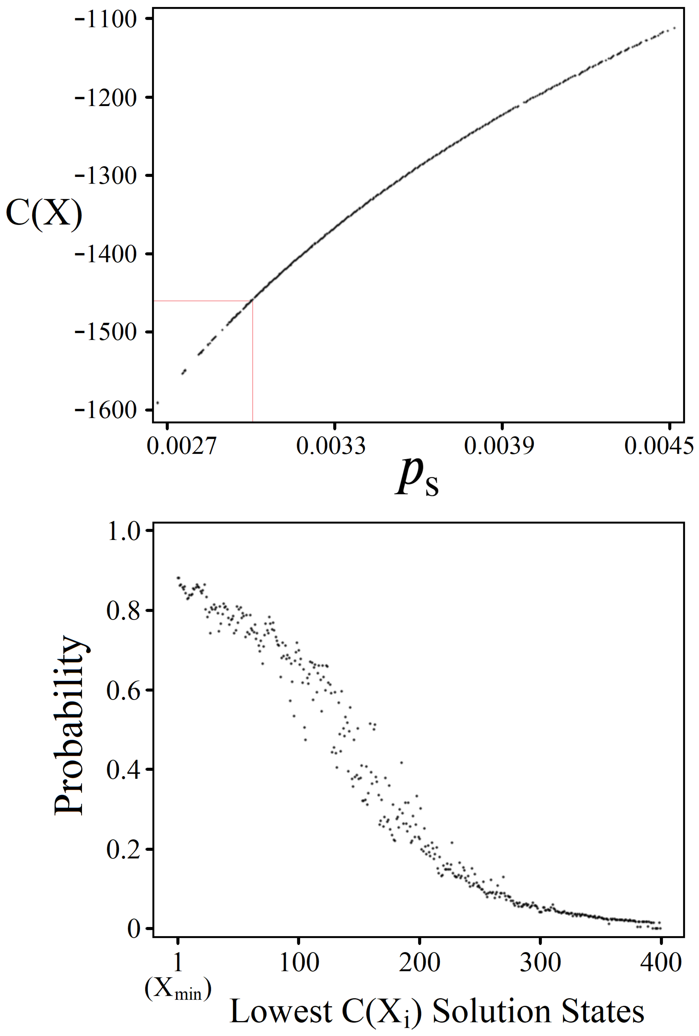
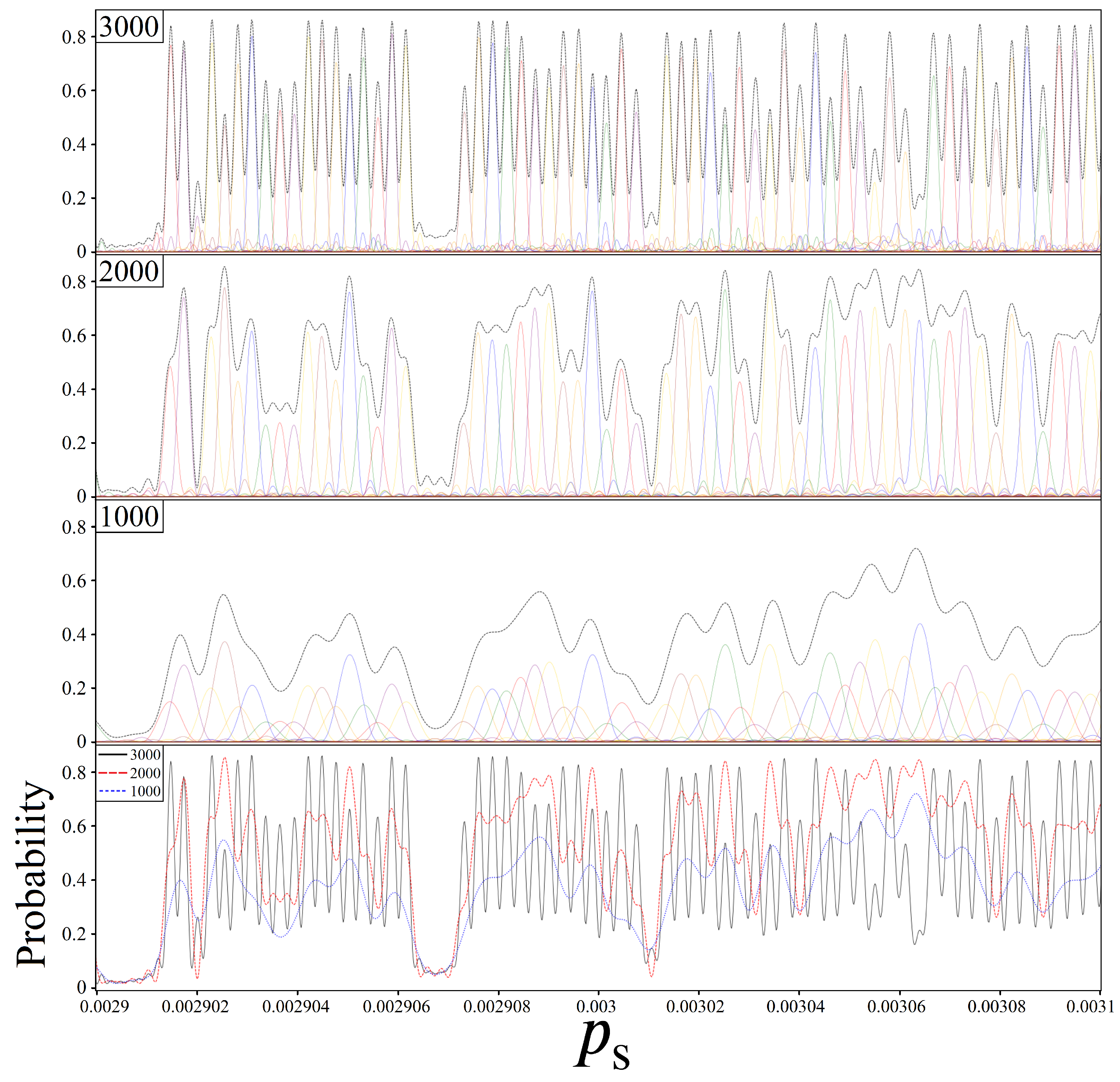
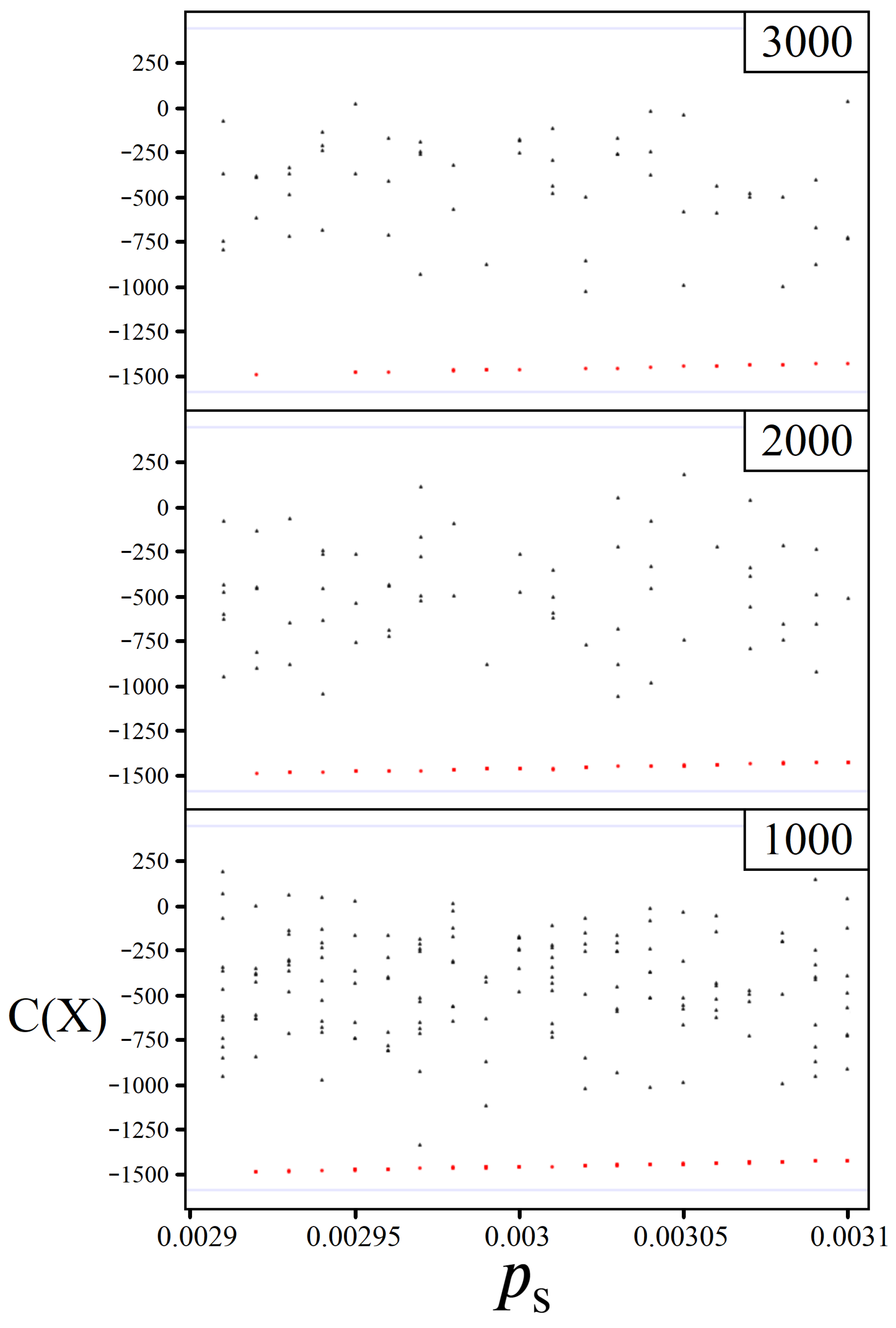
The optimal use of k is a non-trivial challenge to an experimenter. However, as illustrated in Figure 12, amplitude amplification can be effective with a wide range of different k values. To further demonstrate this, Figure 13 shows three plots of simulated measurements over the range depicted in Figure 12. Using the k values 1000, 2000, and 3000, each plot shows data points representing probabilistic measurements at regular intervals of . In order to compare the k value’s effectiveness more equally, the number of measurements taken per value, t, was chosen such that = 12,000 is consistent across all three experiments. Thus, each of the three plots in Figure 13 represents the same total number of amplitude amplification iterations divided among t experimental runs.
The data points shown in Figure 13 are separated into two categories, which are easily recognizable from an experimental perspective. Measurements which yielded C(X) are plotted as red circles, while all other measurements are plotted as black triangles. As illustrated for all three values of k, the red data points can be seen as producing near-linear slopes, all of which would signal to the experimenter that these measurement results are leading to X. The motivation behind Figure 13 is to demonstrate that the same underlying information can be experimentally realized using different k values. Thus, when to use versus is a matter of optimization, which we discuss in Section 6 in the role of a classical optimizer for a hybrid model.
5.4. Quantum Verification
The results of the previous subsections demonstrate the capacity for amplitude amplification as a means of finding a range of optimal X solutions. However, regardless of whether these solutions are found via quantum or classical, a separate problem lies in verifying whether a given solution is truly the global minimum X X. If it is not, then X is referred to as a local minimum. Classically, evolutionary (or genetic) algorithms [37,38,52,53] are one example strategy for overcoming local minima. Similarly, quantum algorithms have demonstrated success in this area for both annealing [54,55] and gate-based approaches [56,57,58].
The strategy for verifying a local versus global minimum using amplitude amplification can be seen by comparing the region in Figure 12 and Figure 13. For the linear QUBO corresponding to these figures, there exists a solution C(X) which becomes maximally probable at , followed by the next lowest solution C(X) at . Because there are no binary combinations X that can produce values C(X) , the region that would correspond to their solutions instead produces nothing measurably significant. This can be seen by the low cumulative probabilities in Figure 12, as well as experimentally in Figure 13 as a gap in the red data points for this region across all three simulations.
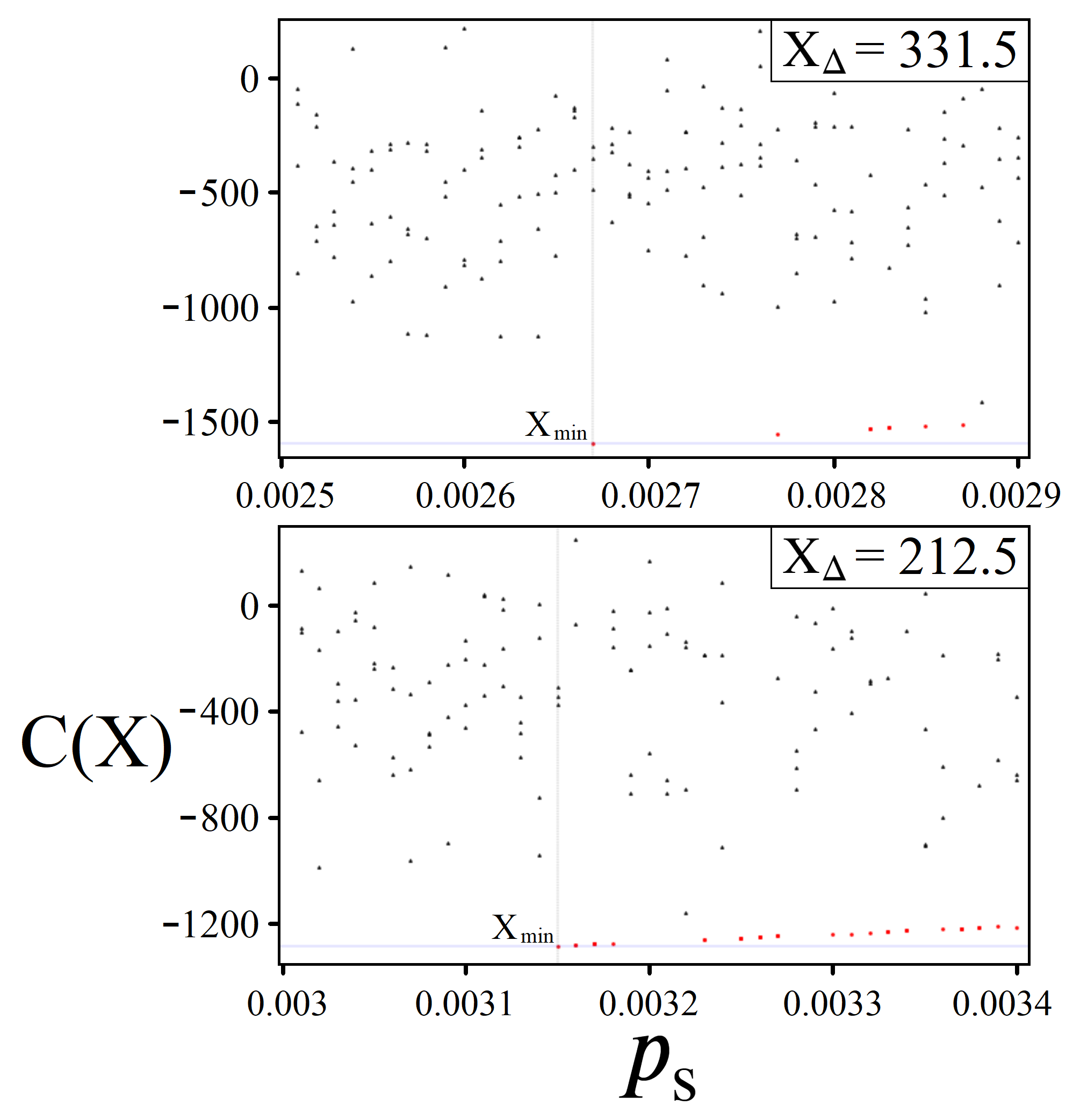
The ability of quantum to determine whether an X solution is a local or global minimum is achieved by searching past the value corresponding to the solution. Doing this results in one of two outcomes: either a lower C(X) value is be found probabilistically, confirming that X was a local minimum, or the experimenter finds only random measurement results, confirming that X was the global minimum. Examples of this can be seen in Figure 14, showcasing simulated measurement results as an experimenter searches past the optimal value for .
The simulated experiments shown in Figure 14 were chosen to highlight both favorable (bottom) and unfavorable (top) cases for quantum. The commonality between both experiments is that there is a clear point in (grey line) in which decreasing any further results in only noisy random measurements. However, determining this cutoff point using measurement results alone is challenging. The top plot corresponds to the QUBO from Figure 10, Figure 11 and Figure 12, which is the non-ideal situation in which there are significant gaps in solutions between the best 20 minimizing C(X). Experimentally, this manifests as numerous regions that could be wrongly interpreted as the X cutoff point. Conversely, the bottom plot represents the ideal case, where the best minimizing C(X) solutions are all closely clustered together. This leads to a much more consistent correlation of measurement results, leading to X, followed by an evident switch to randomness.
The significance here is that amplitude amplification has an experimentally verifiable means for identifying the global minimum X of a cost function. Similarly, the same methodology can in principle be used to check for the existence of an X solution corresponding to any given cost function value, which we discuss further in Section 7.3. However, the obvious drawback is that this verification technique relies on numerous amplitude amplification measurements finding nothing, which costs further runtime as well as being probabilistic. As we discuss in the next section, a more realistic application of this quantum feature is to help steer a classical algorithm past local minima, leaving the verification of X as a joint effort between quantum and classical.
6. Hybrid Solving
The results of Section 5 were all features of amplitude amplification using found through classical simulations of quantum systems. They represent the primary motivation of this study, which is to demonstrate amplitude amplifaction’s potential and the conditions for which it can be experimentally realized. By contrast, the discussions here in Section 6 are more speculative. Considering all of the results from Section 3, Section 4 and Section 5, we now discuss how the strengths and weaknesses of amplitude amplification synergize with a parallel classical computer.
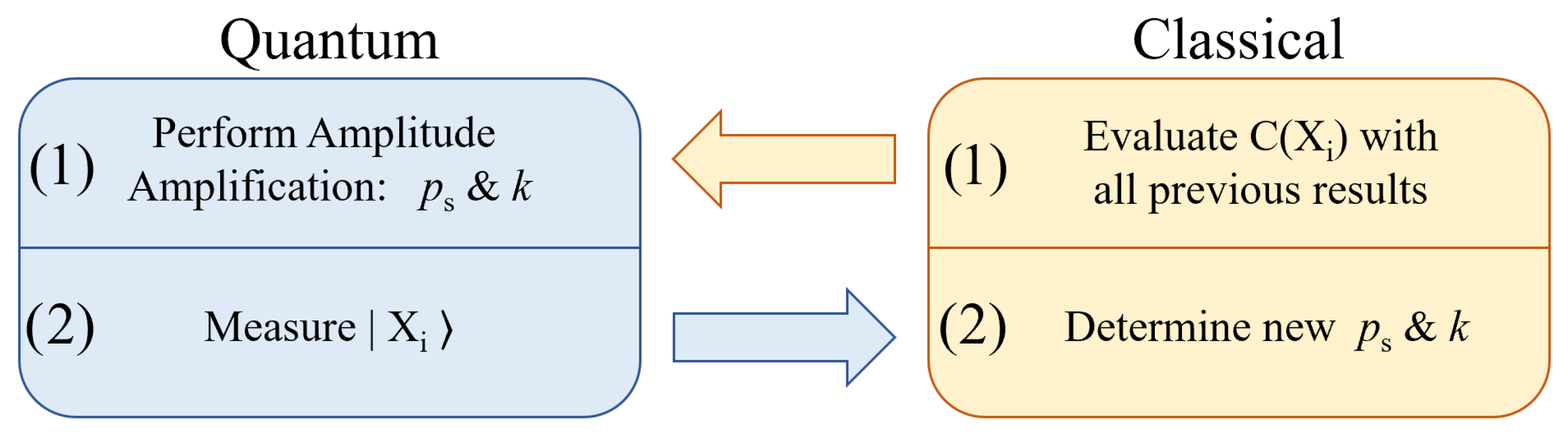
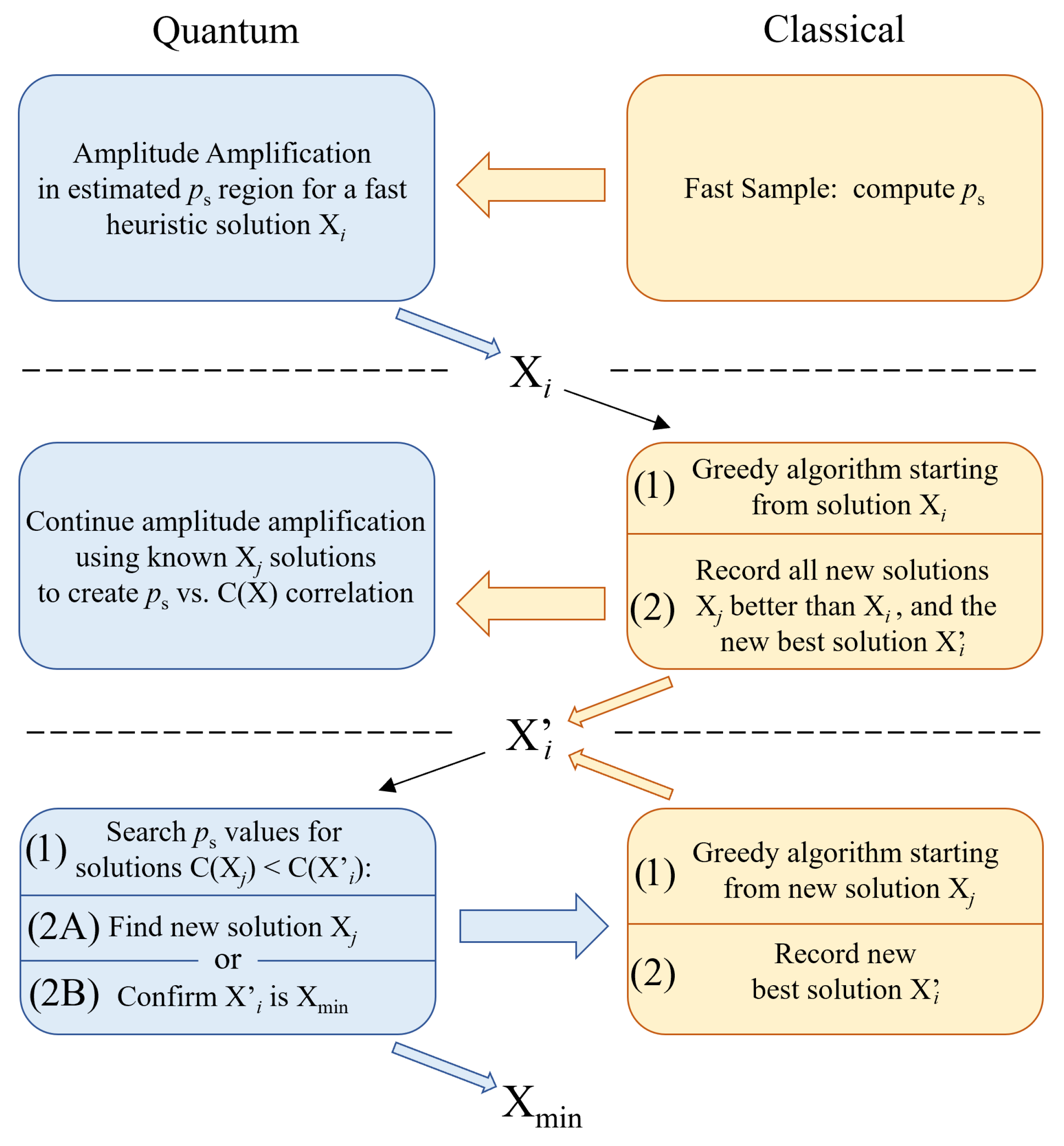
The plots shown in Figure 13 and Figure 14 represent a very non-optimal approach to finding X, functionally a quantum version of an exhaustive search. If the ultimate goal is to solve a cost function problem as quickly as possible, then it is in our best interest to use any and all tools available. This means using a quantum computer when it is advantageous while similarly recognizing when the use of a classical computer is more appropriate. In this section, we discuss this interplay between quantum and classical as well as the situations in which an experimenter may favor one or the other. Shown below in Figure 15 is the general outline of a variational amplitude amplification model which relies solely on quantum to produce X.
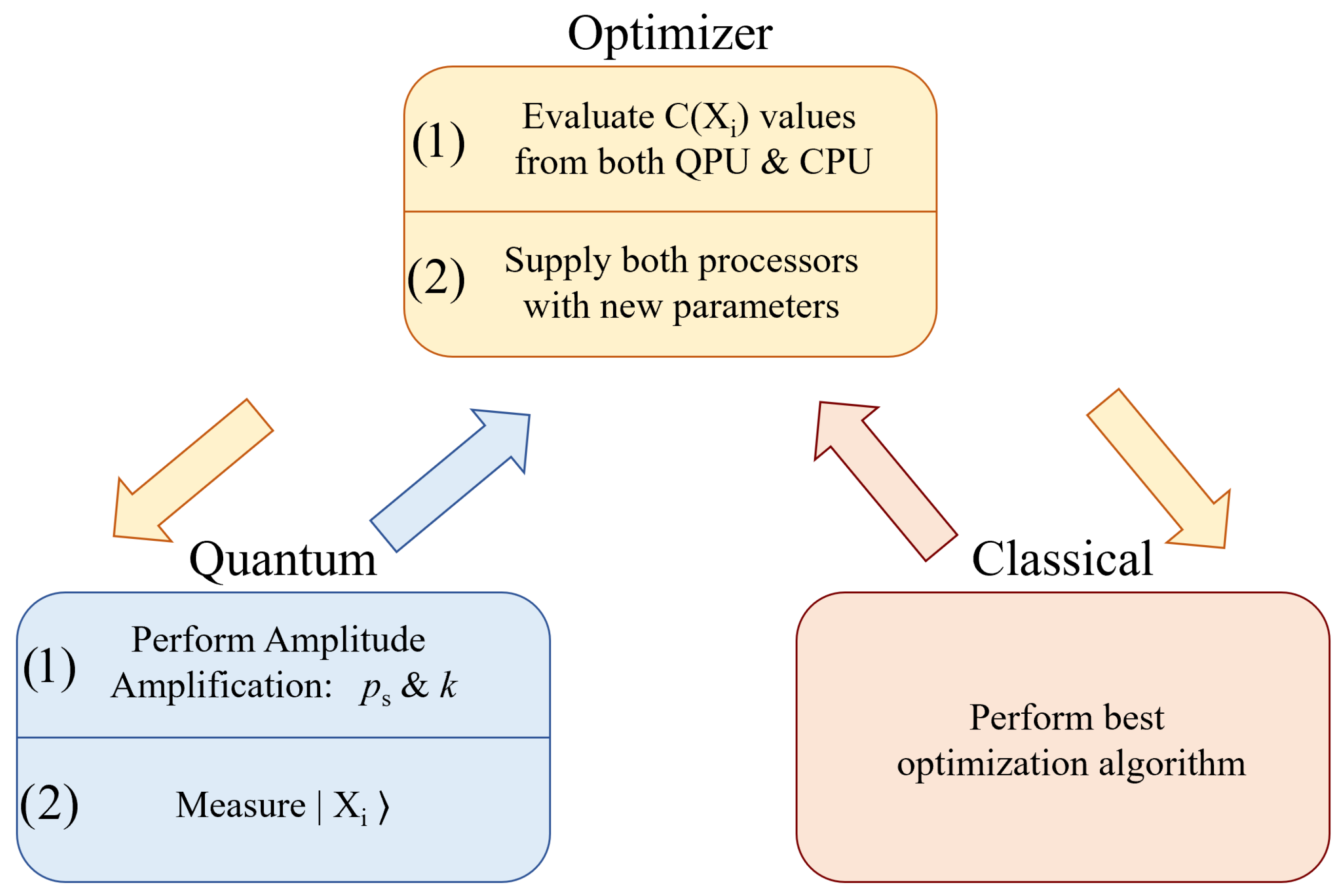
In light of the current state of qubit technologies [59,60,61], performing one complete amplitude amplification circuit should be considered a scarce resource. As such, it is the role of a classical optimizer to determine the most effective use of this resource, choosing and k values which probabilistically lead to the greatest value out of each attempt. Determining optimal values to adjust a quantum circuit is the typical hybrid strategy found among other popular variational models of quantum computing [10,11,12]. The majority of the computational workload is placed on the QPU (quantum processing unit), while a classical optimizer is used in between runs to adjust the quantum circuit parameters accordingly. As evidenced by Figure 13 and Figure 14, this model is possible for amplitude amplification as well. However, there is a different model of hybrid computing which better utilizes both quantum and classical’s strengths, shown below in Figure 16 and Figure 17.
The advantage of hybrid computing using the model shown in Figure 16 is that both processors are working in tandem to solve the same problem utilizing information gained from one another. Information obtained through amplitude amplification measurements can be used to speed up a classical algorithm and vice versa. As we discuss further in the next section, this pairing of quantum and classical is maximally advantageous when the strengths of both computers complement each other’s weaknesses.
Supporting Greedy Algorithms
One notable strength of classical computing is ‘greedy’ algorithms, which provide heuristic solutions for use cases ranging from biology and chemistry [62] to finance [63]. Greedy algorithms are particularly viable for problems that possess certain structures that can be exploited [64]. The key feature to these algorithms is that they focus on making locally optimal decisions that yield the maximal gain towards being optimal. Consequently, while they are very good at finding near-optimal solutions quickly, they are prone to becoming bottlenecked in local minima [65].
The motivation for pairing amplitude amplification with a classical greedy algorithm is best exemplified by Figure 12 and Figure 13. The quantum states illustrated in these figures represent states, which rank as the 30th–80th best minimizing solutions to C(X). Under the right conditions, it is reasonable to expect that a quantum computer could yield a solution in this range within one to five amplitude amplification attempts. The question then becomes how quickly a classical greedy algorithm could achieve the same feat? Without problem-specific structures to exploit, and as problem sizes scale with , it becomes increasingly unlikely that classical can compete heuristically with quantum, which we argue is quantum’s first advantage over classical in a hybrid model.
Now, supposing that amplitude amplification does yield a low C(X) solution faster than classical, the problem then flips back to being classically advantageous. This is because the X solution provided by quantum is now new information available to the classical greedy algorithm. As such, beginning the greedy approach from this new binary string is likely to yield even lower C(X) solutions in a time frame faster than amplitude amplification. For example, this is the exact scenario in which genetic algorithms shine [37,38,52,53,63], where a near-optimal solution is provided from which they can manipulate and produce more solutions. If a fast heuristic solution is all that is needed, then quantum’s job is done, and the best minimal solution found by the classical greedy algorithm completes the hybrid computation.
However, if a heuristic solution is not enough then we can continue to use a hybrid quantum–classical strategy to find X. Referring back now to Figure 13 and Figure 14, the strategy for quantum is to use multiple amplitude amplification trials and measurements to approximate the underlying correlation from Figure 10 and Figure 11. The fastest means of achieving this is to work in a region analogous to Figure 12, where one has the highest probabilities of measuring useful information experimentally. Simultaneously, the classical greedy algorithm can find X solutions in this area as it searches for X. Knowledge of these X solutions can be directly fed back to quantum, which can be used to predict values where solutions are known to exist, speeding up the process of determining a vs. C(X) correlation. Thus, after quantum initially aids classical, subsequent information obtained from classical can then be used to speed up quantum.
In the time it takes for quantum to experimentally verify enough and C(X) values to create a predictive correlation, we expect the classical algorithm to find a new lowest C(X) solution, which is labeled as X′ in Figure 17. After investing additional trials into the amplitude amplification side of the computation, it is now time for quantum’s second advantage: verifying local versus global minima. Using an approximate vs C(X) best fit, the quantum computer can skip directly to the value corresponding to best currently known X′ solution. As discussed in Section 5.4, searching past this value results in one of two outcomes: either the quantum computer finds a new best solution C(X) < C(X′), or it confirms that X′ is indeed the global minimum X. In the former case, the greedy algorithm now starts again from the new lowest solution X, repeating this cycle between quantum and classical until X is found. Figure 17 below shows a workflow outline of this hybrid strategy.
The biggest advantage of using a hybrid model such as the one shown in Figure 17 is that it can be adapted to each problem’s uniqueness. Problems with known fast heuristic techniques can lean on the classical side of the computation more heavily [66,67], while classically difficult problems can place more reliance on quantum [68,69]. Above all, this model of computation incorporates and synergizes the best known classical algorithms with quantum rather than competing against them.
7. More Oracle Problems
All of the results from Section 3, Section 4 and Section 5 were derived from linear QUBOs according to Equations (1)–(4). However, these results can be applied to more challenging and realistic optimization problems provided that (1) all possible solutions can be encoded via phases by an appropriate oracle operation and (2) the distribution of all possible answers is suitable for boosting the solution we seek (Gaussian, polynomial, exponential, etc. [26]). Here, we briefly note a few additional optimization problems which meet both of these criteria.
7.1. Weighted and Unweighted Max-Cut
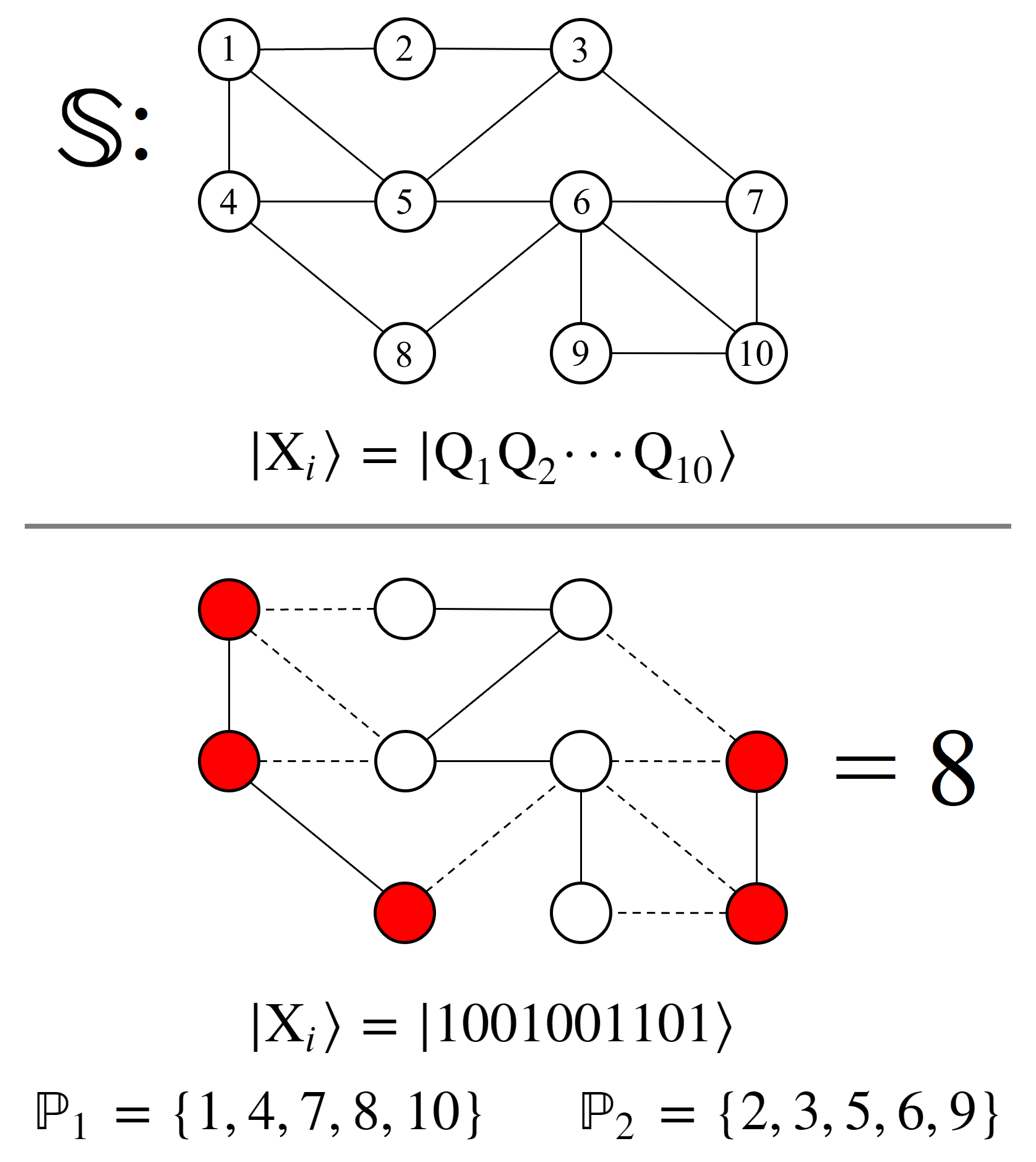
The Maximum Cut problem (‘Max-Cut’) is famously NP-Hard [68], where the objective is to partition every vertex in a graph into two subsets and such that the number of edges between them is maximized. In the weighted Max-Cut version of the problem, each edge is assigned a weight and the goal is to maximize the sum of the weights contained on edges between and . The unweighted Max-Cut problem has already been demonstrated as a viable use for amplitude amplification [25], which we build upon further here via the weighted version. Equation (31) below is the cost function C(X) for the weighted Max-Cut problem, which can be converted to the unweighted case by setting every edge weight . The binary variables here represent being partitioned into or .
Shown in Figure 18 is an example graph and one of its solutions. This example graph is composed of 10 vertices, labeled 1–10, and a total of 15 connecting edges. Encoding this graph requires one qubit per vertex, where the basis states and represent belonging to the subsets and , respectively. See the bottom graph in Figure 18 for an example solution state.
The cost oracle for solving Max-Cut must correctly evaluate all solution states based on the edges of according to Equation (31). For example, if vertices 1 and 2 are partitioned into different sets, then needs to affect their combined states and with the correct phase, either weighted or unweighted. Just as in Figure 3 from earlier, we can achieve this with a control-phase gate CP(), with the intent of scaling by later (see Figure 4). The caveat here is that we need this phase on and , not , which means that additional X gates are required for the construction of , as shown below in Equation (32).
For the complete quantum circuit which encodes the graph in Figure 18, please see Appendix C. When properly scaled by , the solutions that are capable of boosting are determined by the underlying solution space distribution of the problem, which can be seen in Figure 19 below. The histogram in this figure shows all C(X) solutions to the graph from Figure 18. Even for a 10 qubit problem size such as this, it is clear that the underlying solution space distribution shows a Gaussian-like structure.
One interesting feature of Max-Cut is that all solutions come in equal and opposite pairs. For example, the optimal solutions to from Figure 19 are and , which both yield 13 ‘cuts’. Mathematically, there is no difference between swapping all vertices in and , while physically it means that there are always two optimal solution states. Consequently, these states always share the effect of amplitude amplification together, which is something that an experimenter must be aware of when choosing iterations k.
Finally, moving from the unweighted to the weighted version of Max-Cut increases the problem’s difficulty, though it notably does not change the circuit depth of . Rather than using for all of the control-phase gates, each now corresponds to a weighted edge of the graph. Similar to the QUBO distributions shown in Figure 7, this increase in complexity allows for more distinct C(X) solutions, and consequently more variance in features such as and X.
7.2. Graph Coloring
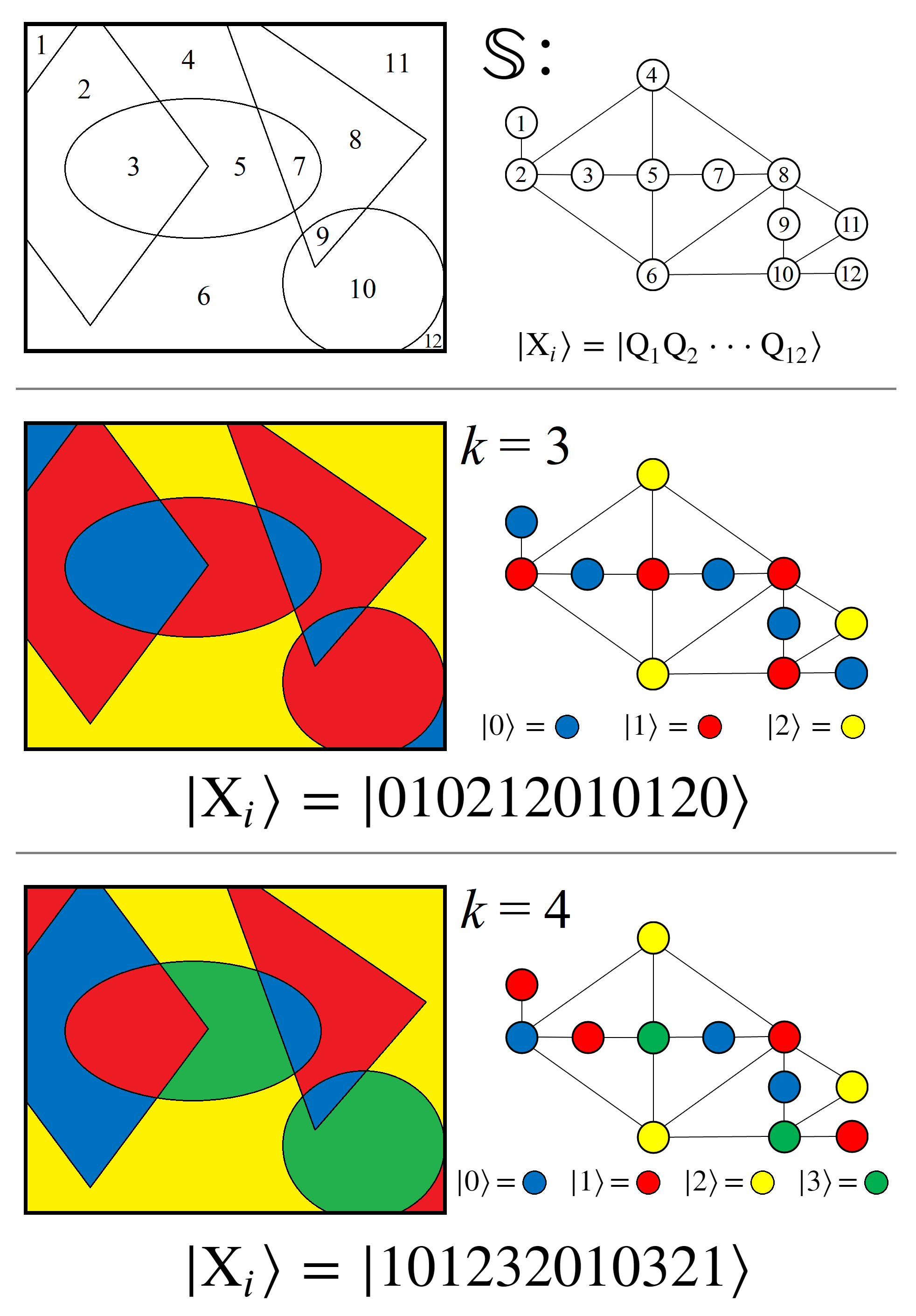
A similar optimization problem to Max-Cut is Graph Coloring, sometimes known as Vertex Coloring [68], which extends the number of allowed partition sets up to any integer number k ( is equivalent to Max-Cut). For a given graph of vertices and edges , the goal is to assign every vertex to a set such that the number of edges between vertices within the same sets is minimized. Shown below in Equation (33) is the cost function C(X) for a k-coloring problem, where the values of each vertex are no longer binary and can take on k different integer values. The quantity inside the parentheses is equal to 1 if and 0 for all other combinations . Just as with Max-Cut, setting all is the unweighted version of the problem.
The name ‘coloring’ is in reference to the problem’s origins, whereby the sets all represent different colors to be applied to a diagram, such as a map. Shown below in Figure 20 is an example picture composed of overlapping shapes, where each section must be assigned one of k colors such that the number of adjacent sections with the same color is minimized. Example solutions for and are shown along with their vertex and quantum state representations of the problem.
In order to encode graph coloring as an oracle , the choice of k determines whether qubits or another form of quantum computational unit is appropriate. While qubits are capable of producing superposition between two quantum states, qudits are the generalized unit of quantum information capable of achieving superposition between d states [70,71,72,73]. To see why this is necessary, let us compare the and 4 examples from Figure 20 and the quantum states needed to represent partitioning each vertex.
For , we need four distinct quantum states to represent a vertex belonging to one of the partitions. While a single qubit cannot do this, a pair of qubits can. Thus, every vertex in can be encoded as a pair of qubits, letting the basis states , , , and each represent a different color. Alternatively, we could use a qudit to represent each vertex, assigning each partition a unique basis state: , , , or , such as the state shown in Figure 20. Mathematically, the two encodings are identical; thus, the choice of whether to use qubits or qudits is a matter of experimental realization, i.e., which technology is easier to implement.
For however, two qubits is too many states, while a single qubit is not enough. Thus, in order to represent three colors exactly in quantum, the appropriate unit is a ‘qutrit’ (the common name for a qudit). Similarly, all prime numbers d can only be encoded as their respective d-qudits, while all composite values can be built up from combinations of smaller qudits. When an appropriate mixed-qudit quantum system is determined, constructing is the same as the Max-Cut problem from earlier, now with k state–state interactions. For an example of qudit quantum circuits and their use for amplitude amplification, please see Wang et al. [70] and our previous work on the Traveling Salesman problem [19].
7.3. Subset Sum
For all of the oracles discussed previously, the circuit depth and total gate count for are determined by the size and connection complexity of , i.e, the graphical representation of the problem. By contrast, the simplest possible quantum circuit that can be used as corresponds to the Subset Sum problem [68]. The cost function for this problem is provided in Equation (34).
Rather than optimizing Equation (34), which is trivial, in the Subset Sum problem we seek to determine whether there exists a particular combination such that C(X) = T, where T is some target sum value. The boolean variables represent which values to use as contributors to the sum. Figure 21 below shows an example. Note that this problem is equally applicable to any of the other oracles discussed previously, whereby we can ask whether a target value T exists for some graph .
The reason why Equation (34) is the simplest oracle that can be constructed is because the cost function does not contain any weights that depend on two variables. Consequently, the construction of does not use any 2-qubit phase gates CP(), instead only requiring a single qubit phase gate P() for every qubit. In principle, all of these single qubit operations can be applied in parallel, such as in Figure 3, which means that the circuit depth of is exactly one.
Although this is the most gate-efficient , using it to solve the Subset Sum problem comes with limitations. First, it can only solve for T values within a limited range. This is illustrated by the results of Figure 11, which demonstrate that amplitude amplification can only produce meaningful probabilities of measurement up to a certain threshold away from X or X. Consequently, it is only possible to use here if the target sum value T is within this threshold distance from the extrema.
The second limitation to consider is the discussion from Section 5.4, whereby the information about whether or not a state C(X) exists may rely on measurements finding nothing. Previously, we discussed how an experimenter might iteratively decrease and eventually expect to find regions where cost function values do not exist (see Figure 14) as one approaches X. Here, things are easier, as an experimenter can test for values above and below where C(X) (except for the case where T is the global extremum). Using a vs. C(X) correlation in this manner can confirm exactly where the value for C(X) must be. Testing this window then either confirms the existence of a solution for T via measurement, or conversely confirms no solution exists through multiple trials of random measurement results.
8. Conclusions
The results of this study demonstrate that the gate-based model of amplitude amplification is a viable means of solving combinatorial optimization problems, particularly QUBOs (though beyond QUBOs as well; see Section 7). The ability to encode information via phases and let the superposition of qubits naturally produce all possible combinations is a feature entirely unique to quantum. Harnessing this ability into a useful algorithmic form was the primary motivation for this study, and as we have shown, is not without its own set of challenges. In particular, the discussions in Section 4.1 and Section 4.2 highlight that this algorithm is not a ‘one size fits all’ strategy that can be blindly applied to any QUBO. Depending on how the numerical values of a given problem form a solution space distribution, it may simply be impossible for amplitude amplification to find one extremum or the other. Figure 8 shows that at least one of the extremum solutions for quantum to find is always viable, though this may not be the one that is of interest to the experimenter.
For cases where the desired solution is well-suited for quantum to find, that is, the desired or is capable of achieving a high probability of measurement, a different challenge lies in finding the correct value to use in order to boost these states. However, the results in Section 5 illustrate that this challenge is solvable via quantum measurement results. If the best an experimenter could do is simply to guess at and hope for success, then amplitude amplification would not be a practical algorithm. However, the correlations shown in Figure 10 and Figure 11 illustrate that this is not the case, and that information about can be experimentally learned and used to find extremum solutions. How quickly this information can be experimentally produced, analyzed, and used is exactly how quickly quantum can find the optimal solution, which is an open question for further research.
Regarding the scalability of the amplitude amplification and the future potential of the approach laid out in this study, there are three important results to address. First, the quantum circuit encoding of combinatorial optimization problems such as QUBOs can be seen to have high circuit depth efficiency, as shown in Figure 3 and Figure 4. Requiring only a two-qubit control phase is significantly more NISQ-friendly than other proposed oracles, which often require full N-qubit control operations to mark states. Next, Figure 6 demonstrates that amplitude amplification performs better mathematically at higher qubit sizes. The underlying reason for this can be seen in Figure 5, where increasing qubit size leads to more superposition states, pulling the mean point phase away from suitable states for boosting. However, the major challenge of scaling up this approach, aside from the noise and decoherence which plague all quantum algorithms, is higher demand on phase control via the free parameter . Our proposed cost oracles require phases across all superposition states, which are always constrained to a range of approximately . Thus, as the problem size increases, the precision required by does as well.
While the free parameter can be considered the bottleneck of our algorithm for finding the global optimal solution (Figure 9), it unlocks a different use case for amplitude amplification, namely, as a heuristic algorithm. A major finding of this study is depicted in Figure 11 and Figure 12, which show that there is a wide range of values for which quantum can find an answer within the best 1–5% of all solutions. As demonstrated with sampling in Section 4.3, it is not unrealistic that a classical computation can estimate this region very quickly. The question then becomes how this quantum heuristic approach, which is O(), compares to classical greedy algorithms in terms of both speed and accuracy. Additionally, a fast quantum heuristic solution is equally beneficial for a classical computer, whereby the information learned through quantum measurements can be of equal use to speed up a classical algorithm as well. Understanding which optimization problems this scenario may be applicable to is the future direction of our research.
Author Contributions
Conceptualization, D.K. and M.C.; Formal analysis, D.K.; Investigation, M.C., S.P. and P.M.A.; Resources, L.W.; Supervision, P.M.A.; Project administration, L.W. All authors have read and agreed to the published version of the manuscript.
Funding
This research received no external funding.
Data Availability Statement
The data and code files that support the findings of this study are available from the corresponding author upon reasonable request.
Acknowledgments
Any opinions, findings, conclusions, or recommendations expressed in this material are those of the author(s) and do not necessarily reflect the views of AFRL.
Conflicts of Interest
The authors declare no conflict of interest.
Appendix A. QUBO Data
For this study, linear QUBOs as defined in Equation (4) were created using a uniform random number generator for node and edge weights according to Equations (2) and (3). The total number of QUBOs produced and analyzed to create Figure 6 is provided below in Table A1. Every QUBO was simulated through amplitude amplification, and the value which yielded the highest probability of measurement for was recorded.

Table A1.
Table of values showing the number of linear QUBOs generated and studied per size N.
| # of QUBOs Studied | |
|---|---|
| 17 | 5000 |
| 18 | 3000 |
| 19 | 2000 |
| 20 | 1500 |
| 21 | 1200 |
| 22 | 1000 |
| 23 | 1000 |
| 24 | 600 |
| 25 | 500 |
| 26 | 400 |
| 27 | 100 |
Appendix B. Linear Regression
In order to determine how linearly correlated the data points in Figure 10 were, a regression best fit was performed according to Equations (A1)–(A5) below. The collection of (x,y) data points D in Equation (A1) corresponds to the (,C(X)) points in the figure. The resulting linear correlation factor R is reported at the top of Figure 10.
Appendix C. Max-Cut Circuit
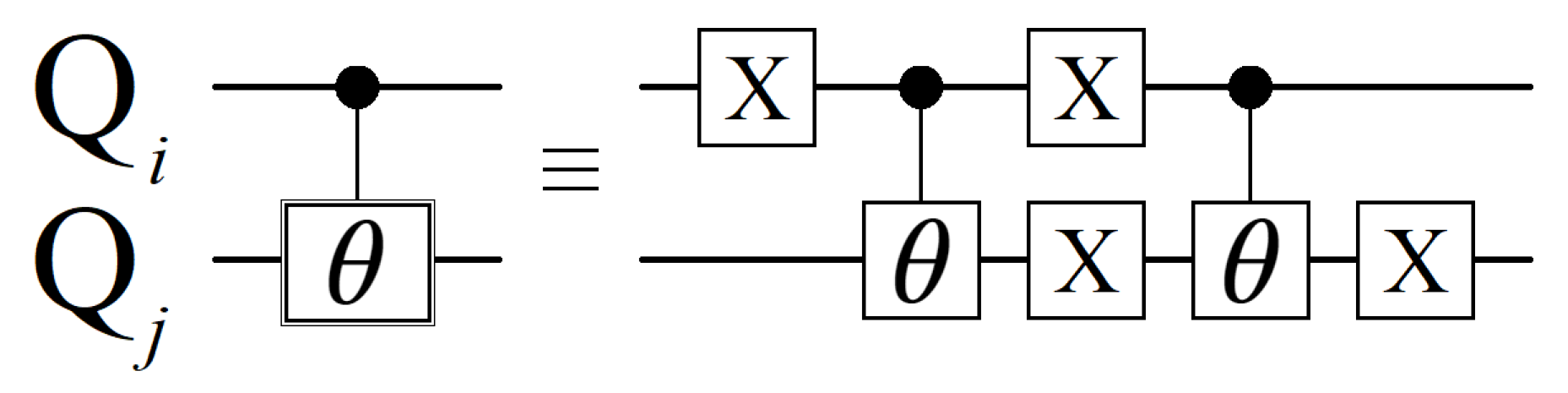
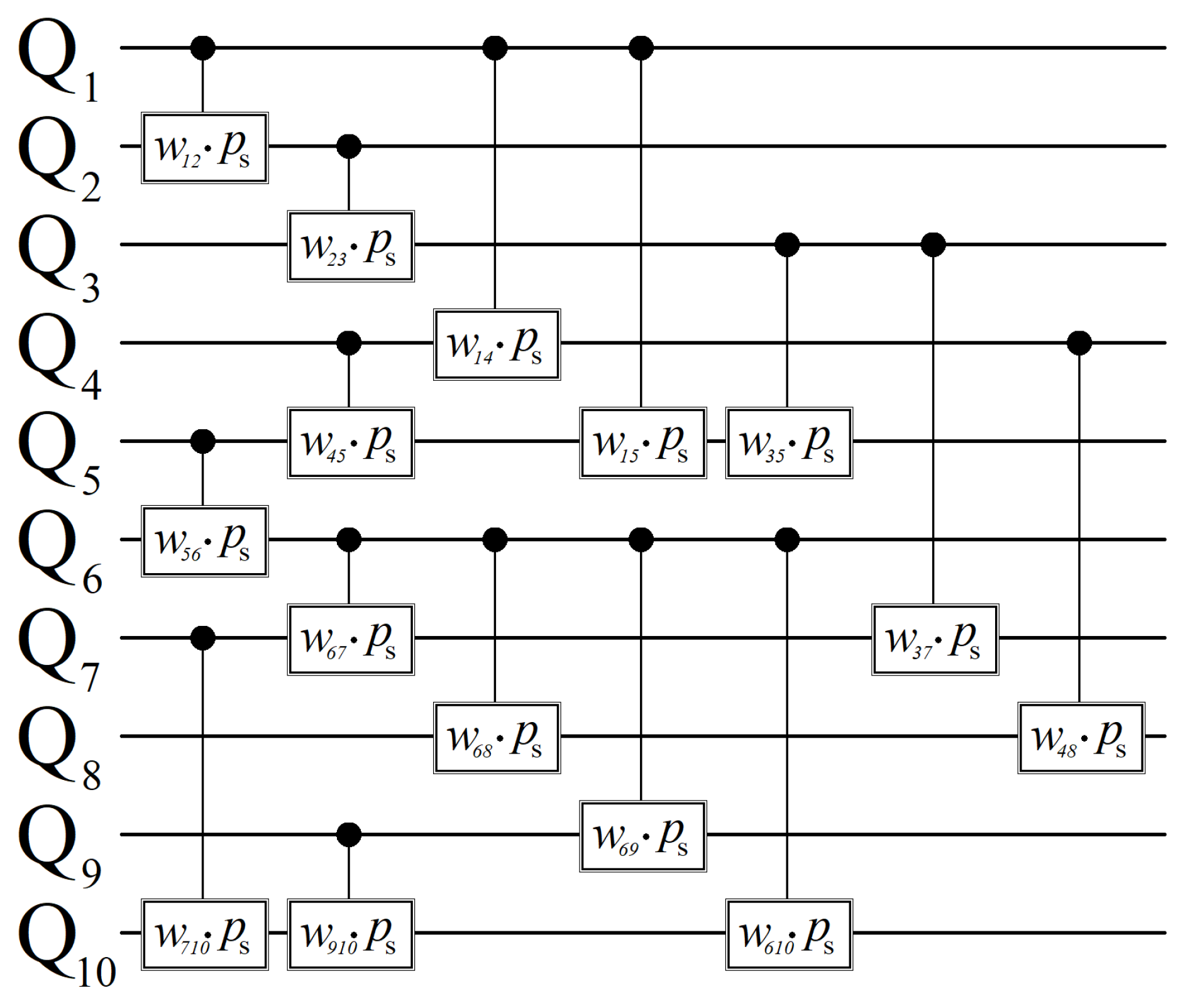
To illustrate how any graph structure can be encoded as an oracle , Figure A2 below shows the quantum circuit corresponding to from Figure 18. Because this oracle needs to represent a Max-Cut problem (weighted or unweighted), the states which must acquire phases are and . To make the circuit less cluttered, we can define the custom gate shown in Figure A1.
Figure A1.
Quantum circuit which achieves the 2-qubit unitary from Equation (A6).
Figure A1.
Quantum circuit which achieves the 2-qubit unitary from Equation (A6).

The quantum circuit shown in Figure A1, drawn similar to a CP() gate with an extra box around it, is an operation which achieves the following unitary:
The unitary U from Equation (A6) is the required operation for representing the cost oracle in Equation (31). If two nodes (qubits) share a connection in , then a ‘cut’ corresponds to them being partitioned into different sets, which is represented by the qubit states and . Figure A2 uses the operation in Figure A1 to create the complete circuit for encoding all 15 connections in .
Figure A2.
Quantum circuit which achieves the oracle corresponding to from Figure 18, for the Max-Cut problem. Each gate shown here represents one of the 15 connections in , corresponding to the custom gate defined in Figure A1. The placement of gates shown here has them spread out for clarity; a real implementation could be more parallelized.

References
- Grover, L.K. A fast quantum mechanical algorithm for database search. arXiv 1996, arXiv:9605043. [Google Scholar]
- Boyer, M.; Brassard, G.; Hoyer, P.; Tapp, A. Tight bounds on quantum searching. Fortschritte Phys. 1998, 46, 493–506. [Google Scholar] [CrossRef]
- Bennett, C.H.; Bernstein, E.; Brassard, G.; Vazirani, U. Strengths and weaknesses of quantum computing. SIAM J. Comput. 1997, 26, 1510–1523. [Google Scholar] [CrossRef]
- Farhi, E.; Gutmann, S. Analog analogue of a digital quantum computation. Phys. Rev. A 1998, 57, 2403. [Google Scholar] [CrossRef]
- Brassard, G.; Hoyer, P.; Tapp, A. Quantum counting. In Proceedings of the 25th International Colloquium on Automata, Languages and Programming (ICALP), Aalborg, Denmark, 13–17 July 1998; Volume 1443, pp. 820–831. [Google Scholar]
- Brassard, G.; Hoyer, P.; Mosca, M.; Tapp, A. Quantum amplitude amplification and estimation. Quantum Comput. Quantum Inf. AMS Contemp. Math. 2002, 305, 53–74. [Google Scholar]
- Childs, A.M.; Goldstone, J. Spatial search by quantum walk. Phys. Rev. A 2004, 70, 022314. [Google Scholar] [CrossRef]
- Ambainis, A. Variable time amplitude amplification and a faster quantum algorithm for solving systems of linear equations. arXiv 2010, arXiv:1010.4458. [Google Scholar]
- Singleton, R.L., Jr.; Rogers, M.L.; Ostby, D.L. Grover’s algorithm with diffusion and amplitude steering. arXiv 2021, arXiv:2110.11163. [Google Scholar]
- Farhi, E.; Goldstone, J.; Gutmann, S. A quantum approximate optimization algorithm. arXiv 2014, arXiv:1411.4028. [Google Scholar]
- Hadfield, S.; Wang, Z.; O’Gorman, B.; Rieffel, E.G.; Venturelli, D.; Biswas, R. From the quantum approximate optimization algorithm to a quantum alternating operator ansatz. Algorithms 2019, 12, 34. [Google Scholar] [CrossRef]
- Peruzzo, A.; McClean, J.; Shadbolt, P.; Yung, M.-H.; Zhou, X.-Q.; Love, P.J.; Aspuru-Guzik, A.; O’Brien, J.L. A variational eigenvalue solver on a quantum processor. Nat. Commun. 2014, 5, 4213. [Google Scholar] [CrossRef]
- Date, P.; Patton, R.; Schuman, C.; Potok, T. Efficiently embedding QUBO problems on adiabatic quantum computers. Quantum Inf. Process. 2019, 18, 117. [Google Scholar] [CrossRef]
- Ushijima-Mwesigwa, H.; Negre, C.F.A.; Mniszewski, S.M. Graph partitioning using quantum annealing on the D-Wave system. arXiv 2017, arXiv:1705.03082. [Google Scholar]
- Pastorello, D.; Blanzieri, E. Quantum annealing learning search for solving QUBO problems. Quantum Inf. Process. 2019, 18, 10. [Google Scholar] [CrossRef]
- Cruz-Santos, W.; Venegas-Andraca, S.E.; Lanzagorta, M. A QUBO formulation of minimum multicut problem instances in trees for D-Wave quantum annealers. Sci. Rep. 2019, 9, 17216. [Google Scholar] [CrossRef]
- Gilliam, A.; Woerner, S.; Gonciulea, C. Grover adaptive search for constrained polynomial binary optimization. Quantum 2021, 5, 428. [Google Scholar] [CrossRef]
- Seidel, R.; Becker, C.K.-U.; Bock, S.; Tcholtchev, N.; Gheorge-Pop, I.-D.; Hauswirth, M. Automatic generation of grover quantum oracles for arbitrary data structures. arXiv 2021, arXiv:2110.07545. [Google Scholar] [CrossRef]
- Koch, D.; Cutugno, M.; Karlson, S.; Patel, S.; Wessing, L.; Alsing, P.M. Gaussian amplitude amplification for quantum pathfinding. Entropy 2022, 24, 963. [Google Scholar] [CrossRef] [PubMed]
- Lloyd, S. Quantum search without entanglement. Phys. Rev. A 1999, 61, 010301. [Google Scholar] [CrossRef]
- Viamontes, G.F.; Markov, I.L.; Hayes, J.P. Is quantum search practical? arXiv 2004, arXiv:0405001. [Google Scholar] [CrossRef]
- Regev, O.; Schiff, L. Impossibility of a quantum speed-up with a faulty oracle. arXiv 2012, arXiv:1202.1027. [Google Scholar]
- Nielsen, M.A.; Chuang, I.L. Quantum Computation and Quantum Information; Cambridge University Press: Cambridge, UK, 2000; p. 249. [Google Scholar]
- Bang, J.; Yoo, S.; Lim, J.; Ryu, J.; Lee, C.; Lee, J. Quantum heuristic algorithm for traveling salesman problem. J. Korean Phys. Soc. 2012, 61, 1944. [Google Scholar] [CrossRef]
- Satoh, T.; Ohkura, Y.; Meter, R.V. Subdivided phase oracle for NISQ search algorithms. IEEE Trans. Quantum Eng. 2020, 1, 3100815. [Google Scholar] [CrossRef]
- Benchasattabuse, N.; Satoh, T.; Hajdušek, M.; Meter, R.V. Amplitude amplification for optimization via subdivided phase oracle. arXiv 2022, arXiv:2205.00602. [Google Scholar]
- Shyamsundar, P. Non-boolean quantum amplitude amplification and quantum mean estimation. arXiv 2021, arXiv:2102.04975. [Google Scholar]
- Long, G.L.; Zhang, W.L.; Li, Y.S.; Niu, L. Arbitrary phase rotation of the marked state cannot be used for Grover’s quantum search algorithm. Commun. Theor. Phys. 1999, 32, 335. [Google Scholar]
- Long, G.L.; Li, Y.S.; Zhang, W.L.; Niu, L. Phase matching in quantum searching. Phys. Lett. A 1999, 262, 27–34. [Google Scholar] [CrossRef]
- Hoyer, P. Arbitrary phases in quantum amplitude amplification. Phys. Rev. A 2000, 62, 052304. [Google Scholar] [CrossRef]
- Younes, A. Towards more reliable fixed phase quantum search algorithm. Appl. Math. Inf. Sci. 2013, 1, 10. [Google Scholar] [CrossRef]
- Li, T.; Bao, W.; Lin, W.-Q.; Zhang, H.; Fu, X.-Q. Quantum search algorithm based on multi-phase. Chin. Phys. Lett. 2014, 31, 050301. [Google Scholar] [CrossRef]
- Guo, Y.; Shi, W.; Wang, Y.; Hu, J. Q-learning-based adjustable fixed-phase quantum Grover search algorithm. J. Phys. Soc. Jpn. 2017, 86, 024006. [Google Scholar] [CrossRef]
- Song, P.H.; Kim, I. Computational leakage: Grover’s algorithm with imperfections. Eur. Phys. J. D 2000, 23, 299–303. [Google Scholar] [CrossRef]
- Pomeransky, A.A.; Zhirov, O.V.; Shepelyansky, D.L. Phase diagram for the Grover algorithm with static imperfections. Eur. Phys. J. D 2004, 31, 131–135. [Google Scholar] [CrossRef]
- Janmark, J.; Meyer, D.A.; Wong, T.G. Global symmetry is unnecessary for fast quantum search. Phys. Rev. Lett. 2014, 112, 210502. [Google Scholar] [CrossRef]
- Jong, K.D. Learning with genetic algorithms: An overview. Mach. Lang. 1988, 3, 121–139. [Google Scholar] [CrossRef]
- Forrest, S. Genetic algorithms: Principles of natural selection applied to computation. Science 1993, 261, 5123. [Google Scholar] [CrossRef]
- Kochenberger, G.; Hao, J.-K.; Glover, F.; Lewis, M.; Lu, Z.; Wang, H.; Wang, Y. The unconstrained binary quadratic programming problem: A survey. J. Comb. Optim. 2014, 28, 58–81. [Google Scholar] [CrossRef]
- Lucas, A. Ising formulations of many NP problems. Front. Phys. 2014, 12, 2. [Google Scholar] [CrossRef]
- Glover, F.; Kochenberger, G.; Du, Y. A tutorial on formulating and using QUBO models. arXiv 2018, arXiv:1811.11538. [Google Scholar]
- Date, P.; Arthur, D.; Pusey-Nazzaro, L. QUBO formulations for training machine learning models. Sci. Rep. 2021, 11, 10029. [Google Scholar] [CrossRef] [PubMed]
- Herman, D.; Googin, C.; Liu, X.; Galda, A.; Safro, I.; Sun, Y.; Pistoia, M.; Alexeev, Y. A survey of quantum computing for finance. arXiv 2022, arXiv:2201.02773. [Google Scholar]
- Guerreschi, G.G.; Matsuura, A.Y. QAOA for max-cut requires hundreds of qubits for quantum speed-up. Sci. Rep. 2019, 9, 6903. [Google Scholar] [CrossRef]
- Guerreschi, G.G. Solving quadratic unconstrained binary optimization with divide-and-conquer and quantum algorithms. arXiv 2021, arXiv:2101.07813. [Google Scholar]
- Streif, M.; Leib, M. Comparison of QAOA with quantum and simulated annealing. arXiv 2019, arXiv:1901.01903. [Google Scholar]
- Gabor, T.; Rosenfeld, M.L.; Feld, S.; Linnhoff-Popien, C. How to approximate any objective function via quadratic unconstrained binary optimization. arXiv 2022, arXiv:2204.11035. [Google Scholar]
- Pelofske, E.; Bartschi, A.; Eidenbenz, S. Quantum annealing vs. QAOA: 127 qubit higher-order ising problems on NISQ computers. arXiv 2023, arXiv:2301.00520. [Google Scholar]
- Bernoulli, J. Ars Conjectandi; Thurnisiorum: Basileae, Switzerland, 1713. [Google Scholar]
- Laplace, P.S. Mémoire sur les approximations des formules qui sont fonctions de très grands nombres et sur leur application aux probabilités. Mém. Acad. R. Sci. Paris 1810, 10, 353–415. [Google Scholar]
- Gauss, C.F. Theoria Motus Corporum Coelestium in Sectionibus Conicis Solem Ambientium; Friedrich Perthes and I.H. Besser: Hamburg, Germany, 1809. [Google Scholar]
- Srinivas, M.; Patnaik, L.M. Genetic algorithms: A survey. IEEE Comput. 1994, 27, 17–26. [Google Scholar] [CrossRef]
- Parsons, R.J.; Forrest, S.; Burks, C. Genetic algorithms, operators, and DNA fragment assembly. Mach. Learn. 1995, 21, 11–33. [Google Scholar] [CrossRef]
- Finnila, A.B.; Gomez, M.A.; Sebenik, C.; Stenson, C.; Doll, J.D. Quantum annealing: A new method for minimizing multidimensional functions. Chem. Phys. Lett. 1994, 219, 343–348. [Google Scholar] [CrossRef]
- Koshka, Y.; Novotny, M.A. Comparison of D-Wave quantum annealing and classical simulated annealing for local minima determination. IEEE J. Sel. Areas Inf. Theory 2020, 1, 2. [Google Scholar] [CrossRef]
- Wierichs, D.; Gogolin, C.; Kastoryano, M. Avoiding local minima in variational quantum eigensolvers with the natural gradient optimizer. Phys. Rev. Res. 2020, 2, 043246. [Google Scholar] [CrossRef]
- Rivera-Dean, J.; Huembeli, P.; Acin, A.; Bowles, J. Avoiding local minima in variational quantum algorithms with neural networks. arXiv 2021, arXiv:2104.02955. [Google Scholar]
- Sack, S.H.; Serbyn, M. Quantum annealing initialization of the quantum approximate optimization algorithm. Quantum 2021, 5, 491. [Google Scholar] [CrossRef]
- Eisert, J.; Hangleiter, D.; Walk, N.; Roth, I.; Markham, D.; Parekh, R.; Chabaud, U.; Kashefi, E. Quantum certification and benchmarking. Nat. Rev. Phys. 2020, 2, 382–390. [Google Scholar] [CrossRef]
- Willsch, D.; Willsch, M.; Calaza, C.D.G.; Jin, F.; Raedt, H.D.; Svensson, M.; Michielsen, K. Benchmarking advantage and D-Wave 2000Q quantum annealers with exact cover problems. Quantum Inf. Process. 2022, 21, 141. [Google Scholar] [CrossRef]
- Noiri, A.; Takeda, K.; Nakajima, T.; Kobayashi, T.; Sammak, A.; Scappucci, G.; Tarucha, S. Fast universal quantum gate above the fault-tolerance threshold in silicon. Nature 2022, 601, 338–342. [Google Scholar] [CrossRef]
- Zhang, Z.; Schwartz, S.; Wagner, L.; Miller, W. A greedy algorithm for aligning DNA sequences. J. Comp. Biol. 2004, 7, 203–214. [Google Scholar] [CrossRef]
- Lin, L.; Cao, L.; Wang, J.; Zhang, C. The applications of genetic algorithms in stock market data mining optimisation. WIT Trans. Inf. Commun. Technol. 2004, 33. [Google Scholar]
- Korte, B.; Lovasz, L. Mathematical structures underlying greedy algorithms. In Fundamentals of Computation Theory; Springer: Berlin/Heidelberg, Germany, 1981. [Google Scholar]
- Bang-Jensen, J.; Gutin, G.; Yeo, A. When the greedy algorithm fails. Discret. Optim. 2004, 1, 121–127. [Google Scholar] [CrossRef]
- Glover, F.; Gutin, G.; Yeo, A.; Zverovich, A. Construction heuristics for the asymmetric TSP. Eur. J. Oper. Res. 2001, 129, 3. [Google Scholar] [CrossRef]
- Festa, P.; Pardalos, P.M.; Resende, M.G.C.; Ribeiro, C.C. Randomized heuristics for the Max-Cut problem. Optim. Methods Softw. 2002, 17, 6. [Google Scholar] [CrossRef]
- Karp, R. Reducibility among combinatorial problems. In Proceedings of the Symposium on the Complexity of Computer Computations, Yorktown Heights, NY, USA, 20–22 March 1972. [Google Scholar]
- Garey, M.R.; Johnson, D.S.; Stockmeyer, L. Some simplified NP-complete graph problems. Theor. Comput. Sci. 1976, 1, 237–267. [Google Scholar] [CrossRef]
- Wang, Y.; Hu, Z.; Sanders, B.C.; Kais, S. Qudits and high-dimensional quantum computing. Front. Phys. 2020, 10, 8. [Google Scholar] [CrossRef]
- Lanyon, B.P.; Barbieri, M.; Almeida, M.P.; Jennewein, T.; Ralph, T.C.; Resch, K.J.; Pryde, G.J.; O’Brien, J.L.; Gilchrist, A.; White, A.G. Quantum computing using shortcuts through higher dimensions. Nat. Phys. 2009, 5, 134. [Google Scholar] [CrossRef]
- Luo, M.-X.; Wang, X.-J. Universal quantum computation with qudits. Sci. China Phys. Mech. Astron. 2014, 57, 1712–1717. [Google Scholar] [CrossRef]
- Niu, M.Y.; Chuang, I.L.; Shapiro, J.H. Qudit-Basis Universal Quantum Computation Using χ2 Interactions. Phys. Rev. Lett. 2018, 120, 160502. [Google Scholar] [CrossRef]
Figure 1.
(top) An example 3-qubit linear QUBO with weighted nodes and edges. (bottom) The set containing the complete connectivity of the QUBO.
Figure 1.
(top) An example 3-qubit linear QUBO with weighted nodes and edges. (bottom) The set containing the complete connectivity of the QUBO.

Figure 2.
Example of a solution space distribution for a linear QUBO with 20 nodes and with weights according to Equations (2) and (3).

Figure 3.
(top) Example of a 4-qubit linear QUBO with weighted nodes and edges and (bottom) the same QUBO encoded into a cost oracle without scaling. Each unitary in the circuit is P() (single qubit gate) or CP() (2-qubit gate).
Figure 3.
(top) Example of a 4-qubit linear QUBO with weighted nodes and edges and (bottom) the same QUBO encoded into a cost oracle without scaling. Each unitary in the circuit is P() (single qubit gate) or CP() (2-qubit gate).

Figure 4.
The 4-qubit linear QUBO cost oracle from Figure 3, now scaled by .
Figure 4.
The 4-qubit linear QUBO cost oracle from Figure 3, now scaled by .

Figure 5.
(top) The 20-qubit linear QUBO histogram from Figure 2, scaled by according to Equation (14). (bottom) All quantum states after applying , plotted in amplitude space (the complex plane). The red–blue color scale shows the density of quantum states in the bottom plot, corresponding to the y-axis of the top histogram. The states and are marked with a black star, the origin with a black ‘+’, and the average amplitude with a red ‘X′.

Figure 6.
Results from studying randomly generated linear QUBOs of various sizes N. The number of QUBOs studied per N is provided in Appendix A. For each QUBO, the optimal value for producing the highest probability of measurement for was used to record three trends: the average probability of (black triangle), the highest recorded probability (red star), and the average scaled standard deviation (blue circle). Error bars showing one standard deviation of each ’ are provided as well.

Figure 7.
Three randomly generated QUBO distributions for , illustrating X cases for largely positive (top), largely negative (middle), and near zero (bottom). In all three plots, the exact X value is reported along with the highest achievable probability for and , each from a different value. Additionally shown in each plot are the values for C(X) and C(X) along with their numerical distance to the mean (the red-dashed line).

Figure 8.
A total of 1000 randomly generated linear QUBOs of size . For each QUBO, the highest achievable probability for (black circle) and (red triangle) are plotted as a function of X. The top plot includes both data points per QUBO, while the bottom plot shows only the higher of the two values.
Figure 8.
A total of 1000 randomly generated linear QUBOs of size . For each QUBO, the highest achievable probability for (black circle) and (red triangle) are plotted as a function of X. The top plot includes both data points per QUBO, while the bottom plot shows only the higher of the two values.

Figure 9.
Plots of the state probability from amplitude amplification as a function of , for (blue-solid) and the next two minimal solutions (black and red-dashed). Cost function values C(X) are reported next to each state’s plot, and correspond to the QUBO from the top plot in Figure 7. The bottom plot is a zoomed-in scale of the top plot depicting the same data points.

Figure 10.
(top) A plot of the 50 lowest C(X) values as a function of , for the X QUBO from Figure 7. Each data point represents the value at which the state(s) is most probable. A linear regression best fit is shown by the red-dotted line, with its R correlation value reported at the top (Equation (A5) from Appendix B). (bottom) A table of values for the 20 best solutions. Each entry reports the cost function value C(X), the peak probability for the state(s), and the number of unique X solutions that result in the same C(X) value.

Figure 11.
(top) A plot of the 400 lowest C(X) values as a function of for the X QUBO from Figure 7. Each data point represents the value at which the state(s) is most probable. The red box in the lower left corner represents the region depicted in Figure 10. (bottom) The probabilities achieved for these 400 lowest states using the values are shown in the top plot. Each state is plotted in order of its rank from 1 (X) to 400 (the 400th lowest C(X) solution).

Figure 12.
Plots of state probabilities as a function of for the QUBO shown in Figure 10 and Figure 11. The top three panels show individual state probabilities as different colored-solid lines (for visual clarity to distinguish different states) for three different constant k iterations (1000, 2000, and 3000) across the region depicted on the x-axis. An additional black-dashed line is shown which records the cumulative probability of the five most probable solutions at any given value. These cumulative probabilities are replotted in the bottom panel for comparison.

Figure 13.
Simulated measurement results corresponding to the probabilities shown in Figure 12, produced by amplitude amplification for various values of (x-axis) and k (1000, 2000, and 3000). At each of the simulated values, the number of measurements per experiment t was chosen based on k as follows (t, k): (4, 3000), (6, 2000), (12, 1000), such that = 12,000. Measurement results which yielded C(X) are plotted as red circles, and otherwise as black triangles. Blue lines for C(X) and C(X) are plotted as well.

Figure 14.
Simulated measurement results for regions above and below the optimal point for finding . Each plot corresponds to a different linear QUBO of size , , with X values reported for each (the top plot corresponds to the QUBO from Figure 9, Figure 10, Figure 11, Figure 12 and Figure 13). The point where X is measured is indicated in both plots by the intersection of the blue (horizontal) and grey (vertical) lines. The red-circle data points represent measurement results within the best 30 minimizing solutions to C(X); the other results are shown as black triangles.

Figure 15.
The general outline of a variational amplitude amplification workflow. Information from amplitude amplification in the form of measurements is fed to a classical optimizer between runs. The optimizer then processes this information to supply the quantum computer with the next set of values and k, repeating this process until X or another suitable solution is found.

Figure 16.
Workflow of a hybrid model of computing utilizing both a quantum and classical computer. The QPU and CPU are run in parallel, and the information obtained from both is fed into the same classical optimizer, which in turn determines the most effective use for each processor.
Figure 16.
Workflow of a hybrid model of computing utilizing both a quantum and classical computer. The QPU and CPU are run in parallel, and the information obtained from both is fed into the same classical optimizer, which in turn determines the most effective use for each processor.

Figure 17.
Workflow for a hybrid model of computing between quantum amplitude amplification and a classical greedy algorithm. The full strategy is broken up into three phases: (1) amplitude amplification provides the first heuristic solution X; (2) a classical greedy algorithm uses X to find a more optimal solution X′ while other near-optimal solutions X are simultaneously used to assist amplitude amplification in determining a vs. C(X) correlation (see Figure 10, Figure 11, Figure 12 and Figure 13); (3) the correlation best fit is used to predict values where solutions C(X) < C(X′) must exist (or C(X) > C(X′) for maximization problems). Amplitude amplification attempts for these values will either produce a new best X for the greedy classical algorithm to use or confirm X′ = X.

Figure 18.
(top) A graph composed of 10 nodes and 15 connections. Each node is labeled 1–10, corresponding to the qubits Q–Q shown below. (bottom) An example Max-Cut solution X, along with its quantum state representation . Nodes colored red correspond to the partition , quantum state , while nodes colored white correspond to partition , quantum state . ‘Cuts’ are represented in the graph as dashed lines, totaling 8 for this example.

Figure 19.
The histogram of all solutions for unweighted Max-Cut on graph from Figure 18.
Figure 19.
The histogram of all solutions for unweighted Max-Cut on graph from Figure 18.

Figure 20.
(top) On the left, a two-dimensional bounded picture with overlapping geometric shapes. On the right, a graph representing the 12 distinct regions of the picture as nodes. Connections between nodes in represent regions in the picture which share a border, not counting adjacent corners. (middle) A coloring example with a corresponding qudit state representation. (bottom) A coloring example with a corresponding qudit state representation.

Figure 21.
(top) A set of 10 integer values, shown in ascending order, with which we are interested in solving the Subset Sum problem for . (bottom) An example solution state corresponding to the cost function value C(X) = 22.
Figure 21.
(top) A set of 10 integer values, shown in ascending order, with which we are interested in solving the Subset Sum problem for . (bottom) An example solution state corresponding to the cost function value C(X) = 22.

Disclaimer/Publisher’s Note: The statements, opinions and data contained in all publications are solely those of the individual author(s) and contributor(s) and not of MDPI and/or the editor(s). MDPI and/or the editor(s) disclaim responsibility for any injury to people or property resulting from any ideas, methods, instructions or products referred to in the content. |
© 2023 by the authors. Licensee MDPI, Basel, Switzerland. This article is an open access article distributed under the terms and conditions of the Creative Commons Attribution (CC BY) license (https://creativecommons.org/licenses/by/4.0/).
Share and Cite
MDPI and ACS Style
Koch, D.; Cutugno, M.; Patel, S.; Wessing, L.; Alsing, P.M. Variational Amplitude Amplification for Solving QUBO Problems. Quantum Rep. 2023, 5, 625-658. https://0-doi-org.brum.beds.ac.uk/10.3390/quantum5040041
AMA Style
Koch D, Cutugno M, Patel S, Wessing L, Alsing PM. Variational Amplitude Amplification for Solving QUBO Problems. Quantum Reports. 2023; 5(4):625-658. https://0-doi-org.brum.beds.ac.uk/10.3390/quantum5040041
Chicago/Turabian StyleKoch, Daniel, Massimiliano Cutugno, Saahil Patel, Laura Wessing, and Paul M. Alsing. 2023. "Variational Amplitude Amplification for Solving QUBO Problems" Quantum Reports 5, no. 4: 625-658. https://0-doi-org.brum.beds.ac.uk/10.3390/quantum5040041