
Tomographic Universality of the Discrete Wigner Function

1
Departamento de Física, Universidad de Guadalajara, Revolución 1500, Guadalajara 44420, Mexico
2
Departamento de Matemáticas, Universidad de Guadalajara, Revolución 1500, Guadalajara 44420, Mexico
*
Author to whom correspondence should be addressed.
Quantum Rep. 2024, 6(1), 58-73; https://0-doi-org.brum.beds.ac.uk/10.3390/quantum6010005
Submission received: 6 November 2023
/
Revised: 26 December 2023
/
Accepted: 16 January 2024
/
Published: 19 January 2024
Abstract
:We observe that the discrete Wigner functions (DWFs) of n-partite systems with odd local dimensions are tomographically universal, as reflected in the delta function form of the DWF for any stabilizer. However, in the n-qubit case, this property does not hold due to the non-factorization of the mapping kernel, the explicit form of which depends on a particular partition of the discrete phase space. Nonetheless, it turns out that the DWF for some specific stabilizers, not included in the set used for the construction of the Wigner map, takes on the form of a delta function. This implies that the possibility of classical simulations of Pauli measurements in a given stabilizer state for qubit systems is closely tied to the experimental setup.
1. Introduction
The concept of quasidistribution functions, which emerged as a means to incorporate quantum corrections into statistical mechanics within two distinct contexts [1,2], has been successfully used to reformulate quantum mechanics in position and momentum (plane) phase spaces [3,4]. Subsequently, these concepts were generalized to more sophisticated geometries. In the framework of the phase space approach, operators suitable for a given quantum system are represented as real functions obtained from an invertible and covariant linear map :
where is a point in the corresponding phase space .
The most natural and widely used representation [5,6,7], commonly referred to as the Wigner correspondence [1], is self-dual. This self-duality allows for the treatment of both the states and observables in the same manner, making it particularly useful for studying the quantum classical correspondence [8]. However, the main drawback of the Wigner map lies in its representation of some states in the form of negative (quasi)distributions. In fact, it is noteworthy that non-negative Wigner functions (WFs) correspond only to the so-called Gaussian states, thereby restricting the type of positivity-preserving operations to Gaussian ones.
A discrete analog of the Wigner map, which is applicable for describing a finite number of particles with a local dimension that is a prime number, was introduced much later [9,10,11,12]. This discrete analog has recently found remarkable applications in the analysis of the classicality and the (classical) simulability of n-partite quantum systems [13,14,15,16,17,18,19,20]. In this context, the discrete phase space (DPS) takes the form of a grid, constituting an affine plane [21]. By labelling it with elements from the Galois field , this DPS inherits the same geometric properties as the ordinary plane; e.g., parallel lines (not necessarily straight) do not intersect.
The construction of discrete quasidistributions is closely tied to the concept of mutually unbiased bases (MUBs) [22,23,24], which are eigenstates of disjoint sets of commuting monomials (stabilizers) formed by products of generalized Pauli operators. In power-of-prime dimensions, one can always arrange the operational basis formed by monomials (excluding the identity operator) into disjoint stabilizers [25]. In addition, it is possible to associate lines in the DPS with projectors onto elements of a certain (stabilizer) basis in a way that parallel lines correspond to different components of the same basis, while (single) intersecting lines are related to states belonging to the mutually unbiased bases [11]. It is noteworthy that in the prime-dimensional case, only straight lines can be related to MUBs. However, in power-of-prime dimensions, such an association exists with more complex geometrical structures, the so-called commutative curves [26,27]. This leads to a fundamental property of the discrete Wigner function: the tomographic condition. This condition means that summing the Wigner function over a line results in the probability that the system is in the state associated with that particular line [11,12].
The mapping kernel from the Hilbert space into the DPS can be recast as the sum of projectors onto elements of an appropriate complete set of MUBs. However, there are several inequivalent ways to form disjoint commuting sets, which correspond to different partitions of the DPS into non-intersecting curves. Such sets can be roughly characterized by their factorization properties, and both unitary equivalent and (globally) unitary inequivalent sets of stabilizers can be found. Consequently, the form of the discrete self-dual maps fundamentally depends on the chosen complete set of stabilizers [28]. For each state of the MUBs used in the construction of the mapping kernel, the Wigner function is represented as a delta function. The latter is equivalent to the tomographic condition [11,12,14,15,29].
On the other hand, it is known that the Wigner map for odd and prime local dimensions exhibits a property akin to the continuous position-momentum Wigner function: only stabilizer states correspond to non-negative Wigner functions [16]. This characteristic arises from the factorization of the self-dual mapping kernel for any partition of the DPS and results in the tomographic universality of the DWFs, which acquire a delta function form of any stabilizer state of any partition. This enables the use of the DWF as an indicator of quantumness, allowing the classification of quantum states based on their suitability for quantum computation speedup and estimations of the cost of classically simulating quantum circuits [18,19,20,30,31].
However, this property breaks down in the case of qubit systems [19,20,30]. The main reason for the loss of tomographic universality in n-qubit systems is the inequivalence among Wigner maps based on different sets of stabilizers [28,32]. This leads to the following question: is it possible for the DWF of an element of a stabilizer basis to take on the form of a delta function if that basis is not used for the construction of a Wigner map? In other words, are there states, aside from the elements of the MUBs fixing the map, that satisfy the tomographic condition?
In this paper, we show that in the n-qubit case, when a partition of the discrete phase space into a complete fixed set of stabilizers is given, it is possible to identify stabilizer states whose Wigner functions take on the form of delta functions along commutative curves belonging to other partitions. We analyze explicit results for the three-qubit case and discuss the implications of this observed property of n-qubit DWFs.
The structure of this paper is as follows: In Section 2, we recall the basic properties of n-qudit operations in the Hilbert space, particularly the construction of Abelian displacement operators and the relation to different types of MUBs. In Section 3, we discuss geometric structures related to MUBs in the discrete phase space which are employed for the construction of the Wigner map. In Section 4, we focus on the tomographic universality of n-qudit Wigner functions for odd local dimensions and on identifying the stabilizer states with non-negative delta-like Wigner functions in the n-qubit case.
2. The Generalized Pauli Group and Displacement Operators
Let us consider a system of n qudits, each with a local dimension that is a prime number p. It is convenient to relabel vectors on an orthonormal basis , in the corresponding Hilbert space with elements of a finite field, , according to
where is an abstract basis in the field , considered as a linear space; the components , are obtained through the trace operation with a dual basis, [i.e., ], with here for [33].
In even dimensions, there always exists a self-dual basis, i.e., a basis such that , whereas in odd dimensions, there are almost self-dual bases, such that , where is equal to 1 with one possible exception, e.g., , for some .
The generators of the Pauli group can be expressed as:
where
are additive characters of the finite field,
The operators (2) satisfy the discrete counterpart of the Weyl form of the commutation relations:
In an almost self-dual basis, the character of a product of field elements is factorized:
where and . This implies the factorization of and into a product of cyclic operators [34,35]:
according to
The monomials , form an operational basis in and can be arranged in commuting sets of unitary displacement operators obtained by Clifford transformations of the set , :
where is a phase factor. The operators (8) from each commuting set form an Abelian group,
as a consequence of the relation . This implies that the phases , where , , satisfy the equation:
leading to the following condition for the labels of elements of :
The eigenstates of each commuting set , ,
form an orthonormal basis in . The disjoint sets of displacement operators satisfy the relation:
and so the corresponding bases (12) are mutually unbiased,
Commuting sets of displacement operators , containing monomials (excluding the identity operator), are usually called stabilizers and the respective eigenstates are the stabilizer states. The entire set of monomials can be partitioned into disjoint stabilizers in several locally inequivalent forms; i.e., they cannot be reduced to each other through local transformations. This is related to the possibility of constructing stabilizers with different factorization structures [36,37], which are related to the commutation condition between blocks of single-qudit operators (7), constituting commutative sets () of direct products of n-generalized Pauli operators. Each monomial (up to a phase),
can be divided into two parts, so that the first part contains k operators, corresponding to the qudits, and the second part contains the operators of the rest of the qudits. The stabilizer is factorized into at least two subsets if the products of the Pauli operators from the first blocks of all monomials commute between each other (the operators from all the second blocks satisfy the same condition). Some mutually commuting sub-blocks may exist inside the first or second blocks, etc. Thus, one can represent any stabilizer in the following form:
where and is the number of qudits in the j-th block that cannot be factorized into commuting sub-blocks any more. The partition corresponds to a completely factorized stabilizer and to a completely non-factorized one. It is worth noting that different partitions may have the same factorization structure.
The simplest complete set of stabilizers is labelled by linear functions:
where the commuting sets , , are always completely factorized. However, the factorization structure for the other values of depends on the number of qudits and the local dimensions.
More sophisticated dependences of pairs over the parameter have the form [26,27]:
where the coefficients , should satisfy conditions derived from (11), as, for instance,
It is worth noting that the displacement operators belonging to a given stabilizer can be expanded into the projectors of the corresponding basis vectors :
3. Phase Space Construction and the Wigner Map
The discrete phase space (DPS) [11,12,14,15,29] is a grid, where the points , label elements of monomials . This DPS is endowed with a finite geometry [11,12,14,15,29,33] and admits a set of discrete symplectic transformations [39,40,41,42,43]. Similarly to the continuous case, the axes of the DPS are associated with the observables and .
A separation of into disjoint stabilizers corresponds to a partition of the DPS into non-intersecting (except at the origin), non-degenerate (containing different points including the origin) commutative curves [26,27]. In other words, the points of every commutative curve label a set of mutually commutative monomials:
such that condition (11) is satisfied. There exist commutative curves in every DPS partition, so that the index , labelling curves within a given partition, takes distinct values. In addition, there are parallel curves , for each curve passing through the origin. The whole bundle of parallel curves (called a striation) covers the DPS, and at every phase space point, curves (i.e., one curve from each striation) intersect. It is worth stressing that only the monomials, labelled by the points of the curves crossing the origin, commute among each other.
The set of rays (15) is the simplest example of such a partition, where the sets of parallel lines are explicitly defined as:
Another way to establish a connection between the discrete geometry with the algebraic structures is to link the commutative curves with the eigenstates (12) of the corresponding stabilizers. This approach associates each basis , with a striation of curves , and the bases corresponding to different striations are mutually unbiased. In the conventional association, the curves that include the origin are put in correspondence with the states with unit eigenvalues (later called the unit stabilizer states). Such curves, , have the form (16) and will be called unit commutative curves.
Both n-qudit states and observables can be represented in the form of distributions in the DPS through a one-to-one map [16,39,40,41,42]:
where the Hermitian mapping kernel is covariant under action of the discrete displacements (8), and is defined as
so that
It is convenient to recast Equation (24) as a sum of stabilizers corresponding to a given phase space partition,
or, equivalently, as a plane superposition of projectors onto the elements of MUBs:
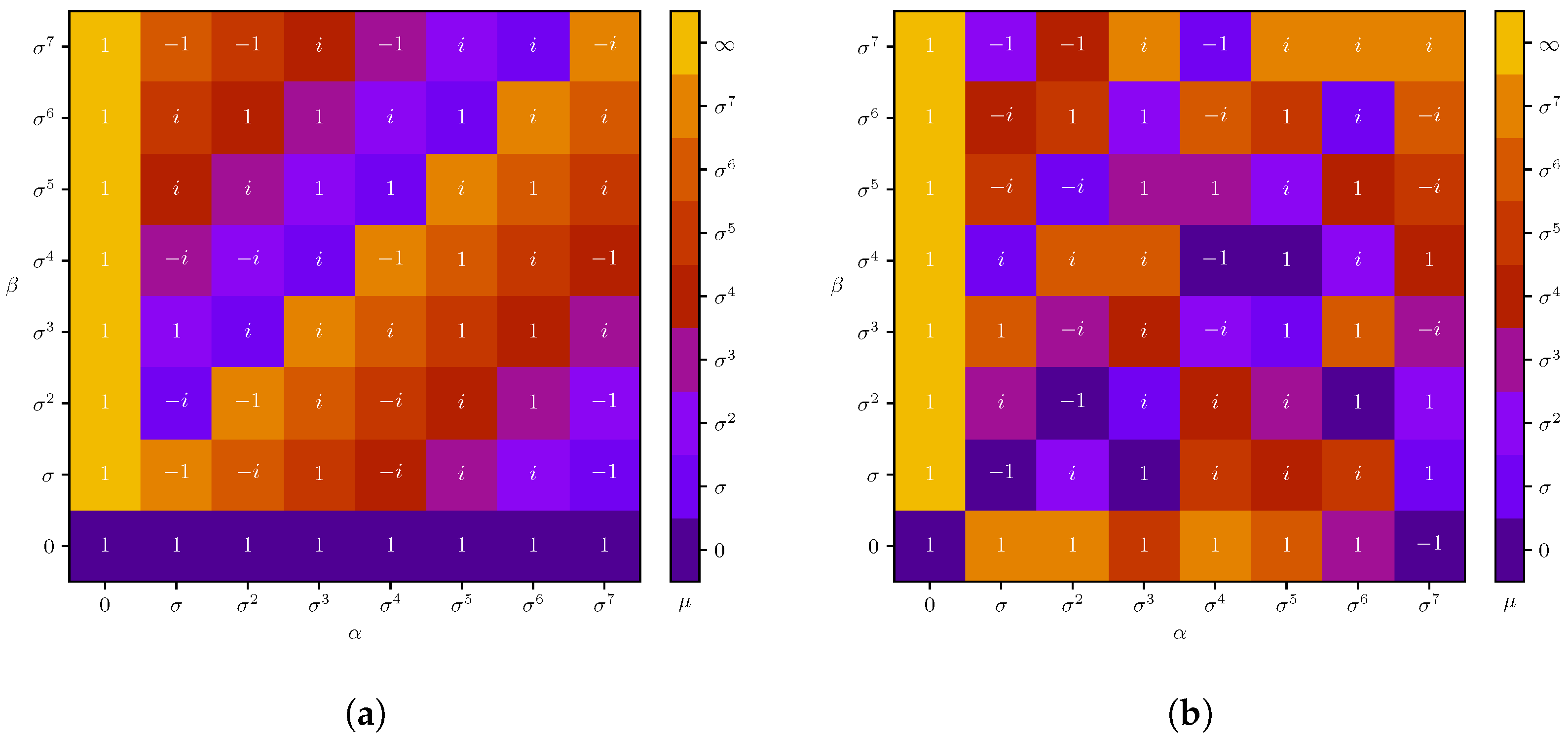
where the index labels the stabilizers/projectors (12) within this partition. Geometrically, Equations (28) and (29) represent a summation along the curves that pass through the origin, i.e., of the form (16). In other words, each point of the DPS is assigned a specific phase according to the unit commutative curve that passes through that point and corresponding to the displacement operator . In Figure 1, we plot all of the unit commutative curves and the distribution of the corresponding phases along each curve in the case of three qubits for two different partitions.
By shifting through the action of the displacement operators (23) to an arbitrary point , one obtains
where the sum is performed over all the curves passing through the point .
4. Tomographic Universality of the Discrete Wigner Function
4.1. Tomographic Property for a Given DPS Partition
The Wigner function of any stabilizer state within a partition used for the construction of is a convolution of characters computed at the points of the unit commutative curve , which labels the elements of a stabilizer with the eigenvalues , and fixes a particular stabilizer state according to (12),
as it immediately follows from spectral decomposition (17) and Equation (25).
On the other hand, it immediately follows from decomposition (30) and the unbiasement condition (13) that
which is just a delta function along the curve associated with the state :
Equation (33) represents a flip side of the tomographic condition,
In other words, the sum of the Wigner function of a state along a curve corresponding to a stabilizer state gives the probability of detecting the state in .
The properties (33) and (34) are automatically satisfied for the stabilizer states of the partition employed for the construction of the Wigner map. However, for stabilizer states from different partitions, Equations (33) and (34) do not necessarily hold. We will analyze the validity of these tomographic relations for both odd and even local dimensions.
4.2. Odd Local Dimensions
In the case of odd local dimensions, the kernel at the origin, Equation (28), takes on a simple form because the equation for phase (10):
has an explicit solution for every stabilizer of any partition:
where and due to (16). The primary property of phase (35) is its factorization, as follows from (5). As a consequence, the kernel and thus are factorized in an almost self-dual basis for any partition:
where
This implies that the mapping kernel does not depend on the particular partition of the DPS in the case of odd local dimensions. Such a statement may not be immediately obvious from the representation (29). This is because different partitions involve stabilizer states with different factorization properties (14) [28].
As a result, the tomographic conditions (33) and (34) are satisfied for any stabilizer state belonging to an arbitrary phase space partition , even if they are unrelated to the one employed for the construction of the Wigner map, i.e.,
where is a Wigner kernel corresponding to some other partition . Actually, the factorization of kernel (36) implies that the Wigner function of an arbitrary n-qudit state has exactly the same form for any DPS partition in the case of odd local dimensions.
4.3. Even Local Dimensions
The situation is significantly different for even local dimensions, . In this case, none of the solutions of Equation (10) for the phase of the displacement operators for stabilizers labelled by points of commutative curves (16), and for , admit a factorized form. A solution of the recurrence (10),
under the condition,
is fixed by choosing signs of the phases corresponding to the elements of the self-dual basis , ,
where . For instance, for all positive signs, we have [43]:
where . The non-factorized form of the phase implies that the map essentially depends on the choice of a complete set of disjoint stabilizers. In other words, it depends on the partition of the DPS into sets of commutative curves .
In general, the Wigner function of a stabilizer state from an arrangement in the (core) partition has the form (see Appendix A):
where , are the phases along , and are the phases assigned to each point of the DPS according to the partition . Therefore, Equation (40) can be reduced to the form (33) if the phases and are the same along the curve . Such curves will be referred as to Abelian curves. Obviously, all the curves that constitute a given partition are Abelian. However, there are Abelian curves outside of this partition, leading to a DWF of the corresponding stabilizer states that are delta functions:
where is a curve associated with the state in the partition . It is worth noting that these Abelian curves may possess a factorization structure (14) not present in the original partition.
The density matrix of a stabilizer state corresponding to an Abelian curve not belonging to the core partition acquires a simple form:
In other word, it is an equally weighted sum of the Wigner kernels in the core partition along the curve associated with the state . However, the reconstruction expression (18) for a stabilizer state associated with an Abelian curve does not have the form of a convex sum of the core MUB projectors.
In general, searching for Abelian curves that do not belong to a given partition typically requires an involved analytical or numerical procedure. In addition, there is the same freedom (38) in the election of the phases of the displacement operators along such curves from a partition to those of the core partition . In what follows, we give examples of Abelian curves in the case of three qubit systems.
Let us choose a partition of the DPS for the field corresponding to rays (15), and fix the phases of the stabilizers according to (39) in the same way for all slopes . We do this by choosing the all positive solutions of the recurrence relation (37) for the basis elements, i.e., , where it is always true that . This results in the following distribution of phases (where is the field generator):
The partition corresponding to the rays has the factorization structure , which means that there are three completely factorized bases and six completely non-factorized bases. In the three-qubit case, other admissible partitions include and [36,37]. Apart from the rays, there are two types of commutative curves constituting these partitions, specifically regular curves of the following form [26] (see also Appendix A):
These are characterized by non-degenerate values along the or axes and exceptional curves which are degenerated in both directions. These curves can be represented either in a parametric form or as relations of the type:
where and do not take all values of the field, but instead run only through an admissible set of points restricted by relations and , where are some fixed elements of .
We have found that for the primitive polynomial and the self-dual basis , the regular curves (44) are Abelian under the positive sign selection (38) if the following relations between parameters and are fulfilled:
- 1.
- If , then ;
- 2.
- If , then ;
- 3.
- If , there are no values producing Abelian curves, as can be observed in the example in Figure 1b, where the only Abelian curve is the ray .
For instance, the bi-factorized curves in the partition defined in Appendix B,
are Abelian, and the corresponding DWFs are
where and are eigenstates of the stabilizers
respectively. Interestingly, both exceptional curves belonging to this partition are also Abelian.
On the other hand, the curves from the same partition ,
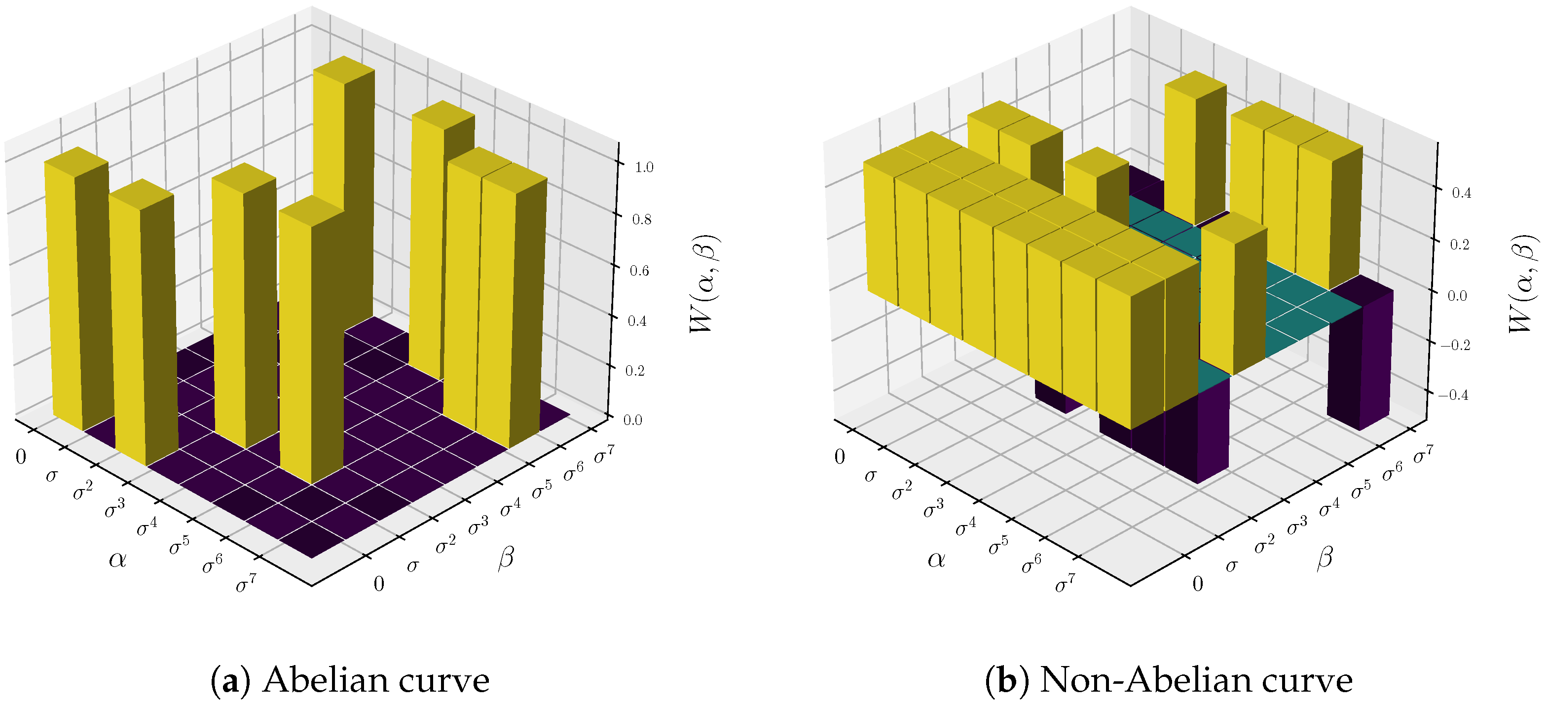
are not Abelian; thus, the DFWs corresponding to the stabilizer states are not delta functions. In Figure 2, we plot the Wigner function for the unit stabilizer states corresponding to curves (46) and (50), respectively. Reconstruction of the stabilizer states and associated with curves (46) and (50) in the form of an expansion of the ray-related (15) MUB projectors fixed by the phases in (43) (and in terms of the corresponding probabilities (18)) is given in Appendix C. As it is expected, the obtained representations (A11) and (A14) are not convex sums of the projectors (A17) and (A18).
The above-mentioned curves become Abelian for a different assignment of signs to the phases (38). For instance, curve (50) is Abelian by choosing for any . Under this assignment, the following regular curves (44) are Abelian:
- 1.
- If , then ;
- 2.
- If , then ;
- 3.
- If , .
Additionally, curve (49) is Abelian under an assignment where the signs of depend of the value of the slope .
In general, in the three-qubit case and the specific DPS partition, certain choices of phase signs can make all possible commutative curves Abelian. The inverse statement is however not true: for a given curve, it is not always possible to establish a choice of signs of so that this curve becomes Abelian for fixed phases .
5. Conclusions
The Wigner mapping kernel can be constructed as a sum of projectors onto elements of a complete set of MUBs, which are eigenstates of disjoint stabilizers corresponding to a given partition of the discrete phase space into non-intersecting commutative curves. Different partitions lead to different factorization properties of MUBs, which are required for the mapping. For qudit systems with odd local dimensions, the Wigner kernel is factorized in the same form for all possible partitions. This results in tomographic universality, reflected in the delta function form of Wigner functions of any stabilizer state corresponding to any partition.
However, in the case of n-qubit systems, the mapping kernel is not factorizable, and its form depends on the chosen discrete phase space partition [28] and on the selected set of stabilizer states in this core partition, particularly on their phases. Consequently, the qubit discrete Wigner function is not tomographically universal for an arbitrary election of phases of the stabilizer states used for Wigner map construction. Nonetheless, this property is not completely lost. It is shown that for a given partition of the DPS, there are stabilizer states corresponding to commutative curves which do not participate in the construction of the mapping kernel, such that their DWFs are delta functions. This means that the probability of detecting these states by measuring in an arbitrary state is obtained by summing the DWF along the corresponding curve. This property is directly related to the feasibility of the classical simulation of Pauli observable measurements in such n-qubit states (see Theorem 2 in [18]). However, since the measurement procedure is codified in the partition of the DPS, only some specific stabilizer states, beyond those used in the measurement scheme, are classically simulable in a given experimental setup (for a fixed DPS partition). In other words, different experimental configurations may lead to different classical simulability outcomes for stabilizer states. This highlights the role of experimental design and setup in determining the classical or quantum nature of measurement outcomes. On the other hand, it is always possible to adjust a detection scheme so that the Pauli measurements in any particular stabilizer state can be described by a non-contextual hidden variable model. This supports a previously discussed finding [18,30] that the stabilizer states cannot be considered as a resource for quantum computation [13].
Although we have only analyzed a three-qubit system, the present approach is extendable to a higher number of qubits. In particular, one can expect that for any given partition, there are sign assignments such that the DWF of an arbitrary stabilizer state acquires a delta function form; i.e., it confirms the tomographic universality of n-qubit DWFs under the freedom of the phase choice. This conjecture has been verified by extensive numerical simulations and it can be justified by the same functional form of the recurrence Equation (37) for the phase (10) of any Abelian curve.
Author Contributions
Conceptualization, I.S. and A.B.K.; Software, E.C. and A.G.; Validation, A.B.K.; Formal analysis, I.S., E.C., A.G. and A.B.K.; Investigation, I.S., E.C. and A.G.; Data curation, E.C. and A.G.; Writing—original draft, A.B.K.; Writing—review and editing, I.S., E.C. and A.B.K.; Supervision, A.B.K. All authors have read and agreed to the published version of the manuscript.
Funding
This research received no external funding.
Data Availability Statement
Data are contained within the article.
Conflicts of Interest
The authors declare no conflicts of interest.
Appendix A
In this Appendix, we derive Equation (40) in the main text. Taking into account the expansion inverse of (17):
and representation (25) of the Wigner kernel, one obtains
where the sum over denotes a sum over the points of the curve . The displacement operators and from the partitions and , respectively, according to (8), (10) carry the corresponding phases and that guarantee the Abelian property (9). Thus, one gets
which after performing a sum over and , is reduced to Equation (40).
Appendix B
In this Appendix, we recall some basic properties of commutative curves in even local dimensions. Commuting sets constituted by different monomials (stabilizers) are labelled by points of a discrete grid belonging to a non-singular curve (i.e., with no self-intersection) that passes through the origin and satisfies
A general parametric form of such a curve is given by
where the coefficients and are such that , which implies
It is worth noting that n appropriately chosen points of the curve, e.g., , are enough to generate the entire curve. This is because the set of points of these curves forms an Abelian group where each element is of order two, and therefore the group is isomorphic to .
The regular curves, which are non-degenerate in at least one of the directions or (i.e., they take on all the values of the field in such a direction), can be represented in the explicit form [26]:
where the coefficients satisfy the following commutativity restrictions:
where denotes the integer part. In particular, for even n values, the coefficients satisfy the additional restriction:
The degenerate (or exceptional) curves are characterized by multiple appearances of the admissible points in both directions and . In other words, for every point of such a curve, and take on only and different values, respectively, where and are the degrees of degenerations along the corresponding axes. The admissible points of such curves are fixed by the relations and , where are some given elements of .
The partitions of the DPS constituted by commutative curves are classified by their factorization structures (14), , where , which indicates the number and the lengths of the commuting sub-blocks of the stabilizers labelled by the points of a curve. Locally equivalent stabilizers can be labelled by points of different curves, but have the same factorization structure. On the other hand, curves with different factorization structures are not locally equivalent.
In particular, in the partition given by Equation (15), there are three completely factorized rays (, and ), i.e., of the structure , and the other six rays have the structure , so that the whole partition is .
The partitions include only curves with the factorization and always contain exceptional curves. One example of these partitions is given by the following seven regular and two exceptional curves:
- (a)
- Regular curves
- (b)
- Exceptional curves
Appendix C
In this Appendix, we provide the explicit expressions for the reconstruction of the states and associated with the curves (46) and (50) in terms of ray-related MUB projectors with the corresponding probabilities (18):
and
where the MUBs associated with the partition of the DPS in rays (15) have the form:
and the phases are defined in (43).
References
- Wigner, E. On the quantum correction for thermodynamic equilibrium. Phys. Rev. A 1932, 40, 749–759. [Google Scholar] [CrossRef]
- Bloch, F. Zur Theorie des Austauschproblems und der Remanenzerscheinung der Ferromagnetika. Z. für Phys. 1932, 74, 295–335. [Google Scholar] [CrossRef]
- Groenewold, H.J. On the principles of elementary quantum mechanics. Physica 1949, 12, 405–460. [Google Scholar] [CrossRef]
- Moyal, J.E. Quantum mechanics as a statistical theory. Math. Proc. Camb. Philos. Soc. 1947, 45, 99–124. [Google Scholar] [CrossRef]
- Mandel, L.; Wolf, E. Coherence Properties of Optical Fields. Rev. Mod. Phys. 1965, 37, 231–287. [Google Scholar] [CrossRef]
- Barker, J.R.; Murray, S. A quasi-classical formulation of the Wigner function approach to quantum ballistic transport. Phys. Lett. A 1983, 93, 271–274. [Google Scholar] [CrossRef]
- Lin, J.; Chiu, L.C. Quantum theory of electron transport in the Wigner formalism. J. Appl. Phys. 1985, 57, 1373–1376. [Google Scholar] [CrossRef]
- Berry, M.V. Semi-classical mechanics in phase space: A study of Wigner’s function. Philos. Trans. R. Soc. A 1977, 287, 237–271. [Google Scholar] [CrossRef]
- O’Connell, R.F.; Wigner, E.P. Manifestations of Bose and Fermi statistics on the quantum distribution functionfor systems of spin-0 and spin-1/2 particles. Phys. Rev. A 1984, 30, 2613–2618. [Google Scholar] [CrossRef]
- Cohen, M.; Scully, M.O. Joint Wigner distribution for spin-1/2 particles. Foud. Phys. 1986, 16, 295–310. [Google Scholar] [CrossRef]
- Wootters, W.K. A Wigner-function formulation of finite-state quantum mechanics. Ann. Phys. 1987, 176, 1–21. [Google Scholar] [CrossRef]
- Gibbons, K.S.; Hoffman, M.J.; Wootters, W.K. Discrete phase space based on finite fields. Phys. Rev. A 2004, 70, 062101. [Google Scholar] [CrossRef]
- Gottesman, D. The Heisenberg representation of quantum computers. In Group 22: International Colloquium on Group Theoretical Methods in Physics, Proceedings of 22nd International Colloquium, Group22, ICGTMP’98, Hobart, Australia, 13–17 July 1998; Corney, S.P., Delbourgo, R., Jarvis, P.D., Eds.; International Press: Cambridge, MA, USA, 1999; pp. 32–43. [Google Scholar]
- Galvão, E.F. Discrete Wigner functions and quantum computational speedup. Phys. Rev. A 2005, 71, 042302. [Google Scholar] [CrossRef]
- Cormick, C.; Galvão, E.F.; Gottesman, D.; Paz, J.P.; Pittenger, A.O. Classicality in discrete Wigner functions. Phys. Rev. A 2006, 73, 012301. [Google Scholar] [CrossRef]
- Gross, D. Hudson’s theorem for finite-dimensional quantum systems. J. Math. Phys. A 2006, 47, 122107. [Google Scholar] [CrossRef]
- Veitch, V.C.; Ferrie, C.; Gross, D.; Emerson, J. Negative quasi-probability as a resource for quantum computation. New J. Phys. 2012, 14, 113011. [Google Scholar] [CrossRef]
- Raussendorf, R.; Browne, D.E.; Delfosse, N.; Okay, C.; Bermejo-Vega, J. Contextuality and Wigner-function negativity in qubit quantum computation. Phys. Rev. A 2017, 95. [Google Scholar] [CrossRef]
- Schmid, D.; Du, H.; Shelby, J.H.; Pusey, M.F. Uniqueness of Noncontextual Models for Stabilizer Subtheories. Phys. Rev. Lett. 2022, 129, 120403. [Google Scholar] [CrossRef]
- Raussendorf, R.; Okay, C.; Zurel, M.; Feldmann, P. The role of cohomology in quantum computation with magic states. Quantum 2023, 7, 979. [Google Scholar] [CrossRef]
- Saniga, M.; Planat, M.; Rosu, H. Mutually unbiased bases and finite projective planes. J. Opt. B Quantum Semiclass. Opt. 2004, 6, L19–L20. [Google Scholar] [CrossRef]
- Ivanovic, I.D. Geometrical description of quantal state determination. J. Phys. A 1984, 14, 3241–3245. [Google Scholar] [CrossRef]
- Wootters, W.K.; Fields, B.D. Optimal State-Determination by Mutually Unbiased Measurements. Ann. Phys. 1989, 191, 363–381. [Google Scholar] [CrossRef]
- Klappenecker, A.; Rötteler, M. Constructions of mutually unbiased bases. In Lecture Notes in Computer Science Vol. 2948: Finite Fields and Applications, Procceedings of 7th International Conference, Fq7, Toulouse, France, 5–9 May 2003; Mullen, G., Poli, A., Stichtenoth, H., Eds.; Springer: Berlin/Heidelberg, Germany, 2003; pp. 137–144. [Google Scholar]
- Bandyopadhyay, S.; Boykin, P.O.; Roychowdhury, V.; Vatan, F. A new proof for the existence of mutually unbiased bases. Algorithmica 2002, 34, 512–528. [Google Scholar] [CrossRef]
- Klimov, A.B.; Romero, J.L.; Björk, G.; Sánchez-Soto, L.L. Discrete phase-space structure of n-qubit mutually unbiased bases. Ann. Phys. 2009, 324, 53–72. [Google Scholar] [CrossRef]
- Klimov, A.B.; Romero, J.L.; Björk, G.; Sánchez-Soto, L.L. Geometrical approach to mutually unbiased bases. J. Phys. A Math. Gen. 2007, 40, 9177. [Google Scholar] [CrossRef]
- Pittenger, A.O.; Rubin, M.H. Wigner functions and separability for finite systems. J. Phys. A Math. Gen. 2005, 38, 6005–6036. [Google Scholar] [CrossRef]
- Delfosse, N.; Guerin, P.A.; Bian, J.; Raussendorf, R. Wigner Function Negativity and Contextuality in Quantum Computation on Rebits. Phys. Rev. X 2015, 5, 021003. [Google Scholar] [CrossRef]
- Howard, M.; Wallman, J.; Vietch, V.; Emerson, J. Contextuality supplies the ‘magic’ for quantum computation. Nature 2014, 510, 351–355. [Google Scholar] [CrossRef] [PubMed]
- Delfosse, N.; Okay, C.; Bermejo-Vega, J.; Browne, D.E.; Raussendorf, R. Equivalence between contextuality and negativity of the Wigner function for qudits. New J. Phys. 2017, 19, 123024. [Google Scholar] [CrossRef]
- Muñoz, C.; Klimov, A.B.; Sanchez-Soto, L.L. Discrete phase-space structures and Wigner functions for N qubits. Quantum Inf. Process. 2017, 16, 158. [Google Scholar] [CrossRef]
- Lidl, R.; Niederreiter, H. Introduction to Finite Fields and Their Applications, 2nd ed.; Cambridge University Press: Cambridge, UK, 1994; ISBN 978-052-146-094-1. [Google Scholar]
- Schwinger, J. Unitary Operator Bases. Proc. Natl. Acad. Sci. USA 1960, 46, 570–579. [Google Scholar] [CrossRef] [PubMed]
- Schwinger, J. Unitary Transformations and the Action Principle. Proc. Natl. Acad. Sci. USA 1960, 46, 883–897. [Google Scholar] [CrossRef]
- Lawrence, J.; Brukner, Č.; Zeilinger, A. Mutually unbiased binary observable sets on N qubits. Phys. Rev. A 2002, 65, 032320. [Google Scholar] [CrossRef]
- Romero, J.L.; Björk, G.; Klimov, A.B.; Sánchez-Soto, L.L. Structure of the sets of mutually unbiased bases for N qubits. Phys. Rev. A 2005, 72, 062310. [Google Scholar] [CrossRef]
- Durt, T. About Weyl and Wigner tomography in finite-dimensional Hilbert spaces. Open Sys. Inf. Dyn. 2006, 13, 403–413. [Google Scholar] [CrossRef]
- Vourdas, A. Quantum systems with finite Hilbert space. Rep. Prog. Phys. 2004, 67, 267. [Google Scholar] [CrossRef]
- Vourdas, A. Factorization in finite quantum systems. J. Phys. A Math. Gen. 2003, 36, 5645. [Google Scholar] [CrossRef]
- Paz, J.P.; Roncaglia, A.J.; Saraceno, M. Qubits in phase space: Wigner-function approach to quantum-error correction and the mean-king problem. Phys. Rev. A 2005, 72, 012309. [Google Scholar] [CrossRef]
- Bjork, G.; Klimov, A.B.; Sanchez-Soto, L.L. The discrete Wigner function. In Progress in Optics, 1st ed.; Wolf, E., Ed.; Elsevier: Amsterdam, The Netherlands, 2008; Volume 51, pp. 469–516. [Google Scholar] [CrossRef]
- Klimov, A.B.; Muñoz, C.; Romero, J.L. Geometrical approach to the discrete Wigner function in prime power dimensions. J. Phys. A Math. Gen. 2006, 39, 14471. [Google Scholar] [CrossRef]
Figure 1.
Unit commutative curves along with the distribution of the respective phases (8) satisfying condition (10) for the partitions: (a), described by the rays , , ; (b) described by the curves , .

Figure 2.
The Wigner function for the unit stabilizer states corresponding to (a) the Abelian curve (46) and (b) the non-Abelian curve (50) for the partition of the DPS according to Equations (15) and (43). Note that the first Wigner function has a delta function form (48) corresponding to the Abelian curve, while the second function corresponding to a non-Abelian curve takes on negative values.

Disclaimer/Publisher’s Note: The statements, opinions and data contained in all publications are solely those of the individual author(s) and contributor(s) and not of MDPI and/or the editor(s). MDPI and/or the editor(s) disclaim responsibility for any injury to people or property resulting from any ideas, methods, instructions or products referred to in the content. |
© 2024 by the authors. Licensee MDPI, Basel, Switzerland. This article is an open access article distributed under the terms and conditions of the Creative Commons Attribution (CC BY) license (https://creativecommons.org/licenses/by/4.0/).
Share and Cite
MDPI and ACS Style
Sainz, I.; Camacho, E.; García, A.; Klimov, A.B. Tomographic Universality of the Discrete Wigner Function. Quantum Rep. 2024, 6, 58-73. https://0-doi-org.brum.beds.ac.uk/10.3390/quantum6010005
AMA Style
Sainz I, Camacho E, García A, Klimov AB. Tomographic Universality of the Discrete Wigner Function. Quantum Reports. 2024; 6(1):58-73. https://0-doi-org.brum.beds.ac.uk/10.3390/quantum6010005
Chicago/Turabian StyleSainz, Isabel, Ernesto Camacho, Andrés García, and Andrei B. Klimov. 2024. "Tomographic Universality of the Discrete Wigner Function" Quantum Reports 6, no. 1: 58-73. https://0-doi-org.brum.beds.ac.uk/10.3390/quantum6010005