Geometric Aspects of Mixed Quantum States Inside the Bloch Sphere

Abstract

When studying the geometry of quantum states, it is acknowledged that mixed states can be distinguished by infinitely many metrics. Unfortunately, this freedom causes metric-dependent interpretations of physically significant geometric quantities such as the complexity and volume of quantum states. In this paper, we present an insightful discussion on the differences between the Bures and the Sjöqvist metrics inside a Bloch sphere. First, we begin with a formal comparative analysis between the two metrics by critically discussing three alternative interpretations for each metric. Second, we explicitly illustrate the distinct behaviors of the geodesic paths on each one of the two metric manifolds. Third, we compare the finite distances between an initial state and the final mixed state when calculated with the two metrics. Interestingly, in analogy with what happens when studying the topological aspects of real Euclidean spaces equipped with distinct metric functions (for instance, the usual Euclidean metric and the taxicab metric), we observe that the relative ranking based on the concept of a finite distance between mixed quantum states is not preserved when comparing distances determined with the Bures and the Sjöqvist metrics. Finally, we conclude with a brief discussion on the consequences of this violation of a metric-based relative ranking on the concept of the complexity and volume of mixed quantum states.

1. Introduction

It is established that there exist infinitely many distinguishability metrics for mixed quantum states [1]. For this reason, there is a certain degree of arbitrariness in selecting a metric when characterizing the physical aspects of quantum states in mixed states. In particular, this freedom can cause metric-dependent explanations of geometric quantities with a clear physical significance, including the complexity [2,3,4,5,6,7,8,9,10] and volume [11,12,13,14,15,16,17,18,19,20,21,22] of quantum states. Two examples of metrics for mixed quantum states are the Bures [23,24,25,26] and the Sjöqvist [27] metrics. In ref. [28], we proposed the first explicit characterization of the Bures and Sjöqvist metrics over the manifolds of thermal states for specific spin qubit and superconducting flux qubit Hamiltonian models. We observed that while both metrics become the Fubini–Study metric in the asymptotic limiting case of the inverse temperature approaching infinity for both Hamiltonian models, the two metrics are generally distinct when far from the zero-temperature limit. The two metrics differ in the presence of nonclassical behavior specified by the noncommutativity of neighboring mixed quantum states. Such a noncommutativity, in turn, is taken into account by the two metrics differently. As a follow up of our work in [28], we used the concept of decompositions of density operators by means of ensembles of pure quantum states to present an unabridged mathematical investigation on the relation between the Sjöqvist metric and the Bures metric for arbitrary nondegenerate mixed quantum states in ref. [29]. Furthermore, to deepen our comprehension of the difference between these two metrics from a physics standpoint, we compared the general expressions of these two metrics for arbitrary thermal quantum states for quantum systems in equilibrium with a reservoir at non-zero temperature. Then, for clarity, we studied the difference between these two metrics in the case of a spin-qubit in an arbitrarily oriented uniform and stationary external magnetic field in thermal equilibrium with a finite-temperature bath. Finally, we showed in ref. [29] that the Sjöqvist metric does not satisfy the so-called monotonicity property [1], unlike the Bures metric. An interesting observable consequence in terms of the complexity behavior of this freedom in choosing between the Bures and Sjöqvist metrics was reported in ref. [2]. There, devoting our attention to geodesic lengths and curvature properties for manifolds of mixed quantum states, we recorded a softening of the information geometric complexity [30,31] on the Bures manifold compared to the Sjöqvist manifold.

In this paper, motivated by our findings in refs. [2,28,29], we present a more in-depth conceptual discussion of the differences between the Bures and the Sjöqvist metrics inside a Bloch sphere. To achieve this goal, we first begin by presenting a formal comparative analysis between the two metrics in Section 2. This analysis is based upon a critical discussion of three different alternative interpretations for each one of the two metrics. We then continue in Section 3 with an explicit illustration of the different behavior of the geodesic paths on each one of the two metric manifolds. In the same section, we also compare the finite distances between an initial and final mixed state when calculated by means of the two metrics. Inspired by what happens when studying the topological aspects of real Euclidean spaces equipped with distinct metric functions (for instance, the usual Euclidean metric and the taxicab metric), we observe in Section 4 that the relative ranking based on the concept of finite distance among mixed quantum states is not preserved when comparing distances determined with the Bures and the Sjöqvist metrics. We then discuss in Section 4 the consequences of this violation of a metric-based relative ranking on the concept of complexity and volume of mixed quantum states, along with other geometric peculiarities of the Bures and the Sjöqvist metrics inside a Bloch sphere. Our concluding remarks appear in Section 5. Finally, for the ease of presentation, some more technical details are given in Appendix A and Appendix B.

Before transitioning to our next section, we acknowledge that the presentation of the content of this paper is more suitable for specialists interested in the geometric aspects of mixed quantum states. However, for interested readers who are not so familiar with the topic, we suggest ref. [1] for a general introduction to the geometry of quantum states. Furthermore, for a tutorial on the geometry of Bures and Sjöqvist manifolds of mixed states, we refer to ref. [28]. Finally, for a partial list of more technical applications of the Bures and Sjöqvist metrics in quantum information science, we suggest refs. [32,33,34,35,36,37,38,39,40,41,42,43,44,45].

2. Line Elements

In this section, we begin with a presentation of a formal comparative analysis between the Bures and the Sjöqvist metrics inside a Bloch sphere. For completeness, we first mention in

Table 1. Examples of metrics in the space of quantum states characterized in terms of the Riemannian property and monotonicity.

Metric	Riemannian Property	Monotonicity
Bures	Yes	Yes
Hilbert–Schmidt	Yes	No
Sjöqvist	Yes	No
Trace	No	Yes

some examples of metrics for mixed quantum states and characterize them in terms of their Riemannian and monotonicity properties. For more details on the notion of monotonicity and the Riemannian property for quantum metrics, we refer to ref. [1]. Returning to our main analysis, we focus here on the geometry of single-qubit mixed quantum states characterized by density operators on a two-dimensional Hilbert space. In this case, an arbitrary density operator $\rho$ can be written as a decomposition of four linear operators (i.e., four $(2\times 2)$-matrices) given by the identity operator I and the usual Pauli vector operator $\overrightarrow{\sigma }\stackrel{\mathrm{def}}{=}\left({\sigma }_x,{\sigma }_y,{\sigma }_z\right)$ [46]. Explicitly, we have

$$\rho \stackrel{\mathrm{def}}{=}\frac{1}{2}\left(\mathrm{I}+\overrightarrow{p}·\overrightarrow{\sigma }\right),$$

(1)

where $\overrightarrow{p}\stackrel{\mathrm{def}}{=}p\widehat{p}$ denotes the three-dimensional Bloch vector. Note that p is the length $∥\overrightarrow{p}∥\stackrel{\mathrm{def}}{=}\sqrt{\overrightarrow{p}·\overrightarrow{p}}$ of the polarization vector $\overrightarrow{p}$, while $\widehat{p}$ is the unit vector. Following the vectors and one-form notation along with the line of reasoning presented in refs. [47,48,49], we can formally recast $\overrightarrow{p}$ and $\overrightarrow{\sigma }$ in Equation (1) as

$$\overrightarrow{p}\stackrel{\mathrm{def}}{=}\sum _{i=1}^3{p}^i{\widehat{e}}_i,\mathrm{and}\overrightarrow{\sigma }\stackrel{\mathrm{def}}{=}\sum _{i=1}^3{\sigma }^i{\widehat{e}}_i,$$

(2)

respectively. Observe that ${\left\{{\widehat{e}}_i\right\}}_{1\le i\le 3}$ is a set of orthonormal three-dimensional vectors satisfying ${\widehat{e}}_i·{\widehat{e}}_j={\delta }_{ij}$, with ${\delta }_{ij}$ being the Kronecker delta symbol. Moreover, we have $\left({\sigma }^1,{\sigma }^2,{\sigma }^3\right)\stackrel{\mathrm{def}}{=}\left({\sigma }_x,{\sigma }_y,{\sigma }_z\right)$. For pure states, $\rho ={\rho }^2$, tr$\left(\rho \right)=\mathrm{tr}\left({\rho }^2\right)=1$, and $p=1$. Therefore, pure states are located on the surface of the unit two-sphere. For mixed states, instead, $\rho \ne {\rho }^2$, tr$\left(\rho \right)=1$, and tr$\left({\rho }^2\right)\le 1$. Since tr$\left({\rho }^2\right)=p^2$, we have $p\le 1$. Therefore, mixed quantum states are located inside the unit two-sphere; i.e., they belong to the interior of the Bloch sphere.

In next two subsections, we study the geometric aspects of the interior of the Bloch sphere specified by the Bures and the Sjöqvist line elements.

2.1. The Bures Line Element

In the case of the Bures geometry, the infinitesimal line element $d{s}_{\mathrm{Bures}}^2\left(\overrightarrow{p},\overrightarrow{p}+d\overrightarrow{p}\right)$ between two neighboring mixed states $\rho$ and $\rho +d\rho$ corresponding to Bloch vectors $\overrightarrow{p}$ and $\overrightarrow{p}+d\overrightarrow{p}$ is given by [25,47,48]

$$d{s}_{\mathrm{Bures}}^2\left(\overrightarrow{p},\overrightarrow{p}+d\overrightarrow{p}\right)=\frac{1}{4}\left[\frac{{\left(\overrightarrow{p}·d\overrightarrow{p}\right)}^2}{1-p^2}+d\overrightarrow{p}·d\overrightarrow{p}\right]=\frac{1}{4}\left[\frac{d{p}^2}{1-p^2}+p^2(d\widehat{p}·d\widehat{p})\right].$$

(3)

The equality between the first and second expressions of $d{s}_{\mathrm{Bures}}^2\left(\overrightarrow{p},\overrightarrow{p}+d\overrightarrow{p}\right)$ in Equation (3) can be checked by first noting that $\widehat{p}·\widehat{p}=1$ implies $\widehat{p}·d\widehat{p}=0$. This, in turn, yields the relations $d\overrightarrow{p}·d\overrightarrow{p}=d{p}^2+p^{2}d\widehat{p}·d\widehat{p}$ and ${\left(\overrightarrow{p}·d\overrightarrow{p}\right)}^2=p^{2}d{p}^2$. Finally, the use of these two identities allows us to arrive at the equality between the two expressions in Equation (3).

In what follows, we propose three interpretations for the Bures metric which originate from a critical reconsideration of the original work by Braunstein and Caves in refs. [47,48].

2.1.1. First Interpretation

We wish to critically discuss the structure of $d{s}_{\mathrm{Bures}}^2\left(\overrightarrow{p},\overrightarrow{p}+d\overrightarrow{p}\right)$ in Equation (3). To interpret the term $d\widehat{p}·d\widehat{p}$ in $d{s}_{\mathrm{Bures}}^2\left(\overrightarrow{p},\overrightarrow{p}+d\overrightarrow{p}\right)$, it is convenient to recast the polarization vector in spherical coordinates as $\overrightarrow{p}=\left(p^1,p^2,p^3\right)\stackrel{\mathrm{def}}{=}\left(psin\left(\theta \right)cos\left(\phi \right),psin\left(\theta \right)sin\left(\phi \right),pcos\left(\theta \right)\right)$. Note that in spherical coordinates, we also have $\left({\widehat{e}}_1,{\widehat{e}}_2,{\widehat{e}}_3\right)=\left({\widehat{e}}_r,{\widehat{e}}_{\theta },{\widehat{e}}_{\phi }\right)$. It then follows that $d\overrightarrow{p}·d\overrightarrow{p}=d{p}^2+p^2\left(d{\theta }^2+{sin}^2\left(\theta \right)d{\phi }^2\right)$ and ${\left(\overrightarrow{p}·d\overrightarrow{p}\right)}^2=p^{2}d{p}^2$. Finally, noting that the unit polarization vector is $\widehat{p}=\left(sin\left(\theta \right)cos\left(\phi \right),sin\left(\theta \right)sin\left(\phi \right),cos\left(\theta \right)\right)$, we get after some algebra that $d\widehat{p}·d\widehat{p}=d{\theta }^2+{sin}^2\left(\theta \right)d{\phi }^2$. From this last relation, it clearly follows that $d\widehat{p}·d\widehat{p}$ represents the usual line element $d{\Omega }^2\stackrel{\mathrm{def}}{=}$$d{\theta }^2+{sin}^2\left(\theta \right)d{\phi }^2$ on a unit two-sphere. Therefore, when using spherical coordinates, the line element in Equation (3) can be recast as

$$d{s}_{\mathrm{Bures}}^2\left(\overrightarrow{p},\overrightarrow{p}+d\overrightarrow{p}\right)=\frac{1}{4}\left[\frac{d{p}^2}{1-p^2}+p^2(d{\theta }^2+{sin}^2\left(\theta \right)d{\phi }^2)\right].$$

(4)

From Equation (3), it happens that when p is kept constant and equal to $p_0$, a surface specified by the relation $p=p_0$ inside the Bloch sphere exhibits the geometry of a two-sphere of area $4\pi p_0^2$. As mentioned in refs. [47,48], the term $d{p}^2/\left(1-p^2\right)$ in $d{s}_{\mathrm{Bures}}^2\left(\overrightarrow{p},\overrightarrow{p}+d\overrightarrow{p}\right)$ implies that the inside of the Bloch sphere is not flat, but curved. Indeed, moving away from the origin of the sphere, the circumference $C\left(p\right)\stackrel{\mathrm{def}}{=}2\pi p$ of a circle of radius p on the two-sphere grows as $dC/ds\sim p^{\prime }\stackrel{\mathrm{def}}{=}dp/ds$, with s being the affine parameter. The distance $l\left(p\right)\stackrel{\mathrm{def}}{=}{\int }_{s\left(0\right)}^{s\left(p\right)}$$p^{\prime }/{\left(1-p^2\right)}^{1/2}ds$ from the center, instead, grows as $dl/ds\sim$$p^{\prime }/{\left(1-p^2\right)}^{1/2}\ge p^{\prime }$. Therefore, $l\left(p\right)$ grows at a faster rate than $C\left(p\right)$. This discrimination in growth rates for $C\left(p\right)$ and $l\left(p\right)$ signifies that the interior of the Bloch sphere is curved.

2.1.2. Second Interpretation

A second useful coordinate system to further gain insights into the Bures line element in Equation (3) is specified by considering a change in variables defined by $p\stackrel{\mathrm{def}}{=}sin\left(\chi \right)$, with $\chi$ being the hyperspherical angle with $0\le \chi \le \pi /2$. In this set of coordinates, $4d{s}_{\mathrm{Bures}}^2\left(\overrightarrow{p},\overrightarrow{p}+d\overrightarrow{p}\right)$ reduces to

$$4d{s}_{\mathrm{Bures}}^2=d{\chi }^2+{sin}^2\left(\chi \right)d\widehat{p}·d\widehat{p},$$

(5)

with $d\widehat{p}·d\widehat{p}=d{\Omega }^2\stackrel{\mathrm{def}}{=}$$d{\theta }^2+{sin}^2\left(\theta \right)d{\phi }^2$. Note that Equation (5) for the Bures metric is exactly the (intrinsic) metric on the unit three-sphere $S^3$, where $\chi$, $\theta$, and $\phi$ are the angular coordinates on the sphere. For completeness, we remark that the metric for the $(N+1)$-sphere can be written in terms of the metric for the N-sphere, with the introduction of a new hyperspherical angle [1]. Two additional considerations are in order here. First, the four-dimensional vector $x^{\mu }\left(s\right)\equiv \left(x^0\left(s\right),\overrightarrow{x}\left(s\right)\right)$ with $0\le \mu \le 3$, such that $d{x}^{\mu }d{x}_{\mu }=4d{s}_{\mathrm{Bures}}^2=d{\chi }^2+{sin}^2\left(\chi \right)d\widehat{p}·d\widehat{p}$, can be written as $x^{\mu }\left(s\right)=x^0\left(s\right){\widehat{e}}_0\left(s\right)+\overrightarrow{x}\left(s\right)$. The quantity $x^0\left(s\right)\stackrel{\mathrm{def}}{=}\chi \left(s\right)$ is the component of $x^{\mu }\left(s\right)$ along the direction ${\widehat{e}}_0\left(s\right)\stackrel{\mathrm{def}}{=}\overrightarrow{\chi }/\chi$, with ${\widehat{e}}_0\left(s\right)·{\widehat{e}}_i\left(s\right)=0$ for any $1\le i\le 3$. The three-dimensional vector $\overrightarrow{x}\left(s\right)$ given by

$$\overrightarrow{x}\left(s\right)=\int sin\left[\chi \left(s\right)\right]\frac{d\widehat{p}\left(s\right)}{ds}ds,$$

(6)

specifies the remaining three coordinates of $x^{\mu }\left(s\right)$ along the directions ${\widehat{e}}_1\left(s\right)\stackrel{\mathrm{def}}{=}{e}_r\left(s\right)$, ${\widehat{e}}_2\left(s\right)\stackrel{\mathrm{def}}{=}{e}_{\theta }\left(s\right)$, and ${\widehat{e}}_3\left(s\right)\stackrel{\mathrm{def}}{=}{e}_{\phi }\left(s\right)$. From Equation (6), we point out the presence of a correlational structure between the motion along ${\widehat{e}}_0\left(s\right)$ and the “spatial” directions ${\widehat{e}}_i\left(s\right)$ with $1\le i\le 3$. This correlational structure is a manifestation of the fact that for the Bures geometry, radial and angular motions inside the Bloch sphere are correlated, since the dynamical geodesic equations are specified by a set of second-order coupled nonlinear differential equations when using a set of spherical coordinates [2]. Second, remembering that the line element in the usual cylindrical coordinates $\left(\rho ,\phi ,z\right)$ is $d{s}_{\mathrm{cylinder}}^2=d{z}^2+d{\Omega }_{\mathrm{cylinder}}^2$, where $d{\Omega }_{\mathrm{cylinder}}^2\stackrel{\mathrm{def}}{=}d{\rho }^2+{\rho }^{2}d{\phi }^2$, we observe that the structure of the Bures line element rewritten as in Equation (5) is suggestive of the structure of a line element in the standard cylindrical coordinates once we make the connection between the pair $\left(\chi ,d\Omega \right)$ and the pair $\left(\rho ,d{\Omega }_{\mathrm{cylinder}}\right)$. Then, one can link a cylinder with a variable radius in the case of the Bures geometry. In particular, it is worth mentioning at this point that the non-constant radius in the Bures case is upper bounded by the constant value that defines the radius in the Sjöqvist geometry (as we shall see in the next subsection). These geometric insights emerging from this simple change in coordinates would lead one to reasonably expect different lengths of the geodesic paths in the two geometries studied here. This will be discussed in more detail in the next section, however.

2.1.3. Third Interpretation

An alternative third set of coordinates for the Bures line element in Equation (3) is given by the four coordinates $x^{\mu }$ with $0\le \mu \le 3$ given by $x^{\mu }=\left(x^0,\overrightarrow{x}\right)\stackrel{\mathrm{def}}{=}\left(\sqrt{1-p^2},\overrightarrow{p}\right)$ with $\overrightarrow{p}=p\widehat{p}$. Indeed, from $x^0=\sqrt{1-p^2}$, we get ${\left(d{x}^0\right)}^2={\left(\overrightarrow{p}·d\overrightarrow{p}\right)}^2/(1-p^2)$. Therefore, when employing this coordinate system, the inside of the Bloch sphere can be described by a three-dimensional surface defined by the constraint relation ${\left(x^0\right)}^2+\overrightarrow{x}·\overrightarrow{x}=1$. Moreover, the geometry of the surface is induced by the four-dimensional flat Euclidean line element [25],

$$4d{s}_{\mathrm{Bures}}^2={\left(d{x}^0\right)}^2+d\overrightarrow{x}·d\overrightarrow{x}.$$

(7)

Note that Equation (7) for the Bures metric is the (extrinsic) metric on the unit three-sphere $S^3$ viewed as embedded in ${\mathbb{R}}^4$. The geodesic paths emerging from $d{s}_{\mathrm{Bures}}^2$ in Equation (7) are great circles on the three-sphere. In terms of the arc length s, these geodesics can be recast as [47,48]

$$x^{\mu }\left(s\right)=u^{\mu }cos\left(s\right)+v^{\mu }sin\left(s\right),$$

(8)

where $u^{\mu }=\left(u^0,\overrightarrow{u}\right)\stackrel{\mathrm{def}}{=}\left(cos\left(\chi \right),\widehat{n}sin\left(\chi \right)\right)$, $v^{\mu }=\left(v^0,\overrightarrow{v}\right)\stackrel{\mathrm{def}}{=}\left(sin\left(\xi \right),\widehat{m}cos\left(\xi \right)\right)$, $\widehat{n}·\widehat{n}=\widehat{m}·\widehat{m}=1$, and $-\left(\widehat{n}·\widehat{m}\right)tan\left(\chi \right)=tan\left(\xi \right)$. This last relation assures that $u^{\mu }\perp v^{\mu }$, so that Equation (7) is satisfied for $x^{\mu }\left(s\right)$ given in Equation (8).

We are now ready to critically discuss the Sjöqvist line element by mimicking the discussion performed for the Bures line element.

2.2. The Sjöqvist Line Element

In the case of the Sjöqvist geometry, the infinitesimal line element $d{s}_{\mathrm{Sjöqvist}}^2\left(\overrightarrow{p},\overrightarrow{p}+d\overrightarrow{p}\right)$ between two neighboring mixed states $\rho$ and $\rho +d\rho$ corresponding to Bloch vectors $\overrightarrow{p}$ and $\overrightarrow{p}+d\overrightarrow{p}$ is given by [27]

$$d{s}_{\mathrm{Sjöqvist}}^2\left(\overrightarrow{p},\overrightarrow{p}+d\overrightarrow{p}\right)=\frac{1}{4}\left[\frac{2p^2-1}{p^4\left(1-p^2\right)}{\left(\overrightarrow{p}·d\overrightarrow{p}\right)}^2+\frac{d\overrightarrow{p}·d\overrightarrow{p}}{p^2}\right]=\frac{1}{4}\left[\frac{d{p}^2}{1-p^2}+(d\widehat{p}·d\widehat{p})\right].$$

(9)

The equality between the first and second expressions of $d{s}_{\mathrm{Sjöqvist}}^2\left(\overrightarrow{p},\overrightarrow{p}+d\overrightarrow{p}\right)$ in Equation (9) can be verified by first observing that $\widehat{p}·\widehat{p}=1$ implies $\widehat{p}·d\widehat{p}=0$. This, in turn, leads to the relations $d\overrightarrow{p}·d\overrightarrow{p}=d{p}^2+p^{2}d\widehat{p}·d\widehat{p}$ and ${\left(\overrightarrow{p}·d\overrightarrow{p}\right)}^2=p^{2}d{p}^2$. Finally, exploiting these two relations, we arrive at the equality between the two expressions in Equation (9).

We remark that Sjöqvist in ref. [27] was the first to seek a deeper understanding of the physics behind the metric, with the concept of mixed state geometric phases playing a key role. However, for completeness, we also point out that what we call the “Sjöqvist interferometric metric” first appeared as a special case of a more general family of metrics proposed in a more formal mathematical setting in refs. [50,51] by Andersson and Heydari. In this generalized setting, different metrics arise from different gauge theories, they are specified by distinct notions of horizontality, and, finally, they can be well defined for both nondegenerate and degenerate mixed quantum states. A great part of the underlying gauge theory of this generalized family of metrics was developed in ref. [52]. A suitable comprehensive reference to read about such a generalized family of metrics is Chapter 5 in Andersson’s thesis [53], where, in particular, the singular properties of Sjöqvist metrics are discussed in Section 5.3.2. For further technical details on this matter, we refer to ref. [53] and the references therein.

2.2.1. First Interpretation

We begin by noting that the term $d{p}^2/\left(1-p^2\right)$ in $d{s}_{\mathrm{Sjöqvist}}^2\left(\overrightarrow{p},\overrightarrow{p}+d\overrightarrow{p}\right)$ implies that the inside of the Bloch sphere is not flat, but curved. In particular, the interpretation of this term follows exactly the discussion provided in the previous subsection for the Bures case. Moreover, similarly to the Bures case, the term $d\widehat{p}·d\widehat{p}$ remains the standard line element $d{\Omega }^2\stackrel{\mathrm{def}}{=}$$d{\theta }^2+{sin}^2\left(\theta \right)d{\phi }^2$ on a unit two-sphere. Therefore, when using spherical coordinates, the line element in Equation (9) can be recast as

$$d{s}_{\mathrm{Sjöqvist}}^2\left(\overrightarrow{p},\overrightarrow{p}+d\overrightarrow{p}\right)=\frac{1}{4}\left[\frac{d{p}^2}{1-p^2}+d{\theta }^2+{sin}^2\left(\theta \right)d{\phi }^2\right].$$

(10)

Unlike what happens in the Bures case, when p is kept constant and equal to $p_0$, a surface specified by the relation $p=p_0$ inside the Bloch sphere exhibits the geometry of a two-sphere of area $4\pi$ in the Sjöqvist case. The area $4\pi$ of this two-sphere is greater than the area $4\pi p_0^2$ that specifies the Bures case and, in addition, does not depend on the choice of the constant value $p_0$ of p. This is a signature of the fact that, in the Sjöqvist case, the accessible regions inside the Bloch sphere have volumes greater than those specifying the Bures geometry. Indeed, this observation was first pointed out in ref. [2] and shall be further discussed in the forthcoming interpretations.

2.2.2. Second Interpretation

In analogy to the second interpretation proposed for the Bures metric, a convenient coordinate system to further gain insights into the Sjöqvist line element in Equation (9) can be changing the variables defined by $p\stackrel{\mathrm{def}}{=}sin\left(\chi \right)$, with $\chi$ being the hyperspherical angle with $0\le \chi \le \pi /2$. In this set of coordinates, $4d{s}_{\mathrm{Sjöqvist}}^2\left(\overrightarrow{p},\overrightarrow{p}+d\overrightarrow{p}\right)$ reduces to

$$4d{s}_{\mathrm{Sjöqvist}}^2\left(\overrightarrow{p},\overrightarrow{p}+d\overrightarrow{p}\right)=d{\chi }^2+d\widehat{p}·d\widehat{p},$$

(11)

with $d\widehat{p}·d\widehat{p}=d{\Omega }^2\stackrel{\mathrm{def}}{=}$$d{\theta }^2+{sin}^2\left(\theta \right)d{\phi }^2$. Observe that Equation (11) for the Sjöqvist metric exhibits a structure that is similar to that of the metric on $S^1\times S^2$, the Cartesian product of the unit one-sphere $S^1$ with the unit two-sphere $S^2$. This Cartesian product is responsible for the uncorrelated structure between the hyperspherical angle coordinate and the pair of angular coordinates $\left(\theta ,\phi \right)$ (i.e., the polar and azimuthal angles, respectively). This uncorrelated structure, in turn, manifests itself with an expression of the metric on $S^1\times S^2$, which is simply the sum of the metrics on $S^1$ and $S^2$. More specifically, comparing Equations (5) and (11), we note that in the Sjöqvist case, unlike the Bures case, the “temporal” and “spatial” spatial components of the metric are no longer correlated. In particular, the analogue of $\overrightarrow{x}\left(s\right)$ in Equation (6) reduces to

$$\overrightarrow{x}\left(s\right)=\int \frac{d\widehat{p}\left(s\right)}{ds}ds.$$

(12)

From Equation (12) we emphasize the absence of a correlational structure between the motion along ${\widehat{e}}_0\left(s\right)$ and the “spatial” directions ${\widehat{e}}_i\left(s\right)$ with $1\le i\le 3$. Interestingly, the lack of this correlational structure manifests itself when using spherical coordinates to describe the Sjöqvist geometry. Specifically, it emerges from the fact that the radial and angular motions inside the Bloch sphere are not correlated since the dynamical geodesic equations are specified by a set of second-order uncoupled nonlinear differential equations [2]. Lastly, recalling that the line element in the usual cylindrical coordinates $\left(\rho ,\phi ,z\right)$ is $d{s}_{\mathrm{cylinder}}^2=d{z}^2+d{\Omega }_{\mathrm{cylinder}}^2$, where $d{\Omega }_{\mathrm{cylinder}}^2\stackrel{\mathrm{def}}{=}d{\rho }^2+{\rho }^{2}d{\phi }^2$, we note that the structure of the Sjöqvist line element recast as in Equation (11) is reminiscent of the structure of a line element in the traditional cylindrical coordinates once we connect the pair $\left(\chi ,d\Omega \right)$ and the pair $\left(\rho ,d{\Omega }_{\mathrm{cylinder}}\right)$. Then, unlike what happens in the Bures case, one can associate a cylinder with a constant value of its radius in the case of the Sjöqvist geometry. In particular, the constant value of the radius upper bounds any value that the varying radius can assume in the Bures case. Again, as previously mentioned, these geometric insights that arise from this simple change in coordinates would lead one to expect different lengths of geodesic paths in the two geometries studied here. However, this will be studied in more detail in the next section. In what follows, instead, we present our third and last interpretation.

2.2.3. Third Interpretation

Following the third interpretation presented for the Bures case, we adapt the four coordinates $x^{\mu }$ with $0\le \mu \le 3$ given by $x^{\mu }=\left(x^0,\overrightarrow{x}\right)\stackrel{\mathrm{def}}{=}\left(\sqrt{1-p^2},\overrightarrow{p}\right)$ with $\overrightarrow{p}=p\widehat{p}$ to the Sjöqvist line element $d{s}_{\mathrm{Sjöqvist}}^2\left(\overrightarrow{p},\overrightarrow{p}+d\overrightarrow{p}\right)$ in Equation (9). After some algebra, we get

$$4d{s}_{\mathrm{Sjöqvist}}^2={\omega }_{x^0}\left(p\right){\left(d{x}^0\right)}^2+{\omega }_{\overrightarrow{x}}\left(p\right)d\overrightarrow{x}·d\overrightarrow{x},$$

(13)

with ${\omega }_{x^0}\left(p\right)\stackrel{\mathrm{def}}{=}\left(2p^2-1\right)/p^4$ and ${\omega }_{\overrightarrow{x}}\left(p\right)\stackrel{\mathrm{def}}{=}1/p^2$. Note that Equation (13) for the Sjöqvist metric is the (extrinsic) metric for $S^1\times S^2$ embedded in ${\mathbb{R}}^4$. The embedding of $S^1\times S^2$ in ${\mathbb{R}}^4$ appears to be more complicated than that of $S^3$ in ${\mathbb{R}}^4$. This complication, in turn, leads to behavior of the Sjöqvist metric which is more irregular than that observed in the Bures case. More specifically, comparing Equations (7) and (13), we note that unlike what happens in the Bures case, the inside of the Bloch sphere is no longer a unit three-sphere embedded in a four-dimensional flat Euclidean space with geodesics given by great circles on it when using the four coordinates $x^{\mu }$. In particular, the metric $4d{s}_{\mathrm{Sjöqvist}}^2$ as expressed in Equation (13) is not regular since its signature is not constant. Indeed, ${\omega }_{x^0}\left(p\right)\ge 0$ for $p\ge 1/\sqrt{2}$ and ${\omega }_{x^0}\left(p\right)\le 0$ for $0\le p\le 1/\sqrt{2}$. An essential singularity appears at $p=0$ (i.e., for maximally mixed states). This observation, although obtained from a different perspective, is in agreement with what was originally noticed in ref. [27]. Finally, the geodesic paths change as well. Indeed, the geodesics ${\left[x^{\mu }\left(s\right)\right]}_{\mathrm{Bures}}\stackrel{\mathrm{def}}{=}\left[x^0\left(s\right),\overrightarrow{x}\left(s\right)\right]$ in Equation (7) are formally replaced by ${\left[x^{\mu }\left(s\right)\right]}_{\mathrm{Sjöqvist}}$ expressed in terms of ${\left[x^0\left(s\right)\right]}_{\mathrm{Sjöqvist}}$ and ${\left[\overrightarrow{x}\left(s\right)\right]}_{\mathrm{Sjöqvist}}$ as

$${\left[x^0\left(s\right)\right]}_{\mathrm{Bures}}\to {\left[x^0\left(s\right)\right]}_{\mathrm{Sjöqvist}}\stackrel{\mathrm{def}}{=}\int \sqrt{\left|{\omega }_{x^0}\left(p\right)\right|}\frac{d{x}^0\left(s\right)}{ds}ds,$$

(14)

and

$${\left[\overrightarrow{x}\left(s\right)\right]}_{\mathrm{Bures}}\to {\left[\overrightarrow{x}\left(s\right)\right]}_{\mathrm{Sjöqvist}}\stackrel{\mathrm{def}}{=}\int \frac{1}{\sqrt{{\omega }_{\overrightarrow{x}}\left(p\right)}}\frac{d\overrightarrow{x}\left(s\right)}{ds}ds,$$

(15)

respectively. For completeness and following the terminology of the previous subsection, we point out that $p\left(s\right)$ in Equations (14) and (15) equals $p\left(s\right)\stackrel{\mathrm{def}}{=}{\left\{1-{\left[cos\left(\chi \right)cos\left(s\right)+sin\left(\xi \right)sin\left(s\right)\right]}^2\right\}}^{1/2}$ such that $0\le p\left(s\right)\le 1$.

In this section, we focused our attention on grasping physical insights from the infinitesimal line elements for the Bures and the Sjöqvist metrics inside a Bloch sphere in Equations (3) and (9), respectively. In the next section, we shall further explore some of our insights by extending our focus to the difference between the finite distances of geodesic paths connecting mixed quantum states on these two metric manifolds.

3. Finite Distances

In this section, we turn our attention to the study of the behaviors of the geodesic paths on each one of the two metric manifolds, i.e., Bures and Sjöqvist manifolds. Furthermore, we also offer a comparison between the finite distances between arbitrary initial and final mixed states when calculated by means of the above-mentioned metrics. For clarity, we remark that to compare finite distances between mixed quantum states in the Bloch ball calculated with the Bures and Sjöqvist metrics, it is sufficient to focus on points in the $xz$-plane. This is a consequence of two facts. First, distances are preserved under rotations. Second, it is possible to construct a suitable composition of two $\mathrm{SO}(3$; $\mathbb{R})$ rotations acting on arbitrary Bloch vectors for mixed states, say ${\overrightarrow{p}}_1$ and ${\overrightarrow{p}}_2$, such that the distances $\mathcal{L}\left({\overrightarrow{p}}_1,{\overrightarrow{p}}_2\right)=\mathcal{L}\left({\overrightarrow{p}}_{1,new},{\overrightarrow{p}}_{2,new}\right)$ with ${\overrightarrow{p}}_{1,new}$ and ${\overrightarrow{p}}_{2,new}$ belong to the $xz$-plane. For further details, we refer to Appendix A.

3.1. The Bures Distance

We begin by using spherical coordinates $\left(r,\theta ,\phi \right)$ and keep $\phi =$ const. Then, geodesics are obtained by minimizing ∫$d{s}_{\mathrm{Bures}}$ over all curves connecting points $\left(r_a,{\theta }_a\right)$ and $\left(r_b,{\theta }_b\right)$. More specifically, one arrives at the curve $\left[{\theta }_a,{\theta }_b\right]\ni \theta \mapsto r_{\mathrm{Bures}}\left(\theta \right)\in \left[0,1\right]$ that minimizes the length ${\mathcal{L}}_{\mathrm{Bures}}(\overrightarrow{a}$, $\overrightarrow{b})$ defined as

$${\mathcal{L}}_{\mathrm{Bures}}(\overrightarrow{a},\overrightarrow{b})\stackrel{\mathrm{def}}{=}{\int }_{s_a}^{s_b}\sqrt{d{s}_{\mathrm{Bures}}^2}=\frac{1}{2}{\int }_{{\theta }_a}^{{\theta }_b}\mathrm{L}\left(r^{\prime },r,\theta \right)d\theta ,$$

(16)

with $d{s}_{\mathrm{Bures}}^2$ in Equation (4). In Equation (16), $r^{\prime }\stackrel{\mathrm{def}}{=}dr/d\theta$ and $\mathrm{L}\left(r^{\prime },r,\theta \right)$ is the Lagrangian-like function defined as

$$\mathrm{L}\left(r^{\prime },r,\theta \right)\stackrel{\mathrm{def}}{=}\sqrt{r^2+\frac{r^{\prime 2}}{1-r^2}}.$$

(17)

From Equation (36), note that $\mathrm{L}=\mathrm{L}\left(r^{\prime },r\right)$ in Equation (17) does not explicitly depend on $\theta$. Therefore, $\partial \mathrm{L}/\partial \theta =0$. In this case, it happens that the Euler–Lagrange equation

$$\frac{d}{d\theta }\frac{\partial \mathrm{L}\left(r^{\prime },r\right)}{\partial r^{\prime }}-\frac{\partial \mathrm{L}\left(r^{\prime },r\right)}{\partial r}=0,$$

(18)

reduces to the well-known Beltrami identity in Lagrangian mechanics,

$$\mathrm{L}\left(r^{\prime },r\right)-r^{\prime }\frac{\partial \mathrm{L}\left(r^{\prime },r\right)}{\partial r^{\prime }}=\mathrm{const}.$$

(19)

Indeed, making use of Equation (18) together with the identity

$$\frac{d\mathrm{L}\left(r^{\prime },r\right)}{d\theta }=\frac{\partial \mathrm{L}\left(r^{\prime },r\right)}{\partial r^{\prime }}{r}^{\prime \prime }+\frac{\partial \mathrm{L}\left(r^{\prime },r\right)}{\partial r}{r}^{\prime },$$

(20)

we get

$$\frac{d\mathrm{L}\left(r^{\prime },r\right)}{d\theta }=\frac{d}{d\theta }\left(r^{\prime }\frac{\partial \mathrm{L}\left(r^{\prime },r\right)}{\partial r^{\prime }}\right).$$

(21)

Finally, Equation (21) leads to the so-called Beltrami identity in Equation (19). Using Equations (17) and (19), we obtain

$$\frac{r^2}{\sqrt{r^2+\frac{r^{\prime 2}}{1-r^2}}}=\mathrm{const}.\equiv {\mathrm{c}}_{\mathrm{B}}.$$

(22)

Manipulating Equation (22) and imposing the boundary conditions $r\left({\theta }_a\right)=r_a$ and $r\left({\theta }_b\right)=r_b$, we obtain

$${\int }_{r_a}^{r_b}\frac{dr}{\sqrt{r^2\left(\frac{r^2}{{\mathrm{c}}_{\mathrm{B}}^2}-1\right)\left(1-r^2\right)}}={\int }_{{\theta }_a}^{{\theta }_b}d\theta ,$$

(23)

with $0<{\mathrm{c}}_{\mathrm{B}}\le r\le 1$. For notational simplicity, let us set ${\mathrm{a}}_{\mathrm{B}}^2\stackrel{\mathrm{def}}{=}1/{\mathrm{c}}_{\mathrm{B}}^2>1$. Then, integration of Equation (23) by use of Mathematica yields

$$\mathrm{I}\left(r\right)\stackrel{\mathrm{def}}{=}\int \frac{dr}{\sqrt{r^2\left(\frac{r^2}{{\mathrm{c}}_{\mathrm{B}}^2}-1\right)\left(1-r^2\right)}}=\frac{r\sqrt{r^2-1}\sqrt{{\mathrm{a}}_{\mathrm{B}}^2{r}^2-1}}{\sqrt{-r^2\left(r^2-1\right)\left({\mathrm{a}}_{\mathrm{B}}^2{r}^2-1\right)}}{tanh}^{-1}\left(\frac{\sqrt{r^2-1}}{\sqrt{{\mathrm{a}}_{\mathrm{B}}^2{r}^2-1}}\right)+\mathrm{const}.$$

(24)

Manipulating Equation (24), $\mathrm{I}\left(r\right)$ in Equation (24) becomes

$$\mathrm{I}\left(r\right)=-arctan\left(\frac{\sqrt{1-r^2}}{\sqrt{{\mathrm{a}}_{\mathrm{B}}^2{r}^2-1}}\right)+\mathrm{const}.$$

(25)

Finally, substituting Equation (25) into Equation (23), the radial geodesic path in the Bures case can be recast as [2]

$$r_{\mathrm{Bures}}\left(\theta \right)=\sqrt{\frac{1+{tan}^2\left[{\mathcal{A}}_{\mathrm{B}}\left(r_a,r_a^{\prime }\right)-\left(\theta -{\theta }_a\right)\right]}{1+{\mathrm{a}}_{\mathrm{B}}^2\left(r_a,r_a^{\prime }\right){tan}^2\left[{\mathcal{A}}_{\mathrm{B}}\left(r_a,r_a^{\prime }\right)-\left(\theta -{\theta }_a\right)\right]}},$$

(26)

where the constants ${\mathcal{A}}_{\mathrm{B}}\left(r_a,r_a^{\prime }\right)$ and ${\mathrm{a}}_{\mathrm{B}}^2\left(r_a,r_a^{\prime }\right)$ in Equation (26) are given by

$${\mathcal{A}}_{\mathrm{B}}\left(r_a,r_a^{\prime }\right)\stackrel{\mathrm{def}}{=}arctan\left(\sqrt{{\left(1-r_a^2\right)}^2{\left(\frac{r_a}{r_a^{\prime }}\right)}^2}\right),\mathrm{and}{\mathrm{a}}_{\mathrm{B}}^2\left(r_a,r_a^{\prime }\right)\stackrel{\mathrm{def}}{=}\frac{1}{r_a^2}+{\left(\frac{r_a^{\prime }}{r_a}\right)}^2\frac{1}{r_a^2\left(1-r_a^2\right)},$$

(27)

respectively. At this point, we recall that the Bures distance between two density operators ${\rho }_1$ and ${\rho }_2$ is given by [25],

$${\mathcal{L}}_{\mathrm{Bures}}\left({\rho }_1,{\rho }_2\right)\stackrel{\mathrm{def}}{=}\sqrt{2}{\left[1-\mathrm{tr}\left(\sqrt{\sqrt{{\rho }_1}{\rho }_2\sqrt{{\rho }_1}}\right)\right]}^{1/2}.$$

(28)

Furthermore, ${\mathcal{L}}_{\mathrm{Bures}}\left({\rho }_1,{\rho }_2\right)$ in Equation (28) can be expressed in terms of the fidelity between two density operators ${\rho }_1$ and ${\rho }_2$, defined as [54,55]

$$\mathrm{F}\left({\rho }_1,{\rho }_2\right)\stackrel{\mathrm{def}}{=}{\left(\mathrm{tr}\left(\sqrt{\sqrt{{\rho }_1}{\rho }_2\sqrt{{\rho }_1}}\right)\right)}^2.$$

(29)

Therefore, combining Equations (28) and (29), the Bures distance ${\mathcal{L}}_{\mathrm{Bures}}\left({\rho }_1,{\rho }_2\right)$ becomes

$${\mathcal{L}}_{\mathrm{Bures}}\left({\rho }_1,{\rho }_2\right)=\sqrt{2}{\left[1-\sqrt{\mathrm{F}\left({\rho }_1,{\rho }_2\right)}\right]}^{1/2}.$$

(30)

Then, focusing on qubit states, the fidelity $\mathrm{F}\left({\rho }_1,{\rho }_2\right)$ in Equation (29) reduces to [54]

$$\mathrm{F}\left({\rho }_1,{\rho }_2\right)=\mathrm{tr}\left({\rho }_1{\rho }_2\right)+2\sqrt{det\left({\rho }_1\right)det\left({\rho }_2\right)},$$

(31)

where ${\rho }_1$ and ${\rho }_2$ are given by

$${\rho }_1=\rho \left(\overrightarrow{a}\right)\stackrel{\mathrm{def}}{=}\frac{\mathrm{I}+\overrightarrow{a}·\overrightarrow{\sigma }}{2},\mathrm{and}{\rho }_2=\rho \left(\overrightarrow{b}\right)\stackrel{\mathrm{def}}{=}\frac{\mathrm{I}+\overrightarrow{b}·\overrightarrow{\sigma }}{2},$$

(32)

respectively. Using Equations (32) and (31), ${\mathcal{L}}_{\mathrm{Bures}}\left({\rho }_1,{\rho }_2\right)$ in Equation (30) reduces to

$${\mathcal{L}}_{\mathrm{Bures}}\left({\rho }_1,{\rho }_2\right)=\sqrt{2}{\left[1-\sqrt{2\left(\frac{1+\overrightarrow{a}·\overrightarrow{b}}{4}+\sqrt{\frac{1-{\overrightarrow{a}}^2}{4}\frac{1-{\overrightarrow{b}}^2}{4}}\right)}\right]}^{1/2}.$$

(33)

For Bloch vectors $\overrightarrow{a}\stackrel{\mathrm{def}}{=}{r}_a{\widehat{n}}_a$ and $\overrightarrow{b}\stackrel{\mathrm{def}}{=}{r}_b{\widehat{n}}_b$ in the $xz$-plane, we have ${\widehat{n}}_a\stackrel{\mathrm{def}}{=}\left(sin\left({\theta }_a\right),0,cos\left({\theta }_a\right)\right)$ and ${\widehat{n}}_b\stackrel{\mathrm{def}}{=}\left(sin\left({\theta }_b\right),0,cos\left({\theta }_b\right)\right)$, with ${\theta }_a$ and ${\theta }_b$ in $\left[0,\pi \right]$. Therefore, in this scenario, ${\mathcal{L}}_{\mathrm{Bures}}\left({\rho }_1,{\rho }_2\right)={\mathcal{L}}_{\mathrm{Bures}}({\rho }_1\left(\overrightarrow{a}\right),{\rho }_2\left(\overrightarrow{b}\right))={\mathcal{L}}_{\mathrm{Bures}}(\overrightarrow{a}$, $\overrightarrow{b})$ in Equation (33) is equal to

$${\mathcal{L}}_{\mathrm{Bures}}(\overrightarrow{a},\overrightarrow{b})=\sqrt{2}{\left[1-\sqrt{2\left(\frac{1+r_a{r}_{b}cos\left({\theta }_a-{\theta }_b\right)}{4}+\sqrt{\frac{1-r_a^2}{4}\frac{1-r_b^2}{4}}\right)}\right]}^{1/2}.$$

(34)

The expression of ${\mathcal{L}}_{\mathrm{Bures}}(\overrightarrow{a}$, $\overrightarrow{b})$ in Equation (34) helps us to evaluate the finite distance between arbitrary mixed states $\rho \left(\overrightarrow{a}\right)\stackrel{\mathrm{def}}{=}(\mathrm{I}+\overrightarrow{a}·\overrightarrow{\sigma })/2$ and $\rho \left(\overrightarrow{b}\right)\stackrel{\mathrm{def}}{=}(\mathrm{I}+\overrightarrow{b}·\overrightarrow{\sigma })/2$ belonging to the $xz$-plane and, thus, arbitrary states in the Bloch ball (for details, see Appendix A).

3.2. The Sjöqvist Distance

Following Sjöqvist’s work in ref. [27], we focus on finding geodesic paths that connect points (i.e., mixed quantum states) in the Bloch ball that lie in a plane that contains the origin. Employing spherical coordinates $\left(r,\theta ,\phi \right)$ and maintaining $\phi =$ const., geodesics can be obtained by minimizing ∫$d{s}_{\mathrm{Sjöqvist}}$ over all curves connecting points $\overrightarrow{a}\leftrightarrow \left(r_a,{\theta }_a\right)$ and $\overrightarrow{b}\leftrightarrow \left(r_b,{\theta }_b\right)$. More specifically, we aim to get the curve $\left[{\theta }_a,{\theta }_b\right]\ni \theta \mapsto r_{\mathrm{Sjöqvist}}\left(\theta \right)\in \left(0,1\right]$ that minimizes the length ${\mathcal{L}}_{\mathrm{Sjöqvist}}(\overrightarrow{a}$, $\overrightarrow{b})$ given by

$${\mathcal{L}}_{\mathrm{Sjöqvist}}(\overrightarrow{a},\overrightarrow{b})\stackrel{\mathrm{def}}{=}{\int }_{s_a}^{s_b}\sqrt{d{s}_{\mathrm{Sjöqvist}}^2}=\frac{1}{2}{\int }_{{\theta }_a}^{{\theta }_b}\mathrm{L}\left(r^{\prime },r,\theta \right)d\theta ,$$

(35)

with $d{s}_{\mathrm{Sjöqvist}}^2$ in Equation (10). In Equation (35), $r^{\prime }\stackrel{\mathrm{def}}{=}dr/d\theta$ and $\mathrm{L}\left(r^{\prime },r,\theta \right)$ is the Lagrangian-like function defined as

$$\mathrm{L}\left(r^{\prime },r,\theta \right)\stackrel{\mathrm{def}}{=}\sqrt{1+\frac{r^{\prime 2}}{1-r^2}}.$$

(36)

Following the similar derivation of the Euler–Lagrange equations leading to Equation (22) in the previous subsection for the Bures metric, we obtain

$$\frac{1}{\sqrt{1+\frac{r^{\prime 2}}{1-r^2}}}=\mathrm{const}.\equiv {\mathrm{c}}_{\mathrm{S}},$$

(37)

that is,

$$\frac{r^{\prime 2}}{1-r^2}=\mathrm{const}.\equiv \mathrm{k}\stackrel{\mathrm{def}}{=}\frac{1-{\mathrm{c}}_{\mathrm{S}}^2}{{\mathrm{c}}_{\mathrm{S}}^2},$$

(38)

Integrating Equation (38) and imposing the boundary conditions $r\left({\theta }_a\right)=r_a$, $r\left({\theta }_b\right)=r_b$, with ${\theta }_{\mathrm{initial}}={\theta }_a$ and ${\theta }_{\mathrm{final}}={\theta }_b$, we obtain the geodesic path

$$r_{\mathrm{Sjöqvist}}\left(\theta \right)=sin\left\{\frac{{sin}^{-1}\left(r_b\right)-{sin}^{-1}\left(r_a\right)}{{\theta }_b-{\theta }_a}\theta +\frac{{sin}^{-1}\left(r_a\right)+{sin}^{-1}\left(r_b\right)}{2}-\frac{1}{2}\frac{{\theta }_a+{\theta }_b}{{\theta }_b-{\theta }_a}\left[{sin}^{-1}\left(r_b\right)-{sin}^{-1}\left(r_a\right)\right]\right\}.$$

(39)

We remark that the expression of $r_{\mathrm{Sjöqvist}}\left(\theta \right)$ in Equation (39) can be recast, alternatively, in terms of the boundary conditions on the initial position $r\left({\theta }_a\right)=r_a$ and the initial speed $r^{\prime }\left({\theta }_a\right)=r_a^{\prime }$. We get, after some algebra [2],

$$r_{\mathrm{Sjöqvist}}\left(\theta \right)=sin\left[\frac{r_a^{\prime }}{\sqrt{1-r_a^2}}\left(\theta -{\theta }_a\right)+{sin}^{-1}\left(r_a\right)\right].$$

(40)

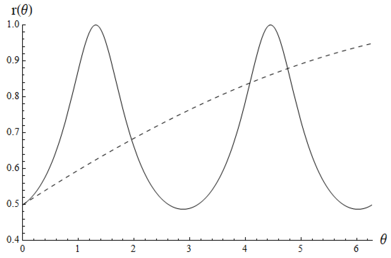
As a consistency check, we observe that we correctly recover Equation (18) in ref. [27] when we set ${\theta }_{\mathrm{initial}}=0$ in Equation (39). For illustrative purposes, we present in Figure 1a plot of the Bures and Sjöqvist curves $r_{\mathrm{Bures}}\left(\theta \right)$ in Equation (26) and $r_{\mathrm{Sjoqvist}}\left(\theta \right)$ in Equation (40), respectively, for identical boundary conditions specified by the initial position and the initial speed. Finally, after inserting $r_{\mathrm{Sjöqvist}}\left(\theta \right)$ in Equation (39) into the expression for $\mathrm{L}\left(r^{\prime },r,\theta \right)$ in Equation (36), ${\mathcal{L}}_{\mathrm{Sjöqvist}}(\overrightarrow{a}$, $\overrightarrow{b})$ in Equation (35) reduces to [27]

$${\mathcal{L}}_{\mathrm{Sjöqvist}}(\overrightarrow{a},\overrightarrow{b})=\frac{1}{2}\sqrt{{\left({\theta }_b-{\theta }_a\right)}^2+{\left[{sin}^{-1}\left(r_b\right)-{sin}^{-1}\left(r_a\right)\right]}^2}.$$

(41)

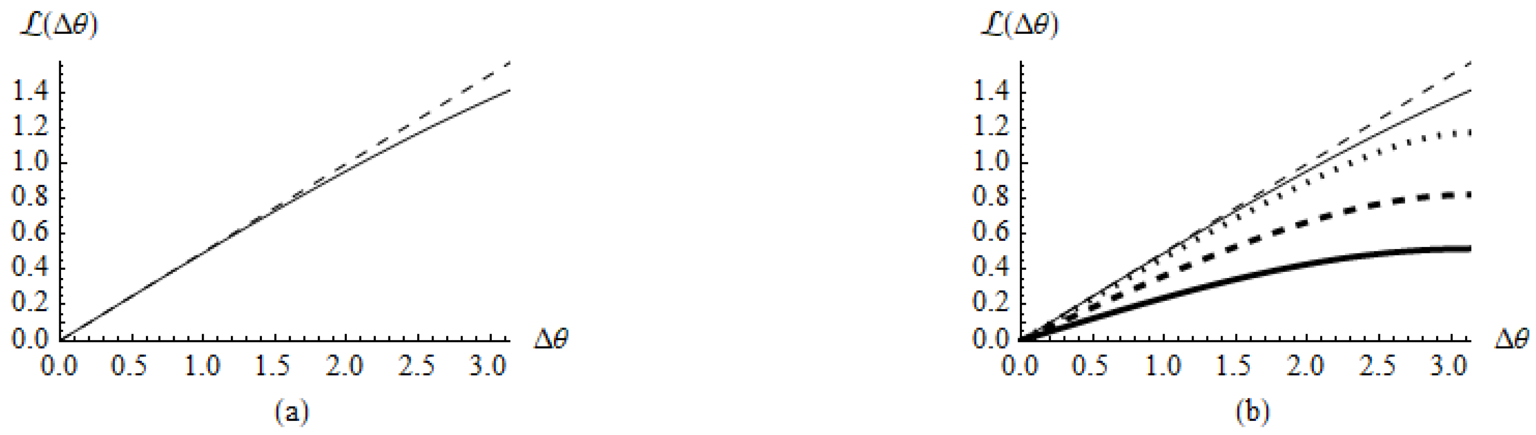
The expression of ${\mathcal{L}}_{\mathrm{Sjöqvist}}(\overrightarrow{a}$, $\overrightarrow{b})$ in Equation (41) allows us to calculate the finite distance between arbitrary mixed states $\rho \left(\overrightarrow{a}\right)\stackrel{\mathrm{def}}{=}(\mathrm{I}+\overrightarrow{a}·\overrightarrow{\sigma })/2$ and $\rho \left(\overrightarrow{b}\right)\stackrel{\mathrm{def}}{=}(\mathrm{I}+\overrightarrow{b}·\overrightarrow{\sigma })/2$ laying in the $xz$-plane and, thus, between arbitrary states in the Bloch ball (for details, see Appendix A). For illustrative purposes, we plot in part (a) of Figure 2 the Sjöqvist distance ${\mathcal{L}}_{\mathrm{Sjöqvist}}\left(\Delta \theta \right)$ in Equation (41) and the Bures distance ${\mathcal{L}}_{\mathrm{Bures}}\left(\Delta \theta \right)$ in Equation (34) versus $\Delta \theta \stackrel{\mathrm{def}}{=}{\theta }_b-{\theta }_a$, with $0\le \Delta \theta \le \pi$, with the assumption that $r_a=r_b=1$. In part (b) of Figure 2, instead, we compare the Sjöqvist and Bures distances as in (a) but for different values of $r_a=r_b=$ const. with const.$\in \left\{1,0.95,0.75,0.5\right\}$. We observe that while the Sjöqvist distance does not depend on a particular value of the const., the Bures distance depends on the specific value of the const. In any case, we have $0\le$${\mathcal{L}}_{\mathrm{Bures}}\left(\Delta \theta \right)\le {\mathcal{L}}_{\mathrm{Sjöqvist}}\left(\Delta \theta \right)\le \pi /2$. For completeness, we recall that the geodesic distance between two orthogonal pure states represented by antipodal points on the Bloch sphere is $\pi$, whereas the corresponding Fubini–Study distance is $\pi /2$. In the limit of $r_a=r_b=1$, the Bures distance in Equation (34) reduces to the Fubini–Study distance $\left|\Delta \theta \right|/2$ with $\Delta \theta \stackrel{\mathrm{def}}{=}{\theta }_b-{\theta }_a$ only approximately, since ${\mathcal{L}}_{\mathrm{Bures}}\left(\Delta \theta \right)=\left|\Delta \theta \right|/2+O\left({\left|\Delta \theta \right|}^3\right)$ when $\left|\Delta \theta \right|\ll 1$. In the same limiting case of $r_a=r_b=1$, instead, the Sjöqvist distance in Equation (41) reduces to the Fubini–Study distance $\left|\Delta \theta \right|/2$ in an exact manner.

Figure 1. Illustrative depiction of Bures and Sjöqvist curves $r_{\mathrm{Bures}}\left(\theta \right)$ (solid line) and $r_{\mathrm{Sjoqvist}}\left(\theta \right)$ (dashed line), respectively, for identical boundary conditions specified by the initial position ($r\left({\theta }_a\right)=r_a\stackrel{\mathrm{def}}{=}1/2$) and the initial speed ($r^{\prime }\left({\theta }_a\right)=r_a^{\prime }\stackrel{\mathrm{def}}{=}0.1$). Note that ${\theta }_a\le \theta \le {\theta }_b$, with ${\theta }_a\stackrel{\mathrm{def}}{=}0$ and ${\theta }_b\stackrel{\mathrm{def}}{=}2\pi$.

Figure 1. Illustrative depiction of Bures and Sjöqvist curves $r_{\mathrm{Bures}}\left(\theta \right)$ (solid line) and $r_{\mathrm{Sjoqvist}}\left(\theta \right)$ (dashed line), respectively, for identical boundary conditions specified by the initial position ($r\left({\theta }_a\right)=r_a\stackrel{\mathrm{def}}{=}1/2$) and the initial speed ($r^{\prime }\left({\theta }_a\right)=r_a^{\prime }\stackrel{\mathrm{def}}{=}0.1$). Note that ${\theta }_a\le \theta \le {\theta }_b$, with ${\theta }_a\stackrel{\mathrm{def}}{=}0$ and ${\theta }_b\stackrel{\mathrm{def}}{=}2\pi$.

Thanks to Equations (34) and (41), we are now ready to provide some intriguing discussion points in the next section.

4. Discussion

To better motivate and understand the relevance of our forthcoming discussion, we briefly summarize some of the main results we found in past investigations on a comparative analysis of the Bures and Sjoqvist metrics. In ref. [2], we found that the manifold of mixed states equipped with the Bures (Sjöqvist) metric is an isotropic (anisotropic) manifold of constant (non-constant) sectional curvature. The isotropy of the manifold, the inequality ${\mathcal{L}}_{\mathrm{Bures}}(\overrightarrow{a},\overrightarrow{b})\le$${\mathcal{L}}_{\mathrm{Sjöqvist}}(\overrightarrow{a},\overrightarrow{b})$ between the path lengths, and, in addition, the presence of a correlational structure in the equations of geodesic motion (which is absent in the Sjöqvist case) between radial and angular directions are at the root of the softening in the complexity of the geodesic evolution on Bures manifolds. Indeed, correlational structures cause the shrinkage of the explored volumes of regions on the manifold underlying the geodesic evolution. This shrinkage, finally, can be detected by means of the so-called information geometric complexity (i.e., the volume of the parametric region explored by the system during its evolution from the initial to the final configuration on the underlying manifold [31]). For a summary of the specific properties of Bures and Sjöqvist metrics in terms of sectional curvatures, path lengths, and information geometric complexities, we refer to Table III and Appendix E in ref. [2]. We also point out that we originally observed in ref. [28] that the Bures and Sjöqvist metrics characterize, in general, the departure from the classical behavior by means of the noncommutativity of neighboring mixed states in dissimilar manners. This discrepancy was first tested by studying geometric aspects of the Bures and Sjöqvist manifolds emerging from a superconducting flux Hamiltonian model in ref. [28]. Later, this discrepancy was elegantly conceptualized (see Equations (36) and (38) in ref. [29]) and, in addition, explicitly discussed for a spin-qubit in an arbitrarily oriented, uniform, and stationary magnetic field in thermal equilibrium with a finite-temperature reservoir in ref. [29].

In this section, we briefly comment on some previously unnoticed geometric features that emerge from the Bures and Sjöqvist finite distances in Equations (34) and (41) obtained in Section 3. To make our discussion closer to classical geometric and topological arguments, we carry out a comparative discussion highlighting formal similarities between the classical (Euclidean, Taxicab) metrics in the $xz$-plane of ${\mathbb{R}}^2$ and the quantum (Bures, Sjöqvist) metrics inside the Bloch sphere. Let us denote by $d_{\mathrm{Euclid}}$ and $d_{\mathrm{Taxicab}}$ the usual Euclidean and Taxicab metric functions, respectively. For completeness, we recall that $d_{\mathrm{Euclid}}(\overrightarrow{a},\overrightarrow{b})\stackrel{\mathrm{def}}{=}\sqrt{{\left(a_x-b_x\right)}^2+{\left(a_z-b_z\right)}^2}$ and $d_{\mathrm{Taxicab}}(\overrightarrow{a},\overrightarrow{b})\stackrel{\mathrm{def}}{=}\left|a_x-b_x\right|+\left|a_z-b_z\right|$ with $\overrightarrow{a}\stackrel{\mathrm{def}}{=}\left(a_x,a_z\right),\overrightarrow{b}\stackrel{\mathrm{def}}{=}\left(b_x,b_z\right)$ in ${\mathbb{R}}^2$. First, we observe that although $\left({\mathbb{R}}^2,d_{\mathrm{Euclid}}\right)$ and $\left({\mathbb{R}}^2,d_{\mathrm{Taxicab}}\right)$ are topologically equivalent metric spaces [56], we have that $d_{\mathrm{Euclid}}\left(P_i,P_{i^{\prime }}\right)\le d_{\mathrm{Euclid}}\left(P_k,P_{k^{\prime }}\right)$ does not imply that $d_{\mathrm{Taxicab}}\left(P_i,P_{i^{\prime }}\right)\le d_{\mathrm{Taxicab}}\left(P_k,P_{k^{\prime }}\right)$ with $i\ne i^{\prime }$ and $k\ne k^{\prime }$. Therefore, a relative ranking of pairs of points specified in terms of distances between the pairs themselves, with closer pairs of points ranking higher than those further away, is not preserved when using Euclidean and Taxicab metrics. For instance, consider a set ${\mathcal{S}}_1$ of three points in ${\mathbb{R}}^2$ given in Cartesian coordinates by ${\mathcal{S}}_1\stackrel{\mathrm{def}}{=}\left\{P_1\stackrel{\mathrm{def}}{=}\left(0,0\right),P_2\stackrel{\mathrm{def}}{=}\left(0,1\right),P_3\stackrel{\mathrm{def}}{=}((1+\sqrt{2})/4,(1+\sqrt{2})/4)\right\}$. One notices that $d_{\mathrm{Euclid}}\left(P_1,P_2\right)=1\ge 0.85\simeq d_{\mathrm{Euclid}}\left(P_1,P_3\right)$. However, when using the Taxicab metric, we have $d_{\mathrm{Taxicab}}\left(P_1,P_2\right)=1\le 1.21\simeq d_{\mathrm{Taxicab}}\left(P_1,P_3\right)$. Interestingly, the conservation of this type of ranking of pairs of points is violated also when comparing the Bures and Sjöqvist metrics. For instance, consider a set ${\mathcal{S}}_2$ of four points (i.e., mixed quantum states) $P_i\leftrightarrow \rho \left(P_i\right)=(\mathrm{I}+{\overrightarrow{a}}_i·\overrightarrow{\sigma })/2$ with ${\overrightarrow{a}}_i$ assumed to belong to the $xz$-plane and specified by the pair of spherical coordinates $\left(r_{a_i},{\theta }_{a_i}\right)$ given by ${\mathcal{S}}_2\stackrel{\mathrm{def}}{=}\left\{P_1\stackrel{\mathrm{def}}{=}\left(1/2,0\right),P_2\stackrel{\mathrm{def}}{=}\left(1/2,\pi \right),P_3\stackrel{\mathrm{def}}{=}(1/8,0),P_4\stackrel{\mathrm{def}}{=}(1/4,\pi )\right\}$. Then, in terms of the Bures metric, we find $d_{\mathrm{Bures}}\left(P_1,P_2\right)\simeq 0.52\ge 0.19\simeq d_{\mathrm{Bures}}\left(P_3,P_4\right)$. However, when using the Sjöqvist metric, we get $d_{\mathrm{Sjöqvist}}\left(P_1,P_2\right)=\pi /2\simeq 1.570\le 1.572\simeq d_{\mathrm{Sjöqvist}}\left(P_3,P_4\right)$. Clearly, $d_{\mathrm{Bures}}\left(P_i,P_j\right)=d_{\mathrm{Bures}}\left({\overrightarrow{a}}_i,{\overrightarrow{a}}_j\right)={\mathcal{L}}_{\mathrm{Bures}}\left({\overrightarrow{a}}_i,{\overrightarrow{a}}_j\right)$, as defined in Equation (34). Similarly, $d_{\mathrm{Sjöqvist}}\left(P_i,P_j\right)=d_{\mathrm{Sjöqvist}}\left({\overrightarrow{a}}_i,{\overrightarrow{a}}_j\right)={\mathcal{L}}_{\mathrm{Sjöqvist}}\left({\overrightarrow{a}}_i,{\overrightarrow{a}}_j\right)$, as defined in Equation (41). We also emphasize here that unlike what happens in the Bures geometry, in the Sjöqvist geometry, it is possible to identify pairs of two points, say $\left(P_i,P_{i^{\prime }}\right)$ and $\left(P_k,P_{k^{\prime }}\right)$, that seem to be visually rankable which, in actuality, are at the same distance from each other (and, thus, non-rankable according to our previously mentioned notion of relative ranking). For example, following the terminology introduced for the set ${\mathcal{S}}_2$, consider the new set of points ${\mathcal{S}}_3$ defined as ${\mathcal{S}}_3\stackrel{\mathrm{def}}{=}\left\{P_1\stackrel{\mathrm{def}}{=}\left(1/4,0\right),P_2\stackrel{\mathrm{def}}{=}\left(1/4,\pi \right),P_3\stackrel{\mathrm{def}}{=}(1/2,0),P_4\stackrel{\mathrm{def}}{=}(1/2,\pi )\right\}$. Then, when employing the Sjöqvist metric, we find $d_{\mathrm{Sjöqvist}}\left(P_1,P_2\right)=d_{\mathrm{Sjöqvist}}\left(P_3,P_4\right)=\pi /2$, even though the pair of points $\left(P_3,P_4\right)$ seems to be visually more distant than the pair of points $\left(P_1,P_2\right)$. However, when employing the Bures metric, we get $d_{\mathrm{Bures}}\left(P_1,P_2\right)\simeq 0.25\le 0.52\simeq d_{\mathrm{Bures}}\left(P_3,P_4\right)$. This latter inequality is consistent with our visual intuition associated with seeing these points as mixed states inside the Bloch sphere. Clearly, these different geometric features between Bures and Sjöqvist geometries can be ascribed to the formal structure of the expressions for the finite distances in Equations (34) and (41), respectively, that we have obtained in the previous section. Second, in addition to the fact that $d_{\mathrm{Euclid}}\left(P_i,P_j\right)\le d_{\mathrm{Taxicab}}\left(P_i,P_j\right)\leftrightarrow d_{\mathrm{Bures}}\left(P_i,P_j\right)\le d_{\mathrm{Sjöqvist}}\left(P_i,P_j\right)$ for arbitrary points $P_i$ and $P_j$, it can be noted that a given probe point in the Sjöqvist manifold appears to be locally surrounded by a greater number of points at the same distance from the source. This, in turn, can be regarded as an indicator of the presence of a higher degree of complexity during the change from an initial point (source state) to a final point (target state). Therefore, this set of points of discussion that we are offering here seems to give additional support to the apparent emergence of a softer degree of complexity in Bures manifolds when compared with Sjöqvist manifolds [2]. For clarity, we remark that the proof of the inequality $d_{\mathrm{Euclid}}\left(P_i,P_j\right)\le d_{\mathrm{Taxicab}}\left(P_i,P_j\right)$ can be found in any standard topology book, including ref. [56]. The proof of the inequality $d_{\mathrm{Bures}}\left(P_i,P_j\right)\le d_{\mathrm{Sjöqvist}}\left(P_i,P_j\right)$.

Instead, follows from the analyses presented in refs. [27,29]. In particular, its origin can be traced back to the fact that both quantum metrics originate from a specific minimization procedure that, for the Bures metric, occurs in a larger space of unitary matrices. For technical details on this minimization procedure, we refer to refs. [27,29]. For completeness, we also point out that once we find a single violation of either the former (classical) or the latter (quantum) inequalities, we can find several sets of points that would yield the same violation. From a classical geometry standpoint, this is a consequence of the fact that distances are invariant under isometries. In particular, limiting our discussion to the case at hand, any planar isometry mapping input points in ${\mathbb{R}}^2$ to output points in ${\mathbb{R}}^2$ is either a pure translation, a pure rotation about some center, or a reflection followed by a translation (i.e., a glide reflection). Moreover, the composition of two isometries is an isometry. From a quantum standpoint, instead, an isometry is an inner-product-preserving transformation that maps, in general, between Hilbert spaces with different dimensions. In the particular scenario in which input and output Hilbert spaces have the same dimensions, the isometry is simply a unitary operation. For a general discussion on the role of isometries in quantum information and computation, we refer to refs. [57,58]. Finally, for an illustrative visualization of the Euclidean, Taxicab, Bures, and Sjöqvist geometries that summarizes most of our discussion points, we refer to Figure 3. Interestingly, inspired by the expression of the Bures fidelity F${}_{\mathrm{Bures}}(\overrightarrow{a}$, $\overrightarrow{b})={\left[1-{\mathcal{L}}_{\mathrm{Bures}}^2(\overrightarrow{a},\overrightarrow{b})/{\left({\mathcal{L}}_{\mathrm{Bures}}^2\right)}_{max}\right]}^2$ with ${\left({\mathcal{L}}_{\mathrm{Bures}}\right)}_{max}=\sqrt{2}$, one may think of considering a sort of Sjöqvist fidelity given by F${}_{\mathrm{Sjöqvist}}(\overrightarrow{a}$, $\overrightarrow{b})={\left[1-{\mathcal{L}}_{\mathrm{Sjöqvist}}^2(\overrightarrow{a},\overrightarrow{b})/{\left({\mathcal{L}}_{\mathrm{Sjöqvist}}^2\right)}_{max}\right]}^2$ with ${\left({\mathcal{L}}_{\mathrm{Sjöqvist}}\right)}_{max}=\pi /2$. From these fidelities, define the ratio $\mathcal{R}(\overrightarrow{a}$, $\overrightarrow{b})\stackrel{\mathrm{def}}{=}$F${}_{\mathrm{Sjöqvist}}(\overrightarrow{a}$, $\overrightarrow{b})/$F${}_{\mathrm{Bures}}(\overrightarrow{a}$, $\overrightarrow{b})$ with $\overrightarrow{a}$, $\overrightarrow{b}$ as in Figure 3 (for example). Then, one can check that the area of the two-dimensional parametric region with parameters r and $\theta$ and specified by the conditions $0\le \mathcal{R}(\overrightarrow{a}$, $\overrightarrow{b})\le 1$, i.e., the region where Bures fidelity is larger than the Sjöqvist fidelity, is greater than $50\%$ of the total accessible two-dimensional parametric region with area given by $\pi$ (i.e., the Lebesgue measure ${\mu }_{\mathrm{Lebesgue}}\left({\left[0,1\right]}_r\times {\left[0,\pi \right]}_{\theta }\right)$ of the interval ${\left[0,1\right]}_r\times {\left[0,\pi \right]}_{\theta }$). Therefore, this type of approximate reasoning can be viewed as a semi-quantitiative indication of the higher degree of distinguishability of mixed quantum states by means of the Bures metric. Clearly, a deeper comprehension of these facts would require an analysis extended to arbitrary initial parametric configurations along with a more rigorously defined version of $\mathcal{R}(\overrightarrow{a}$, $\overrightarrow{b})$. Nevertheless, we believe that interesting insights emerge from our approximate semi-quantitative discussion proposed here. Summing up, our investigation suggests that the higher sensitivity of the length of geodesic paths connecting a given pair of initial and final mixed states of a quantum system in the Bures case is caused by the lower density of accessible final states that are equidistant from a chosen initial source state. This lower density, in turn, can be attributed to the shorter length of geodesic paths in the Bures case. Finally, the shortness of these paths is a consequence of the manner in which the quantumness (or, alternatively, non-classicality) of mixed quantum states is geometrically quantified with the Bures metric [28] (i.e., the above-mentioned way characterized by a minimization procedure in a larger space of unitary matrices [29]). We are now ready for our conclusions.

5. Conclusions

In this paper, building on our recent works in refs. [2,28,29], we presented a more comprehensive discussion on the differences between the Bures and the Sjöqvist metrics inside a Bloch sphere. First, inspired by the works of Caves and Braunstein in refs. [47,48], we offered a formal comparative analysis between the two metrics by critically discussing three alternative interpretations for each metric. For the Bures metric, the three interpretations appear in Equations (4), (5), and (7). For the Sjöqvist metric, instead, the corresponding three interpretations emerge from Equations (10), (11), and (13), respectively. Second, we illustrated (Figure 1) in an explicit fashion the different behaviors of the geodesic paths (Equations (26) and (40) for the Bures and Sjöqvist metrics cases, respectively) on each one of the two metric manifolds. Third, we compared (Figure 2) the finite distances between an initial and a final mixed state when calculated with the two metrics (Equations (34) and (41) for the Bures and Sjöqvist metrics cases, respectively). Thanks to Equations (34) and (41) for ${\mathcal{L}}_{\mathrm{Bures}}(\overrightarrow{a}$, $\overrightarrow{b})$ and ${\mathcal{L}}_{\mathrm{Sjöqvist}}(\overrightarrow{a}$, $\overrightarrow{b})$, respectively, we were able to provide some intriguing discussion points (along with a visual aid coming from Figure 3) concerning some similarities between classical (Euclidean, Taxicab) metrics in ${\mathbb{R}}^2$ and quantum (Bures, Sjöqvist) metrics inside the Bloch sphere. In particular, we argued that the fact that the Sjöqvist metric yields longer finite distances, denser clouds of states that are equidistant from a fixed source state, and, finally, an unnatural violation of the distance-based relative ranking of pairs of points inside the Bloch sphere is at the origin of the higher degree of complexity of the Sjöqvist manifold compared with the Bures manifold as reported in ref. [2].

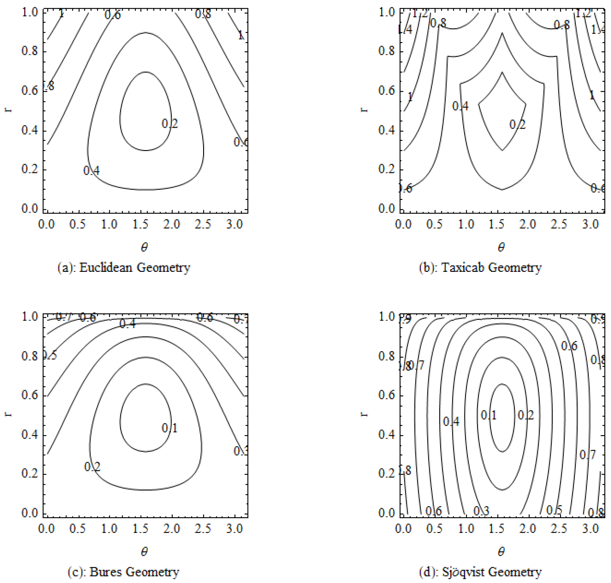
In the usual three-dimensional physical space, we ordinarily state that the reason why it is difficult to distinguish two points is because they are close together. In classical and quantum geometry, one tends to invert this line of reasoning and claim that two points on a statistical manifold must be very close together because it is hard to differentiate them [59]. In particular, within the geometry of mixed quantum states, increasing distances seem to correspond to more reliable distinguishability [26]. From Figure 3c,d, we note that for a given accessible region I${}_r\times {\mathrm{I}}_{\theta }\stackrel{\mathrm{def}}{=}\left[0,1\right]\times \left[0,\pi \right]$, the lower density of level curves in the Bures case is consistent with the observed softening of the complexity of motion on Bures manifolds compared with Sjöqvist manifolds [2]. Indeed, considering points at the same distance from the source state as indistinguishable and viewing indistinguishability as an obstruction to the evolution to new distinguishable states to be traversed before arriving at a possible target state, a lower degree of the complexity of motion would correspond to an accessible region made up of a greater number of discernible states. Loosely speaking, Sjöqvist manifolds have some sort of “quantum labyrinth” structure greater than the one corresponding to Bures manifolds. Therefore, one can risk encountering longer paths of indistinguishability and, thus, this necessitates exploring larger accessible regions before landing at the sought target state [2,60,61,62].

In this paper, for simplicity and without loss of generality, we focused on the discussion of single-qubit geodesic curves connecting pairs of points in the $xz$-plane of the Bloch ball. However, to enhance the visual appeal of our study, it could be worthwhile exploring the possibility of visualizing the geodesic evolution of three-dimensional (real) Bloch vectors in order to gain clearer insights into the behavior of mixed quantum states. We leave the consideration of this intriguing line of research to future scientific efforts. In this work, we also focused on the geometric aspects of two specific metrics for mixed quantum states. For a general discussion on the relevant criteria an arbitrary quantum distance must satisfy in order to be both experimentally and theoretically meaningful, we refer to refs. [63,64]. In particular, for a discussion on how to experimentally determine the Bures and Sjöqvist distances by means of interferometric procedures, we refer to refs. [27,40,65]. Moreover, we emphasize that our work here does not consider the role of space-time geometry, as the quantum metrics we discuss are purely Riemannian. However, given some formal similarities between the quantum Bures and the classical closed Robertson–Walker spatial geometries (Appendix B), it would be interesting to begin from this formal link and elaborate on it to help shed some light on how to construct suitable versions of quantum space-time geometries that can incorporate relativistic physical effects within the framework of quantum physics [66,67,68,69,70].

In summary, despite its limitations, we hope our work will motivate other researchers and pave the way to additional investigations on the interplay between quantum mechanics, geometry, and topological arguments. From our standpoint, we have strong reasons to believe this work will undoubtedly constitute a solid starting point for an extension of our recent work in ref. [71] on qubit geodesics on the Bloch sphere from optimal-speed Hamiltonian evolutions to qubit geodesics inside the Bloch sphere. For the time being, we leave a more in-depth quantitative discussion on these potential geometric extensions of our analytical findings, including generalizations to mixed state geometry and quantum evolutions in higher-dimensional Hilbert spaces, to forthcoming scientific investigations.

References

- Bengtsson, I.; Zyczkowski, K. Geometry of Quantum States; Cambridge University Press: Cambridge, UK, 2006. [Google Scholar]
- Cafaro, C.; Alsing, P.M. Complexity of pure and mixed qubit geodesic paths on curved manifolds. Phys. Rev. 2022, D106, 096004. [Google Scholar] [CrossRef]
- Chapman, S.; Heller, M.P.; Marrachio, H.; Pastawski, F. Toward a definition of complexity for quantum field theory states. Phys. Rev. Lett. 2018, 120, 121602. [Google Scholar] [CrossRef]
- Ruan, S.-M. Circuit Complexity of Mixed States. Ph.D. Thesis, University of Waterloo, Waterloo, ON, Canada, 2021. [Google Scholar]
- Gu, M.; Wiesner, K.; Rieper, E.; Vedral, V. Quantum mechanics can reduce the complexity of classical models. Nat. Commun. 2012, 3, 762. [Google Scholar] [CrossRef]
- Iaconis, J. Quantum state complexity in computationally tractable quantum circuits. PRX Quantum 2021, 2, 010329. [Google Scholar] [CrossRef]
- Brandao, F.G.S.L.; Chemissany, W.; Hunter-Jones, N.; Kueng, R.; Preskill, J. Models of quantum complexity. PRX Quantum 2021, 2, 030316. [Google Scholar] [CrossRef]
- Balasubramanian, V.; Caputa, P.; Magan, J.M.; Wu, Q. Quantum chaos and the complexity of spread of states. Phys. Rev. 2022, D106, 046007. [Google Scholar] [CrossRef]
- Belin, A.; Myers, R.C.; Ruan, S.-M.; Sarosi, G.; Speranza, A.J. Does complexity equal anything? Phys. Rev. Lett. 2022, 128, 081602. [Google Scholar] [CrossRef]
- Omidi, F. Generalized volume-complexity for two-sided hyperscaling violating black branes. J. High Energ. Phys. 2021, 1, 105. [Google Scholar] [CrossRef]
- Zyczkowski, K.; Horodecki, P.; Sanpera, A. Lewenstein, M. Volume of the set of separable states. Phys. Rev. 1998, A58, 883. [Google Scholar] [CrossRef]
- Zyczkowski, K. Volume of the set of separable states. Phys. Rev. A 1999, A60, 3496. [Google Scholar] [CrossRef]
- Felice, D.; Minh, H.Q.; Mancini, S. The volume of Gaussian states by information geometry. J. Math. Phys. 2017, 58, 012201. [Google Scholar] [CrossRef]
- Rexiti, M.; Felice, D.; Mancini, S. The volume of two-qubit states by information geometry. Entropy 2018, 20, 146. [Google Scholar] [CrossRef]
- Zyczkowski, K.; Sommers, H.-J. Induced measures in the space of mixed quantum states. J. Phys. A Math. Gen. 2001, 34, 7111. [Google Scholar] [CrossRef]
- Sommers, H.-J.; Zyczkowski, K. Bures volume of the set of mixed quantum states. J. Phys. A Math. Gen. 2003, 36, 10083. [Google Scholar] [CrossRef]
- Zyczkowski, K.; Sommers, H.-J. Hilbert-Schmidt volume of the set of mixed quantum states. J. Phys. A Math. Gen. 2003, 36, 10115. [Google Scholar] [CrossRef]
- Andai, A. Volume of the quantum mechanical state space. J. Phys. A Math. Gen. 2004, 39, 13641. [Google Scholar] [CrossRef]
- Ye, D. On the Bures volume of separable quantum states. J. Math. Phys. 2009, 50, 083502. [Google Scholar] [CrossRef]
- Ye, D. On the comparison of volumes of quantum states. J. Phys. A Math. Theor. 2010, 43, 315301. [Google Scholar] [CrossRef]
- Singh, R.; Kunjwal, R.; Simon, R. Relative volume of separable bipartite states. Phys. Rev. 2014, A89, 022308. [Google Scholar] [CrossRef]
- Siudzinska, K. Geometry of generalized Pauli channels. Phys. Rev. 2020, A101, 062323. [Google Scholar] [CrossRef]
- Bures, D. An extension of Kakutani’s theorem on infinite product measures to the tensor product of semifinite ω*-algebras. Trans. Amer. Math. Soc. 1969, 135, 199. [Google Scholar] [CrossRef]
- Uhlmann, A. The “transition probability” in the state space of a *-algebra. Rep. Math. Phys. 1976, 9, 273. [Google Scholar] [CrossRef]
- Hübner, M. Explicit computation of the Bures distance for density matrices. Phys. Lett. 1992, A163, 239. [Google Scholar] [CrossRef]
- Braunstein, S.L.; Caves, C.M. Statistical distance and the geometry of quantum states. Phys. Rev. Lett. 1994, 72, 3439. [Google Scholar] [CrossRef]
- Sjöqvist, E. Geometry along evolution of mixed quantum states. Phys. Rev. Res. 2020, 2, 013344. [Google Scholar] [CrossRef]
- Cafaro, C.; Alsing, P.M. Bures and Sjöqvist metrics over thermal state manifolds for spin qubits and superconducting flux qubits. Eur. Phys. J. Plus 2023, 138, 655. [Google Scholar] [CrossRef]
- Alsing, P.M.; Cafaro, C.; Luongo, O.; Lupo, C.; Mancini, S.; Quevedo, H. Comparing metrics for mixed quantum states: Sjöqvist and Bures. Phys. Rev. 2023, A107, 052411. [Google Scholar] [CrossRef]
- Cafaro, C.; Ali, S.A. Jacobi fields on statistical manifolds of negative curvature. Physica 2007, D234, 70. [Google Scholar] [CrossRef]
- Cafaro, C. The Information Geometry of Chaos. Ph.D. Thesis, State University of New York at Albany, Albany, NY, USA, 2008. [Google Scholar]
- Hübner, M. Computation of Uhlmann’s parallel transport for density matrices and the Bures metric on three-dimensional Hilbert space. Phys. Lett. 1993, A179, 226. [Google Scholar] [CrossRef]
- Slater, P.B. Bures metric for certain high-dimensional quantum systems. Phys. Lett. 1998, A244, 35. [Google Scholar]
- Dittmann, J. Note on explicit formulae for Bures metric. J. Phys. 1999, A32, 2663. [Google Scholar]
- Zanardi, P.; Giorda, P.; Cozzini, M. Information-theoretic differential geometry of quantum phase transitions. Phys. Rev. Lett. 2007, 99, 100603. [Google Scholar] [CrossRef]
- Zanardi, P.; Venuti, L.C.; Giorda, P. Bures metric over thermal manifolds and quantum criticality. Phys. Rev. 2007, A76, 062318. [Google Scholar] [CrossRef]
- Safranek, D. Discontinuities of the quantum Fisher information and the Bures metric. Phys. Rev. 2017, A95, 052320. [Google Scholar] [CrossRef]
- Hornedal, N.; Allan, D.; Sönnerborn, O. Extensions of the Mandelstam-Tamm quantum speed limit to systems in mixed states. New J. Phys. 2022, 24, 055004. [Google Scholar] [CrossRef]
- Huang, J.-H.; Dong, S.-S.; Chen, G.-L.; Zhou, N.-R.; Liu, F.-Y.; Qin, L.-G. Path distance of a quantum unitary evolution. Phys. Rev. 2023, A108, 022204. [Google Scholar] [CrossRef]
- Silva, H.; Mera, B.; Paunkovic, N. Interferometric geometry from symmetry-broken Uhlmann gauge group with applications to topological phase transitions. Phys. Rev. 2021, B103, 085127. [Google Scholar] [CrossRef]
- da Silva, H.V. Quantum Information Geometry and Applications. Master’s Thesis, IT Lisboa, Aveiro, Portugal, 2021. [Google Scholar]
- Kim, E. Information geometry, fluctuations, non-equilibrium thermodynamics, and geodesics in complex systems. Entropy 2021, 23, 1393. [Google Scholar] [CrossRef] [PubMed]
- Mera, B.; Paunkovic, N.; Amin, S.T.; Vieira, V.R. Information geometry of quantum critical submanifolds: Relevant, marginal, and irrelevant operators. Phys. Rev. 2022, B106, 155101. [Google Scholar] [CrossRef]
- Daniel, A.; Bruder, C.; Koppenhöfer, M. Geometric phase in quantum synchronization. Phys. Rev. Res. 2023, 5, 023182. [Google Scholar] [CrossRef]
- Hou, X.-Y.; Zhou, Z.; Wang, X.; Guo, H.; Chien, C.-C. Local geometry and quantum geometric tensor of mixed states. arXiv 2023, arXiv:2305.07597. [Google Scholar]
- Nielsen, M.A.; Chuang, I.L. Quantum Computation and Quantum Information; Cambridge University Press: Cambridge, UK, 2000. [Google Scholar]
- Braunstein, S.L.; Caves, C.M. Geometry of quantum states. Ann. N. Y. Acad. Sci. 1995, 755, 786. [Google Scholar] [CrossRef]
- Braunstein, S.L.; Caves, C.M. Geometry of quantum states. In Quantum Communications and Measurement; Belavkin, B.V., Hirota, O., Hudson, R.L., Eds.; Springer: Boston, MA, USA, 1995; pp. 21–30. [Google Scholar]
- Cafaro, C.; Mancini, S. Characterizing the depolarizing quantum channel in terms of Riemannian geometry. Int. J. Geom. Meth. Mod. Phys. 2012, 9, 1260020. [Google Scholar] [CrossRef]
- Andersson, O.; Heydari, H. Geometric uncertainty relation for mixed quantum states. J. Math. Phys. 2014, 55, 042110. [Google Scholar] [CrossRef]
- Andersson, O.; Heydari, H. Quantum speed limits and optimal Hamiltonians for driven systems in mixed states. J. Phys. A Math. Theor. 2014, 47, 215301. [Google Scholar] [CrossRef]
- Andersson, O.; Heydari, H. A symmetry approach to geometric phase for quantum ensembles. J. Phys. A Math. Theor. 2015, 48, 485302. [Google Scholar] [CrossRef]
- Andersson, O. Holonomy in Quantum Information Geometry. arXiv 2019, arXiv:1910.08140. [Google Scholar]
- Jozsa, R. Fidelity for mixed quantum states. J. Mod. Opt. 1994, 41, 2315. [Google Scholar] [CrossRef]
- Wilde, M. Quantum Information Theory; Cambridge University Press: Cambridge, UK, 2017. [Google Scholar]
- Croom, F.H. Principles of Topology; Dover Publications: Garden City, NY, USA, 2016. [Google Scholar]
- Molnar, L.; Timmermann, W. Isometries of quantum states. J. Phys. A Math. Gen. 2003, 36, 267. [Google Scholar] [CrossRef]
- Iten, R.; Colbeck, R.; Kukuljan, I.; Home, J.; Christandl, M. Quantum circuit for isometries. Phys. Rev. 2016, A93, 032318. [Google Scholar] [CrossRef]
- Caticha, A. Entropic Inference and the Foundations of Physics; University of São Paulo Press: São Paulo, Brazil, 2012. [Google Scholar]
- Cafaro, C.; Mancini, S. Quantifying the complexity of geodesic paths on curved statistical manifolds through information geometric entropies and Jacobi fields. Physica 2011, D240, 607. [Google Scholar] [CrossRef]
- Ali, S.A.; Cafaro, C. Theoretical investigations of an information geometric approach to complexity. Rev. Math. Phys. 2017, 29, 1730002. [Google Scholar] [CrossRef]
- Cafaro, C.; Ali, S.A. Information geometric measures of complexity with applications to classical and quantum physical settings. Foundations 2021, 1, 45. [Google Scholar] [CrossRef]
- Gilchrist, A.; Langford, N.K.; Nielsen, M.A. Distance measures to compare real and ideal quantum processes. Phys. Rev. 2005, A71, 062310. [Google Scholar] [CrossRef]
- PMendonca, E.M.F.; Napolitano, R.d.J.; Marchiolli, M.A.; Foster, C.J.; Liang, Y.-C. Alternative fidelity measure between quantum states. Phys. Rev. 2008, A78, 052330. [Google Scholar] [CrossRef]
- Bartkiewicz, K.; Travnicek, V.; Lemr, K. Measuring distances in Hilbert space by many-particle interference. Phys. Rev. 2019, A99, 032336. [Google Scholar] [CrossRef]
- Peres, A.; Terno, D.R. Quantum information and relativity theory. Rev. Mod. Phys. 2004, 76, 93. [Google Scholar] [CrossRef]
- Peres, A. Quantum information and general relativity. Fortsch. Phys. 2004, 52, 1052. [Google Scholar] [CrossRef]
- Mann, R.B.; Ralph, T.C. Relativistic quantum information. Focus issue: Relativistic quantum information. Class. Quantum Grav. 2012, 29, 220301. [Google Scholar] [CrossRef]
- Alsing, P.M.; Fuentes, I. Observer dependent entanglement. Focus issue: Relativistic quantum information. Class. Quantum Grav. 2012, 29, 224001. [Google Scholar] [CrossRef]
- Alsing, P.M.; Dowling, J.P.; Milburn, G.J. Ion trap simulations of quantum fields in an expanding Universe. Phys. Rev. Lett. 2005, 94, 220401. [Google Scholar] [CrossRef] [PubMed]
- Cafaro, C.; Alsing, P.M. Qubit geodesics on the Bloch sphere from optimal-speed Hamiltonian evolutions. Class. Quantum Grav. 2023, 2023 40, 115005. [Google Scholar] [CrossRef]
- Sakurai, J.J. Modern Quantum Mechanics; Addison Wesley Publishing Company, Inc.: Boston, MA, USA, 1985. [Google Scholar]
- Stewart, J.; Clegg, D.; Watson, S. Calculus: Early Transcendentals; Cengage Learning, Inc.: Boston, MA, USA, 2021. [Google Scholar]
- Weinberg, S. Gravitation and Cosmology: Principles and Applications of the General Theory of Relativity; John Wiley and Sons, Inc.: Hoboken, NJ, USA, 1972. [Google Scholar]
- Wootters, W.K. Statistical distance and Hilbert space. Phys. Rev. 1981, D23, 357. [Google Scholar] [CrossRef]
- Aviles, A.; Gruber, C.; Luongo, O.; Quevedo, H. Cosmography and constraints on the equation of state of the Universe in various parametrizations. Phys. Rev. 2012, D86, 123516. [Google Scholar] [CrossRef]
- Dunsby, P.K.S.; Luongo, O. On the theory and applications of modern cosmography. Int. J. Geom. Meth. Mod. Phys. 2016, 2016 13, 1630002. [Google Scholar] [CrossRef]
- Misner, C.W.; Thorne, K.S.; Wheeler, J.A. Gravitation; W. H. Freeman & Company: New York, NY, USA, 1973. [Google Scholar]
- Ohanian, H.O.; Ruffini, R. Gravitation and Spacetime; W. W. Norton & Company: New York, NY, USA, 1976. [Google Scholar]
- Newman, E.; Goldberg, J.N. Measurement of distance in general relativity. Phys. Rev. 1959, 114, 1391. [Google Scholar] [CrossRef]
- Schmidt, H.-J. How should we measure spatial distances? Gen. Rel. Grav. 1996, 28, 899. [Google Scholar] [CrossRef]
- Felice, F.D.; Bini, D. Classical Measurements in Curved Spacetime; Cambridge University Press: Cambridge, UK, 2010. [Google Scholar]
- MacLaurin, C. Clarifying spatial distance measurement. In Proceedings of the Fifteenth Marcel Grossman Meeting, Rome, Italy, 1–7 July 2018; World Scientific Publishing: Singapore, 2022; pp. 1372–1377. [Google Scholar]
Figure 2.
In (a), we plot the Sjöqvist distance (dashed line) and the Bures distance (solid line) versus , with , with the assumption that . In (b), we compare the Sjöqvist and Bures distances as in (a) but for different values of const. with const.. While the Sjöqvist distance (thin dashed line) does not depend on a particular value of the const., the Bures distance depends on a specific value of the const. (thin solid line for , thick dotted line for , thick dashed line for , and thick solid line for ). In any case, we have .
Figure 3.
In (a), we illustrate the Euclidean geometry in terms of a contour plot that exhibits the spherical coordinates r vs. with and . The level curves are given by , , with c being a positive constant, , with , , and . In (b), we follow (a) and depict the Taxicab geometry with level curves specified by the relation , . In (c), we illustrate the Bures geometry in terms of the contour plot that shows the spherical coordinates r vs. with and . The level curves are characterized by the relation , , with c being a positive constant. The vectors and are as in (a,b). Finally, following (c), we depict in (d) the Sjöqvist geometry with level curves defined by , . Again, the vectors and are as in (a–c). Finally, the expressions for , , , , , , and , are the ones that appear in the main text.