Assessment of Spatial and Temporal Flow Variability of the Indus River


1
USPCAS-W, MUET Sindh, Jamshoro 76090, Pakistan
2
Department of Geography, University of Utah, Salt Lake City, UT 84112, USA
3
Department of Civil & Environmental Engineering, University of Utah, Salt Lake City, UT 84112, USA
*
Author to whom correspondence should be addressed.
Resources 2019, 8(2), 103; https://0-doi-org.brum.beds.ac.uk/10.3390/resources8020103
Submission received: 26 April 2019
/
Revised: 24 May 2019
/
Accepted: 29 May 2019
/
Published: 31 May 2019
(This article belongs to the Special Issue Water Resources and Climate Change)
Abstract
:Considerable controversy exists among researchers over the behavior of glaciers in the Upper Indus Basin (UIB) with regard to climate change. Glacier monitoring studies using the Geographic Information System (GIS) and remote sensing techniques have given rise to contradictory results for various reasons. This uncertain situation deserves a thorough examination of the statistical trends of temperature and streamflow at several gauging stations, rather than relying solely on climate projections. Planning for equitable distribution of water among provinces in Pakistan requires accurate estimation of future water resources under changing flow regimes. Due to climate change, hydrological parameters are changing significantly; consequently the pattern of flows are changing. The present study assesses spatial and temporal flow variability and identifies drought and flood periods using flow data from the Indus River. Trends and variations in river flows were investigated by applying the Mann-Kendall test and Sen’s method. We divide the annual water cycle into two six-month and four three-month seasons based on the local water cycle pattern. A decile indices technique is used to determine drought and flood periods. Overall, the analysis indicates that flow and temperature variabilities are greater seasonally than annually. At the Tarbela Dam, Indus River, annual mean, maximum, and minimum flows decreased steeply from 1986–2010 compared to the 1961–1985 period. Seasonal flow analysis unveils a more complex flow regime: Winter (October–March), (December–February), and spring (March–May) seasons demonstrate increasing flows along with increasing maximum temperature, whereas summer (April–September), (June–August) and autumn (September–November) showed decreasing trends in the flow. Spatial analysis shows that minimum discharge increased at the higher elevation gauging station (Kharmong, 2542 m.a.s.l.) and decreased at the lower elevation gauging station (Tarbela). Over the same timeframe, maximum and mean discharges decreased more substantially at lower elevations than at higher elevations. Drought and flood analysis revealed 2000–2004 to be the driest period in the Indus Basin for this record.
1. Introduction
The economy of Pakistan depends greatly on the flow of the Indus River, which supports large areas of irrigated agriculture and also has a substantial role in generating hydropower for the country. More than 80% of the flow in the Indus River as it emerges onto the Punjab plains is derived from seasonal and permanent snowfields and glaciers [1]. The Upper Indus Basin holds a number of mountain ranges of extreme ruggedness and high elevations. Pakistan’s Indus River basin system consists of six major rivers: the Indus, Jhelum, Chenab, Kabul, Ravi, and Sutlej. Considerable controversy is prevailing among researchers over the behavior of the Upper Indus Basin (UIB) glaciers in response to climate change, and their subsequent contributions to runoff. Glacier monitoring studies using the Geographic Information System GIS and remote sensing techniques, produce contradictory conclusions. Concerns linked to Himalayan glaciers have become a major emphasis of public anxiety and scientific discussion [2].
The IPCC 2001 report claimed that the Indus Basin ranks among top 10 of the world’s most vulnerable basins exposed to climate change, with inflows predicted to fall 27% by 2050 [3]. Streamflow in the Upper Indus Basin (UIB) has been a great source of polemic ever since the IPCC’s report in 2007, when the panel misreported that Himalayan glaciers would likely capitulate to climate change by 2035 [4]. Rapid global warming is one of the prime reasons for vagaries of the mass balance of snow and ice. It causes solid state water (snow, ice, glaciers, and permafrost) to shrink, leading to an increase in meltwater. Consequently, there have been more frequent incidences of flash floods, landslides, livestock diseases, and other disasters in the Hindu Kush-Himalayan (HKH) region [5].
Climate change impacts the HKH region’s diverse and fragile natural environment in various ways including glacial recession, inconsistent snow coverage, an increase in permafrost temperatures, and degradation and thickening of the active ice layer. Due to climate warming in the HKH region and its impact on glacial mass balance, it has received much attention in recent years [6,7,8,9,10,11,12,13].
Mukhopadhyay [11] and Prasad et al. [12] reported that glaciers and snowfields of the HKH region were found to be the fastest retreating glaciers and snow covers in the world. The enhanced climate warming over the Tibetan Plateau (TP) has instigated significant glacial recession, snow melting and permafrost thawing, and will also lead to significant changes in hydrology and water resources on the TP [13]. Wang reported that climate warming is shrinking overall glacier mass, which in-turn increases the meltwater contribution to downstream river flows, particularly during enhanced warming seasons [14]. Glacial lakes have increased in area and number in the HKH region due to climate warming and glacial recession. Mukhopadhyay [11] studied changes in snow and ice-covered areas within the UIB and reported that there is a decline by about 2.15% from 1992 to 2010. Ming et al. [15] studied surface albedo on high altitude (HKH) glaciers from the 2000–2001 time period and reported that the melting process is accelerating due to the surface albedo effect. Research studies from recent decades report negative mass balance and recessions in the world’s mountain glaciers [16].
Contrary to the above discussion, in the late 1990s Hewitt studied glaciers of the Karakoram and Western Himalaya, concluding that there is widespread evidence of glacier expansion [17]. He concludes that the central Karakoram is the largest of those very few areas where glaciers are growing today, most probably due to the high altitude, relief, and distinctive climatic regimes involved. However, glacial expansion relates only to the highest watersheds of the central Karakoram. Much of the Karakoram is very dry, with local populations relying on irrigation from glacier-fed streams. However, many glaciers in this region are not expected to shrink and indeed may expand in coming decades. These high altitude areas may be more capable of bearing the impact of climate change on water resources than lower elevation and more densely populated regions, where glacier loss rate is predicted to be much faster [18].
Tahir reported that UIB is a region with a stable or slightly increasing trend of snow cover in the Western Himalaya and Central Karakorum [19]. Archer and Fowler studied central Karakoram watersheds and reported that a decline of river flows for the last two decades is an indication of long-term storage of additional ice in these basins [20]. Analyses by Bolch et al. [2] and Gardelle et al. [21] have shown gains in the glaciers of the central Karakoram region, although they report that the complex behavior of the glaciers is still unclear. Jacob’s estimates show a mass loss of only 4 ± 20 Gt yr(−1) for 2003–2010, compared with 47–55 Gt yr(−1) in previously published estimates [22]. This amount is significantly lower than the estimate of 47 ± 12 Gt per year for 2003–2009 by [23] in High Mountain Asia (HMA); both studies used the Gravity Recovery and Climate Experiment (GRACE) data. Many glaciologists remain skeptical about the GRACE results [24]. Scherler reports that 50% of observed heavily debris-covered glaciers in the Westerly’s influenced Karakoram region show advancing or stable conditions [25].
Questions arise as to why these discrepancies are highlighted in different studies. Because of the extreme complexity of the UIB mountain ranges, there are substantial uncertainties. Complex topography increases uncertainty in climate projection models. There are many discrepancies evident between the conflicting studies over different parameters of models used in studies. Even small parameter over- or under- estimation may result in the wrong conclusion. For example, different models use different snow and ice cover area, degree-day factor, precipitation, temperature, and even watershed delineations. The delineated area of the UIB ranges between 175,000–266,000 sq.km, reported in more than twelve published papers [26]. Studies’ model parameters also show significant variability. Out of 160,000 glaciers and ice caps worldwide, about 120 have an available mass balance record [27]. From 120 glaciers and ice caps, only 37 have their records beyond 30 years [27]. So, to generalize a tiny set of observations to all glaciers and ice caps is a challenging task, which certainly leads to large uncertainties. Under such an ambiguous situation it is necessary to gather as much information as possible, rather than relying solely on climate projections. Examining statistical trends of actual flows at different gauging stations in the UIB provides insight into the water balance for the region.
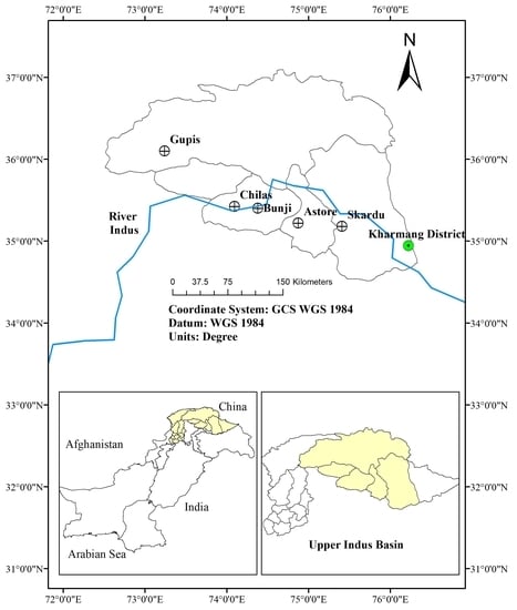
In this study, we assess spatial and temporal changes in streamflow historical data of the Indus River. Indus River gauging stations upstream of Tarbela and Kharmong dams were selected for the present study as shown in Figure 1. This study offers information for appropriate water management and planning for different sectors in the country throughout the year.
2. Data and Methods
Spatial and temporal analyses of the following time scales, temperature, and stream gauge locations were undertaken to identify statistically significant changes in flows and temperature for the study area:
- 1
- Maximum discharge
- 2
- Minimum discharge
- 3
- Mean discharge
- 4
- Maximum temperature
- 5
- Minimum temperature
Trends were observed for the overall period 1961–2010, and also by subdividing the record into two 25-year periods. Flow and temperature data from the following stations were collected from the Surface-Water Hydrology Project (SWHP), Water and Power Development Authority (WAPDA) and Pakistan Metrological Department (PMD) for the period 1961–2010. For temporal streamflow analysis, only the gauge at Tarbela is used because there is no regulation, large storage and diversion prior to that point. Also, at Tarbela a dominant portion UIB drained at that location. Climatic stations data selected for temperature analysis is covered the eastern and central Karakorum, only the Gupis represent the western Karakorum Range.
For spatial comparison, flow is analyzed from two gauging stations from 1986–2010: Tarbela and dam Kharmong. The Kharmong flow gauging station represents flows above 2550 m.a.s.l. and Tarbela represents the overall cumulative impact of the Karakorum range glaciers. Table 1 shows the elevation and time period of the data stations studied.
Daily maximum, minimum, and mean values were used to calculate the monthly maximum, minimum, and mean discharge series. Annual and seasonal means were calculated for each year. For seasonal analysis purposes, the annual water cycle was divided into two six month seasons and four three month seasons keeping in view the hydrological cycle pattern. Six month seasons were grouped as winter (October to March) and summer (April to September), whereas the three months seasons were grouped as winter (December to February), spring (March to May), summer (June to August), and autumn (September to November).
Non-parametric tests are generally distribution-free and do not require normally distributed data. They detect trend/change but do not quantify the size of the trend/change. They are very useful because most hydrologic time series data are not normally distributed. The MK test (Mann 1945; Kendall 1975) is widely adopted to assess significant trends in time series [28]. It is used to detect trends in precipitation, discharge, and temperature time series and applied in different areas including the UIB and Tibetan Plateau (TP). It is a non-parametric test, less sensitive to extreme sample values, and independent from the hypothesis about the nature of the trend. To compute the actual slope of the trend (change per year), Sen’s nonparametric procedure was used. Sen’s estimator of the slope is the median of these N values of discharge (Q). The median of the N slope estimates was obtained in the usual way; N values of Qi are ranked from smallest to largest and computed with Sen’s estimator as follows:
If N was odd
And If N was even
Data were processed using an Excel macro named MAKESENS, created by Salmi [28].
2.1. Computation of the Draught and Flood Period Indices
There are several indices that measure how much precipitation for a given period of time has deviated from historically established norms. The most commonly used for agro-ecological zoning are the following:
- Percent of normal
- Decile indices
- Palmer Drought Severity Index (PDSI)
- Surface Water Supply Index (SWSI)
Although none of the major indices is inherently superior to the rest in all circumstances, some indices are better suited than others for specific uses.
2.2. Decile Indices
The distribution of the time series of the cumulated precipitation for a given period was divided into intervals each corresponding to 10% of the total distribution (decile). Gibbs and Maher (1967) proposed to group the decile into classes of events as listed in the following table (Table 2):
3. Results and Discussion
3.1. Temperature and Discharge Trend in Annual Maximum, Minimum, and Mean Discharge
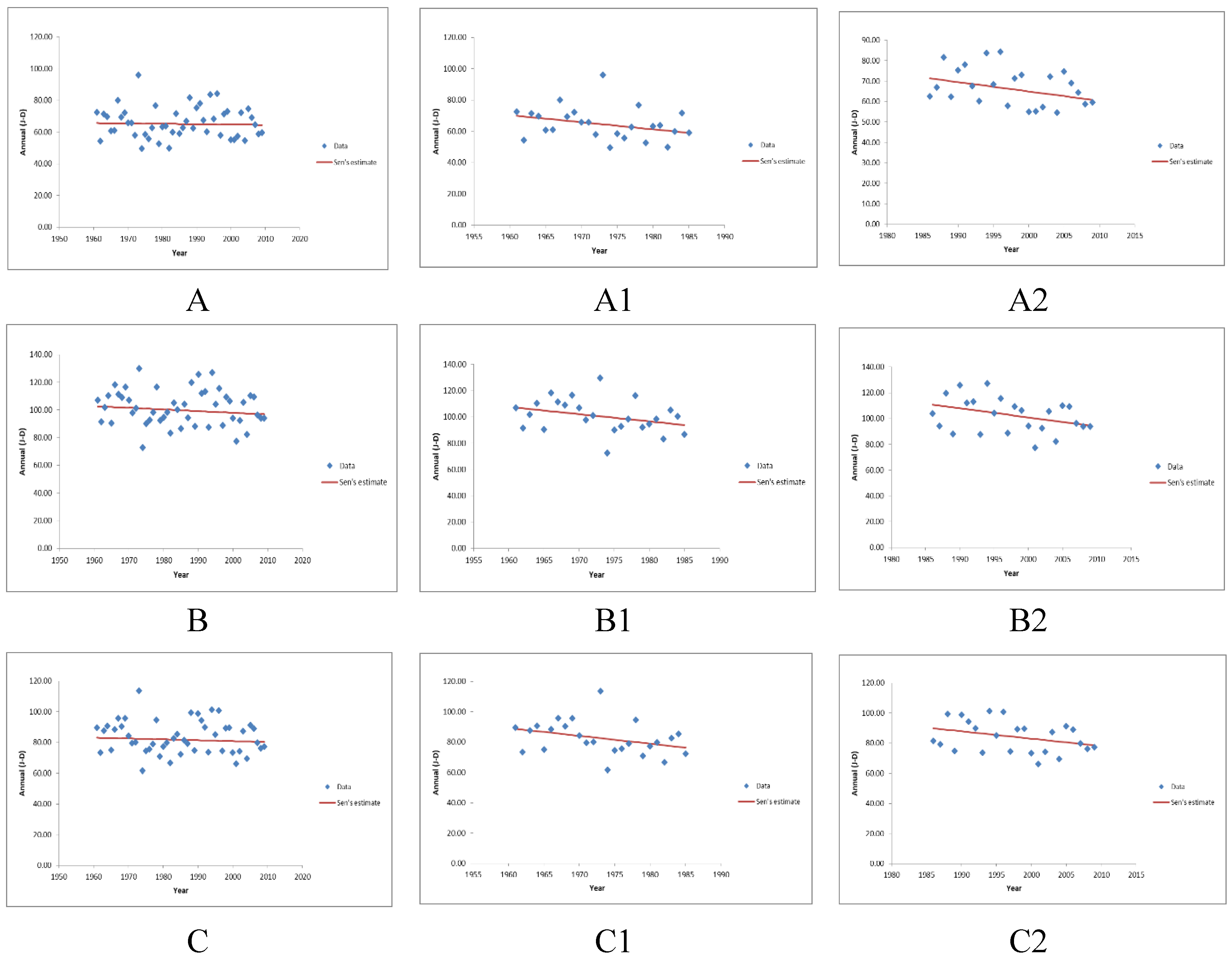
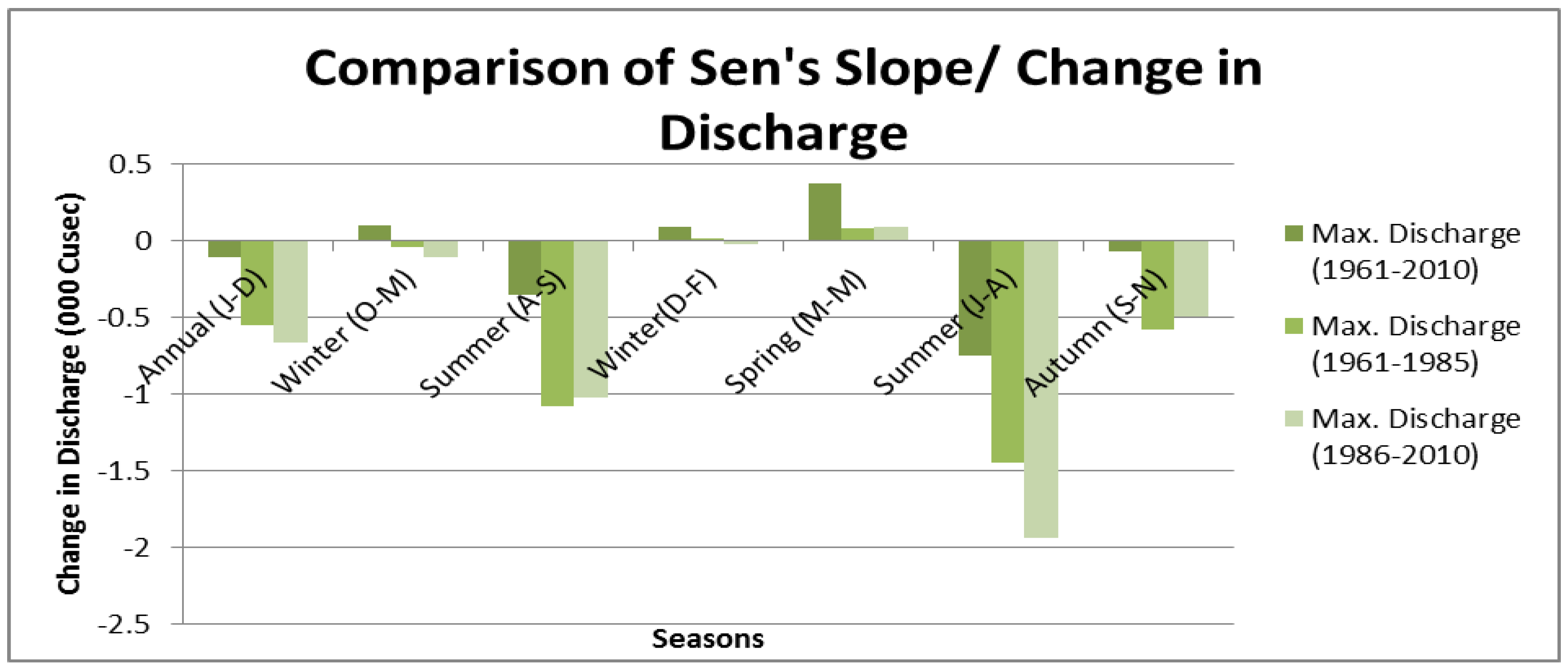
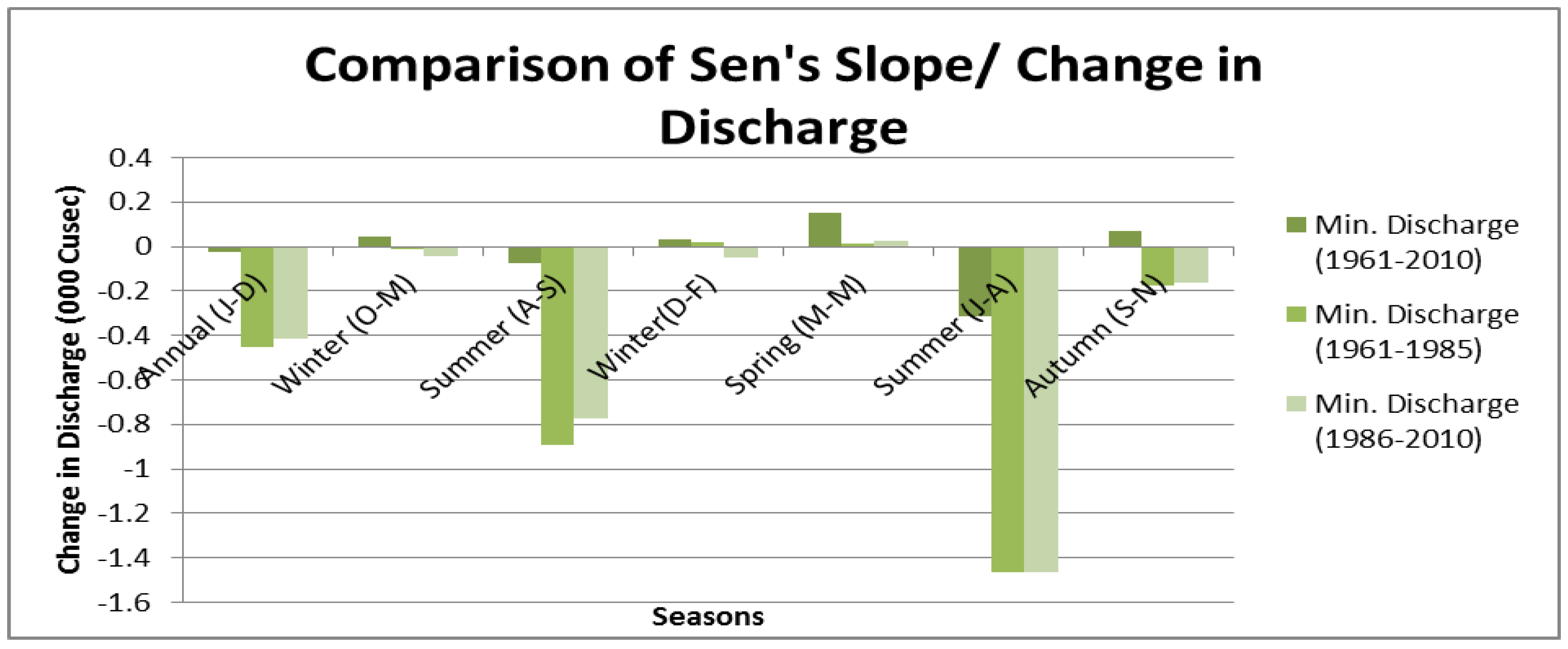
Discharge analysis of maximum, minimum, and mean discharge time series showed a decreasing trend for the period 1961–2010 (Table 3, but it is not statistically significant. Breaking the record into smaller 25 year periods, both periods show a decreasing trend, though not statistically significant. However, the maximum discharge during 1986–2010 decreased more rapidly than the 1961–1985 period as shown in Figure 2. Alternatively, minimum and mean discharges from 1961–1985 decreased more rapidly than 1986–2010. The annual maximum and minimum temperature analysis showed that there was a significant warming trend observed in the time series of 1961–2011 with more significant warming occurring from 1986–2011 as shown in Table 4. The highest warming trend for the entire record was observed at the Skardu station with 0.49 °C per decade at 99.9% significance level. The same warming trend observed at Astore, Gilgit, and Gupis stations. In contrast, the minimum temperature time series shows cooling trends at most of the climatic stations.
3.2. Discharge and Temperature Trend in Seasonal (Six Month) Maximum, Minimum, and Mean Discharge
3.2.1. Discharge and Temperature Trend in Winter (October–March) Maximum, Minimum, and Mean Discharge
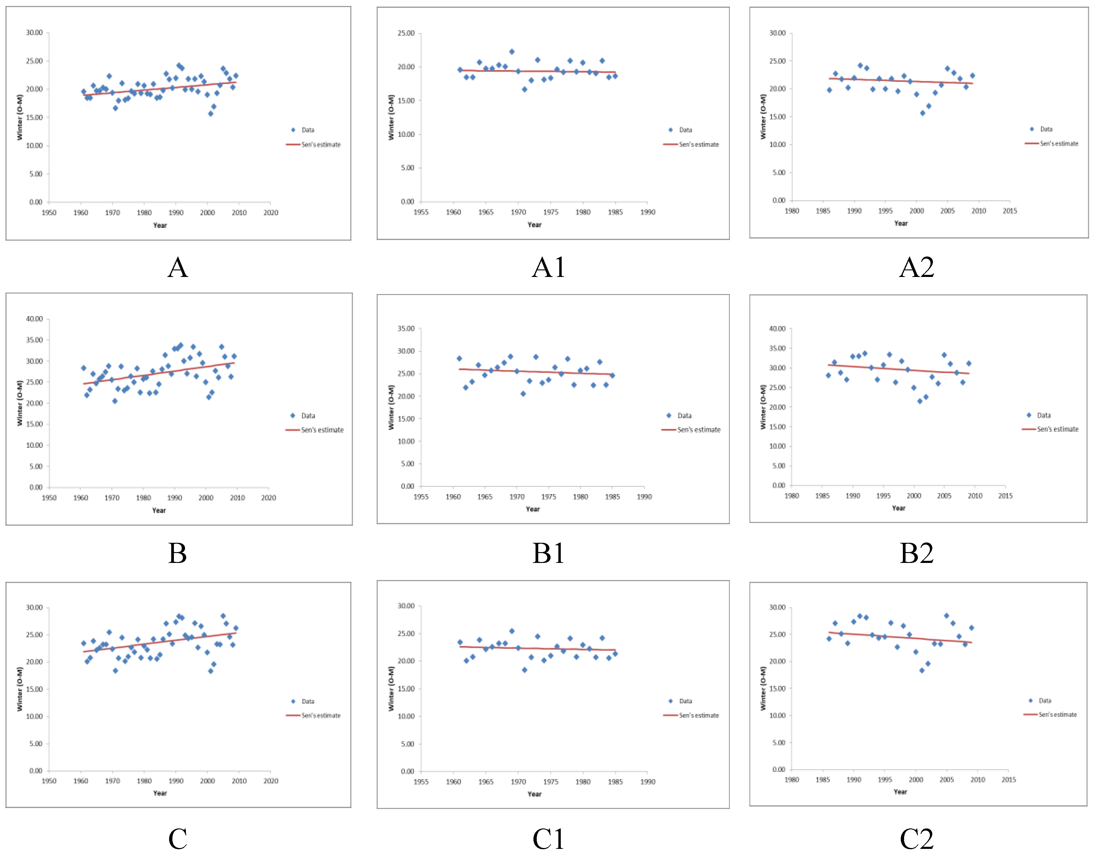
Trend analyses in maximum, minimum, and mean discharge time series showed an increase for 1961–2010 that was statistically significant at 99%, 95%, and 99% significance levels, respectively. In contrast, the smaller time intervals 1961–1985 and 1986–2010 showed decreasing trends, but these were not statistically significant, as shown in Table 3. So the overall trend was increasing, but it was decreasing when we broke it up into two time intervals as shown in Figure 3. This may be due to the irregular distribution of the wet and dry years of the natural water cycle. Flows increasing in the winter (October–March) season support studies which report climate warming in the upper Indus basin [5]. Our analysis of the temperature report similar results. Maximum temperature series for the winter month (October–March) shows a stronger warming trend compared to the annual time series. Skardu shows more warming compared to other stations. Minimum temperature series for the winter months (October–March) do not show a trend as shown in Table 5. At some stations (e.g., Bunji), the 1961–1985 record shows cooling but the 1986–2011 time period shows a warming trend. Liu et al. [29] studied 66 weather stations over the eastern and central Tibetan Plateau above the elevation of 2000 m for the time period of (1961–2013) and identified warming trends in various measures of temperature regimes, such as temperatures of extreme events as well as the diurnal temperature range. They observed that annual extreme frost days decreased during 1961–1985 and extreme warm days increased during the 1986–2013 time period.
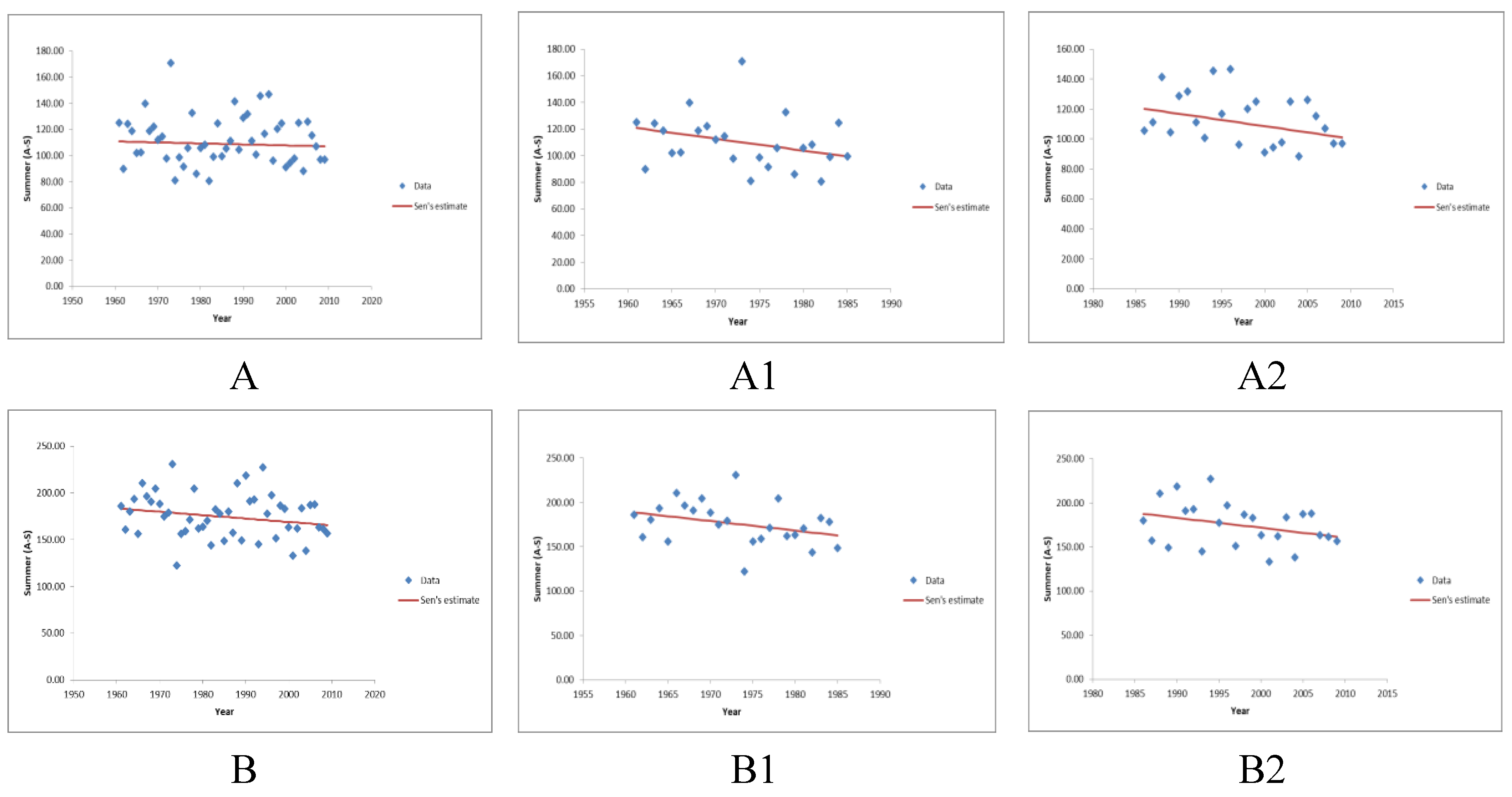
3.2.2. Discharge and Temperature Trend in Summer (April–September) Maximum, Minimum, and Mean Discharge
Summer maximum, minimum, and mean discharge time series showed a decreasing trend for all three-time intervals studied. However, these decreasing trends are not statistically significant as shown in Table 3 and Figure 4. Summer season (April–September) results align with Archer and Fowler’s [20] findings of decreased flows in the UIB. The decrease of flows at Tarbela during the summer season is also corroborated by temperature trends. It was observed that the maximum temperature series during summer (April–September) showed relatively less warm as compared to the winter (October–March) and annual (January–December) seasons. At Skardu, only 1986–2011 shows cooling trends; 1961–1985 and the entire record (1961–2011) show increasing temperature trends. The minimum temperature at Bunji, Gilgit, Gupis, and Skardu has decreased with a rate of 0.46, 0.29, 0.27, 0.39, and 0.26 °C per decade respectively at the highest significant level 99.9% as shown in the Table 6. These findings are a grave concern because this flow variation and decrease in the summer season impacted the summer season contribution in the long run in the Indus Basin for the downstream flow. More than 75–80% of Indus River flows are generated during the summer (April–September) season, a small percentage of decrease in summer results in significant reduction of flows. Pakistan’s major water consumption and withdrawal are during the summer season, and if this trend of flows continues consistently in the future, then reservoirs and other hydraulic structures’ operations must also adapt accordingly.
3.3. Discharge Trend in a Seasonal (Three Month) Maximum, Minimum, and Mean Discharge
3.3.1. Discharge Trend in Winter (December–February) Maximum, Minimum, and Mean Discharge
Discharge analysis of the three-month season for winter (December–February) aligns with the six-month winter (October–March) pattern. Again, maximum, minimum, and mean discharge time series showed increasing trends for 1961–2010 and more importantly this increase was statistically significant at 99.9%, 95%, and 99.9% significance level. From 1961–1985, flows show a slightly increasing trend. In contrast, 1986 showed a decrease in trend, though not statistically significant as (Table 3 and Figure 5, Figure 6 and Figure 7). Both winter seasons (i.e., six and three months winter seasons) showed increasing trends in discharge, which confirms studies reporting warming temperatures in low and medium elevation areas of the UIB, especially the eastern and central Karakoram regions.
3.3.2. Discharge Trend in Spring (March–May) Maximum, Minimum, and Mean Discharge
Analysis of maximum, minimum, and mean discharge showed increasing trends for 1961–2010, 1961–1985 and 1986–2010 time intervals. The overall 1961–2010 increasing trends were statistically significant, whereas the shorter 25 year time intervals were not. As we know, the spring season consists of the months of March, April, and May of the annual water cycle. As our results reveal, the spring season showed an increasing trend in line with the winter months (December–February), indicating flow contributions during the months of April and May are also increasing. As mentioned in Section 3.2.2, the summer six-month season (April–September) flows show a decreasing trend that is not statistically significant; this might be due to the April and May increasing trends. The three-month seasonal analysis also reveals that annual and six-month splitting of the water cycle does not properly capture the seasonal variations of flow in the Indus River. For optimal reservoir operation a sub-annual analysis is necessary to gauge changes in water availability throughout the year.
3.3.3. Discharge Trend in Summer (June–August) Maximum, Minimum, and Mean Discharge
Throughout the UIB, summer streamflow dominates the hydrograph. The Indus River contribution to UIB flows is significant, around 44% annually. However, during the summer season (June–August), this contribution increases to 60–65%. Table 3 shows that summer (June–August) maximum, minimum, and mean flows were decreasing—all statistically significant, for both the overall flow record as well as the 25 year intervals.
3.3.4. Discharge Trend in Autumn (September–November) Maximum, Minimum, and Mean Discharge
Analysis of autumn season maximum, minimum, and mean discharge showed decreasing trends for all observed time periods, except for an increasing minimum discharge trend for the 1961–2010 time interval. Although Sen’s equation estimates negative slope, none of the decreasing trends are statistically significant, except mean discharge for 1986–2010.
3.4. Spatial Analysis of the Indus at Kharmong and Tarbela
For spatial analysis of flow variation in the Indus River, two gauging stations were selected: Kharmong and Tarbela inflow. Historic data analysis from the 1986–2010 time period was analyzed and comparisons were also made about the flow regimes. Kharmong gauging station situated in Kharmong district at 34° 56′ 0″ latitude and 76° 13′ 0″ longitude representing 67,858 sq. km catchment area in Gilgit Baltistan. This gauging station represents the high elevation (2542 m) flow regime behavior. The Upper Indus Basin is comprised of sixteen major sub-basins, so the results of one sub-basin’s stream do not necessarily represent the other sub-basins accurately. Different studies report the behavior of the Upper Indus Basin streams differently. For example, Tahir reported that river flow trends are increasing in Astore and decreasing in Hunza Basin [19]. Dominant streamflow contributions (e.g., snow and glacial melt compared to rainfall runoff) vary amongst basins. Data for Kharmong station is not available prior to 1985, so for comparison purposes only the time interval of 1986–2010 was compared with the Tarbela station time series.
3.4.1. Spatial Analysis of the Maximum Discharge Series
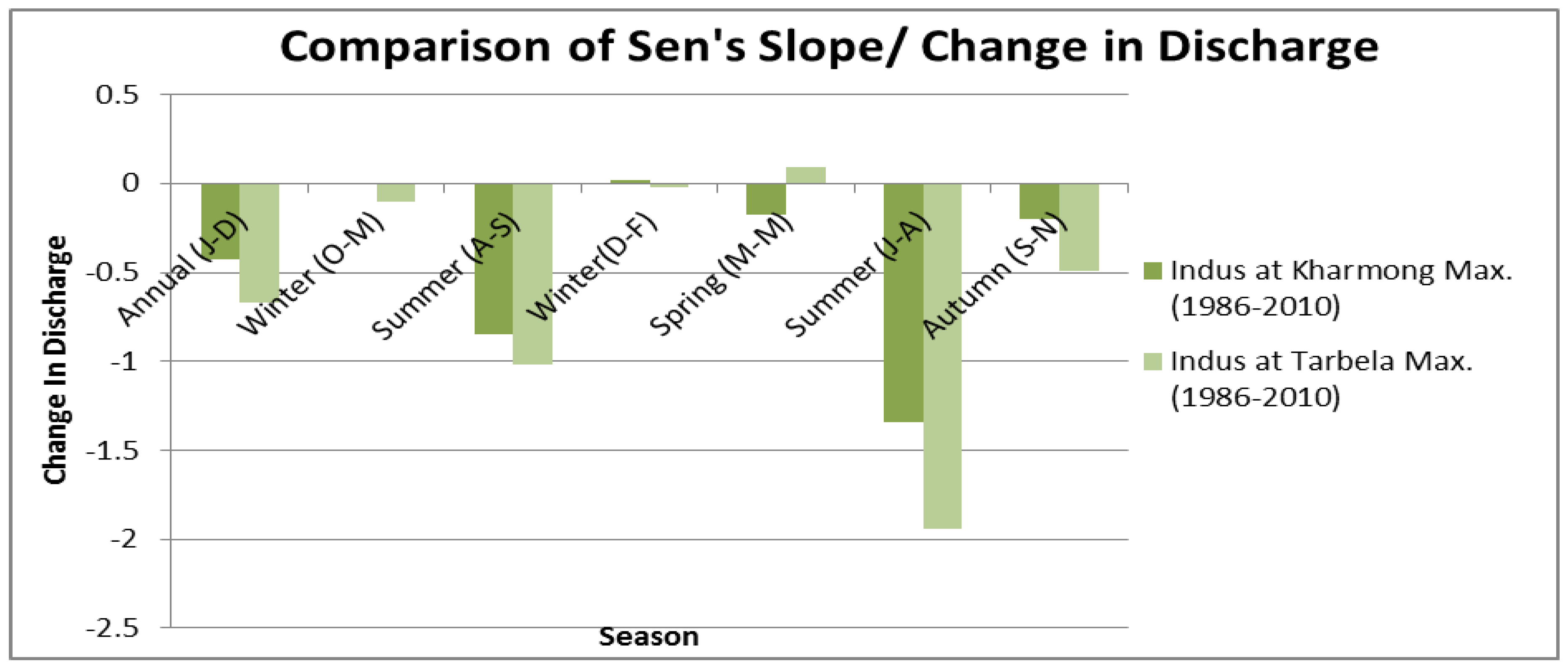
Analysis of the maximum discharge series showed that the Indus flow peaks at Kharmong station were decreasing with more statistical significance compared to the Tarbela inflow gauging station. Annual (January–December), summer (April–September), monsoon (June-August) and autumn (September–November) Sen’s Slope value was decreasing at 95%, 95%, 99% and 95% significance level, respectively, as shown in Table 7 and Figure 8, Figure 9 and Figure 10.
3.4.2. Spatial Analysis of the Minimum Discharge Series
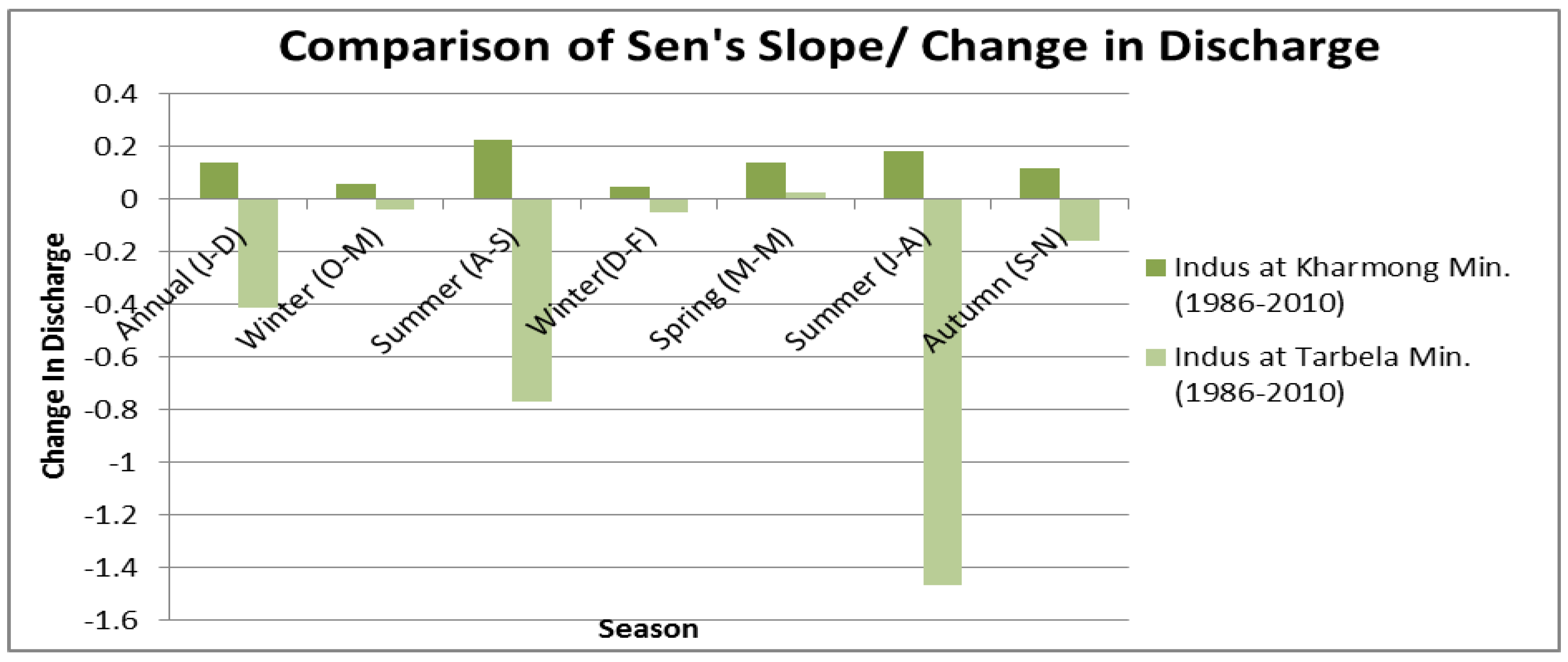
Interestingly, the minimum discharge series showed entirely different behavior than maximum discharge. Minimum discharge at Kharmong station showed a statistically significant increasing trend in discharge, compared to a decreasing trend at Tarbela gauging station. At Kharmong, annual, winter, spring, and autumn seasons showed significantly increasing trends at 90%, 99.9%, 99%, 95%, and 95% confidence levels. Minimum discharge increases, indicate that flow contribution in the low-flow periods is increasing successively possibly due to the climate warming in the area. Minimum temperature for the same time period also showed statistically significant increasing trend at Astore, Gilgit, Chilas and Bunji. Flow regime behavior at Kharmong gauging station supports the argument of overall warming at high elevation.
3.4.3. Spatial Analysis of the Mean Discharge Series
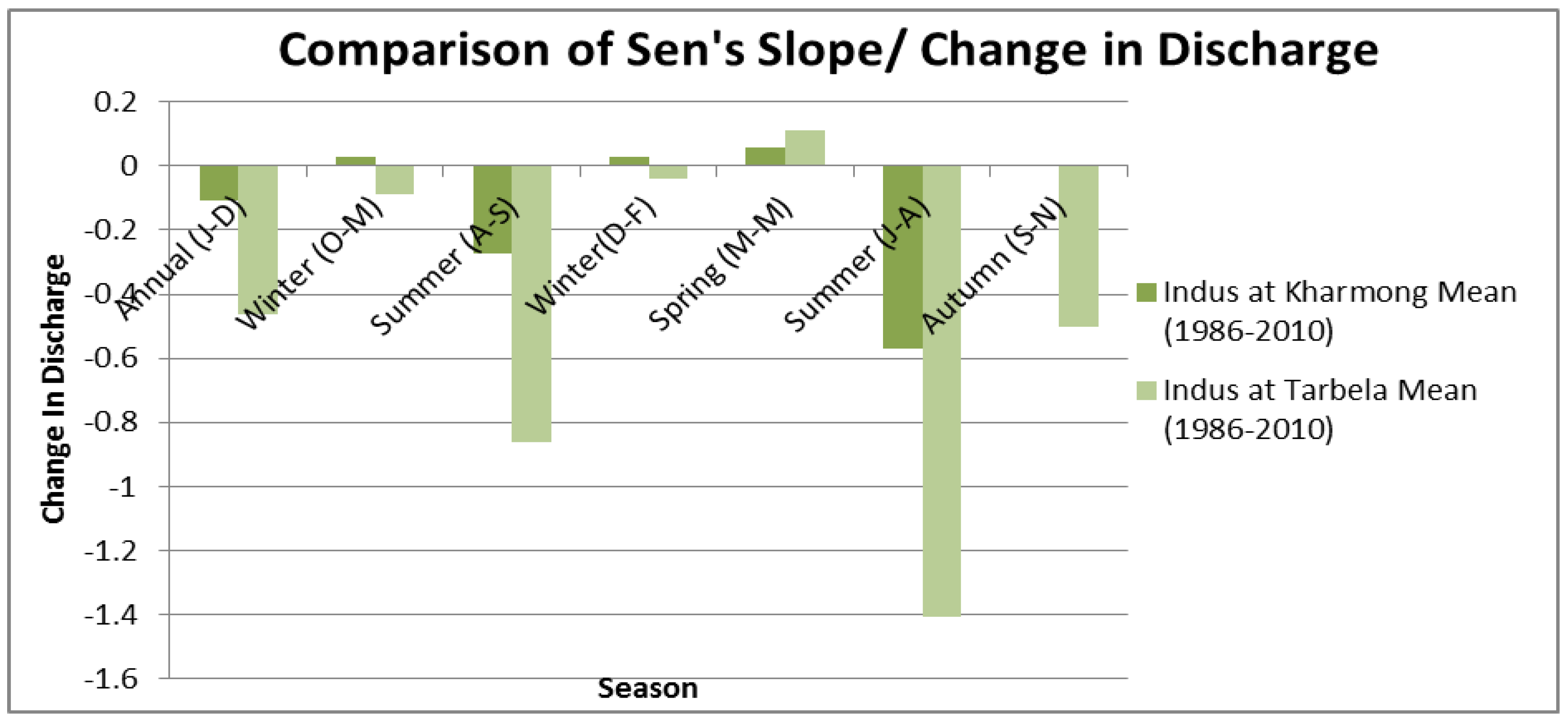
Analysis of the mean discharge showed mixed behavior compared to the maximum and minimum discharge series. Mean discharge at Kharmong during winter and spring season showed increasing trends whereas the summer season showed a decreasing trend as shown in Table 7 and Figure 8, Figure 9 and Figure 10.
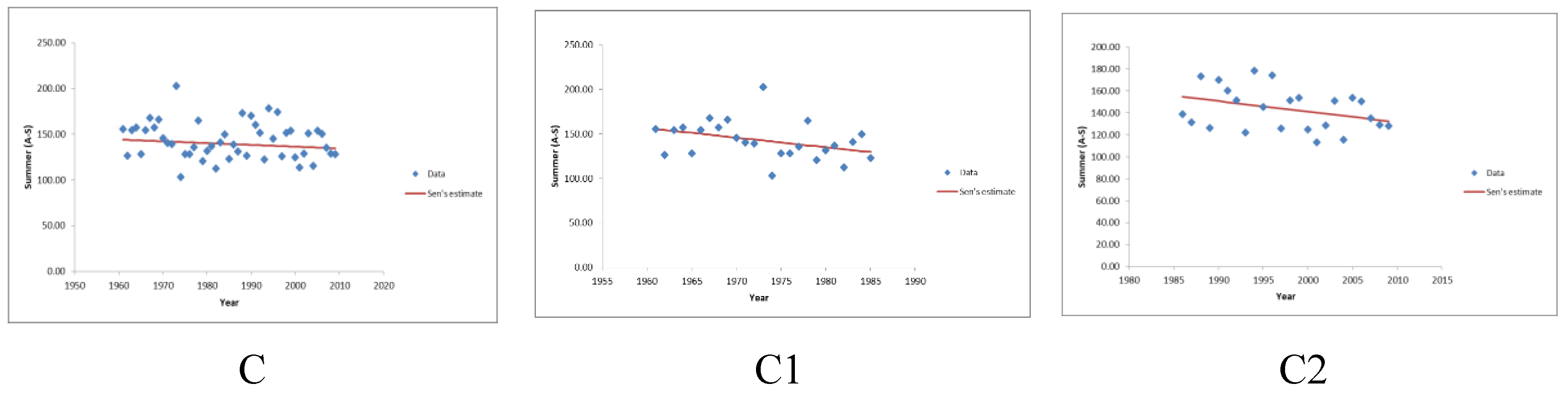
3.5. Drought and Flood Period Analysis
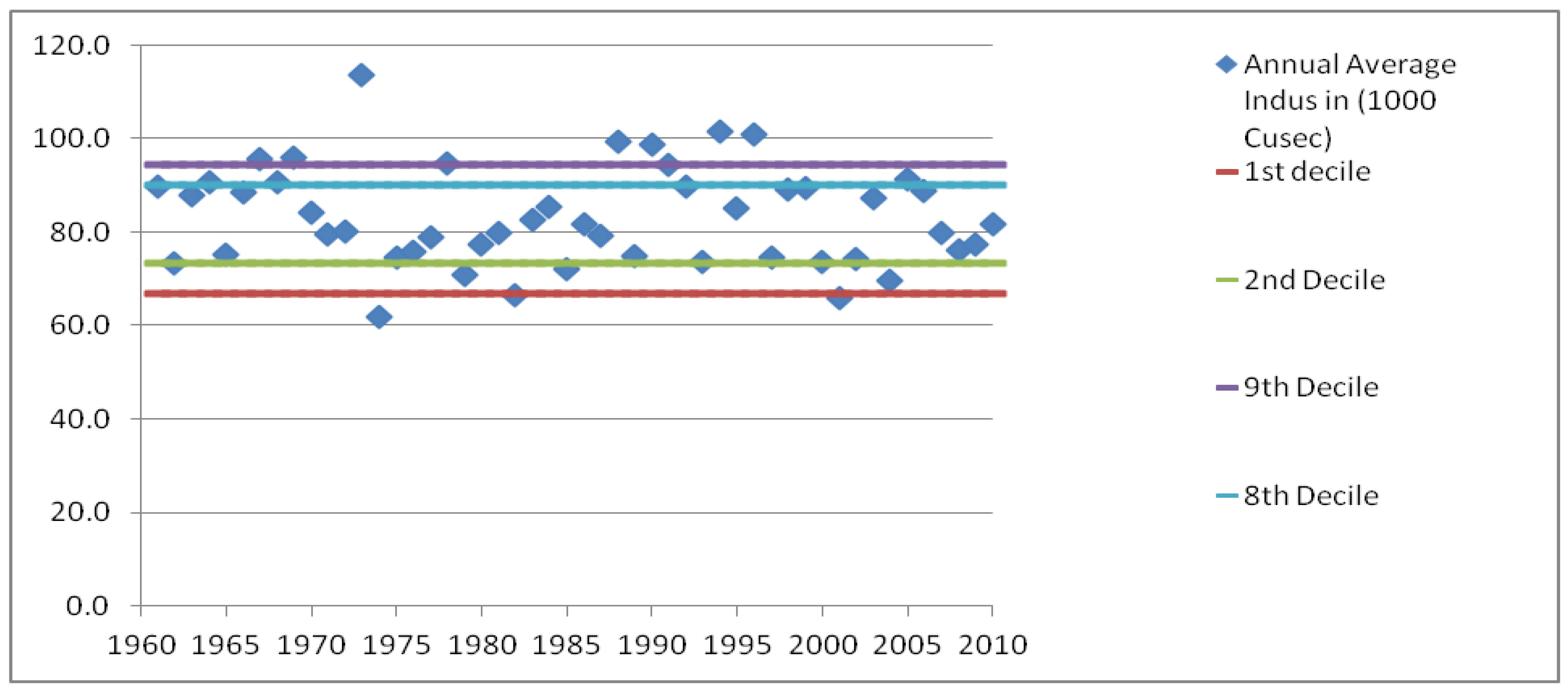
Drought and flooding period analysis was performed using the decile indices technique. The decile technique first arranges the data separately in ascending order and then divides them into 10% deciles, resulting in ten categories. Decile 1-2 is designated as “drought periods” in the data, and decile 9-10 is designated as “flood periods” in the data, i.e., values in this decile range are significantly above the mean value. Figure 11 shows drought and flood periods on the Indus River for the full 1961–2010 record. Each decade in the record shows periods assigned to both drought and also flooding, although there is no clear-cut cyclic pattern. To investigate patterns in discharge, a long-term discharge time series is required.
4. Discussion
A study [30] of the Indus River at Besham Qila (upstream of Tarbela) observed increasing flows with a rate of 6%. Sharif et.al. (2014) also studied the Besham flows from 1969–1995 and found an increasing trend [30]. In contrast, Archer and Fowler (2004) reported a decreasing trend of flows in the Indus River from the last two decades.
Minimum flows increasing at the Kharmong gauging site support the argument of [7] of significant warming on the Tibetan Plateau. Liu and Chen [13] also studied temperature trends over the entire TP and found that temperatures increase linearly from 1955–1996. They report a 0.16 C0/decade increase in annual mean temperatures, whereas the winter season mean increased 0.32 C0/decade. Otherwise, readers will likely attribute the quote to Duan and Xiao “In contrast to the cooling trend in the rest of China, and the global warming hiatus post-1990s, an accelerated warming trend has appeared over the Tibetan Plateau during 1998–2013 (0.25 °C decade−1), compared with that during 1980–1997 (0.21 °C decade−1)” [31] (p. 1).
Recently [32] studied temperature trends for the time period 1961–2012 and reported a warming trend, which is almost double the previously reported figure. It was also noted that a warming trend was found to be significant in the minimum temperatures series, compared to the maximum temperatures. [33] reported that frequency of cold days and nights decreased −0.85 and −2.38/decade, respectively, whereas, the frequency of hot days and nights increased 1.26 and 2.54 per decade respectively. Our conclusions for winter and spring seasons minimum discharge trends at Kharmong as well as Tarbela gauging stations match and support the above cited findings. At Tarbela gauging station all three discharge series, i.e., maximum, minimum, and mean discharge increased significantly, which supports the argument of warming over the Upper Indus Basin (UIB) and its accumulative impact shown in the discharge trend for winter and spring season.
Different studies [34,35] reported that the rate of warming is more significant at high elevations. Our comparison of Kharmong and Tarbela inflows also provides insight about this significant elevation-dependent warming.
Mukhopadhyay reports a reduction of about 2.15% in snow and ice extent between 1992 and 2010. The Indus flows at Tarbela and Kharmong during almost the same periods, 1986–2010, demonstrated summer discharges were significantly decreasing, and maximum/peaks also decreased significantly. Archer and Fowler [17,20] concluded that river flows were reduced between (1894–1994) due to the positive glacier mass balance in the UIB. Our results reveal that, for the winter and spring seasons, streamflow has increased significantly, whereas for summer and autumn seasons it has decreased significantly. There are varied potential interpretations of these flow dynamics. One possibility is that winter and summer seasons temperature warming increases the melt rate so a decrease in summer flows could be partly due to cooler temperatures, but it could also be partly due to increased melt in the winter months resulting in less snow available to melt in the summer months. This loss of mass in the winter precludes the simple conclusion that decreased flows in the summer show a sign of positive mass balance. Although there is glacial stability or even advancement in some basins as reported in the studies [17,20,21], we cannot extrapolate this phenomenon over the entire UIB and further investigation is necessary.
5. Conclusions and Recommendations
Flow variation shows greater magnitude seasonally rather than annually. Quantifying this variation is important for water resources management downstream for flood mitigation and also to plan proper withdrawal/storage. Winter and spring season discharges are increasing, whereas summer and autumn discharges are decreasing in all discharge data series at Tarbela gauging station. Minimum discharge is increasing at higher elevations, i.e., Kharmong, and decreasing at the lower elevation point, Tarbela, whereas maximum and mean discharges show decreasing trends at both gauging sites (with Tarbela decreasing more significantly). The period 2000–2004 shows the lowest flows during the study period of 1961–2010. Reduction of flows in the summer season (implying glacier storage) coupled with increases in the winter (connoting glacier mass loss) provides insight into the complexity of glacial status and the water balance in the Karakoram Mountains, for which spirited debate still continues.
Following are the Recommendations
- More flow gauging data for the UIB streams analysis is required for any definite conclusion.
- The co-relation of temperature and precipitation parameters with the flow yields more insights into the hydrological phenomenon of the basin.
- The accuracy of discharge measurement needs to be examined at the gauging site for refinement of this analysis.
Author Contributions
Conceptualization, M.A.; methodology, M.A. and D.H.; software, A.A. and D.H.; validation, M.A. and A.A. data curation, M.S. and D.H.; writing—original draft preparation, M.A.; writing—review and editing, J.L.; visualization, D.H.; supervision, M.A.
Funding
This research received no external funding.
Conflicts of Interest
The authors declare no conflict of interest.
References
- Arfan, M.; Makhdum, A.H.; Nabi, G. Assessment of temporal flow variability of the Kabul River. J. Moun. Area Res. 2016, 2, 1–8. [Google Scholar]
- Bolch, T.; Kulkarni, A.; Kääb, A.; Huggel, C.; Paul, F.; Cogley, J.G.; Frey, H.; Kargel, J.S.; Fujita, K.; Scheel, M.; et al. The State and Fate of Himalayan Glaciers. Science 2012, 336, 310–314. [Google Scholar] [CrossRef] [PubMed] [Green Version]
- Folland, C.K.; Karl, T.R.; Christy, J.R.; Clarke, R.A.; Gruza, G.V.; Jouzel, J.; Mann, M.E.; Oerlemans, J.; Salinger, M.J.; Wang, S.-W. Climate Change 2001: The Scientific Basis. Contribution of Working Group I to the Third Assessment Report of the Intergovernmental Panel on Climate Change; Cambridge University Press: Cambridge, UK, 2001; 881. [Google Scholar]
- Morgan, K. Researchers resolve the Karakoram glacier anomaly, a cold case of climate science. Princet. Univ. 2014, 39–41. [Google Scholar]
- You, Q.-L.; Ren, G.-Y.; Zhang, Y.-Q.; Ren, Y.-Y.; Sun, X.-B.; Zhan, Y.-J.; Shrestha, A.B.; Krishnan, R. An Overview of Studies of Observed Climate Change in the Hindu Kush Himalayan (HKH) Region. Adv. Clim. Chang. Res. 2017, 8, 141–147. [Google Scholar] [CrossRef]
- Barnett, T.P.; Adam, J.C.; Lettenmaier, D.P. Potential Impacts of a Warming Climate on Water Availability in Snow-Dominated Regions. Nature 2005, 438, 303–309. [Google Scholar] [CrossRef] [PubMed]
- Kang, S.; Xu, Y.; You, Q.; Flügel, W.-A.; Pepin, N.; Yao, T. Review of climate and cryospheric change in the Tibetan Plateau. Environ. Res. Lett. 2010, 5, 015101. [Google Scholar] [CrossRef]
- Pepin, N.; Bradley, R.S.; Diaz, H.F.; Baraer, M.; Caceres, E.B.; Forsythe, N.; Fowler, H.; Greenwood, G.; Hashmi, M.Z.; Liu, X.D.; et al. Elevation Dependent Warming in Mountain Regions of the World. Nat. Clim. Chang. 2015, 5, 424–430. [Google Scholar]
- Qiu, J. China: The third pole. Nature 2008, 454, 393–396. [Google Scholar] [CrossRef] [Green Version]
- Sarıkaya, M.A.; Bishop, M.P.; Shroder, J.F.; Ali, G.; Sarikaya, M.A. Remote-sensing assessment of glacier fluctuations in the Hindu Raj, Pakistan. Int. J. Sens. 2013, 34, 3968–3985. [Google Scholar] [CrossRef]
- Mukhopadhyay, B. Detection of dual effects of degradation of perennial snow and ice covers on the hydrologic regime of a Himalayan river basin by stream water availability modeling. J. Hydrol. 2011, 412–413, 14–33. [Google Scholar] [CrossRef]
- Prasad, A.K.; Yang, K.-H.S.; El-Askary, H.; Kafatos, M. Melting of major Glaciers in the western Himalayas: Evidence of climatic changes from long term MSU derived tropospheric temperature trend (1979–2008). Ann. Geophys. 2009, 27, 4505–4519. [Google Scholar] [CrossRef]
- Liu, X.; Chen, B. Climatic warming in the Tibetan Plateau during recent decades. Int. J. Clim. 2000, 20, 1729–1742. [Google Scholar] [CrossRef]
- Wang, W.; Xiang, Y.; Gao, Y.; Lu, A.; Yao, T. Rapid expansion of glacial lakes caused by climate and glacier retreat in the Central Himalayas. Hydrol. Process. 2015, 29, 859–874. [Google Scholar] [CrossRef]
- Ming, J. Widespread albedo decreasing and induced melting of Himalayan snow and ice in the early 21st century. PLoS ONE 2015, 10, 1–20. [Google Scholar] [CrossRef] [PubMed]
- Oerlemans, J. Extracting a Climate Signal from 169 Glacier Records. Science 2005, 308, 675–677. [Google Scholar] [CrossRef] [PubMed] [Green Version]
- Hewitt, K. The Karakoram Anomaly? Glacier Expansion and the ‘Elevation Effect,’ Karakoram Himalaya. Mt. Res. Dev. 2005, 25, 332–340. [Google Scholar] [CrossRef]
- Zhao, L.; Ding, R.; Moore, J.C. Glacier volume and area change by 2050 in high mountain Asia. Glob. Planet. Chang. 2014, 122, 197–207. [Google Scholar] [CrossRef]
- Tahir, A.A.; Chevallier, P.; Arnaud, Y.; Ashraf, M.; Bhatti, M.T. Snow cover trend and hydrological characteristics of the Astore River basin (Western Himalayas) and its comparison to the Hunza basin (Karakoram region). Sci. Total. Environ. 2015, 505, 748–761. [Google Scholar] [CrossRef] [PubMed]
- Archer, D.R.D.; Fowler, H.J.H. Spatial and temporal variations in precipitation in the Upper Indus Basin, global teleconnections and hydrological implications. Hydrol. Earth Sys. Sci. 2004, 8, 47–61. [Google Scholar] [CrossRef] [Green Version]
- Gardelle, J.; Berthier, E.; Arnaud, Y. Slight mass gain of Karakoram glaciers in the early twenty-first century. Nat. Geosci. 2012, 5, 322–325. [Google Scholar] [CrossRef]
- Jacob, T.; Wahr, J.; Pfeffer, W.T.; Swenson, S. Recent contributions of glaciers and ice caps to sea level rise. Nature 2012, 482, 514–518. [Google Scholar] [CrossRef] [PubMed]
- Matsuo, K.; Heki, K. Time-variable ice loss in Asian high mountains from satellite gravimetry. Earth Planet. Sci. Lett. 2010, 290, 30–36. [Google Scholar] [CrossRef]
- Qiu, J. Glaciologists to target third pole. Nature 2012, 484, 19. [Google Scholar] [CrossRef]
- Scherler, D.; Bookhagen, B.; Strecker, M.R. Spatially variable response of Himalayan glaciers to climate change affected by debris cover. Nat. Geosci. 2011, 4, 156–159. [Google Scholar] [CrossRef]
- Khan, A.; Richards, K.S.; Parker, G.T.; McRobie, A.; Mukhopadhyay, B. How large is the Upper Indus Basin? The pitfalls of auto-delineation using DEMs. J. Hydrol. 2014, 509, 442–453. [Google Scholar] [CrossRef]
- Bamber, J. Climate change: Shrinking glaciers under scrutiny. Nature 2012, 482, 482–483. [Google Scholar] [CrossRef]
- Bocchiola, D.; Diolaiuti, G. Recent (1980–2009) evidence of climate change in the upper Karakoram, Pakistan. Theor. App. Climatol. 2013, 113, 611–641. [Google Scholar] [CrossRef]
- Liu, X.; Yin, Z.-Y.; Shao, X.; Qin, N. Temporal trends and variability of daily maximum and minimum, extreme temperature events, and growing season length over the eastern and central Tibetan Plateau during 1961–2003. J. Geophys. Res. Biogeosci. 2006, 111. [Google Scholar] [CrossRef]
- Ahsan, M.; Shakir, A.S.; Zafar, S.; Nabi, G.; Ahsan, E.M. Assessment of Climate Change and Variability in Temperature, Precipitation and Flows in Upper Indus Basin. Int. J. Sci. Eng. Res. 2016, 7, 1610–1620. [Google Scholar]
- Duan, A.; Xiao, Z. Does the climate warming hiatus exist over the Tibetan Plateau? Sci. Rep. 2015, 5, 1–9. [Google Scholar] [CrossRef]
- Yan, L.; Liu, X. Has Climatic Warming over the Tibetan Plateau Paused or Continued in Recent Years? J. Earth Ocean Atmos. Sci. 2014, 1, 13–28. [Google Scholar]
- You, Q.; Kang, S.; Aguilar, E.; Yan, Y. Changes in daily climate extremes in the eastern and central Tibetan Plateau during 1961–2005. J. Geophys. Res. Biogeosci. 2008, 113, 1–17. [Google Scholar] [CrossRef]
- You, Q.; Kang, S.; Pepin, N.; Flügel, W.-A.; Yan, Y.; Behrawan, H.; Huang, J. Relationship between Temperature Trend Magnitude, Elevation and Mean Temperature in the Tibetan Plateau from Homogenized Surface Stations and Reanalysis Data. Glob. Planet. Chang. 2010, 71, 124–133. [Google Scholar] [CrossRef]
- You, Q.; Kang, S.; Pepin, N.; Yan, Y. Relationship between trends in temperature extremes and elevation in the eastern and central Tibetan Plateau, 1961–2005. Geophys. Res. Lett. 2008, 35, 1–7. [Google Scholar] [CrossRef]
Figure 1.
Location map of the discharge and temperature data station in the study area.

Figure 2.
Discharge trend in annual (January-December); minimum, maximum, and mean time series. First row showing trend (A,A1,A2) minimum discharge series trend for 1961–2010, 1961–1985, and 1986–2010 time interval respectively. Second (B,B1,B2) and third (C,C1,C2) row showing maximum and mean discharge series trend.

Figure 3.
Discharge trend in winter (October–March); minimum, maximum, and mean time series. First row showing trend (A,A1,A2) minimum discharge series trend for 1961–2010, 1961–1985 and 1986–2010 time interval respectively. Second (B,B1,B2) and third (C,C1,C2) row showing maximum and mean discharge series trend.

Figure 4.
Discharge trend in summer (April–September); minimum, maximum, and mean time series. First row showing trend (A,A1,A2) minimum discharge series trend for 1961–2010, 1961–1985, and 1986–2010 time intervals respectively. Second (B,B1,B2) and third (C,C1,C2) rows showing maximum and mean discharge series trend.


Figure 5.
Comparison of change in maximum discharge.

Figure 6.
Comparison of change in minimum discharge.

Figure 7.
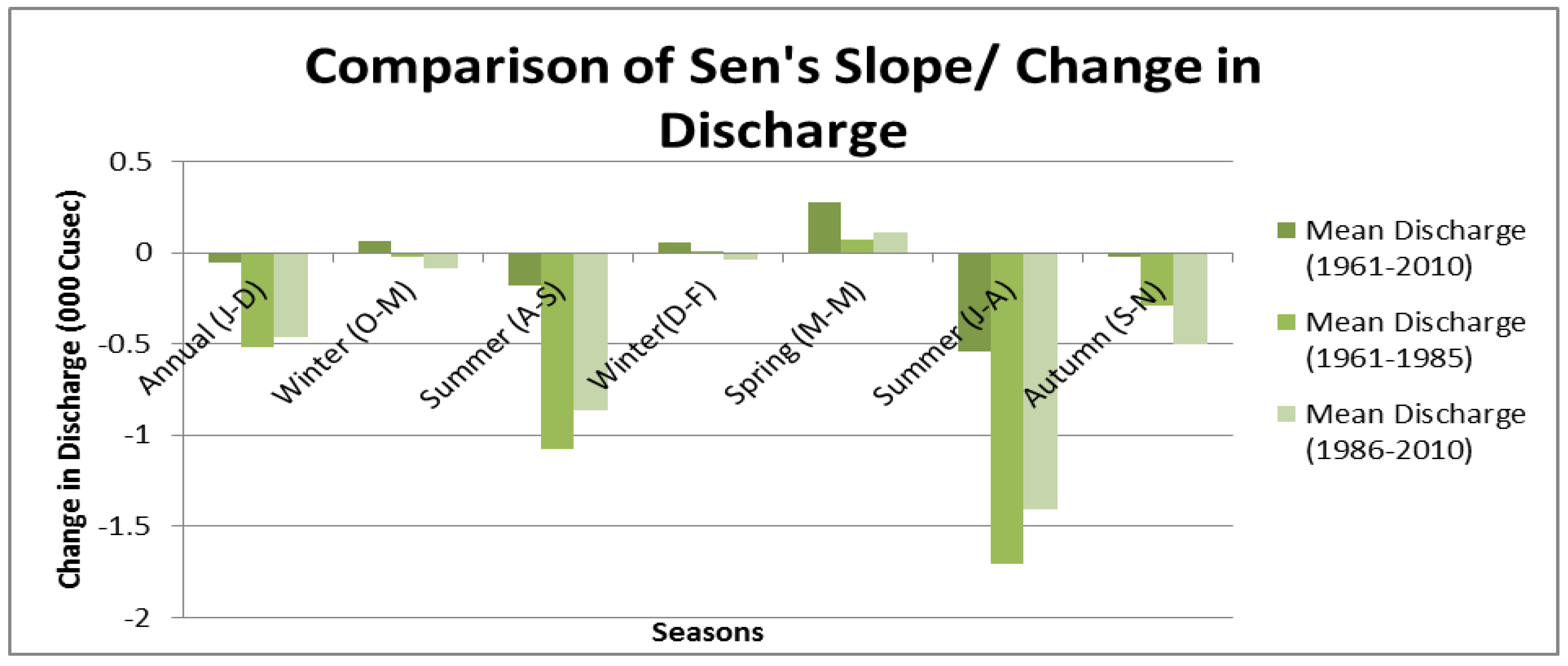
Comparison of change in mean discharge.

Figure 8.
Comparison of change in maximum discharge.

Figure 9.
Comparison of change in minimum discharge.

Figure 10.
Comparison of change in mean discharge.

Figure 11.
Comparison of draught and flood periods.


Table 1.
Data stations with their time periods.
| Name of Station | Type of Data | Elevation a.m.s.l (m) | Time Period |
|---|---|---|---|
| Kharmong | Discharge | 2542 | 1986–2010 |
| Tarbela Inflow | Discharge | 442 | 1961–2010 |
| Astore | Temperature | 2168 | 1961–2011 |
| Bunji | Temperature | 1372 | 1961–2011 |
| Chilas | Temperature | 1250 | 1961–2011 |
| Gilgit | Temperature | 1460 | 1961–2011 |
| Gupis | Temperature | 2156 | 1961–2011 |
| Skardu | Temperature | 2317 | 1961–2011 |
Table 2.
Decile drought classification classes.
| Class | Percent | Category |
|---|---|---|
| Decile 1–2 | 20% lower | much below normal |
| Decile 3–4 | 20% following | below normal |
| Decile 5–6 | 20% medium | near normal |
| Decile 7–8 | 20% following | above normal |
| Decile 9–10 | 20% high | much above normal |
Table 3.
Trends in annual maximum, minimum, and mean discharge of Indus River (Tarbela Inflow) for period (1961–2010) and 25 year time interval showing discharge change in 1000 Cusec/decade.
Table 3.
Trends in annual maximum, minimum, and mean discharge of Indus River (Tarbela Inflow) for period (1961–2010) and 25 year time interval showing discharge change in 1000 Cusec/decade.
| Discharge Change (1000 Cusec) | |||||||||
|---|---|---|---|---|---|---|---|---|---|
| Maximum Discharge | Minimum Discharge | Mean Discharge | |||||||
| Season | 1961–2010 | 1961–1985 | 1986–2010 | 1961–2010 | 1961–1985 | 1961–1986 | 1961–2010 | 1961–1985 | 1986–2010 |
| Annual (J-D) | −0.112 | −0.552 | −0.669 | −0.023 | −0.453 | −0.412 | −0.056 | −0.519 | −0.462 |
| Winter (O-M) | 0.095 ** | −0.046 | −0.104 | 0.044 * | −0.009 | −0.042 | 0.063 ** | −0.024 | −0.088 |
| Summer (A-S) | −0.357 | −1.079 | −1.02 | −0.072 | −0.893 | −0.771 | –0.179 | −1.08 + | −0.863 |
| Winter (D-F) | 0.085 *** | 0.018 | −0.022 | 0.032 * | 0.022 | −0.052 | 0.052 ** | 0.01 | −0.039 |
| Spring (M-M) | 0.375 *** | 0.078 | 0.094 | 0.149 * | 0.012 | 0.027 | 0.277 *** | 0.07 | 0.11 |
| Summer (J-A) | −0.753 * | −1.45 + | −1.94 + | −0.315 | −1.465 | −1.46 + | −0.543 + | −1.70 + | −1.408 |
| Autumn (S-N) | −0.071 | −0.584 | −0.493 | 0.072 | −0.178 | −0.161 | −0.022 | −0.289 | −0.50 + |
*** Significance level ≤99.9%, ** Significance level ≤99%. * Significance level ≤95%. + Significance level ≤90%. Bold = Significant Negative Trend.
Table 4.
Mean maximum and minimum annual (January–December) temperature change/decade (°C).
| Stations | Maximum Temperature | Minimum Temperature | ||||
|---|---|---|---|---|---|---|
| 1961–2011 | 1961–1985 | 1986–2011 | 1961–2011 | 1961–1985 | 1986–2011 | |
| Astore | 0.21 *** | 0.01 | 0.63 *** | 0.10 * | 0.10 * | 0.64 *** |
| Bunji | −0.03 | −0.02 | 0.41 ** | −0.26 * | −0.26 * | 0.60 *** |
| Chilas | 0.01 | 0.14 | 0.44 * | 0.21 *** | 0.21 *** | 0.19 |
| Gilgit | 0.30 *** | 0.11 | 0.52 *** | −0.17 *** | −0.17 *** | 0.10 |
| Gupis | 0.22 *** | 0.30 + | 0.73 *** | −0.29 *** | −0.29 *** | −0.80 |
| Skardu | 0.49 *** | 0.54 *** | 0.14 | −0.13 *** | −0.13 *** | −0.09 |
*** Significance level ≤99.9%, ** Significance level ≤99%. * Significance level ≤95%. + Significance level ≤90%. Bold = Significant Negative Trend.
Table 5.
Mean maximum and minimum winter (October–March) temperature change/decade (°C).
| Stations | Maximum Temperature | Minimum Temperature | ||||
|---|---|---|---|---|---|---|
| 1961–2011 | 1961–1985 | 1986–2011 | 1961–2011 | 1961–1985 | 1986–2011 | |
| Astore | 0.33 *** | 0.07 | 0.72 *** | 0.17 *** | 0.17 *** | 0.58 *** |
| Bunji | 0.20 *** | 0.06 | 0.51 ** | −0.15 | −0.15 | 0.59 *** |
| Chilas | 0.16 ** | 0.29 ** | 0.65 ** | 0.35 *** | 0.35 *** | 0.40 * |
| Gilgit | 0.45 *** | 0.13 | 0.85 *** | 0.001 | 0.001 | 0.02 |
| Gupis | 0.34 *** | 0.44 * | 0.92 *** | −0.18 | −0.18 | −0.96 |
| Skardu | 0.66 *** | 0.31 + | 0.54 ** | 0.01 | 0.01 | −0.12 |
*** Significance level ≤99.9%, ** Significance level ≤99%. * Significance level ≤95%. + Significance level ≤90%. Bold = Significant Negative Trend.
Table 6.
Mean maximum and minimum Summer (April–September) temperature change/decade (°C).
| Stations | Maximum Temperature | Minimum Temperature | ||||
|---|---|---|---|---|---|---|
| 1961–2011 | 1961–1985 | 1986–2011 | 1961–2011 | 1961–1985 | 1986–2011 | |
| Astore | 0.11 * | 0.16 | 0.56 *** | 0.02 | 0.02 | 0.66 *** |
| Bunji | −0.25 *** | 0.001 | 0.37 * | −0.46 ** | −0.46 ** | 0.67 *** |
| Chilas | −0.07 | 0.25 | 0.24 * | 0.04 | 0.04 | 0.04 |
| Gilgit | 0.17 *** | 0.20 | 0.26 * | −0.27 *** | −0.27 *** | 0.25 |
| Gupis | 0.11 * | 0.32 * | 0.55 *** | −0.38 *** | −0.38 *** | −0.30 |
| Skardu | 0.42 *** | 0.91 *** | −0.16 + | −0.26 *** | −0.26 *** | −0.07 |
*** Significance level ≤99.9%. ** Significance level ≤99%. * Significance level ≤95%. + Significance level ≤90%. Bold = significant negative trend.
Table 7.
Comparison of the spatial variation of trends in the Indus River for the 1986–2010 time series, showing discharge change in 1000 Cusec/decade.
Table 7.
Comparison of the spatial variation of trends in the Indus River for the 1986–2010 time series, showing discharge change in 1000 Cusec/decade.
| Maximum Discharge | Minimum Discharge | Mean Discharge | ||||
|---|---|---|---|---|---|---|
| Indus at Kharmong | Indus at Tarbela | Indus at Kharmong | Indus at Tarbela | Indus at Kharmong | Indus at Tarbela | |
| Seasons | 1986–2010 | 1986–2010 | 1986–2010 | 1986–2010 | 1986–2010 | 1986–2010 |
| Annual (J-D) | −0.423 * | −0.669 | 0.141 + | −0.412 | −0.110 | −0.462 |
| Winter (O-M) | −0.008 | −0.104 | 0.066 *** | −0.042 | 0.030 + | −0.088 |
| Summer (A-S) | −0.850 * | −1.02 | 0.277 | −0.771 | −0.276 | −0.863 |
| Winter (D-F) | 0.019 | −0.022 | 0.045 ** | −0.052 | 0.026 | −0.039 |
| Spring (M-M) | −0.173 | 0.094 | 0.137 * | 0.027 | 0.059 | 0.11 |
| Summer (J-A) | −1.340 ** | −1.940 + | 0.183 | −1.463 + | −0.568 * | −1.408 |
| Autumn (S-N) | −0.203 * | −0.493 | 0.119 * | −0.161 | 0.004 | −0.503 + |
*** Significance level ≤99.9%. ** Significance level ≤99%. * Significance level ≤95%. + Significance level ≤90%. Bold = Significant Negative Trend.
© 2019 by the authors. Licensee MDPI, Basel, Switzerland. This article is an open access article distributed under the terms and conditions of the Creative Commons Attribution (CC BY) license (http://creativecommons.org/licenses/by/4.0/).
Share and Cite
MDPI and ACS Style
Arfan, M.; Lund, J.; Hassan, D.; Saleem, M.; Ahmad, A. Assessment of Spatial and Temporal Flow Variability of the Indus River. Resources 2019, 8, 103. https://0-doi-org.brum.beds.ac.uk/10.3390/resources8020103
AMA Style
Arfan M, Lund J, Hassan D, Saleem M, Ahmad A. Assessment of Spatial and Temporal Flow Variability of the Indus River. Resources. 2019; 8(2):103. https://0-doi-org.brum.beds.ac.uk/10.3390/resources8020103
Chicago/Turabian StyleArfan, Muhammad, Jewell Lund, Daniyal Hassan, Maaz Saleem, and Aftab Ahmad. 2019. "Assessment of Spatial and Temporal Flow Variability of the Indus River" Resources 8, no. 2: 103. https://0-doi-org.brum.beds.ac.uk/10.3390/resources8020103
Note that from the first issue of 2016, this journal uses article numbers instead of page numbers. See further details here.