
A Novel Implementation of Siamese Type Neural Networks in Predicting Rare Fluctuations in Financial Time Series


1
Department of Mathematics, Occidental College, Los Angeles, CA 90041, USA
2
Department of Geography, University of California, Santa Barbara, CA 93117, USA
3
Department of Statistics, University of California Los Angeles, Los Angeles, CA 90095, USA
4
Department of Mathematics, North Dakota State University, Fargo, ND 58108, USA
*
Author to whom correspondence should be addressed.
†
These authors contributed equally to this work.
Risks 2022, 10(2), 39; https://0-doi-org.brum.beds.ac.uk/10.3390/risks10020039
Submission received: 8 November 2021
/
Revised: 6 January 2022
/
Accepted: 24 January 2022
/
Published: 11 February 2022
(This article belongs to the Special Issue Stochastic Modelling in Financial Mathematics)
Abstract
:Stock trading has tremendous importance not just as a profession but also as an income source for individuals. Many investment account holders use the appreciation of their portfolio (as a combination of stocks or indexes) as income for their retirement years, mostly betting on stocks or indexes with low risk/low volatility. However, every stock-based investment portfolio has an inherent risk to lose money through negative progression and crash. This study presents a novel technique to predict such rare negative events in financial time series (e.g., a drop in the S&P 500 by a certain percent in a designated period of time). We use a time series of approximately seven years (2517 values) of the S&P 500 index stocks with publicly available features: the high, low and close price (HLC). We utilize a Siamese type neural network for pattern recognition in images followed by a bootstrapped image similarity distribution to predict rare events as they pertain to financial market analysis. Extending on literature about rare event classification and stochastic modeling in financial analytics, the proposed method uses a sliding window to store the input features as tabular data (HLC price), creates an image of the time series window, and then uses the feature vector of a pre-trained convolutional neural network (CNN) to leverage pre-event images and predict rare events. This research does not just indicate that our proposed method is capable of distinguishing event images from non-event images, but more importantly, the method is effective even when only limited and strongly imbalanced data is available.
1. Introduction
Rare event prediction has recently been a field of substantial quantitative model development (Ali and Ariturk 2014; Cheon et al. 2009; Janjuaa et al. 2019; Li et al. 2017; Lin and SenGupta 2001; Rao et al. 2020; Weiss and Hirsh 2000). Originating in Statistics (Gumbel 1958), rare event prediction and the related field of extreme value prediction have been further enabled by modern computing and a multitude of methods have been investigated. This study aims to extend the literature of rare event prediction in the field of financial analytics by proposing an implementation of image pattern recognition.
Some common features in the rare event prediction problem are: (i) that the outcomes are usually binary in nature (for example, buy stock versus not to buy stock), (ii) imbalanced data distribution (a majority group versus a minority group) and (iii) limited availability of data in some cases.
Financial analytics can be split in two different types: fundamental analytics and technical analytics. While fundamental analytics utilizes a company’s financial information to make purchase decisions by comparing a stock’s intrinsic value to the prevailing market price, technical analytics utilizes technical charts and other instruments and variables such as key performance indicators and trend analytics to identify patterns that might be able to advocate stock movements without measuring a stock’s intrinsic value (Drakopoulou 2016). While several papers identify fundamental analytics as promising to identify potential stock value appreciation (Cheng and Chen 2007), others show the importance of technical analytics (Chavarnakul and Enke 2008; Hu et al. 2021; Sezer and Ozbayoglu 2018; Vijh et al. 2020) or the combination of both (Bettman et al. 2009; Drakopoulou 2016).
This study focuses on pattern recognition and can therefore be classified as extension for technical financial analytics. Technical analyses have been an academic topic for almost 60 years (Nazário et al. 2017) and are built on top of long- and short-term stock trend analysis, identifying patterns that are able to predict future movements of stocks and indexes. The identification of patterns that can predict stock or index price drops support portfolio management decisions such as backing out of an index or stock to avoid losing money or to short an index or stock to bet on it and to make money due to its depreciation (Murphy 1999; Sezer and Ozbayoglu 2018). Those drops (of 10% or more) depend on stock or index volatility. In case of market indexes (with low volatility) such strong fluctuations are rare but possible.
The rest of this paper is organized as follows. Section 1.1 discusses recently proposed methods that focus on the classification of tabular data using CNNs. This section includes a discussion of non-time series tabular data as well as time series tabular data. We conclude Section 1 by providing motivation for the research presented in this paper.
Section 2 provides the methodology used for our research and consists of three parts. Section 2.1 discusses the connection between classical stochastic models and machine learning approaches for the detection of rare events in financial time series. This is followed by Section 2.2, which describes where the financial data used in this research was collected, which features were extracted and how the collected tabular data was converted into images. Section 2.2 also explains our approach to labeling an image as either an event image or as a non-event image.
Section 2.3 details the steps in which images are passed through a pre-trained CNN and their output feature vectors are used to measure similarity between images. We describe how the similarity scores are used to create two bootstrapped distributions. We then proceed to explain how these distributions are used to classify a new image as an event or a non-event.
We present the results of our proposed method in Section 3 for various sized images and various levels of class imbalance and discuss the results in Section 4. Finally, we conclude this paper by suggesting avenues for future research in Section 5.
1.1. Literature Review on Classification of Tabular Data Using CNNs
CNNs are a class of deep neural networks widely used for the purpose of image classification (Taigman et al. 2014). Research indicates that the performance of CNNs approach and in some cases surpass human level accuracy for classification of images (Esteva et al. 2017). Unfortunately, there is still no similar process in which CNNs can be applied to classification of tabular data. Furthermore, there is a lack of existing techniques for classification tasks in the case of limited tabular data and in the presence of extreme class imbalance.
Currently, a few different approaches have been brought forth for classification through the use of CNNs where the dataset is in tabular form. The primary idea on which these approaches lie is in converting tabular data into image data-which has been done in many ways and subsequently classifying the resulting images using CNNs. We discuss these approaches below.
For instance, Buturovic and Miljkovic (2020) created TAC-tabular convolution for classification of tabular data using CNNs. They transform tabular data to images by treating each row of tabular data, i.e., a vector of features as an image filter (kernel) and apply the filter to a fixed base image. A CNN is then trained to classify the filtered images. They demonstrate the performance of their method by applying it to a data set consisting of 2590 blood samples from patients with an infectious disease to diagnose whether they have a bacterial or viral infection. Using 2331 samples for training and 259 samples for testing their model achieves accuracy of 91.1%. While their work in the field is novel, their research does not accommodate the situation in which limited tabular data exists and the data is highly imbalanced. One of the main differences between our work and that of Buturovic and Miljkovic is that we provide a method by which one can convert tabular data into images instead of using the tabular data as a way to create a filter that is applied to base images.
Sharma and Kumar (2020a) process data in the form of a 1D data vector and convert it into a 2D graphical image with appropriate correlations among the fields to be passed through a CNN with the goal of classifying images as cancer versus non-cancer. They propose three different ways to convert tabular data to image data: Equidistant Bar Graphs, Normalized Distance matrix and a combination of the first two methods. They apply their technique on two datasets Wisconsin Original Breast Cancer (WBC) (https://archive.ics.uci.edu/ml/datasets/breast+cancer+wisconsin+(original), accessed on 7 November 2021) with 10 attributes (699 instances) and Wisconsin Diagnostic Breast Cancer (WDBC) (https://archive.ics.uci.edu/ml/datasets/breast+cancer+wisconsin+(diagnostic), accessed on 7 November 2021) with 32 attributes (569 instances), both of which publicly available at UCI Machine Learning Repository (https://archive.ics.uci.edu/ml/index.php, accessed on 7 November 2021). This is one of the earliest available works that show that non time series tabular data can be converted to images and be subsequently used for classification.
Sharma and Kumar use deep ConvNet (https://cs231n.github.io/convolutional-networks/, accessed on 7 November 2021) model made publicly available by Karen Simonyan and Andrew Zisserman (Simonyan and Zisserman 2014). Their model performs well achieving specificity, sensitivity scores and -scores in the high 90 s. Our work differs from Sharma and Kumar (2020a) in that we are working with tabular data that arises from time series and unlike Sharma and Kumar, we will be working with a dataset that has extreme class imbalance.
While tabular data that arises from time series is often analyzed using regression for prediction, more recently time series data has been used for classification problems. In the following paragraphs we highlight research in which data in the form of time series has been converted into images to be used for classification.
In the recent past Hatami et al. (2017) propose a method for time series classification. Their method consists of converting time series signals into textured images using recurrence plots and then taking advantage of CNN’s high performance on image classification. Recurrence plots provides a way to visualize the periodic nature of a trajectory through a phase space. Their model outperforms traditional classification framework such as support vector machines, for instance. The work presented in this paper differs from that of Hatami et al. (2017) in that we are using time series data arising from the stock market, whereas Hatami et al. (2017) utilizes twenty different time series data sets, none of which are financial data. While, their research is a novel step in using images to represent data in the form of time series they do not focus on the issues of class imbalance or the case when there is limited labeled data as is addressed in the paper.
In 2015 Wang and Oates (2015) propose a framework for encoding time series as different types of images, namely, Gramian Angular Summation Fields (GASF), Gramian Angular Difference Fields (GADF) and Markov Transition Fields (MTF). They then utilized Tiled CNNs on 20 standard datasets to learn high-level features from the single GASF, GADF and MTF images as well as the compound GASF-GADF-MTF images and classify them. Tiled CNNs are a variation of CNNs that use tiles and multiple feature maps to learn invariant features. The datasets used as a part of their study come from a range of fields such as medicine, entomology, engineering, astronomy, signal processing and others. Their results were impressive and show potential for further uses; however, their methods are well suited for use CNNs with having a high N size and low class imbalance. Our work differs from Wang and Oates (2015) in that we choose a dataset arising from the financial sector and has inherent extreme class imbalance. Furthermore, work in this paper aims to develop and test a novel method that can classify tabular data through the use of a Siamese type neural network by transforming tabular data into image data as Siamese Neural Networks have been shown to perform well at classification with small amounts of data and heavy class imbalance Koch et al. (2015).
Sezer and Ozbayoglu (2018) converted financial time series data arising from Dow Jones 30 and ETFs into 2D images using 15 technical indicators over a 15 day time period resulting is sized 2D images. Each image is labeled Buy, Sell or Hold depending on the hills and valley of the original time series. In their proposed model CNN-TA, Sezer and Ozbayoglu’s adapted and trained a CNN structure similar to the deep CNN used in the MNIST algorithm. Their results applied to financial data from 2002 through 2017 indicate that when compared with the Buy & Hold Strategy over a long period, the trained model provides better results for stocks and ETFs. Thier CNN-TA model achieves a total accuracy of 62%.
The primary difference between Sezer and Ozbayoglu (2018) and the research presented in this paper is that our dataset is significantly smaller, has only three features compared to their use of 15, and the event we are trying to predict occurs in 1–10% of the time making our dataset highly class imbalanced. Furthermore, for the work presented in this paper we use the CNN named VGG-16 which is available on OpenCV (https://opencv.org, accessed on 7 November 2021). We are using VGG-16 because we have limited data which restricts us from effectively training our own CNN. The pre-trained VGG-16 (Simonyan and Zisserman 2014) has been shown to have praise worthy results on a wide array of problems and its use in this paper makes our research reproducible.
1.2. Motivation
The objective of this study is to develop an algorithm that can perform a classification task with limited and imbalanced tabular data within the context of financial time series. While there already are algorithms designed to classify images with limited training data through use of Siamese networks (Taigman et al. 2014), we found that classification methods on limited and highly imbalanced tabular data are not well developed. There is even less existing research within the context of temporally distributed data for classification problems. Our proposed research seeks to improve current classification methods by addressing some of these challenging scenarios associated with rare event prediction, and showcases a successful use case in detecting abrupt changes in the stock market using time series data.
In this paper, we present two novel methods, one for converting time series data into images and another for using these images to predict rare fluctuations.
2. Materials and Methods
In this section we provide a brief mathematical survey on financial analytics and we describe the time series data used in our implementation of Siamese type neural networks for rare event prediction. Section 2.1 surveys classical stochastic models in financial analytics and their connection with machine learning. Section 2.2 describes the fist part of our methodology: converting financial time series data from tabular form into images. In Section 2.3 we narrate the second part of our methodology: how to use the images created to predict future rare fluctuations as it pertains to the financial market.
2.1. A Brief Mathematical Survey on Financial Analytics
Extending the literature in technical financial analytics (Hu et al. 2021; Sezer and Ozbayoglu 2018), this paper proposes a methodology beyond stochastic short- and long term trend identification approaches such as Ornstein-Uhlenbeck type models and the classical stochastic BN-S models (Barndorff-Nielsen and Shephard 2001a, 2001b). In this subsection we discuss these classical stochastic models and their limitations, current research in the field that addresses these limitations and the role of machine learning in propelling the field forward.
Financial time series of different assets share many common features such as heavy-tailed distributions of log-returns, aggregational Gaussianity, quasi long-range dependence. Many such facts are successfully captured by models in which stochastic volatility of log-returns is constructed through Ornstein-Uhlenbeck (OU) type stationary stochastic process driven by a subordinator, where a subordinator is a Lévy process with positive increments and no Gaussian component. One such model is introduced in various works of Barndorff-Nielsen and Shephard and is known in the literature as the BN-S model see Barndorff-Nielsen and Shephard (2001a, 2001b). Since the pioneering work of Barndorff-Nielsen and Shephard, it is clear that the model has excellent potential in financial time series analysis.
A major disadvantage of the classical stochastic models (including the BN-S model) is the inclusion of a single background driving Lévy process for both the log-return and volatility. One possible alternative is to drive the log-return and volatility by correlated Lévy processes. In the paper (SenGupta 2016), the authors propose a generalized model that has the liberty to construct the log-return and volatility in a correlated but different way. This is a major improvement of the classical stochastic BN-S model. This is further developed in Habtemicael and SenGupta (2016), where this generalized stochastic model is implemented to obtain the arbitrage-free pricing of various financial derivatives, such as variance, volatility and covariance swaps. The mathematical analysis is further extended in Issaka and SenGupta (2017), where three major issues are addressed: (1) a partial-integro-differential equation (PIDE) related to the dynamics of variance swap prices, (2) a lower and upper bound on the set of variance swap prices with respect to various equivalent martingale measures of the BN-S model and (3) expressions for transition probability density functions in terms of various special functions for some Lévy process-driven financial markets.
Even with the above generalizations, there remain some significant problems for the existing stochastic models. For example: (1) the performances of the existing stochastic models vary considerably depending on both the length and the density of time in the observed time series. Slow convergence is essentially caused by a high serial correlation between the latent variables and the parameters. The problem is particularly acute in the case of a sparsely observed time series, or any case in which the time series contains many data; (2) most of the analytically tractable stochastic models do not incorporate the long range dependence property. Existing stochastic models fail significantly for a longer range of time.
In the paper (SenGupta et al. 2021), the authors show that for some financial time series data, the jump is not completely stochastic. On the contrary, there is a deterministic component () in the dynamics that can be extracted by various machine/deep learning algorithms and implemented to the existing models to incorporate a long range dependence. Based on this, a machine/deep learning based sequential hypothesis testing is developed in the papers (Roberts and SenGupta 2020; Salmon and SenGupta 2021). In another paper (Shoshi and SenGupta 2021), the problem is transformed to an appropriate classification problem with a couple of different approaches: the volatility approach and the duration approach. The analysis is implemented to an empirical data set and the aforementioned deterministic component is obtained. With the implementation of this parameter in the refined model, it is shown that the resulting model performs much better than the classical BN-S model. Consequently, an improved way of “anticipating" big fluctuations in the market will help to improve the underlying stochastic model. For example, in the case of the classical BN-S model, the stock price on some risk-neutral probability space is modeled by
where the parameters , and . In the above model is a Brownian motion, and the process is a subordinator. Also W and Z are assumed to be independent. Since , from (1) and (2), it is clear that the value of primarily grows with the drift coefficient B, and decays with the action of the subordinator Z.
As discussed in Ekapure et al. (2021), for short-term forecasting, we may refine (2) based on three different values of . This is different in comparison to previous works where the possible values of are either 1 or 0.
where can take three values, 0, and , and for an appropriate ,
and
Consequently, the indicator function gives rise to three scenarios:
- , where a short-term upward share movement is expected:
- , where not much short-term share movement is expected:
- , where a short-term downward share movement is expected:
In summary, this refined model is driven by an indicator function that can take values 1, 0 or , for short-term anticipated upward, stable or downward share movements, respectively.
For this paper, we derive a machine learning driven approach for finding the appropriate indicator function. In effect, this refines the underlying stochastic model.
2.2. Materials: Data
Our dataset is publicly available at Yahoo Finance (https://finance.yahoo.com, accessed on 7 November 2021). Of the many available features associated with financial time series data such as Open/Close Price, High/Low Price, Trading Volume, 5/10 Day Moving Average (MA5/MA10) and many more, we specifically focus on and filter out three features: the daily High, Low and Close price of the S&P 500 index between the first day of trading in 2010 through the last day of trading in 2019 as was done in Vijh et al. (2020). The High, Low and Close price of S&P 500 are frequently used as market indicators as shown in Hu et al. (2021); Vijh et al. (2020) and data from the S&P 500 is frequently studied (Chavarnakul and Enke 2008; Hu et al. 2021; Vijh et al. 2020). This resulted in a dataset that consists of 2517 instances.
Rare events of interest in a financial time series context are drops of the index or stock price by some defined percentage. We defined a rare event as a small proportion of our dataset that corresponds to a large drop in the intra day percent change of close price (e.g., a drop in the S&P 500 by 3% in 24 h). We constructed that response variable by using the day over day percent change of the daily close price (offset by one day for each observation). Thus, an observation can be understood as the High, Low and Close price at the end of the trading day with an outcome variable now defining the percent change of close price at the end of the next subsequent observation. For example, an observation for the first day of the month will have a High, Low, Close price, and the percent change in close price that will occur the second day of the month.
Three binary variables were then constructed representing the 99th, 95th and 90th percentiles of negative day to day close price percent change magnitude. These categorical variables describe different degrees of the rarity in the negative percent change, or market downturns, in the (S&P 500) index. For example, if there was a 97th percentile decrease in close price, the previous day would have the label non-event for the 99th percentile and event for both the 95th and 90th percentiles. It should be noted that the labels in our dataset are constrained such that there is extreme class imbalance in our labels. Class imbalance can adversely effect model performance (Johnson and Khoshgoftaar 2019), but our method described later on is designed to specifically deal with these constraints.
Images representing time series in this dataset were then constructed. First, sliding look back windows of a perfect square length N capture the High, Low, and Closing prices of the previous N days. The values of N being considered in this paper are: . This new matrix’s values are then converted to 8 bit integers between 0 and 255 where each row can be thought of as a RGB channel pixel. These pixels are then arranged in a snake like pattern such as in Figure 1 to represent the temporal relationship in our data spatially. This results in an image that can be thought of as representing the days leading up to an event or non-event. Finally, this image is resized to in order to be usable by the CNN. We do this because we want to take advantage of transfer learning and use VGG-16 which takes a input.
We write out the data processing steps below for a 25 day time period:
- We collect High, Low and Close price for a 25 day period. This results in tabular data that can be arranged in a matrix. The columns of this matrix represent the High, Low and Close price of the day and the ith row of the matrix represents the ith day in the 25 day window.
- The values across each row are converted to an 8 bit integer between 0 and 255 and stored in the vector below.where and represents the transformed values of High, Low and Close price of the day.
- We then arrange the ’s in a way that allows us to represent the temporal relationship spatially.
- This allows us to create an image corresponding to the matrix as shown in Figure 1 below.
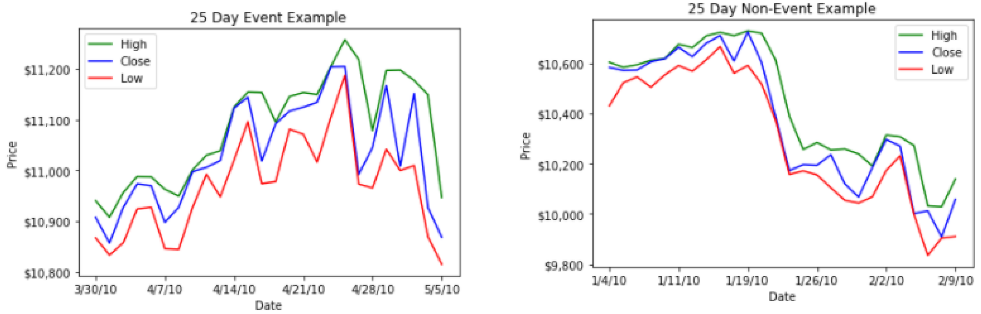
Using Figure 2 and Figure 3 below, we provide visualizations of two time series line graphs of an event and a non-event in a 25 day window along with the corresponding images we created using the steps listed above.
Our image creation process in markedly different from the work in Sezer and Ozbayoglu (2018) in which a image is generated for each day using 15 technical indicators and are labeled Buy, Hold or Sell. On the other hand, we generate an images of size that capture information from the past or 81 days, respectively, and are labeled either event or non-event.
2.3. Methods
In this subsection we describe our novel method for rare event time series classification using Siamese type neural networks. For input, we will be using the images created using the data transformation technique outlined in the previous Section 2.2. This 25 day window is often represented in a line graph like Figure 2. Figure 3 represents the corresponding image representation of those graphs.
Due to the relatively small sample size we are working with and the presence of extreme class imbalance, we chose to use a standard pre-trained CNN, namely, VGG-16 available on OpenCV (https://opencv.org, accessed on 7 November 2021). This is because the size of our dataset restricts us from effectively training our own CNN and leaves us an insufficient amount of data for testing. The pre-trained VGG-16 developed by Simonyan and Zisserman in Simonyan and Zisserman (2014) has been shown to have praise worthy results on a wide array of problems and therefore is a reasonable choice for our research.
Additionally, VGG-16 has been successfully used for transfer learning (Li et al. 2018; Liu et al. 2017). This makes VGG-16 a reasonable choice for us, since our research leverages the feature vector outputted by VGG-16 to be used to create the bootstrapped similarity distribution that is described later in this section. Furthermore, choosing a publicly available CNN like VGG-16 makes the work presented here reproducible and allows researchers to make a fair comparison across multiple datasets.
Each of the M images are passed through VGG-16. The number of images that are created is directly related to the pre-chosen size of each image. In other words, when using shorter windows of time we have more images than when longer time frames are used; the effects of the image size and count are explored in the results section.
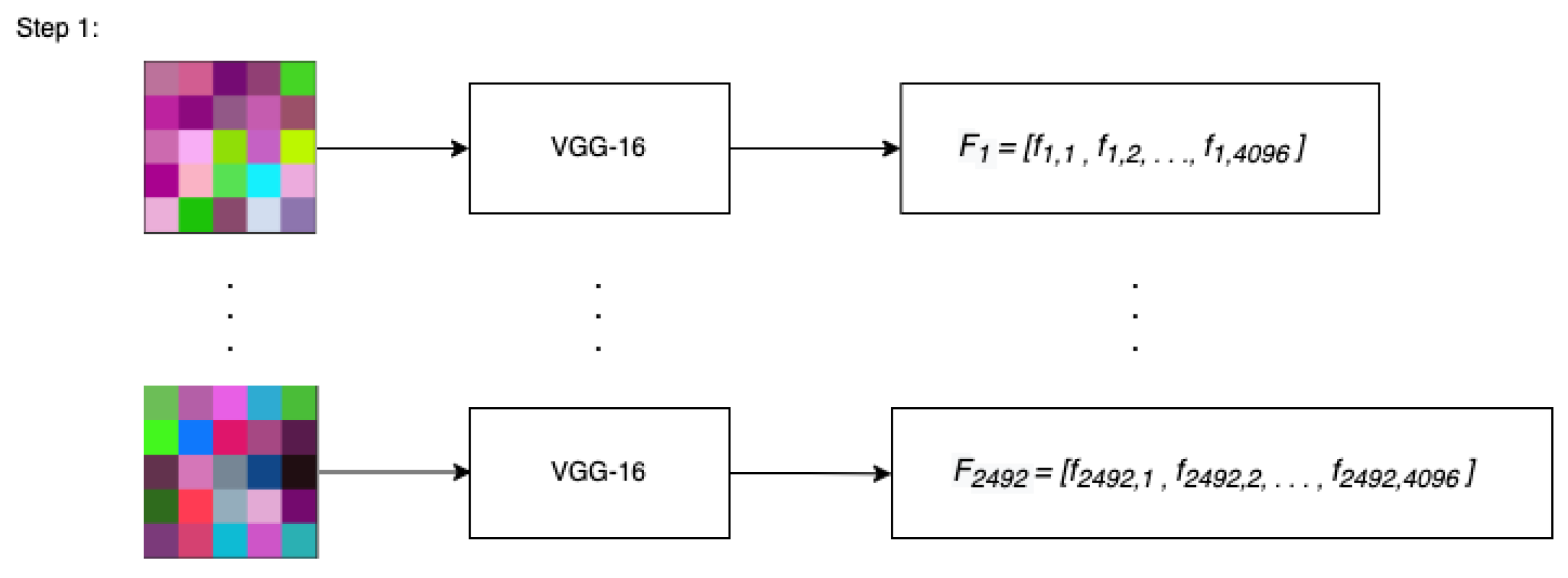
VGG-16 outputs a feature vector of size for each image passed through it. We theorize that the feature vector represents interaction effects between days that are otherwise hard to detect in methods that use tabular data. This process is repeated for all M images and the resulting feature vectors each of length 4096 are stored in a matrix. For reference we call this matrix . The size of the resulting matrix is . Each row of the matrix corresponds to the feature vector that is the output of an image. Each column of the matrix represents a specific feature of each image, extracted from the CNN. At this point the terms feature vector and image are used interchangeably. We illustrate this process in Figure 4 below.
Figure 4 shows that each of the M images are passed through the same CNN, namely VGG-16 and their output feature vector of size stored for future use. In the case of images of size , . In the figure, represents the ith row of the matrix and represents the element in the th position of .
This process can be thought of as the forward propagation of a Siamese Neural Network (SNN). Both in an SNN and in the method presented in this paper, two different images are passed through a Convolutional Neural Network with the same weights. This results in two distinct feature vectors where the Manhattan Distance is computed between them resulting in a similarity score. While other vector similarity techniques such as Euclidean distance and Cosine Similarity were experimented with, we settled with Manhattan Distance in keeping with Koch et al. (2015) which recommends using Manhattan distance for image similarity problems. Traditionally, Siamese Neural Networks are trained to maximize the similarity between same-class images and minimize the similarity between different-class images where the underlying Convolutional Neural Network’s weights are modified through backpropagation. Since we do not train this network, we consider this a Siamese-Type Neural Network as this method only uses forward propagation to yield a similarity score.
Next, we describe our bootstrapping method by first splitting the matrix into a 50/ 50 training and testing set from the median date of the time series. By splitting at the median date we ensure that there is no data leakage. In other words, by using the median date to split the matrix into training and testing, we are using the past events and non-events to predict future events. Thus, there are approximately instances in the training and testing set and each instance consists of 4096 components. This part of our methodology is in sharp contrast with the work in Sezer and Ozbayoglu (2018) in which the authors use a sliding training and testing approach on their model CNN-TA. Their process is more computationally intensive as it involves repeated re-training and testing of the model.
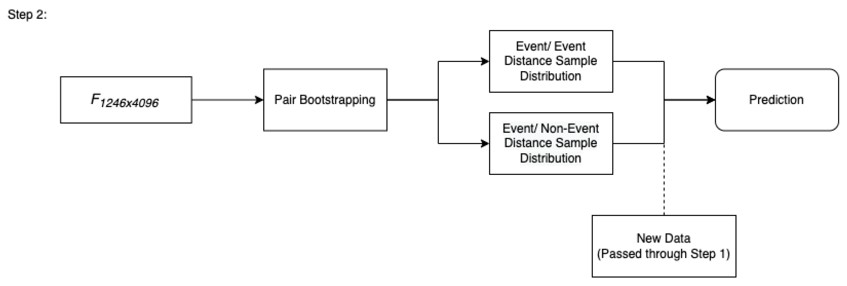
Note that purpose of the training set is not to train the CNN, since VGG-16 is a pre-trained CNN. Instead, we use the training set to create a bootstrapped distribution of similarity scores which we describe in the following sentences. Within the training set, we iteratively paired random images from the event class, computed the Manhattan Distance between each pair, and took the average of the set. The size of each set was half of the amount of the event class observations in our training data. This process was repeated until the sampled distribution of the averages of these pairs converged to an approximately normal distribution where the resulting bootstrap represents a distribution of the average similarity between pairs of event images. We refer to this as the event/event distribution. We then repeat this process but instead pair event images with non-event images This bootstrap distribution is referred to as the event/non-event distribution. We illustrate this process in Figure 5 below.
Figure 5, showcases the idea that the training set is used to create two bootstrapped distributions of the average similarity between (i) pairs of event images (referred to as the event/event distribution) and (ii) pairs of event and non-event images (referred to as event/non-event distribution). The figure also shows that the two distributions are then used to classify new images (that have been passed through step 1) as either an event or non-event.
The reason for using the bootstrapped similarity distribution is that we assume that two event feature vectors should have less distance compared to an event and non-event feature vector. By constructing bootstrapped sampling distributions of these two measures, we can then compare new data to these distributions and find the probability of a new observation belonging to either of these distributions. If the probability that this new, unknown observation belonging to the event/event distribution is higher than the event/non-event class distribution, we can classify that observation as belonging to the event class. Similarly if the opposite is found in that the probability of it belonging to the event-nonevent class distribution is higher, we classify it as a non-event. As an additional note, as this is a bootstrapped sample, these distributions are approximately normal in accordance with the Central Limit Theorem (Stine 1989).
Thus, we can compare the probabilities of a new observation belonging to a distribution using the probability density function of the normal distribution found by the mean and variance of each bootstrap. Here, the average Manhattan distance between a new observation and a set of random event class vectors are taken and the probability that this value belongs to the event/event and event/non-event distributions are calculated. The distribution that the new observation has a larger probability for belonging to is then predicted.
Formally, if x represents the average similarity score of a new image paired with random event images:
classify the new observation as an event, otherwise classify it as a non-event, where
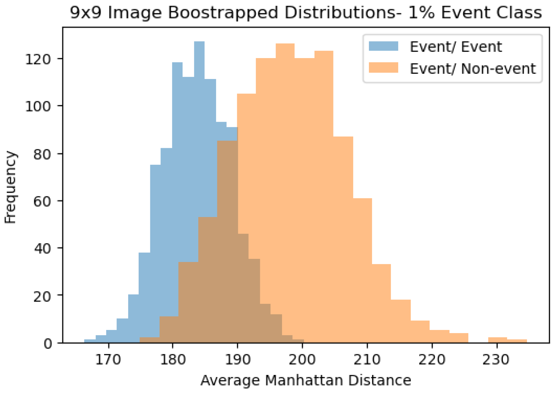
Figure 6 show the distribution of the average Manhattan distance for event/event and event/non-event images of size with a 1% class imbalance.
3. Results
We implement what was described in Section 2.2 and Section 2.3 treating the image size as a hyperparameter of our method. Here we are interested in testing the performance of our model given the financial image sizes of and . We are also interested in testing various class imbalance levels, defining the binary outcome variable we are predicting as whether an intra-day negative percent change in close price was exceeded in X% of the dataset where X is 1, 5, and 10. The performance metrics considered are: Accuracy, Precision, Recall and -Score where the results can be seen in Table 1. The total number of images on which the model was tested on across all class imbalance ratios can be found in Table 2.
Overall, our bootstrapped similarity method performed well compared to our benchmarks. While it was dependent on the size of the image and class imbalance of the dataset, we found we were able to achieve -scores of up to 14.4 percent (corresponding to images of size and class imbalance of 10%) as shown in Table 1.
4. Discussion
The research presented in this paper uses a time series of approximately 7 years resulting in 2517 instances of the S&P 500 index stocks with publicly available features: the High, Low and Close price. When converted to images of size , we end up with only about 2400 images for each case (See Table 2 for exact number of images corresponding to image size) for creating the bootstrapped distribution of average similarity scores between images and for testing. Thus, the data set being used for analysis in this paper has the following properties:
- Limited data resulting in production of limited images
- Extreme class imbalance (99-1, 95-5, 90-10) as is common with rare event prediction.
Our problem is further constrained since we use only three input features High, Low and Close price of the day. In addition to having limited data with limited features and high class imbalance, our method is restrictive based on how we chose to split the training and testing set. By choosing the median date we are guaranteeing that there is no data leakage and that future rare events are only being predicted by looking at past events and non-events. In contrast the work done by others in the field such as Buturovic and Miljkovic (2020); Sharma and Kumar (2020a) do not address the issues of limited data and high class imbalance. Furthermore, their data sets are not generated from time series.
The works of Hatami et al. (2017); Sezer and Ozbayoglu (2018); Wang and Oates (2015) use data generated from time series. However, in the case of Hatami et al. (2017); Wang and Oates (2015), the data does not arise from the financial sector and did not have the additional challenges of limited data with high class imbalance and limited input features. The work of Sezer and Ozbayoglu (2018) did use financial time series data, but their dataset is not challenged by these limitations since the goal of their paper is markedly different from our goal. In Sezer and Ozbayoglu (2018) the authors have the goal of being able to develop more profitable trading models that can predict whether one should Buy, Sell or Hold a current stock. On the other hand, our goal is to predict rare events.
In our experiments, we varied the image size and class imbalance to report the results of this novel method with different hyperparameter settings. Overall, we found that larger image sizes tended to have better classification metrics while class imbalance significantly effected model performance. We hypothesize that there are a variety of possible explanations for these findings. The first is that larger image sizes contain more information than the smaller ones which would likely result in better models. However, the largest image did not always perform the best, notably the image size outperformed the in -score for datasets with 5 and 10 percent imbalances. This could be possible due to the image spatially fitting the serial correlation in the data better than the image.
In terms of class imbalance affecting model performance, we believe this can be explained by the low number of instances of the heavily imbalanced sets. At a 1 percent event to non-event ratio, only 11 observations qualify as events in the training set. These low sample sizes may lead to non-convergence in the estimation of the true average similarity distribution between two event vectors, causing potential miss-classifications later on. Indeed, at higher event to non-event ratios, the -score tends to increase.
As a last point of discussion, a heuristic that can be used to better understand models from this method is a plot of the event/event and event/ non-event distributions. Figure 6, shows the event/event distribution in blue and the event/non-event distribution in orange, corresponding to images of size with a 1% class imbalance. Ideally, the two distributions would be well separated along the x-axis. A small intersection would suggest that the two distributions are well separated and thus new comparisons of similarity would thus be classified with a higher confidence to a particular distribution.
Benchmark models used included Logistic Regression, and a variety of other standard binary classification methods such as Random Forest, XGBoost, K-Nearest Neighbor and Naive Bayes. The feature vector extracted from the CNN: VGG-16 was used as input for these baseline models. In an attempt to boost the performance of benchmark models several techniques were employed. For instance,
- image size, class imbalance level and training and testing split ratios were varied
- Principal Component Analysis (PCA) on the matrix before training and testing was performed
- different types of re-sampling techniques were used and
- hyperparameter variations were considered.
We found that the actions listed above yielded benchmark models unable to make event predictions. Specifically, our benchmark models resulted in having high accuracy, but 0 percent -scores as they only made predictions for non-events. This is consistent with existing literature (Johnson and Khoshgoftaar 2019). In comparison, we found that our method of using a bootstrapped distribution of similarity scores outperformed traditional binary classification approaches to the problem of identifying rare events in financial time series because our -scores were all greater than 0.
We also investigated the explanatory power of the feature vectors extracted from the CNNs by using them as predictors in time series classification models in comparison to training classification models on traditional High, Low, Close variables only. Models with the feature vectors were generally found favorable over models just using HLC variables, although further research needs to be done to assess this potential gain in a more systematic way and on multiple different time series data sets.
5. Conclusions
In this paper the S&P 500 index was examined using a novel method that consisted of (i) converting tabular data into images (ii) passing the resulting images in a CNN and (iii) examining similarity scores using the output vector of size with the intention of being able to identify rare events. All baseline models explored failed to predict an image as an event. For instance, the Logistic Regression model yielded an -score of 0, whereas our proposed method was able to achieve -scores of up to percent.
Thus, the work presented in this paper attempts to tackle a notoriously difficult problem of predicting rare events in financial markets with limited features and limited observations. Our results indicate even with these shortcomings, this method has the ability to identify patterns correlated with events better than baselines and in a context ill suited for other methods proposed in the literature.
While the results of this paper are comparable to other research outcomes in the field of stock market event prediction (Shen et al. 2012; Tsai and Wang 2009), the focus of our research is to present a new concept of implementing time series features through image representation and Siamese type neural networks. Using the methodology developed in this paper we were able to show that our approach results in significant improvement on time series event classification. Additionally, while this paper can be considered as introduction of a new framework of how to represent data for time series forecasting, we are certain that future research will be able to further improve performance and methodology.
There are multiple ways in which our work may be extended.
- The first is that an active learning approach (Malialis et al. 2020) can be applied to this method in which after every day, the two bootstraps are retaken to include the new observation. While this method may be computationally expensive, it could lead to a more pronounced separation in the event/event and event/non-event distributions, thereby leading to better predictions.
- In this paper we proposed a “snake" method to transform time series into images. Since there a variety of ways to visualize tabular data as an image (Hatami et al. 2017; Sezer and Ozbayoglu 2018; Sharma et al. 2019; Sharma and Kumar 2020a; Sun et al. 2019), we note this as a means to parameterize or tune our method for other future applications. For instance, the research presented in this paper made use of square images. However, one could consider circular images (Wang and Oates 2015), textured images (Sharma and Kumar 2020b) or images created through Markov Transition Field (MTF) (Wang and Oates 2015). Further research can be done to compare image shape or similarly develop new transformation techniques that result in other types of images.
- We believe different image classification frameworks such as ResNet50 (https://arxiv.org/abs/1512.03385, accessed on 7 November 2021) can be experimented with to further improve results as they can effect the image resizing as well as the output feature vector that is used for similarity comparisons.
- For this research we used time series data from only the S&P 500 index. The combination of S&P 500 with other time series data such as Dow Jones (https://finance.yahoo.com/quote/%5EDJI/, accessed on 7 November 2021) or Nasdaq (https://finance.yahoo.com/quote/%5EIXIC/, accessed on 7 November 2021) could help to identify further patterns to improve prediction accuracy, or related derived metrics such as volatility indexes.
- Lastly, although this paper investigated daily financial time series data (HLC) to predict and identify patterns for rare event prediction, the proposed approach could also be applied to intra-day trading applications as technical analyses are even more relevant there.
Author Contributions
Conceptualization, T.B. and I.S.; Methodology, T.B., O.M., I.S. and J.W.; Software, O.M. and J.W.; Validation, T.B., O.M., I.S. and J.W.; Formal analysis, T.B., O.M., I.S. and J.W.; Investigation, T.B., O.M., I.S. and J.W.; Data Curation, J.W.; Writing—T.B., O.M., I.S., J.W.; Writing—review and editing, T.B., O.M., I.S., J.W.; Visualization, J.W. All authors have read and agreed to the published version of the manuscript.
Funding
This research received no external funding.
Data Availability Statement
Our data can be found at: Yahoo Finance (accessed on 1 November 2021).
Acknowledgments
The authors would also like to thank Michael Proksch for his insightful thoughts on the manuscript. We gratefully acknowledge the reviewers of Risks for their helpful comments and suggestions which improved the quality of this work.
Conflicts of Interest
The authors declare no conflict of interest.
References
- Ali, Ozden Gur, and Umut Ariturk. 2014. Dynamic churn prediction framework with more effective use of rare event data: The case of private banking. Expert Systems with Applications 17: 7889–903. [Google Scholar]
- Bettman, Jenni L., Stephen J. Sault, and Emma L. Schultz. 2009. Fundamental and technical analysis: Substitutes or complements? Accounting & Finance 49: 21–36. [Google Scholar]
- Barndorff-Nielsen, Ole E., and Neil Shephard. 2001a. Non-Gaussian Ornstein-Uhlenbeck-based models and some of their uses in financial economics. Journal of the Royal Statistical Society Series B (Statistical Methodology) 63: 167–241. [Google Scholar] [CrossRef]
- Barndorff-Nielsen, Ole E., and Neil Shephard. 2001b. Modelling by Lévy processes for financial econometrics. In Lévy Processes: Theory and Applications. Edited by Ole E. Barndorff-Nielsen, Thomas Mikosch and Sidney I. Resnick. Basel: Birkhäuser, pp. 283–318. [Google Scholar]
- Buturovic, Ljubomir, and Dejan Miljkovic. 2020. A novel method for classification of tabular data using convolutional neural networks. bioRxiv. [Google Scholar] [CrossRef]
- Chavarnakul, Thira, and David Enke. 2008. Intelligent technical analysis based equivolume charting for stock trading using neural networks. Expert Systems with Applications 34: 1004–17. [Google Scholar] [CrossRef]
- Cheng, Ching-Hsue, and You-Shyang Chen. 2007. Fundamental Analysis of Stock Trading Systems using Classification Techniques. Paper presented at International Conference on Machine Learning and Cybernetics, Hong Kong, China, August 19–22; pp. 1377–82. [Google Scholar] [CrossRef]
- Cheon, Seong-Pyo, Sungshin Kim, So-Young Lee, and Chong-Bum Lee. 2009. Bayesian networks based rare event prediction with sensor data. Knowledge-Based Systems 22: 336–43. [Google Scholar] [CrossRef]
- Drakopoulou, Veliota. 2016. A Review of Fundamental and Technical Stock Analysis Techniques. Journal of Stock Forex Trading 5. [Google Scholar] [CrossRef]
- Ekapure, Shubham, Nuruddin Jiruwala, Sohan Patnaik, and Indranil SenGupta. 2021. A data-science-driven short-term analysis of Amazon, Apple, Google, and Microsoft stocks. arXiv arXiv:2107.14695. [Google Scholar]
- Esteva, Andre, Brett Kuprel, Roberto A. Novoa, Justin Ko, Susan M. Swetter, Helen M. Blau, and Sebastian Thrun. 2017. Dermatologist-level classification of skin cancer with deep neural networks. Nature 542: 115–18. [Google Scholar] [CrossRef]
- Gumbel, Emil Julius. 1958. Statistics of Extremes. New York: Columbia University Press. [Google Scholar]
- Habtemicael, Semere, and Indranil SenGupta. 2016. Pricing variance and volatility swaps for Barndorff-Nielsen and Shephard process driven financial markets. International Journal of Financial Engineering 3: 165002. [Google Scholar] [CrossRef]
- Hatami, Nima, Yann Gavet, and Johan Debayle. 2017. Classification of time series images using deep convolutional neural networks. Paper presented at International Conference on Machine Vision, Tenth International Conference on Machine Vision (ICMV), Vienna, Austria, November 13–15. [Google Scholar]
- Hu, Zexin, Yiqi Zhao, and Matloob Khushi. 2021. A Survey of Forex and Stock Price Prediction Using Deep Learning. Applied System Innovation 4: 9. [Google Scholar] [CrossRef]
- Issaka, Aziz, and Indranil SenGupta. 2017. Analysis of variance based instruments for Ornstein-Uhlenbeck type models: Swap and price index. Annals of Finance 13: 401–34. [Google Scholar] [CrossRef]
- Janjuaa, Zaffar Haider, Massimo Vecchioa, Mattia Antonini, and Fabio Antonelli. 2019. Antoniniab. Antonelli IRESE: An intelligent rare-event detection system using unsupervised learning on the IoT edge. Engineering Applications of Artificial Intelligence 84: 41–50. [Google Scholar] [CrossRef] [Green Version]
- Johnson, Justin M., and Taghi M. Khoshgoftaar. 2019. Survey on deep learning with class imbalance. Journal of Big Data 6. [Google Scholar] [CrossRef]
- Koch, Gregory, Richard Zemel, and Ruslan Salakhutdinov. 2015. Siamese neural networks for one- shot image recognition. Presented at the Deep Learning Workshop at the 2015 International Conference on Machine Learning, Lille, France; Available online: https://www.cs.cmu.edu/~rsalakhu/papers/oneshot1.pdf (accessed on 1 November 2021).
- Li, Jinyan, Lian-sheng Liu, Simon Fong, Raymond K. Wong, Sabah Mohammed, Jinan Fiaidhi, Yunsick Sung, and Kelvin K. L. Wong. 2017. Adaptive swarm balancing algorithms for rare-event prediction in imbalanced healthcare data. PLoS ONE 12: e0180830. [Google Scholar] [CrossRef] [Green Version]
- Li, Xuhong, Yves Grandvalet, and Franck Davoine. 2018. Explicit inductive bias for transfer learning with convolutional networks. Paper presented at International Conference on Machine Learning, Stockholm, Sweden, July 10–15; pp. 2825–34. [Google Scholar]
- Lin, Minglian, and Indranil SenGupta. 2021. Analysis of optimal portfolio on finite and small time horizons for a stochastic volatility market model. SIAM Journal on Financial Mathematics 12: 1596–624. [Google Scholar] [CrossRef]
- Liu, Jiaming, Yali Wang, and Yu Qiao. 2017. Sparse deep transfer learning for convolutional neural network. Paper presented at Thirty-First AAAI Conference on Artificial Intelligence, San Francisco, CA, USA, February 4–9. [Google Scholar]
- Malialis, kleanthis, Christos G. Panayiotou, and Marios M. Polycarpou. 2020. Data-efficient Online Classification with Siamese Networks and Active Learning. Paper presented at International Joint Conference on Neural Networks (IJCNN 2020), Glasgow, UK, July 19–24. [Google Scholar]
- Murphy, John J. 1999. Technical Analysis of the Financial Markets: A Comprehensive Guide to Trading Methods and Applications. New York: New York Institute of Finance. [Google Scholar]
- Nazário, Rodolfo Toríbio Farias, Lima e Silva, Jéssica, Vinicius Amorim Sobreiro, and Herbert Kimura. 2017. A literature review of technical analysis on stock markets. The Quality Review of Economics and Finance 66: 115–26. [Google Scholar]
- Rao, Vishwas, Romit Maulik, Emil Constantinescu, and Mihai Anitescu. 2020. A Machine-Learning-Based Importance Sampling Method to Compute Rare Event Probabilities. In Computational Science-ICCS. Lecture Notes in Computer Science. Cham: Springer, volume 12142. [Google Scholar]
- Roberts, Michael, and Indranil SenGupta. 2020. Sequential hypothesis testing in machine learning, and crude oil price jump size detection. Applied Mathematical Finance 27: 374–95. [Google Scholar] [CrossRef]
- Salmon, Nicholas, and Indranil SenGupta. 2021. Fractional Barndorff-Nielsen and Shephard model: Applications in variance and volatility swaps, and hedging, Annals of Finance. Annals of Finance 17: 529–558. [Google Scholar] [CrossRef]
- SenGupta, Indranil. 2016. Generalized BN-S stochastic volatility model for option pricing. International Journal of Theoretical and Applied Finance 19: 1650014. [Google Scholar] [CrossRef]
- SenGupta, Indranil, William Nganje, and Erik Hanson. 2021. Refinements of Barndorff-Nielsen and Shephard model: An analysis of crude oil price with machine learning. Annals of Data Science 8: 39–55. [Google Scholar] [CrossRef] [Green Version]
- Sezer, Omer Berat, and Ahmet Murat Ozbayoglu. 2018. Algorithmic financial trading with deep convolutional neural networks: Time series to image conversion approach. Applied Soft Computing 70: 525–538. [Google Scholar] [CrossRef]
- Sharma, Alok, Edwin Vans, Daichi Shigemizu, Keith A. Boroevich, and Tatsuhiko Tsunoda. 2019. DeepInsight: A methodology to transform a non-image data to an image for convolution neural network architecture. Scientific Reports 9: 1–7. [Google Scholar] [CrossRef] [PubMed] [Green Version]
- Sharma, Anuraganand, and Dinesh Kumar. 2020a. Classification with 2-D Convolutional Neural Networks for breast cancer diagnosis. arXiv arXiv:2007.03218v2. [Google Scholar]
- Sharma, Anuraganand, and Dinesh Kumar. 2020b. Non-image data classification with convolutional neural networks. arXiv arXiv:2007.03218. [Google Scholar]
- Shen, Shunrong, Haomiao Jiang, and Tongda Zhang. 2012. Stock Market Forecasting Using Machine Learning Algorithms. Stanford: Department of Electrical Engineering, Stanford University, pp. 1–5. [Google Scholar]
- Shoshi, Humayra, and Indranil SenGupta. 2021. Hedging and machine learning driven crude oil data analysis using a refined BarndorffNielsen and Shephard model. International Journal of Financial Engineering 8: 2150015. [Google Scholar] [CrossRef]
- Simonyan, Karen, and Andrew Zisserman. 2014. Very Deep Convolutional Networks for Large-Scale Image Recognition. arXiv arXiv:1409.1556. [Google Scholar]
- Stine, Robert. 1989. An Introduction to Bootstrap Methods: Examples and Ideas. Sociological Methods & Research 18: 243–91. [Google Scholar]
- Sun, Baohua, Lin Yang, Wenhan Zhang, Michael Lin, Patrick Dong, Charles Young, and Jason Dong. 2019. Supertml: Two-dimensional word embedding for the precognition on structured tabular data. Paper presented at IEEE Conference on Computer Vision and Pattern Recognition Workshops, Nashville, TN, USA, June 19–25. [Google Scholar]
- Taigman, Yaniv, Ming Yang, Marc’Aurelio Ranzato, and Lior Wolf. 2014. DeepFace: Closing the Gap to Human-Level Performance in Face Verification. Paper presented at the IEEE Conference on Computer Vision and Pattern Recognition (CVPR), Columbus, OH, USA, June 23–28; pp. 1701–8. [Google Scholar]
- Tsai, Chih-Fong, and S. P. Wang. 2009. Stock Price Forecasting by Hybrid Machine Learning Techniques. Paper presented at International MultiConference of Engineers and Computer Scientists, Hong Kong, China, March 18–20. [Google Scholar]
- Vijh, Mehar, Deeksha Chandola, Vinay Anand Tikkiwal, and Arun Kumar. 2020. Stock Closing Price Prediction using Machine Learning Techniques. Procedia Computer Science 167: 599–606. [Google Scholar] [CrossRef]
- Wang, Zhiguang, and Tim Oates. 2015. Imaging time series to improve classification and imputation. Paper presented at 24th International Conference on Artificial Intelligence, Buenos Aires, Argentina, July 25–31; pp. 3939–45. [Google Scholar]
- Weiss, Gary M., and Haym Hirsh. 2000. Learning to Predict Extremely Rare Events. Technical Report WS-00-05. Paper presented at Learning from Imbalanced Data Sets, AAAI Workshop, Menlo Park, CA, USA, July 31; pp. 64–68. [Google Scholar]
Figure 1.
Sample image representing a 25 day period with HLC as input.

Figure 2.
Examples of line graphs that show 25 days leading up to an event and non-event.

Figure 3.
Corresponding image reconstructions of the time series in Figure 2.
Figure 3.
Corresponding image reconstructions of the time series in Figure 2.

Figure 4.
Images of size passed through VGG-16 resulting in .

Figure 5.
Diagram illustrating the process by which new predictions are made.

Figure 6.
9 × 9 Image Bootstrapped Distributions.


Table 1.
Comparing performance metrics in the test data set across all image sizes and class imbalance ratios.
Table 1.
Comparing performance metrics in the test data set across all image sizes and class imbalance ratios.
| Image Size | Class Imbalance | Accuracy | Precision | Recall | Score |
|---|---|---|---|---|---|
| 5 × 5 | 1% | 0.691 | 0.010 | 0.364 | 0.020 |
| 5% | 0.763 | 0.024 | 0.105 | 0.039 | |
| 10% | 0.819 | 0.086 | 0.109 | 0.096 | |
| 6 × 6 | 1% | 0.687 | 0.005 | 0.182 | 0.010 |
| 5% | 0.776 | 0.041 | 0.179 | 0.067 | |
| 10% | 0.808 | 0.083 | 0.121 | 0.098 | |
| 7 × 7 | 1% | 0.580 | 0.008 | 0.364 | 0.015 |
| 5% | 0.795 | 0.067 | 0.259 | 0.106 | |
| 10% | 0.826 | 0.131 | 0.159 | 0.144 | |
| 8 × 8 | 1% | 0.678 | 0.008 | 0.273 | 0.015 |
| 5% | 0.708 | 0.048 | 0.267 | 0.082 | |
| 10% | 0.707 | 0.086 | 0.239 | 0.127 | |
| 9 × 9 | 1% | 0.765 | 0.011 | 0.273 | 0.021 |
| 5% | 0.782 | 0.044 | 0.167 | 0.070 | |
| 10% | 0.835 | 0.123 | 0.138 | 0.130 |
Table 2.
Number of test images of each size across all class imbalance.
| Image Size | Imbalance | Event Images | Non-Event Images | Total |
|---|---|---|---|---|
| 1% | 11 | 1235 | 1246 | |
| 5% | 57 | 1189 | ||
| 10% | 110 | 1136 | ||
| 1% | 11 | 1230 | 1241 | |
| 5% | 56 | 1185 | ||
| 10% | 107 | 1134 | ||
| 1% | 11 | 1216 | 1227 | |
| 5% | 58 | 1169 | ||
| 10% | 113 | 1114 | ||
| 1% | 11 | 1216 | 1227 | |
| 5% | 60 | 1167 | ||
| 10% | 109 | 1118 | ||
| 1% | 11 | 1207 | 1219 | |
| 5% | 60 | 1158 | ||
| 10% | 109 | 1110 |
Publisher’s Note: MDPI stays neutral with regard to jurisdictional claims in published maps and institutional affiliations. |
© 2022 by the authors. Licensee MDPI, Basel, Switzerland. This article is an open access article distributed under the terms and conditions of the Creative Commons Attribution (CC BY) license (https://creativecommons.org/licenses/by/4.0/).
Share and Cite
MDPI and ACS Style
Basu, T.; Menzer, O.; Ward, J.; SenGupta, I. A Novel Implementation of Siamese Type Neural Networks in Predicting Rare Fluctuations in Financial Time Series. Risks 2022, 10, 39. https://0-doi-org.brum.beds.ac.uk/10.3390/risks10020039
AMA Style
Basu T, Menzer O, Ward J, SenGupta I. A Novel Implementation of Siamese Type Neural Networks in Predicting Rare Fluctuations in Financial Time Series. Risks. 2022; 10(2):39. https://0-doi-org.brum.beds.ac.uk/10.3390/risks10020039
Chicago/Turabian StyleBasu, Treena, Olaf Menzer, Joshua Ward, and Indranil SenGupta. 2022. "A Novel Implementation of Siamese Type Neural Networks in Predicting Rare Fluctuations in Financial Time Series" Risks 10, no. 2: 39. https://0-doi-org.brum.beds.ac.uk/10.3390/risks10020039
Note that from the first issue of 2016, this journal uses article numbers instead of page numbers. See further details here.