Recent Regulation in Credit Risk Management: A Statistical Framework

Abstract

A recently introduced accounting standard, namely the International Financial Reporting Standard 9, requires banks to build provisions based on forward-looking expected loss models. When there is a significant increase in credit risk of a loan, additional provisions must be charged to the income statement. Banks need to set for each loan a threshold defining what such a significant increase in credit risk constitutes. A low threshold allows banks to recognize credit risk early, but leads to income volatility. We introduce a statistical framework to model this trade-off between early recognition of credit risk and avoidance of excessive income volatility. We analyze the resulting optimization problem for different models, relate it to the banking stress test of the European Union, and illustrate it using default data by Standard and Poor’s.

1. Introduction

The global financial crisis of 2007–2008 highlighted the delayed recognition of credit losses as a weakness of the accounting standards at that time. As a result, the International Accounting Standards Board introduced International Financial Reporting Standard (IFRS) 9, which is an accounting standard that requires banks to recognize increased credit risk of loans early and build additional provisions for such loans. Because loss provisions affect banks’ income statements, it is critical to have accurate estimations of these values for each reporting period. However, the building of provisions and their subsequent release for reduced credit risk leads to undesired volatility in the income statements of banks. In this paper, we introduce and analyze a framework to model this trade-off between early recognition of increased credit risk and avoidance of excessive income volatility.

IFRS 9, being mandatory since 1 January 2018, requires banks to consider forward-looking expected loss impairment models. Randall and Thompson (2017) outlined that forward-looking information regarding credit risk includes qualitative information, such as the current economic environment, along with both statistical models and non-statistical quantitative information. On the contrary, the previously used backward-looking approach required a trigger event to occur prior to any credit losses being reported. Qualitative information to complement methods from statistics and operational research has been used in credit risk modelling beyond applications related to IFRS 9; see Angilella and Mazzù (2017); Crook et al. (2007); Kumar and Ravi (2007). Regardless of the specific information considered, there is still a subjective aspect involved in a financial institution’s assessment of credit risk for loans, but it is crucial for each bank to have a sound underlying modelling framework.

Under IFRS 9, banks are required to estimate the expected credit loss (ECL) for each loan and build corresponding provisions. Compared to charging only highly likely or even realized credit losses, this procedure allows for early recognition of credit risk, well before an actual default occurs. The new standards require various ECL measures for loans classified into three different buckets of progressively higher default risk, compared to the initial default risk when the loan is issued; see Cohen and Edwards (2017); Maggi et al. (2017). To avoid misunderstandings, these IFRS 9 buckets are not to be confused with the typical rating buckets in which banks group obligors with similar credit ratings, within their diversified loan portfolio.

Table 1. ECL calculation criteria for loans, relative to their IFRS 9 classification.

IFRS 9	Loan Type	ECL
bucket 1	performing	one-year
bucket 2	underperforming	lifetime
bucket 3	impaired	lifetime

provides a summary of the structure of the IFRS 9 buckets. ECL is estimated over a one-year period for loans in bucket 1, when the obligor generally possesses “good credit” relative to their initial credit quality, so it is considered to be a performing loan in this case.

The reclassification of a loan takes place when deteriorating credit quality of an obligor is observed, based on predefined warning signs. These warning signs involve an increased probability of default, in accordance with the current forecast of the credit environment. Therefore, IFRS 9 bucket 2 represents underperforming loans that have experienced a significant increase in credit risk since initial recognition. Furthermore, impaired loans, which result in the bank actually incurring credit losses, are classified in bucket 3.

An important feature of this classification is that, for underperforming loans (bucket 2), lifetime ECL is estimated over the remaining term to maturity, rather than one-year ECL. Clearly, the ECL of a loan in bucket 2, especially in the early stages of the period of the loan, would typically be much greater than the ECL of a loan in bucket 1. It must be noted that, for loans in bucket 3, ECL is estimated based on the bank’s exposure along with the estimated recovery values. The subjective nature of this IFRS 9 classification is critical when analyzing, from the perspective of a financial institution, what a significant increase in credit risk actually is, as this is not specified in IFRS 9.

It is quite challenging to decide on the threshold for precisely defining a significant increase in credit risk, for numerous reasons. If an extremely conservative framework is implemented by a bank, its obligors would only need to experience minor indicators of credit downturn to warrant a reclassification from bucket 1 to bucket 2. In this instance, the bank’s ECL calculations are prone to volatility, as loans could transfer from one-year ECL to lifetime ECL frequently. However, setting a threshold that is very lenient towards obligor’s credit quality would indeed create more stable ECL calculations for the bank, but at the same time lead to late recognition of credit risk with respect to these loans. Finding a balance between early recognition of credit risk and income volatility, in this sense, is an interesting problem that is at the heart of this paper and directly linked to the new loss impairment standards of IFRS 9. Indeed, a survey by the European Banking Authority (2017) found that “72% of the banks included in the survey anticipate that IFRS 9 impairment requirements will increase volatility in profit or loss…mainly due to the “cliff effect” when moving exposures from stage 1 to stage 2 (from 12-month ECL to lifetime ECL)…”

Our setting is based on the structural model of default by Merton (1974). It essentially states that an obligor can only meet its financial obligations if the value of their assets exceeds that of the liabilities at the time of maturity, for a single debt obligation. While the actual nature of an individual obligor’s debt is considerably more complex, with default possible at several times, the preceding assumptions do provide us with a quality, widely used starting point for credit risk modelling. There have been extensions in terms of asset value modelling (see Bluhm et al. (2010); Bohn and Stein (2009); McNeil et al. (2015) for an overview), but the Merton model remains the “prototype” of many credit risk models, such as Bluhm and Overbeck (2003); Frei and Wunsch (2018); Gordy (2000). In particular, the Merton model is at the basis of the capital requirement described by the Basel Committee on Banking Supervision (2005), whose framework Miu and Ozdemir (2017) suggest to employ for IFRS 9 purposes. Such models have also been applied for stress testing; see, for example, Miu and Ozdemir (2009); Simons and Rolwes (2009); Yang and Du (2015).

Since Merton (1974) models the underlying asset value of the obligor as a stochastic process over time, we can formulate an optimization problem that considers the impact on the income statement at different reporting moments. The optimization problem consists of two penalization terms: (1) a term to penalize for failing to early recognize an eventual default, and (2) a term that penalizes for income volatility. We weight the two terms by a tuning parameter, which determines the relative importance of low income volatility compared to early credit recognition. While IFRS 9 does not define exactly what a significant increase in credit risk is, and thus leaves flexibility in choosing our tuning parameter, we apply the stress test framework of the European Banking Authority (2018) to obtain a suitable estimation for this parameter. The optimization problem is involved, but we solve it analytically for certain distributions of the asset value process. For the classical setting of Merton (1974), where the asset value process is modelled as a Brownian motion, we recast it as an optimization problem that we solve efficiently by numerical routines and illustrate using default data from Standard and Poor’s (2018).

The introduction of IFRS 9 has implications on credit risk measurement and management, which go far beyond the question of building suitable provisions for ECL. In terms of a bank’s risk appetite framework, which assesses and determines the level of risk the bank is prepared to accept (see Stulz (2015)), banks need to take effects of ECL provision building and particularly its ramifications on income volatility into account. Thus, not only the default probability of an obligor at a given moment in time matters, but it also becomes crucial how volatile and sensitive the obligor’s credit risk is to changes in the economic environment. Our proposed framework models both of these aspects and allows for a quantification of the associated risk. As a consequence of IFRS 9, banks will adjust their product offerings and business strategies, for example, by reducing lending to clients and sectors that may be too risky or volatile under IFRS 9.

As required by IFRS 9, we compute credit provisions in a forward-looking way. Such forward-looking models are related to scenario analysis; see Miu and Ozdemir (2017); Skoglund and Chen (2016). The building of provisions for ECL under IFRS 9 also has important implications on banks’ capital assessments: Principle 11 of the Basel Committee on Banking Supervision (2015) requires banking supervisors to consider banks’ credit risk practices and recognize their ECL processes and models when assessing capital adequacy. Moreover, IFRS 9 incentivizes banks to reform their credit management polices and provide additional training to their relationship managers, so that they can help reduce the risk of credit deterioration and propose mitigation actions to prevent loans from becoming underperforming and falling into bucket 2; compare also Maggi et al. (2017).

The remainder of this paper is organized as follows. Section 2 introduces a credit risk model that captures the trade-off between early recognition of credit risk and income volatility. The resulting optimization problem is analyzed when the latent asset return has either a continuous distribution (Section 3) or discrete distribution (Section 4). In Section 5, we compare our model with the stress test framework of the European Banking Authority (2018) and apply it to default data from Standard and Poor’s (2018). Section 6 provides the conclusions.

2. Modelling Income Volatility and Early Recognition of Credit Risk

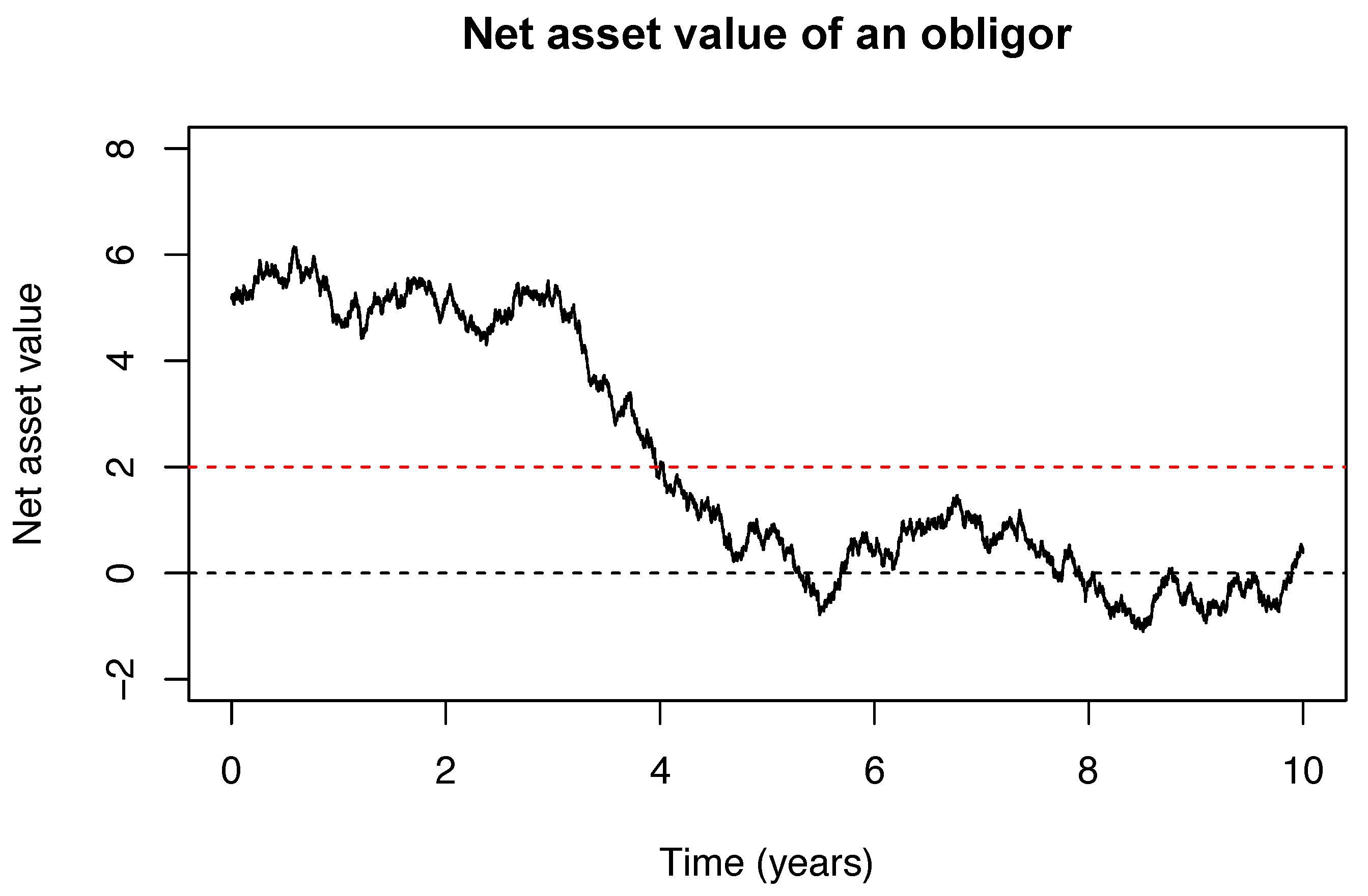
When considering an obligor being issued a loan from a bank, we can model the trade-off between income volatility and the early recognition of credit risk. The net asset value of the obligor at time $t\in [0,T]$ can be represented by $A_t$ for a stochastic process ${(A_t)}_{0\le t\le T}$, akin to the Merton model’s basic framework. In contrast to the Merton model, we do not impose that ${(A_t)}_{0\le t\le T}$ is a Brownian motion, but only assume that this stochastic process has stationary and independent increments. We measure time t in years. The starting point $A_0=k$ is the initial distance to default of an obligor, based on their initial default probability. We then let c denote the threshold in which the obligor’s credit quality drops from bucket 1 to bucket 2 in terms of the IFRS 9 classification, for some constants $c\in [0,k]$. Figure 1 provides an example of the net asset value of an obligor with a loan over $T=10$ years. To explain further, if $A_t>c$, the obligor’s loan is in bucket 1, signifying “good credit” relative to their initial credit quality at the time the loan was issued. We define that a default at time T occurs if $A_T<0$, and, consequently, the initial distance to default of the obligor is equal to k. Furthermore, when $A_t\le c$, the loan is in bucket 2, which means the bank’s provisions for this obligor’s particular loan are calculated based on lifetime expected credit loss rather than one-year expected credit loss. We assume that there needs to be enough assets to pay back the loan only at the maturity time T, so that we consider default events only at T, consistent with the modelling of default in the Merton model. Hence, in Figure 1, although the obligor’s loan experiences a significant increase in credit risk at approximately $T=4$, a default does not occur, since its asset value evidently exceeds that of its liabilities at maturity, $T=10$.

To establish an optimization problem, a formulation involving discrete-time observations is incorporated. This logic is quite realistic, as obligor specific information from a bank is typically observed at monthly or quarterly reporting dates. Here, we consider instances $t_0=0<t_1<\cdots <t_N=T$ and assume that $t_{N-1}\le T-1$. This assumption is without loss of generality, as we could simply disregard the instances after reporting time $T-1$. There is no impact on provisions when switching above and below the threshold c after $T-1$, as one-year ECL equals lifetime ECL during the final year of the loan. Prior to formally defining the actual optimization problem, we examine the two portions of the prospective objective function, which will model the trade-off between income volatility and the early recognition of credit risk. The recognition portion is

$$\sum _{j=1}^{N-1}(T-1-t_j)P(A_{t_j}>c|A_T<0),$$

(1)

while the volatility portion is

$$E\left[\sum _{j=1}^{N-1}(T-1-t_j){\left({11}_{A_{t_j}>c}-{11}_{A_{t_{j-1}}>c}\right)}^2\right].$$

(2)

As we subsequently explain in more detail, the recognition portion penalizes for failing to early recognize a default while the volatility portion measures fluctuations resulting from reclassifications between buckets 1 and 2. We first examine the probability, $P(A_{t_j}>c|A_T<0)$, which is part of Formula (1), representing the conditional probability that the net asset value of the obligor at time $t_j$ exceeds c, given a default occurs at time T. Hence, if this probability is low, the early recognition of credit risk is likely, since experiencing the “warning sign” of a loan being classified in bucket 2 before a default occurs is probable. Intuitively, this probability being low would correspond to a high threshold value c, near $A_0=k$. In Formula (2), the expression ${\left({11}_{A_{t_j}>c}-{11}_{A_{t_{j-1}}>c}\right)}^2$ gives the value 1 (and zero otherwise) if the process changes from being above to below (or vice versa) the threshold c from time $t_{j-1}$ to $t_j$. As we would expect, if c is high, the net asset value of an obligor is more prone to fluctuation between classification buckets 1 and 2. This would lead to frequent adjustments in the calculation of ECL, changing from one-year ECL to lifetime ECL, and vice versa, ultimately contributing to substantial earnings volatility from the perspective of the bank that issues the loan. We recall here that ECL equals the product of probability of default (PD), loss given default (LGD), and exposure at default (EaD). In practice, LGD and EaD are often assumed to be constant so that the PD, which we capture in this term, models the default risk. The summations in both Formulae (1) and (2) capture the net asset value throughout each time step, up until the final year of the loan. The coefficient $(T-1-t_j)$ in both portions conveys that the early recognition of credit risk, along with the management of income volatility, is more critical earlier in the term of the loan. Thus, each portion has a negative, approximately linear relationship with time. First of all, the earlier the risk of non-payment is identified, the sooner loan loss provisions can be built proactively. Relative to income volatility, the earlier a significant increase in credit risk occurs, the larger the impact on a bank’s income relative to ECL estimation, hence the factor $(T-1-t_j)$. We can write the volatility portion (2) as

$$\begin{array}{c}E\left[\sum _{j=1}^{N-1}(T-1-t_j){\left({11}_{A_{t_j}>c}-{11}_{A_{t_{j-1}}>c}\right)}^2\right]\hfill \\ =\sum _{j=1}^{N-1}(T-1-t_j)\left(P\left(A_{t_j}>c,A_{t_{j-1}}\le c\right)+P\left(A_{t_j}\le c,A_{t_{j-1}}>c\right)\right),\hfill \end{array}$$

using ${\left({11}_{A_{t_j}>c}-{11}_{A_{t_{j-1}}>c}\right)}^2={11}_{A_{t_j}>c,A_{t_{j-1}}\le c}+{11}_{A_{t_j}\le c,A_{t_{j-1}}>c}$.

Acknowledging that Formulae (1) and (2) are decreasing and increasing in c, respectively, we combine these two portions and model the inherent balance between early recognition of credit risk and income volatility through the optimization problem

$$\underset{c\le k}{min}f(c),$$

where

$$\begin{array}{cc}\hfill f(c)=& \sum _{j=1}^{N-1}(T-1-t_j)P(A_{t_j}>c|A_T<0)\hfill \\ & +\lambda \sum _{j=1}^{N-1}(T-1-t_j)\left(P\left(A_{t_j}>c,A_{t_{j-1}}\le c\right)+P\left(A_{t_j}\le c,A_{t_{j-1}}>c\right)\right).\hfill \end{array}$$

(3)

Note that $\lambda >0$ is a tuning parameter that, in practical terms, determines how much importance is placed on minimizing income volatility from the perspective of a bank. Various approaches to modelling the net asset value process ${(A_t)}_{0\le t\le T}$ will be investigated in the following sections, including both continuous and discrete distributions for the increments of ${(A_t)}_{0\le t\le T}$.

3. Analyzing the Optimization Problem for Continuous Asset Distribution

In this section, we study the situation where the net asset value process has a continuous distribution. Before analyzing specific distributions, we rephrase our optimization problem in terms of the distribution of $A_t$. We denote by $G_t$ and $g_t$ the cumulative distribution function and probability density function, respectively, of the net asset value change $A_t-A_0$ for a fixed time t.

Proposition 1.

The function $f(c)$ in Formula (3) can be written as

$$\begin{array}{cc}\hfill f(c)& =\sum _{j=1}^{N-1}(T-1-t_j)\frac{{\int }_{c-k}^{\infty }{G}_{T-t_j}(-k-x)g_{t_j}(x)dx}{G_T(-k)}\hfill \\ & +\lambda \sum _{j=1}^{N-1}(T-1-t_j)({\int }_{-\infty }^{c-k}\left(1-G_{t_j-t_{j-1}}\left(c-k-x\right)\right)g_{t_{j-1}}(x)dx\hfill \\ & +{\int }_{c-k}^{\infty }{G}_{t_j-t_{j-1}}\left(c-k-x\right)g_{t_{j-1}}(x)dx).\hfill \end{array}$$

(4)

Proof. 

Because the net asset value process has stationary increments, the cumulative distribution function of $A_{t_j}-A_{t_k}$ for $j>k$ is $G_{t_j-t_k}$. For the recognition portion of $f(c)$, we derive the conditional probability

$$\begin{array}{cc}\hfill P(A_{t_j}>c|A_T<0)& =\frac{P\left(A_{t_j}>c,A_T-A_{t_j}<-A_{t_j}\right)}{P(A_T<0)}\hfill \\ & =\frac{E\left[{11}_{A_{t_j}>c}E\left[{11}_{A_T-A_{t_j}<-A_{t_j}}|A_{t_j}\right]\right]}{P\left(A_T-A_0<-k\right)}\hfill \\ & =\frac{E\left[{11}_{A_{t_j}>c}E[{11}_{A_T-A_{t_j}<-a}]{|}_{a=A_{t_j}}\right]}{G_T(-k)}\hfill \\ & =\frac{E\left[{11}_{A_{t_j}-A_0>c-k}{G}_{T-t_j}\left(-k-(A_{t_j}-A_0)\right)\right]}{G_T(-k)}\hfill \\ & =\frac{{\int }_{c-k}^{\infty }{G}_{T-t_j}(-k-x)g_{t_j}(x)dx}{G_T(-k)},\hfill \end{array}$$

(5)

with the numerator of the third equality arising from the well-known result that $E[f(X,Y)|Y]=E[f(X,y){|}_{y=Y}$ for independent random variables X and Y, and a measurable function f with $E[|f(X,Y)|]<\infty$; see, for example, Theorem 6.4 of Kallenberg (2002). The volatility portion simplification involves comparable methodology, with some slight differences. Similarly to Formula (5), we can deduce that

$$\begin{array}{cc}\hfill P\left(A_{t_j}>c,A_{t_{j-1}}\le c\right)& ={\int }_{-\infty }^{c-k}\left(1-G_{t_j-t_{j-1}}(c-k-x)\right)g_{t_{j-1}}(x)dx,\hfill \\ \hfill P\left(A_{t_j}\le c,A_{t_{j-1}}>c\right)& ={\int }_{c-k}^{\infty }{G}_{t_j-t_{j-1}}(c-k-x)g_{t_{j-1}}(x)dx\hfill \end{array}$$

so that the volatility portion is

$$\lambda \sum _{j=1}^{N-1}(T-1-t_j)\left({\int }_{-\infty }^{c-k}\left(1-G_{t_j-t_{j-1}}(c-k-x)\right)g_{t_{j-1}}(x)dx+{\int }_{c-k}^{\infty }{G}_{t_j-t_{j-1}}(c-k-x)g_{t_{j-1}}(x)dx\right).$$

Merging the two portions, the objective function (3) results in (4). □

To extend this analysis, a distribution must be established for the increments of the net asset value, with the purpose of solving the optimization problem analytically when possible. In Section 3.1, we give a simple example where we can find an explicit formula for the optimal threshold while in Section 3.2, we present and numerically analyze the optimization problem in the case of the net asset value given by Brownian motion.

3.1. Considering a Shifted Exponential Distribution for Modelling the Net Asset Value

In this subsection, we assume the increments in the net asset value of an obligor are of equal time length, such that $t_j=\frac{jT}{N}$, with $t_j-t_{j-1}$ being constant. In addition, the distribution of an increment, $A_{t_j}-A_{t_{j-1}}$, is given by G with corresponding density g. More specifically, we consider the shifted exponential distribution with shift parameter $\delta$ and mean parameter $\theta$, such that

$$g(x)=\frac{1}{\theta }{\mathrm{e}}^{-\frac{x-\delta }{\theta }}$$

and

$$G(x)=1-{\mathrm{e}}^{-\frac{x-\delta }{\theta }}$$

with $x\ge \delta$ and $\theta >0$. In our situation, we specify $\delta <0$ to account for the obviously realistic possibility of net losses occurring in any given time interval prior to maturity. Under the assumption of equal time steps, we now have $E(A_{t_j})=k+j(\theta +\delta )$ and $Var(A_{t_j})=j{\theta }^2$, observing that the net asset value has greater variability over longer periods of time. We further note that $-k>\delta$, so that a default can theoretically occur in any time increment, with the initial default probability depending on k directly.

In this situation, we examine the case when $T=t_N=t_2=2t_1$, such that we have only one reporting date of the net asset value of the obligor, exactly halfway to the time of maturity of the loan. We state an additional simple, albeit important assumption, that $T>2$. Otherwise, our problem would have no relevance to IFRS 9 expected credit loss, as we cannot have early recognition of credit risk if $t_1=\frac{T}{2}\le 1$, since there would be no possible impact on provisions at the only reporting date prior to maturity, for $t_1\ge T-1$. We can find an explicit formula for the optimal threshold, given in the following result.

Proposition 2.

Consider the assumptions of this subsection and suppose that

$$\frac{1-{\mathrm{e}}^{\frac{k+\delta }{\theta }}}{1-{\mathrm{e}}^{\frac{k+2\delta }{\theta }}\left(\frac{\theta -(k+2\delta )}{\theta }\right)}<\lambda <\frac{1-{\mathrm{e}}^{\frac{\delta }{\theta }}}{1-{\mathrm{e}}^{\frac{k+2\delta }{\theta }}\left(\frac{\theta -(k+2\delta )}{\theta }\right).}$$

(6)

Then, the optimal threshold is given by

$$\begin{array}{cc}\hfill c^{*}& =\theta ln\left[1-\lambda \left(1-{\mathrm{e}}^{\frac{k+2\delta }{\theta }}\left(\frac{\theta -(k+2\delta )}{\theta }\right)\right)\right]-\delta \hfill \\ & =\theta ln\left[1-\lambda \left(P(A_T<0)\right)\right]-\delta .\hfill \end{array}$$

(7)

The technical condition (6) ensures that the minimizer of the objective function (3) over the interval $[0,k]$ is attained at an interior point of this interval. For instance, if $\lambda$ does not satisfy the first inequality in (6), the recognition portion dominates the objective function, leading to the most conservative choice of the optimal threshold $c^{*}=k$. By contrast, if the second inequality in (6) is not satisfied, the objective function is driven by the volatility portion so that the minimizer will be $c^{*}=0$.

Proof of Proposition 2.

Under the assumptions of this subsection, the objective function (3) is simplified as

$$\begin{array}{cc}\hfill f(c)& =\left(T-1-\frac{T}{2}\right)P\left(A_{\frac{T}{2}}>c|A_T<0\right)\hfill \\ & +\lambda \left(T-1-\frac{T}{2}\right)\left(P\left(A_{\frac{T}{2}}>c,A_0\le c\right)+P\left(A_{\frac{T}{2}}\le c,A_0>c\right)\right).\hfill \end{array}$$

Under the assumption that $A_0=k>c$, we eliminate the unrealistic possibility that the loan is in IFRS 9 bucket 2 at the time it is issued. Consequently, we deduce that $P\left(A_{\frac{T}{2}}>c,A_0\le c\right)=0$ and $P\left(A_{\frac{T}{2}}\le c,A_0>c\right)=P\left(A_{\frac{T}{2}}\le c\right)$ because $P(A_0\le c)=0$ and $P(A_0>c)=1$. Therefore, $f(c)$ simply becomes

$$f(c)=\frac{T-2}{2}P\left(A_{\frac{T}{2}}>c|A_T<0\right)+\lambda \frac{T-2}{2}P\left(A_{\frac{T}{2}}\le c\right),$$

which, using Formula (4), is expressed in terms of functions G and g as

$$f(c)=\frac{T-2}{2}\frac{{\int }_{c-k}^{\infty }G(-k-x)g(x)dx}{P(A_T<0)}+\lambda \frac{T-2}{2}G(c-k).$$

(8)

The next step in this problem is to further simplify $f(c)$, take the partial derivative with respect to c, and arrive at an expression for the solution to the minimization problem, $c^{*}$, depending on the other parameters involved. For the distribution of $A_T$, we write $A_T=A_T-A_{\frac{T}{2}}+A_{\frac{T}{2}}-A_0+A_0$, where $A_T-A_{\frac{T}{2}}$ and $A_{\frac{T}{2}}-A_0$ are two independent and identically distributed random variables. This means that the distribution of $A_T-A_0$ is a convolution, given by $P(A_T-A_0<x)={\int }_{-\infty }^{\infty }G(x-y)g(y)dy$. Then, the initial default probability $P(A_T<0)$ is derived from

$$\begin{array}{cc}\hfill P(A_T-A_0<-k)& ={\int }_{-\infty }^{\infty }G(-k-y)g(y)dy\hfill \\ & ={\int }_{-\infty }^{\infty }\left(1-{\mathrm{e}}^{-\frac{-k-y-\delta }{\theta }}\right)\frac{1}{\theta }{\mathrm{e}}^{-\frac{y-\delta }{\theta }}dy\hfill \\ & ={\int }_{\delta }^{-k-\delta }\left(1-{\mathrm{e}}^{-\frac{-k-y-\delta }{\theta }}\right)\frac{1}{\theta }{\mathrm{e}}^{-\frac{y-\delta }{\theta }}dy\hfill \\ & =1-{\mathrm{e}}^{\frac{k+2\delta }{\theta }}\left(\frac{\theta -(k+2\delta )}{\theta }\right),\hfill \end{array}$$

with the limits of integration in the penultimate equality being a consequence of the fact that $g(y)=0$ for $y<\delta$, and $G(-k-y)=0$ for $-k-y<\delta$, or $y>-k-\delta$.

Obtaining $P(A_T<0)$ now allows us to write our objective function in (8) as

$$\begin{array}{cc}\hfill f(c)& =\frac{T-2}{2}\left[\frac{{\int }_{c-k}^{-k-\delta }\left(1-{\mathrm{e}}^{-\frac{-k-x-\delta }{\theta }}\right)\frac{1}{\theta }{\mathrm{e}}^{-\frac{x-\delta }{\theta }}dx}{1-{\mathrm{e}}^{\frac{k+2\delta }{\theta }}\left(\frac{\theta -(k+2\delta )}{\theta }\right)}+\lambda \left(1-{\mathrm{e}}^{-\frac{c-k-\delta }{\theta }}\right)\right]\hfill \\ & =\frac{T-2}{2}\left[\frac{{\mathrm{e}}^{-\frac{c-k-\delta }{\theta }}+\frac{1}{\theta }{\mathrm{e}}^{\frac{k+2\delta }{\theta }}\left(c+\delta -\theta \right)}{1-{\mathrm{e}}^{\frac{k+2\delta }{\theta }}\left(\frac{\theta -(k+2\delta )}{\theta }\right)}+\lambda \left(1-{\mathrm{e}}^{-\frac{c-k-\delta }{\theta }}\right)\right],\hfill \end{array}$$

noting that, in the first equality, $G(-k-x)=0$ for $-k-x<\delta$, or equivalently $x>-k-\delta$, thus the integral

$${\int }_{c-k}^{\infty }G(-k-x)g(x)dx={\int }_{c-k}^{-k-\delta }G(-k-x)g(x)dx.$$

We next find the derivative

$$\begin{array}{cc}\hfill f^{\prime }(c)& =\frac{T-2}{2}\left[\frac{-\frac{1}{\theta }{\mathrm{e}}^{-\frac{c-k-\delta }{\theta }}+\frac{1}{\theta }{\mathrm{e}}^{\frac{k+2\delta }{\theta }}}{1-{\mathrm{e}}^{\frac{k+2\delta }{\theta }}\left(\frac{\theta -(k+2\delta )}{\theta }\right)}+\lambda \left(\frac{1}{\theta }{\mathrm{e}}^{-\frac{c-k-\delta }{\theta }}\right)\right]\hfill \\ & =\frac{T-2}{2\theta \left(1-{\mathrm{e}}^{\frac{k+2\delta }{\theta }}\left(\frac{\theta -(k+2\delta )}{\theta }\right)\right)}\left[{\mathrm{e}}^{\frac{k+2\delta }{\theta }}-{\mathrm{e}}^{\frac{-c+k+\delta }{\theta }}+\lambda \left({\mathrm{e}}^{\frac{-c+k+\delta }{\theta }}-{\mathrm{e}}^{\frac{-c+2k+3\delta }{\theta }}\left(\frac{\theta -(k+2\delta )}{\theta }\right)\right)\right],\hfill \end{array}$$

which equals zero if and only if

$${\mathrm{e}}^{\frac{c+\delta }{\theta }}-1+\lambda \left(1-{\mathrm{e}}^{\frac{k+2\delta }{\theta }}\left(\frac{\theta -(k+2\delta )}{\theta }\right)\right)=0,$$

yielding our result for the optimal $c^{*}$ given by Formula (7).

However, we must establish an appropriate interval for $\lambda$ to verify that our solution (minimum) exists in the appropriate interval $0<c^{*}<k$, along with confirmation that $f^{″}(c^{*})>0$, hence $f(c^{*})$ is convex. Initially, we analyze the inequality

$$0<c^{*}<k$$

or

$$0<\theta ln\left[1-\lambda \left(1-{\mathrm{e}}^{\frac{k+2\delta }{\theta }}\left(\frac{\theta -(k+2\delta )}{\theta }\right)\right)\right]-\delta <k,$$

which is equivalent to the inequalities in (6) and gives our applicable interval for the tuning parameter. Furthermore, we take the second partial derivative

$$f^{″}(c)=\frac{T-2}{2{\theta }^2\left(1-{\mathrm{e}}^{\frac{k+2\delta }{\theta }}\left(\frac{\theta -(k+2\delta )}{\theta }\right)\right)}\left[{\mathrm{e}}^{\frac{-c+k+\delta }{\theta }}+\lambda \left({\mathrm{e}}^{\frac{-c+2k+3\delta }{\theta }}\left(\frac{\theta -(k+2\delta )}{\theta }\right)-{\mathrm{e}}^{\frac{-c+k+\delta }{\theta }}\right)\right],$$

and note that $f^{″}(c)>0$ is equivalent to

$$\lambda <\frac{1}{1-{\mathrm{e}}^{\frac{k+2\delta }{\theta }}\left(\frac{\theta -(k+2\delta )}{\theta }\right)},$$

which is already satisfied by the conditions from (6). This provides certainty that $f(c^{*})$ is convex, and, to summarize, we have a proper solution to the optimization problem in (7), given that $\lambda$ is selected in the interval derived in (6). □

Focusing on the solution in detail, it is clear that $c^{*}$ is decreasing in $\lambda$, consistent with the notion from the prior section that $\lambda$ is associated with income volatility management, thus an increased weight placed on it results in later recognition of credit risk. It is also intuitive to note that, as k increases, keeping $\theta$ and $\delta$ constant, the initial default probability decreases, since the distance to default becomes larger at the time of origination of the loan. To confirm, we compute the first partial derivative

$$\begin{array}{cc}\hfill \frac{d}{dk}P(A_T<0)& =\frac{d}{dk}\left[1-{\mathrm{e}}^{\frac{k+2\delta }{\theta }}\left(\frac{\theta -(k+2\delta )}{\theta }\right)\right]\hfill \\ & =\underset{>0}{\underbrace{\frac{{\mathrm{e}}^{\frac{k+2\delta }{\theta }}}{\theta }}}\underset{<0}{\underbrace{\frac{k+2\delta }{\theta }}}<0,\hfill \end{array}$$

leading us to the conclusion that $P(A_T<0)$ is indeed decreasing in k. From the initial assumptions of this subsection, we use the fact that $\theta >0$ and $k+2\delta <0$ confirm the sign of the derivative. As $P(A_T<0)$ decreases, we see from Formula (7) that $c^{*}$ increases, thus the overall solution is increasing in k.

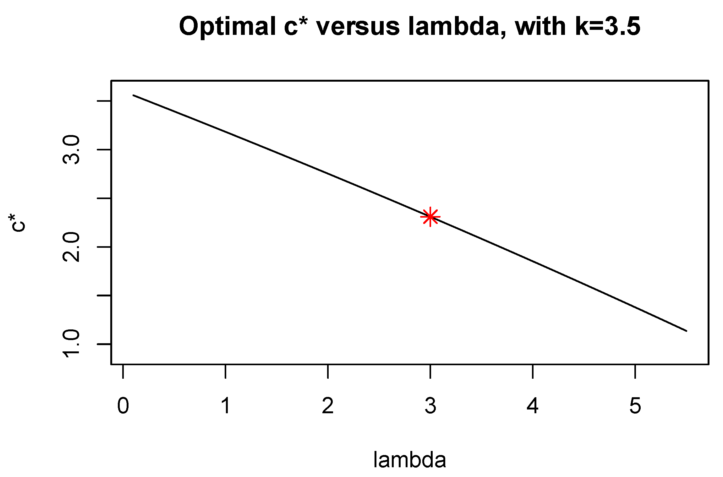
Lastly, to provide some context for these numerous parameters, we precisely set $\lambda =3$, $k=3.5$, $\theta =14$, and $\delta =-3.6$, so the initial default probability of the obligor is $P(A_T<0)\approx 0.03$. In practice, this is a realistic default risk, and the solution for this particular set of parameter values is $c^{*}\approx 2.31$, which can be seen in Figure 2, where the optimal (minimum) $c^{*}$ values are plotted for various $\lambda$. The decreasing relationship between $c^{*}$ and $\lambda$ is evident.

3.2. Modelling the Net Asset Value with Brownian Motion

We now consider the case of the net asset value process driven by Brownian motion. Concretely, we assume in this subsection that ${(A_t-A_0)}_{0\le t\le T}$ is a Brownian motion. With this modelling assumption, we can rephrase the objective function. We denote by $\mathsf{\Phi }$ and $\phi$ the cumulative distribution function and probability density function, respectively, of a standard normally distributed random variable. Since $G_t(x)=\mathsf{\Phi }\left(\frac{x}{\sqrt{t}}\right)$ in this case of Brownian motion, we immediately obtain from Proposition 1 the following result.

Proposition 3.

If ${(A_t-A_0)}_{0\le t\le T}$ is a Brownian motion, the function $f(c)$ in (3) can be written as

$$\begin{array}{cc}\hfill f(c)& =\sum _{j=1}^{N-1}(T-1-t_j)\frac{{\int }_{\frac{c-k}{\sqrt{t_j}}}^{\infty }\mathsf{\Phi }\left(\frac{-k-x\sqrt{t_j}}{\sqrt{T-t_j}}\right)\phi (x)dx}{\mathsf{\Phi }\left(\frac{-k}{\sqrt{T}}\right)}\hfill \\ & +\lambda \sum _{j=1}^{N-1}(T-1-t_j)({\int }_{-\infty }^{\frac{c-k}{\sqrt{t_{j-1}}}}\left(1-\mathsf{\Phi }\left(\frac{c-k-x\sqrt{t_{j-1}}}{\sqrt{t_j-t_{j-1}}}\right)\right)\phi (x)dx\hfill \\ & +{\int }_{\frac{c-k}{\sqrt{t_{j-1}}}}^{\infty }\mathsf{\Phi }\left(\frac{c-k-x\sqrt{t_{j-1}}}{\sqrt{t_j-t_{j-1}}}\right)\phi (x)dx).\hfill \end{array}$$

(9)

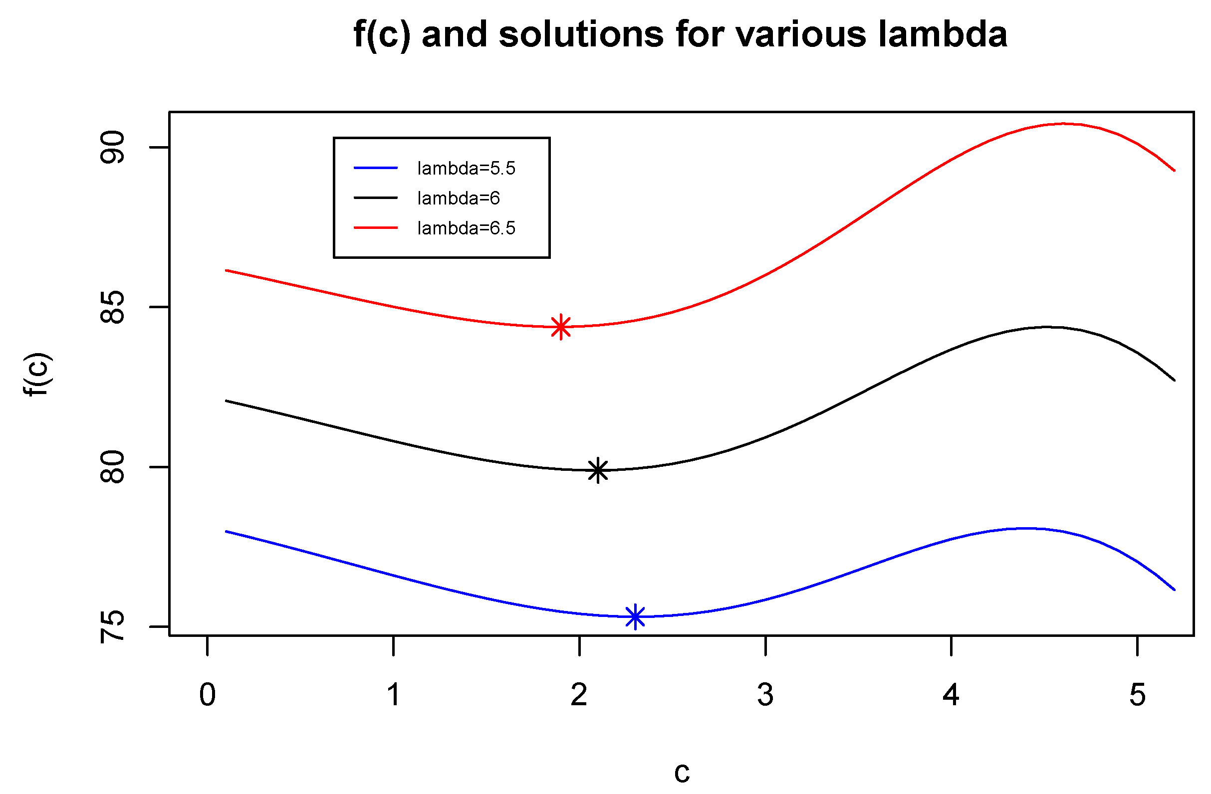
As Formula (9) is quite elaborate and complicated, arriving at an analytical solution relative to (3) is not feasible, although numerical results are certainly attainable. To demonstrate an example of the objective function and its relevant minimum, consider a loan issued over ten years $(T=10)$ with yearly reporting dates $(N=10)$, assuming equal time increments of $(t_j-t_{j-1})=1$ for $j\in \{1,2,\dots ,10\}.$ We fix the initial distance to default, k, such that $P(A_T<0)=0.05$. Accordingly, $P\left(\frac{A_T-A_0}{\sqrt{T}}<\frac{-k}{\sqrt{T}}\right)=0.05$ and $k=-\sqrt{T}{\mathsf{\Phi }}^{-1}(0.05)\approx 5.2.$ We observe the shape of the objective function for some reasonably chosen $\lambda$ values, and the respective solutions to the minimization problem, in Figure 3.

Note that, for this specific example, smaller values of the tuning parameter $(\lambda <5)$ produce solutions of $c^{*}\approx k\approx 5.2$, indicating the volatility portion is not properly weighted, since the early recognition of credit risk would be considered overwhelmingly important in that situation. Although an “ideal” selection of $\lambda$ is very subjective in terms of balancing the significance of the two portions of $f(c)$, the choices in this example clearly result in solutions existing in the desired interval of $0<c^{*}<k$. In addition, the decreasing relationship between $c^{*}$ and $\lambda$ is apparent, identical to the conclusion established in the previous subsection, where the shifted exponential distribution was used to model the net asset value.

4. Analyzing the Optimization Problem for Discrete Asset Distribution

4.1. Specific Increments

In a discrete-time framework, we can consider a situation where the increments $A_{t_j}-A_{t_{j-1}}$ are explicitly defined in terms of assuming possible values, along with their corresponding transition probabilities. In particular, we again consider the case where $T=t_N=t_2$, letting $t_1=\frac{T}{2}$ be the midpoint between the time the loan is issued and the time of maturity. Consistent with prior formulations, $A_{t_0}=A_0=k>0$, and, in this instance, the optimization problem corresponding to (3) is simplified as

$$\underset{c\le k}{min}f(c),$$

where

$$f(c)=\frac{T-2}{2}P\left(A_{\frac{T}{2}}>c|A_T<0\right)+\lambda \frac{T-2}{2}\left(P\left(A_{\frac{T}{2}}>c,A_0\le c\right)+P\left(A_{\frac{T}{2}}\le c,A_0>c\right)\right),$$

equivalent to

$$f(c)=\frac{T-2}{2}P\left(A_{\frac{T}{2}}>c|A_T<0\right)+\lambda \frac{T-2}{2}\left(P\left(A_{\frac{T}{2}}>c,k\le c\right)+P\left(A_{\frac{T}{2}}\le c,k>c\right)\right),$$

(10)

assuming again that $\lambda >0$. The increments are independent, with fixed transition probabilities

$$P\left(A_{\frac{T}{2}}-A_0=b_1\right)=P\left(A_T-A_{\frac{T}{2}}=b_2\right)=p_1>0.5,$$

$$P\left(A_{\frac{T}{2}}-A_0=-b_1\right)=P\left(A_T-A_{\frac{T}{2}}=-b_2\right)=1-p_1<0.5.$$

Here, we do not require identical distribution of the two increments, but impose $b_2>k>b_1>0$. We also specify $k+b_1-b_2<0<k-b_1+b_2$, which implies the initial default probability satisfies $P(A_T<0)={(1-p_1)}^2+p_1(1-p_1)=1-p_1<0.5$. Therefore, relative to a specific obligor, we select $p_1=1-P(A_T<0)$. Ultimately, the solution to the optimization problem, in terms of possible intervals for $c^{*}$, can be expressed as a piecewise function dependent on $\lambda$. We do consider the endpoints of the interval $0\le c^{*}\le k$ in this instance. The objective function is

$$f(c)=\left\{\begin{array}{cc}\frac{T-2}{2},\hfill & \mathrm{if}0\le c<k-b_1,\hfill \\ \frac{T-2}{2}\left(p_1+\lambda (1-p_1)\right),\hfill & \mathrm{if}k-b_1\le c<k,\hfill \\ \frac{T-2}{2}{p}_1(1+\lambda ),\hfill & \mathrm{if}c=k,\hfill \end{array}\right.$$

and, since the coefficient $\frac{T-2}{2}$ appears in each scenario, we examine all the other coefficients as a means of solving for the minimum of $f(c)$. First, we note that

$$p_1+\lambda (1-p_1)<p_1(1+\lambda )$$

regardless of the value of $\lambda$, since $1-p_1<p_1$ for our specified $p_1>0.5$. Therefore, we are certain that a solution of $c^{*}=k$ will not be chosen. Secondly, we see that $p_1+\lambda (1-p_1)<1$ if $\lambda <1$, for any $p_1>0.5$, leading to the clear solution to the minimization problem in terms of optimal $c^{*}$ selection intervals:

$$\mathrm{select}\left\{\begin{array}{cc}k-b_1\le c^{*}<k\hfill & \mathrm{if}\lambda <1,\hfill \\ \mathrm{any}0\le c^{*}<k\hfill & \mathrm{if}\lambda =1,\hfill \\ 0\le c^{*}<k-b_1\hfill & \mathrm{if}\lambda >1.\hfill \end{array}\right.$$

However, the instance when $\lambda =1$ provides us with no information other than $c^{*}\ne k$, while the case with $0\le c^{*}<k-b_1$ allows no opportunity to observe a possible IFRS 9 significant increase in credit risk prior to an eventual default. To conclude, choosing $0<\lambda <1$, resulting in a solution of $k-b_1\le c^{*}<k$, is most feasible in this setting.

4.2. General Increments

In this part, we still consider just two reporting dates, $\frac{T}{2}$ and T, but, in each period, we have K different possible values for the increments $A_{t_j}-A_{t_{j-1}}$, including $b_1,\dots ,b_K$, comprised of both positive and negative integers, with relevant probabilities $p_1,\dots ,p_K$. A general discrete random variable is modelled in each step, where we still assume that the changes in the two time steps are independent and identically distributed. In particular, we explicitly let X and Y be the independent random variables, in time order, so that $A_{\frac{T}{2}}=k+X$ and $A_T=k+X+Y$. To evaluate the objective function in this instance, starting with the recognition portion of $f(c)$, we compute

$$P\left[A_{\frac{T}{2}}>c|A_T<0\right]=\frac{P\left[A_{\frac{T}{2}}>c,A_T<0\right]}{P[A_T<0]}=\frac{P[X>c-k,X+Y<-k]}{P[X+Y<-k]}.$$

(11)

We simplify the denominator by splitting the event into disjoints parts, namely,

$$\begin{array}{cc}\hfill P[X+Y<-k]& =P\left[\bigcup _{n=1}^K\{X=b_n\}\cap \{X+Y<-k\}\right]\hfill \\ & =P\left[\bigcup _{n=1}^K\{X=b_n\}\cap \{b_n+Y<-k\}\right]\hfill \\ & =\sum _{n=1}^K{p}_{n}P[Y<-k-b_n]\hfill \\ & =\sum _{n=1}^K{p}_n\sum _{\{\ell :b_{\ell }<-k-b_n\}}{p}_{\ell },\hfill \end{array}$$

using the independence of X and Y in the penultimate step. In an analogous way, the numerator in (11) can be written as

$$P[X>c-k,X+Y<-k]=\sum _{\{n:b_n>c-k\}}{p}_n\sum _{\{\ell :b_{\ell }<-k-b_n\}}{p}_{\ell }$$

so that Formula (11) becomes

$$P\left[A_{\frac{T}{2}}>c|A_T<0\right]=\frac{P[X>c-k,X+Y<-k]}{P[X+Y<-k]}=\frac{{\sum }_{\{n:b_n>c-k\}}{p}_n{\sum }_{\{\ell :b_{\ell }<-k-b_n\}}{p}_{\ell }}{{\sum }_{n=1}^K{p}_n{\sum }_{\{\ell :b_{\ell }<-k-b_n\}}{p}_{\ell }}.$$

Under the assumption that $A_0=k>c$, from the volatility portion of $f(c)$, we have that

$$\begin{array}{cc}\hfill P\left(A_{\frac{T}{2}}\le c\right)& =P[X\le c-k]\hfill \\ & =\sum _{n=1}^{K}P[\{X=b_n\}\cap \{X\le c-k\}]\hfill \\ & =\sum _{\{n:b_n\le c-k\}}P[X=b_n]\hfill \\ & =\sum _{\{n:b_n\le c-k\}}{p}_n,\hfill \end{array}$$

resulting in Formula (10) being expressed in this setting as

$$\begin{array}{cc}\hfill f(c)& =\frac{T-2}{2}\frac{{\sum }_{\{n:b_n>c-k\}}{p}_n{\sum }_{\{\ell :b_{\ell }<-k-b_n\}}{p}_{\ell }}{{\sum }_{n=1}^K{p}_n{\sum }_{\{\ell :b_{\ell }<-k-b_n\}}{p}_{\ell }}+\lambda \frac{T-2}{2}\sum _{\{n:b_n\le c-k\}}{p}_n\hfill \\ & =\frac{T-2}{2}\left[\frac{{\sum }_{\{n:b_n>c-k\}}{p}_n{\sum }_{\{\ell :b_{\ell }<-k-b_n\}}{p}_{\ell }}{{\sum }_{n=1}^K{p}_n{\sum }_{\{\ell :b_{\ell }<-k-b_n\}}{p}_{\ell }}+\lambda \sum _{\{n:b_n\le c-k\}}{p}_n\right]\hfill \\ & =\frac{T-2}{2}\left[\frac{{\sum }_{\{n:b_n>c-k\}}{p}_n{\sum }_{\{\ell :b_{\ell }<-k-b_n\}}{p}_{\ell }+{\sum }_{n=1}^K{p}_n{\sum }_{\{\ell :b_{\ell }<-k-b_n\}}{p}_{\ell }\left(\lambda {\sum }_{\{n:b_n\le c-k\}}{p}_n\right)}{{\sum }_{n=1}^K{p}_n{\sum }_{\{\ell :b_{\ell }<-k-b_n\}}{p}_{\ell }}\right].\hfill \end{array}$$

Notice that the expression for $f(c)$ depends on c only in the index sets in two of the summations. This implies that $f(c)$ is piecewise constant with jumps when $c=b_n+k$ for $n=1,\dots ,N$. Furthermore, the sum ${\sum }_{\{n:b_n>c-k\}}{p}_n$ is decreasing in c, as it relates to the early recognition of credit risk. On the contrary, the sum ${\sum }_{\{n:b_n\le c-k\}}{p}_n$ in the second term of the numerator of the objective function, is increasing in c, being part of the volatility portion. As a result, the optimal $c^{*}$ is chosen in an interval between $b_n+k$ and $b_{n+1}+k$ such that the expression for $f(c)$ on this interval is minimal compared to values on other intervals. Therefore, the solution is similar to that in Section 4.1, but more intricate and cumbersome. Due to the complexity of this expression, which depends on the exact distance to default along with the incremental and probability values, a computer program is required to select the minimum numerically. For each n, it will select $c_n$ with $b_n+k\le c_n<b_{n+1}+k$ and compute $f(c_n)$. Because f is constant on such intervals, the specific choice of $c_n$ within the interval does not affect the value of $f(c_n)$. Among all $f(c_n)$ for different n, the program will choose the one with the smallest value, say $f(c_{n^{*}})$, as the minimum.

5. Relating Our Model to the European Union Stress Test and Standard and Poor’s Default Data

For this section, we use the assumption from Section 3.2 regarding the net asset value modelling, such that ${(A_t-A_0)}_{0\le t\le T}$ is a Brownian motion, and apply it in practical settings.

5.1. Selection of $\lambda$ in Comparison to European Union Framework

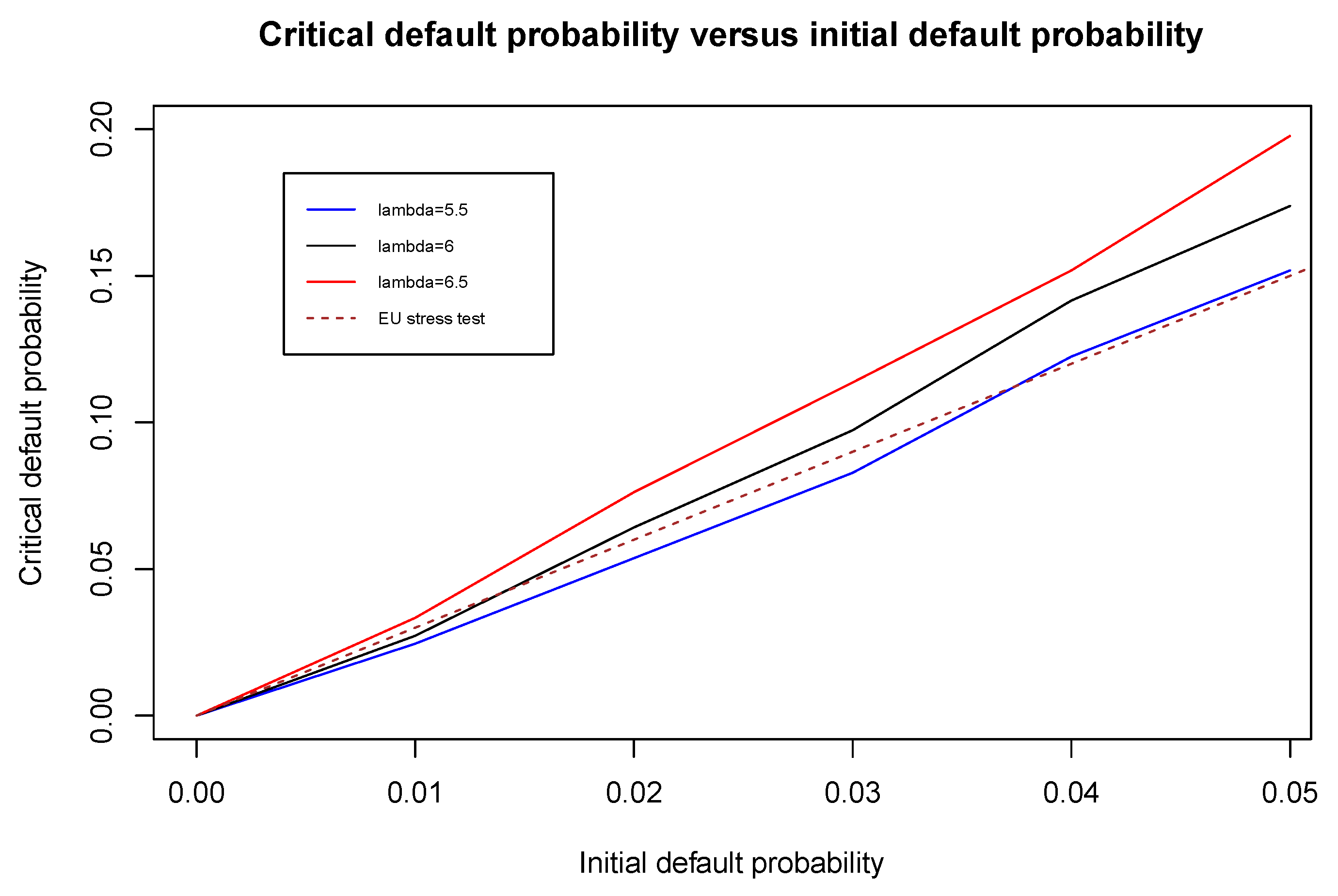
A basic criticism of the trade-off modelled in our problem formulation is that the tuning parameter $\lambda$ could be chosen in a subjective manner by a financial institution, based on the extent to which they are concerned about minimizing income volatility as compared to recognizing credit risk earlier. To justify what reasonable values for $\lambda$ are in practice, we make a comparison with a European Union (EU) definition. Although IFRS 9 does not specify explicitly what constitutes a significant increase, the stress test framework of the European Banking Authority (2018) defines a significant increase in credit risk as being 200% from the initial credit risk. To convert this definition into our setting, consider a loan with maturity T and current time t, so that the remaining time to maturity is $T-t$. The lifetime default probability at the initial time is $P(A_T<0)=\mathsf{\Phi }\left(\frac{-k}{\sqrt{T}}\right)$. Assuming that the net asset value $A_t$ equals a at time t, the lifetime default probability at time t is

$$P(A_T<0|A_t=a)=P(A_t+A_T-A_t<0|A_t=a)=P(a+W_{T-t}<0)$$

for a Brownian motion ${(W_t)}_{0\le t\le T}$. We use the property of Brownian motion that $P(W_T-W_t\le a)=P(W_{T-t}\le a)$ for any constant $a.$ Since $W_{T-t}$ is normally distributed with mean zero and variance $T-t$, we obtain that $P(a+W_{T-t}<0)=\mathsf{\Phi }\left(\frac{-a}{\sqrt{T-t}}\right)$. By the framework of the EU stress test, the risk of a loan has significantly increased if the current lifetime default probability is at least triple the initial lifetime default probability, which means $P(a+W_{T-t}<0)\ge 3P(A_T<0)$. We now define $a^{*}$ as the critical value so that $P(a^{*}+W_{T-t}<0)=3P(A_T<0)$. Assuming the loan is in the middle of the lifetime, such that $t=\frac{T}{2}$, we compare $P(a^{*}+W_{T-t}<0)$ with the corresponding value $P(c^{*}+W_{T-t}<0)$ for our optimizer $c^{*}$. For various k values, these solutions are determined numerically, using the objective function representation in (9). Figure 4 conveys an example of the relationship between the initial lifetime default probability $P(A_T<0)$ and the critical lifetime default probability $P\left(c^{*}+W_{\frac{T}{2}}<0\right),$ with $t=\frac{T}{2}$. A positive relationship exists for each $\lambda$ value shown, since the critical lifetime default probability increases, intuitively, as the initial lifetime default probability increases. In comparison to the EU stress test reference line, we see that, for each $\lambda$, the relationship does not appear to be perfectly linear. However, we can still feasibly suggest that the value $P(a^{*}+W_{T-t}<0)$ from the stress test threshold corresponds to a parameter choice of $\lambda$ between 5.5 and 6.5, for this loan with maturity of $T=10$. It is not critical for us to choose $\lambda$ completely analogously to the EU framework. Rather, this comparison is made in order to explain how values of the tuning parameter can be inferred as a guideline for practical applications of our framework.

5.2. Analyzing the Income Volatility Portion with Default Data by Standard and Poor’s

To directly relate our model to recent financial data, we use Standard and Poor’s (2018) global corporate average default rates and yearly credit grouping transition rates. Each defined credit rating group has assigned one-year and lifetime probabilities of default, based on corporate averages from 1981 to 2017, which is relevant for any future length of time up until maturity of a loan. Additionally, yearly transition probabilities to all possible credit rating groups are available. From this information, evaluating what percentage of loans experience a significant increase in credit risk, depending on the threshold $c^{*}$, is critical in terms of determining the severity of income volatility for a bank in a particular year.

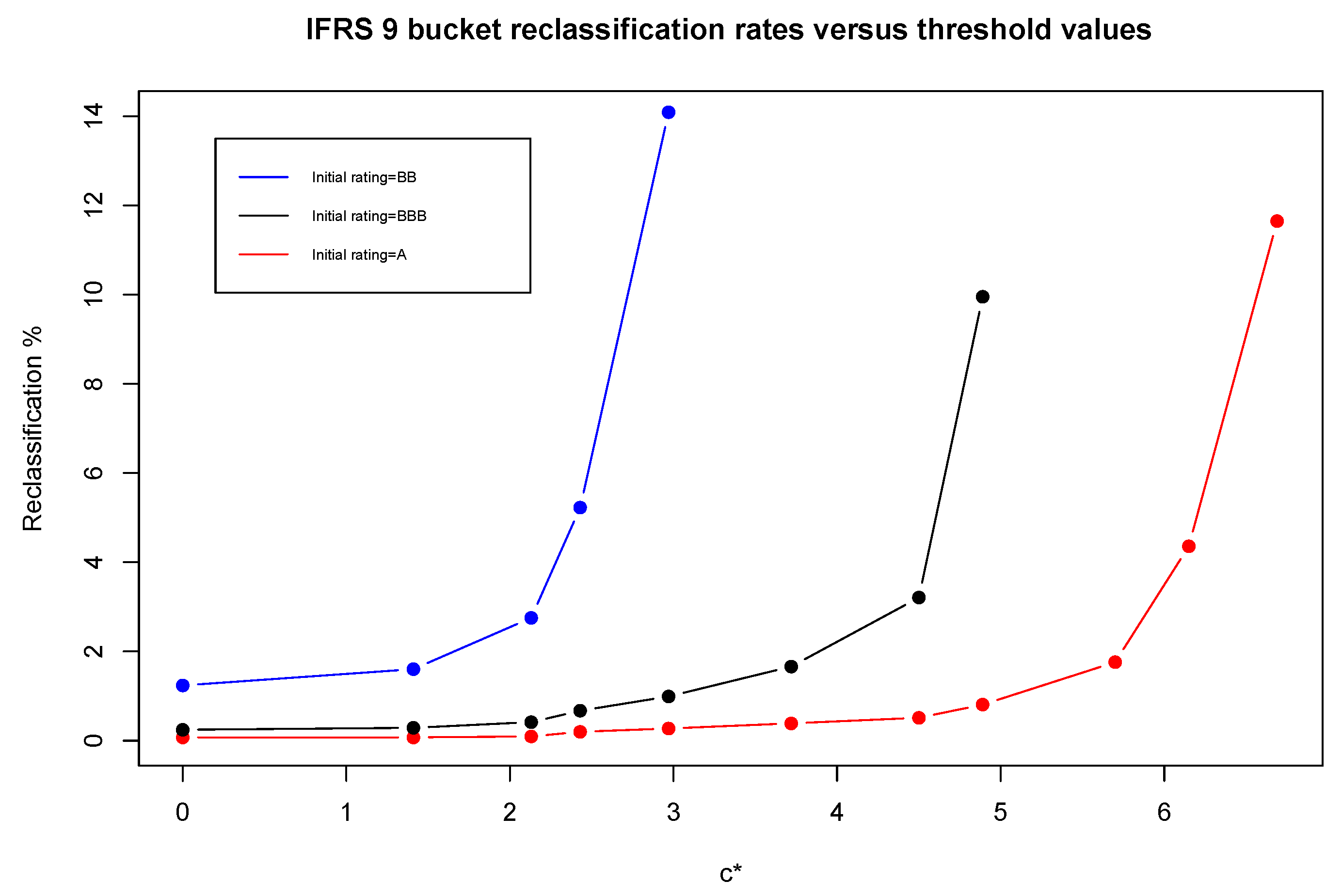
As far as integrating this data into our problem formulation, we first specify an initial rating group, and subsequently observe the performance at time $t=1$ year of a loan issued over $T=10$ years. The transition rates reveal proportions of loans in each respective rating group possessing lower credit quality, one year since origination. Furthermore, under the modelling structure of Section 5.1, possible threshold solutions are approximated using $P(c^{*}+W_{T-t}<0)=P(c^{*}+W_{10-1}<0)=P(c^{*}+W_9<0)$, in which nine-year probabilities of default over the remaining time to maturity are used, relative to the current credit rating group at time $t=1$. For various $c^{*}$ values defined by the cutoff points described by progressive downgrades in credit rating groups, the yearly transition rates reveal the percentage of loans that would transfer to an IFRS 9 bucket of worsened performance status. Assuming each loan examined originated in bucket 1, and that $c^{*}<k$, Figure 5 displays the influence of the threshold level on the IFRS 9 bucket reclassification rate, for three different initial rating groups.

With an initial rating group of A, the initial distance to default for a ten-year loan is $k=-\sqrt{10}{\mathsf{\Phi }}^{-1}(0.0147)\approx 6.89$, and if we attribute, for example, a significant increase in credit risk over a one-year period being a downgrade to rating BBB or worse, then $c^{*}=-\sqrt{9}{\mathsf{\Phi }}^{-1}(0.0285)\approx 5.71$. From our illustration, it is evident that the loan reclassification rate from one-year ECL to lifetime ECL is more profound for lower initial credit rating groups (such as BB), meaning these obligors that have a higher risk of non-payment also contribute significantly to increased income volatility for the bank that issues their loans.

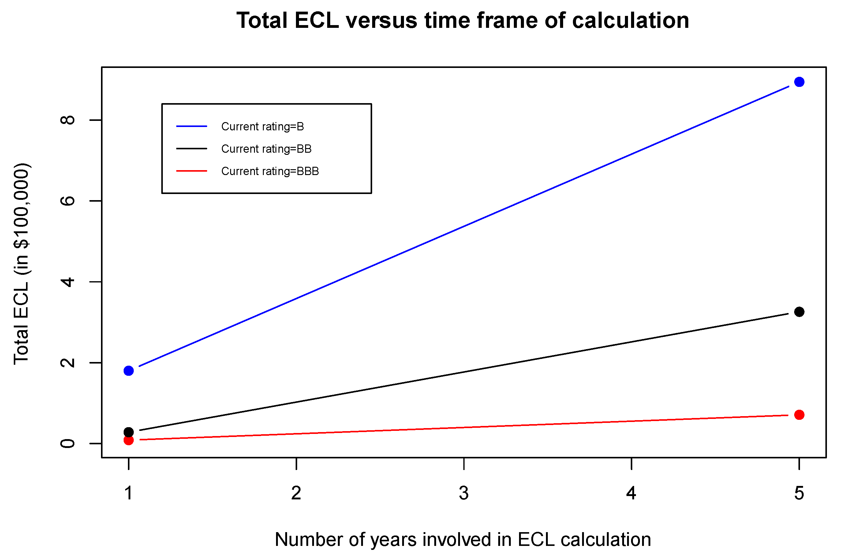
The actual calculation of ECL involves sophisticated models for each component, including PD, EaD, and LGD for a credit facility. For demonstration purposes, a proxy ECL calculation can be created to exemplify the relationship between ECL and IFRS 9 loan reclassification, incorporating the same default data from Standard and Poor’s (2018). We still consider the case when $T=10$, and assess three different samples of 100 similar loans having the same initial and current rating group, namely ratings A, BBB, and BB for the three samples, as of the midpoint of $T=5$ years. After year 5, we have three samples of 100 loans each, with one sample experiencing a common migration from rating group A to BBB, the second showing a deterioration from rating group BBB to BB, and the third having a transition from rating group BB to B. In summary, all 100 obligors in a particular sample have undergone a credit quality downgrade of three notches. We then fix $\mathrm{EaD}=\$500,000$ and $\mathrm{LGD}=0.1$, and use both one-year and lifetime PDs (for the five remaining years to maturity) to calculate proxy ECLs, simply from the product of the three components. Figure 6 emphasizes the difference between one-year and lifetime ECL for each sample from an initial rating group, assuming all loans originated in IFRS 9 bucket 1.

Essentially, if a downgrade of three rating groups is deemed sufficient enough to constitute a significant increase in credit risk, lifetime (five-year) ECL is computed. Otherwise, ECL for a one-year horizon is calculated. Consistent with the interpretation of Figure 5, we observe that the effect of reclassification from bucket 1 to bucket 2 is considerably more drastic for inferior rating groups. Clearly, the total ECL for a sample of just 100 loans increases sharply, by over $700,000, when current rating group B, corresponding to initial rating group BB, is classified in IFRS 9 bucket 2 rather than bucket 1.

6. Conclusions

The late recognition of credit losses was a major criticism of accounting of financial assets during the global financial crisis of 2007–2008. The introduction of IFRS 9 addressed this issue by requiring banks to build provisions for the lifetime ECL, rather than one-year ECL, when the credit risk of a loan has significantly increased. However, IFRS 9 poses the challenging task to banks of defining what exactly such a significant increase in credit risk means for each of their loans. Such a definition embeds the trade-off between early recognition of credit risk and income volatility, which is the downside of frequently reclassifying loans between buckets to account for either one-year or lifetime ECL.

Our approach to introduce and analyze a statistical framework that models this trade-off makes three contributions to the discussion on implementing IFRS 9 and, more broadly, on the provisioning of ECL. First, it helps better understand how different factors in credit risk management affect the optimal threshold for what should be considered a significant increase in credit risk. Second, banks can use our framework to define significant increases in credit risk consistently across different loans. Finally, regulators may use our framework to better compare the banks’ different definitions of significant increases in credit risk. Because IFRS 9 does not define what constitutes a significant increase in credit risk, our framework gives flexibility to specify the relative importance of early recognition of credit risk compared to reduction of income volatility, although we showed how information about stress tests, such as that of the European Banking Authority (2018), helps as a guideline for the parameter specification.

Beyond the application to IFRS 9, our work shows how interesting research questions emerge: in response to economic and political developments, accounting standards are introduced and revised, which may require mathematical models and lead to statistical questions. Possible future studies in this area at the intersection of accounting and statistics include implementation questions about IFRS 15, which became effective 1 January 2018 and provides guidance on revenue accounting from contracts with customers. IFRS 15 requires operational models for revenues and contract assessments; see PricewaterhouseCoopers (2018). Similarly, accounting of share-based payments to employees may require mathematical and statistical models, as per IFRS 2; see Ernst & Young (2015). Under IFRS 17, whose proposed effective date is 1 January 2022, liabilities from insurance contracts will be calculated using a present-value model with provisions for risk; see PricewaterhouseCoopers (2016). In all such applications, mathematical models together with statistical techniques can provide useful quantitative assessments, but also have limitations. Inevitably, they come with model risk and statistical errors so that they need to be applied in a reasonable way, combined with qualitative assessments.

References

- Angilella, Silvia, and Sebastiano Mazzù. 2017. A credit risk model with an automatic override for innovative small and medium-sized enterprises. Journal of the Operational Research Society, 1–17. [Google Scholar] [CrossRef]
- Basel Committee on Banking Supervision. 2005. An Explanatory Note on the Basel II IRB Risk Weight Functions. Bank for International Settlements. Available online: www.bis.org (accessed on 5 April 2019).
- Basel Committee on Banking Supervision. 2015. Guidance on Credit Risk and Accounting for Expected Credit Losses. Bank for International Settlements. Available online: www.bis.org (accessed on 5 April 2019).
- Bluhm, Christian, and Ludger Overbeck. 2003. Systematic risk in homogeneous credit portfolios. In Credit Risk: Measurement, Evaluation and Management (Contributions to Economics). Edited by Georg Bol, Gholamreza Nakhaeizadeh, Svetlozar T. Rachev, Thomas Ridder and Karl-Heinz Vollmer. Berlin/Heidelberg: Springer, pp. 35–48. [Google Scholar]
- Bluhm, Christian, Ludger Overbeck, and Christoph Wagner. 2010. An Introduction to Credit Risk Modeling, 2nd ed. Boca Raton: Chapman & Hall/CRC. [Google Scholar]
- Bohn, Jeffrey R., and Roger M. Stein. 2009. Active Credit Portfolio Management in Practice. Hoboken: Wiley Finance. [Google Scholar]
- Cohen, Benjamin H., and Gerald A. Edwards Jr. 2017. The New Era of Expected Credit Loss Provisioning. BIS Quarterly Review. Available online: www.bis.org (accessed on 5 April 2019).
- Crook, Jonathan N., David B. Edelman, and Lyn C. Thomas. 2007. Recent developments in consumer credit risk assessment. European Journal of Operational Research 183: 1447–65. [Google Scholar] [CrossRef]
- Ernst & Young. 2015. Accounting for Share-Based Payments under IFRS 2—The Essential Guide. Available online: www.ey.com (accessed on 5 April 2019).
- European Banking Authority. 2017. Report on Results from the Second EBA Impact Assessment of IFRS 9. Available online: www.eba.europa.eu (accessed on 5 April 2019).
- European Banking Authority. 2018. 2018 EU-Wide Stress Test. European Union. Available online: www.eba.europa.eu (accessed on 5 April 2019).
- Frei, Christoph, and Marcus Wunsch. 2018. Moment estimators for autocorrelated time series and their application to default correlations. Journal of Credit Risk 14: 1–29. [Google Scholar] [CrossRef]
- Gordy, Michael B. 2000. A comparative anatomy of credit risk models. Journal of Banking and Finance 24: 119–49. [Google Scholar] [CrossRef]
- Kallenberg, Olav. 2002. Foundations of Modern Probability, 2nd ed. Berlin/Heidelberg: Springer. [Google Scholar]
- Kumar, P. Ravi, and Vadlamani Ravi. 2007. Bankruptcy prediction in banks and firms via statistical and intelligent techniques—A review. European Journal of Operational Research 180: 1–28. [Google Scholar] [CrossRef]
- Maggi, Filippo, Alfonso Natale, Theodore Pepanides, Enrico Risso, and Gerhard Schröck. 2017. IFRS 9: A Silent Revolution in Banks’ Business Models. New York: McKinsey & Company. [Google Scholar]
- McNeil, Alexander J., Rüdiger Frey, and Paul Embrechts. 2015. Quantitative Risk Management: Concepts, Techniques and Tools, rev. ed. Princeton: Princeton University Press. [Google Scholar]
- Merton, Robert C. 1974. On the pricing of corporate debt: The risk structure of interest rates. Journal of Finance 29: 449–70. [Google Scholar]
- Miu, Peter, and Bogie Ozdemir. 2009. Stress-testing probability of default and migration rate with respect to Basel II requirements. Journal of Risk Model Validation 3: 1–36. [Google Scholar] [CrossRef]
- Miu, Peter, and Bogie Ozdemir. 2017. Adapting the Basel II advanced internal-ratings-based models for International Financial Reporting Standard 9. Journal of Credit Risk 13: 53–83. [Google Scholar] [CrossRef]
- PricewaterhouseCoopers. 2016. The Wait Is Nearly Over? IFRS 17 Is Coming, Are You Prepared for It? Available online: www.pwc.com (accessed on 5 April 2019).
- PricewaterhouseCoopers. 2018. Revenue from Contracts with Customers. Available online: www.pwc.com (accessed on 5 April 2019).
- Randall, Mark, and Sandra Thompson. 2017. IFRS 9 Impairment: Significant Increase in Credit Risk: PwC in Depth. Available online: www.pwc.com (accessed on 5 April 2019).
- Simons, Dietske, and Ferdinand Rolwes. 2009. Macroeconomic default modeling and stress testing. International Journal of Central Banking 5: 177–204. [Google Scholar]
- Skoglund, Jimmy, and Wei Chen. 2016. The application of credit risk models to macroeconomic scenario analysis and stress testing. Journal of Credit Risk 12: 1–45. [Google Scholar] [CrossRef]
- Standard and Poor’s. 2018. Default, Transition, and Recover: 2017 Annual Global Corporate Default Study and Rating Transitions. Available online: www.spratings.com (accessed on 5 April 2019).
- Stulz, Rene M. 2015. Risk-taking and risk management by banks. Journal of Applied Corporate Finance 27: 8–18. [Google Scholar] [CrossRef]
- Yang, Bill Huajian, and Zunwei Du. 2015. Stress testing and modeling of rating migration under the Vasicek model framework: Empirical approaches and technical implementation. Journal of Risk Model Validation 9: 33–47. [Google Scholar] [CrossRef]
Figure 1.
Simulation of net asset value of an obligor, with and , arbitrarily chosen, for a ten-year loan. is modelled by Brownian motion in this illustration.
Figure 2.
Solutions, , versus corresponding values, with , and . A specific solution, for is labelled in red.
Figure 3.
Plot of for various , with , , and . The solutions, determined numerically, are (), () and ().
Figure 4.
Plot of versus , for various , with . The dashed line shows the relationship outlined by the EU stress test, which is linear by definition.
Figure 5.
Plot of reclassification percentage from IFRS 9 bucket 1 to buckets 2 or 3, after year one of a ten year loan, for different initial ratings based on Standard and Poor’s global corporate averages from 1981–2017.
Figure 6.
Plot of total ECL versus number of years involved in the calculation, for samples of 100 loans grouped in the same rating at the midpoint of a ten year loan. For each of the three current rating groups shown, we assume that these loans originated in IFRS 9 bucket 1, with the same initial rating.