Loss Reserving Models: Granular and Machine Learning Forms

School of Risk and Actuarial Studies, University of New South Wales, Kensington, NSW 2052, Australia
Risks 2019, 7(3), 82; https://0-doi-org.brum.beds.ac.uk/10.3390/risks7030082
Submission received: 10 May 2019
/
Revised: 12 June 2019
/
Accepted: 18 June 2019
/
Published: 19 July 2019
(This article belongs to the Special Issue Claim Models: Granular Forms and Machine Learning Forms)
Abstract
:The purpose of this paper is to survey recent developments in granular models and machine learning models for loss reserving, and to compare the two families with a view to assessment of their potential for future development. This is best understood against the context of the evolution of these models from their predecessors, and the early sections recount relevant archaeological vignettes from the history of loss reserving. However, the larger part of the paper is concerned with the granular models and machine learning models. Their relative merits are discussed, as are the factors governing the choice between them and the older, more primitive models. Concluding sections briefly consider the possible further development of these models in the future.
1. Background
The history of loss reserving models, spanning 50-odd years, displays a general trend toward ever-increasing complexity and data-intensity. The objectives of this development have been broadly two-fold, both drawing on increased richness of the data. One objective has been increased predictive power; the other the enablement of modelling of the micro-mechanisms of the claim process (which may also enhance predictive power).
Two families of model that have undergone development within this context over the past decade are granular models (GMs) and machine learning models (MLMs). The first of these, also known as micro-models, is aimed at the second objective above. As the complexity of model structures increases, feature selection and parameter estimation also become more complex, time-consuming and expensive. MLMs are sometimes seen as a suitable means of redress of these difficulties.
The purpose of the present paper is to survey the history of loss reserving models, and how that history has led to the most recent types of model, granular forms and machine learning forms. History has not yet resolved whether one of these forms is superior to the other, or whether they can coexist in harmony. To some extent, therefore, they are currently in competition with each other.
Claim models may be developed for purposes other than loss reserving, with different imperatives. For example, pricing will require differentiation between individual risks, which loss reserving may or may not require. Here, emphasis will be placed on loss reserving applications throughout. The performance of the models considered here might be evaluated differently in relation to other applications.
Much of the historical development of loss reserving models has been, if not driven, at least enabled by the extraordinary increase in computing capacity that has occurred over the past 50 years or so. This has encouraged the analysis of more extensive data and the inclusion of more features in models.
Some of the resulting innovations have been of obvious benefit. However, the advantages and disadvantages of each historical model innovation will be discussed here, and this will create a perspective from which one may attempt to anticipate whether one of the two model forms is likely to gain ascendancy over the other in the near future.
Section 3, Section 4, Section 5 and Section 6 proceed through the archaeology of loss reserving models. Archaeological ages are identified, marking fundamental breaks in model evolution. These sections proceed roughly chronologically, discussing many of the families of models contained in the literature, identifying their relative advantages and disadvantages.
These historical perspectives sharpen one’s perspective on the issues associated with the more modern GMs and MLMs. They expose the strengths and weaknesses of earlier models, and place in focus those areas where the GMs and MLMs might have potential for improved methodology.
Against this background, Section 7 discusses the criteria for model selection, and Section 8 concentrates on the predictive efficiency of GMs and MLMs. Section 8 also discusses one or two aspects of MLMs that probably require resolution before those models will be widely accepted, and Section 9 and Section 10 draw the discussion of the previous sections together to reach some conclusions and conjectures about the future.
It is not the purpose of this paper to provide a summary of an existing methodology. This is provided by various texts. The real purpose is set out in the preceding paragraph, and the discussion of historical model forms other than GMs or MLMs is introduced only to provide relevant context to the GM–MLM comparison.
Thus, a number of models will be introduced without, or with only brief, description. It is assumed that the reader is either familiar with the relevant detail or can obtain it from the cited reference.
2. Notation and Terminology
This paper will consider numerous models, with differing data requirements. The present section will establish a relatively general data framework that will serve for most of these models. All but the most modern of these are covered to some degree in the standard loss reserving texts, Taylor (1986, 2000) and Wüthrich and Merz (2008).
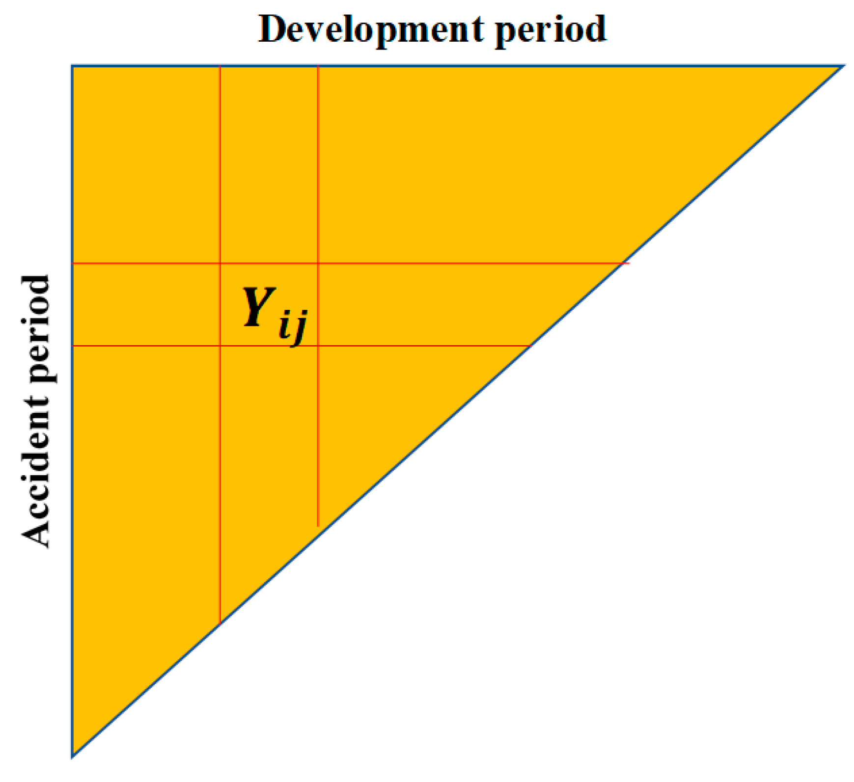
Claim data may relate to individual or aggregate claims, but will often be labelled by accident period and development period. These periods are not assumed to be years, but it is assumed that they are all of equal duration, e.g., accident quarter and development quarter. Other cases are possible, e.g., accident year and development quarter, but add to the notational complexity while adding little insight to the discussion.
Let denote claim payments in development period in respect of claim , which was incurred in accident period . The couple will be referred to as a cell. Also, define the total claim payments associated with the cell as
Usually, will be considered to be a random variable, and a realization of it will be denoted by . Likewise, a realisation of will be denoted by . As a matter of notation, and .
Many simple claim models use the conventional data triangle, in which cells exist for and , which may be represented in triangular form with and indexing rows and columns, respectively, as illustrated in Figure 1.
It is useful to note at this early stage that the cell falls on the -th diagonal of the triangle. Payments occurring anywhere along this diagonal are made in the same calendar period, and accordingly diagonals are referred to as calendar periods or payment periods.
It will be useful, for some purposes, to define cumulative claim payments. For claim , from accident period , the cumulative claim payments to the end of development period are defined as
and the definition is extended in the obvious way to , the aggregate, for all claims incurred in accident period , of cumulative claim payments to the end of development period .
A quantity of interest later is the operational time (OT) at the finalisation of a claim. OT was introduced to the loss reserving literature by Reid (1978), and is discussed by Taylor (2000) and Taylor and McGuire (2016).
Let the OT for claim be denoted , defined as follows. Suppose that claim belongs to accident period , and that is an estimator of the number of claims incurred in this accident period. Let denote the number of claims from the accident period finalised up to and including claim . Then . In other words, is the proportion of claims from the same accident period as claim that are finalised up to and including claim .
3. The Jurassic Period
The earliest models date generally from the late 1960s. These include the chain ladder and the separation method, and all their derivatives, such as Bornhuetter–Ferguson and Cape Cod. They are discussed in Taylor (1986, 2000) and Wüthrich and Merz (2008). The chain ladder’s provenance seems unclear, but it may well have preceded the 1960s.
These models were based on the notion of “development” of an aggregate of claims over time, i.e., the tendency for the total payments made in respect of those claims to increase over time in accordance with some recognisable pattern. They therefore fall squarely in the class of phenomenological, or non-causal, models, in which attention is given to only mathematical patterns in the data rather than the mechanics of the claim process or any causal factors.
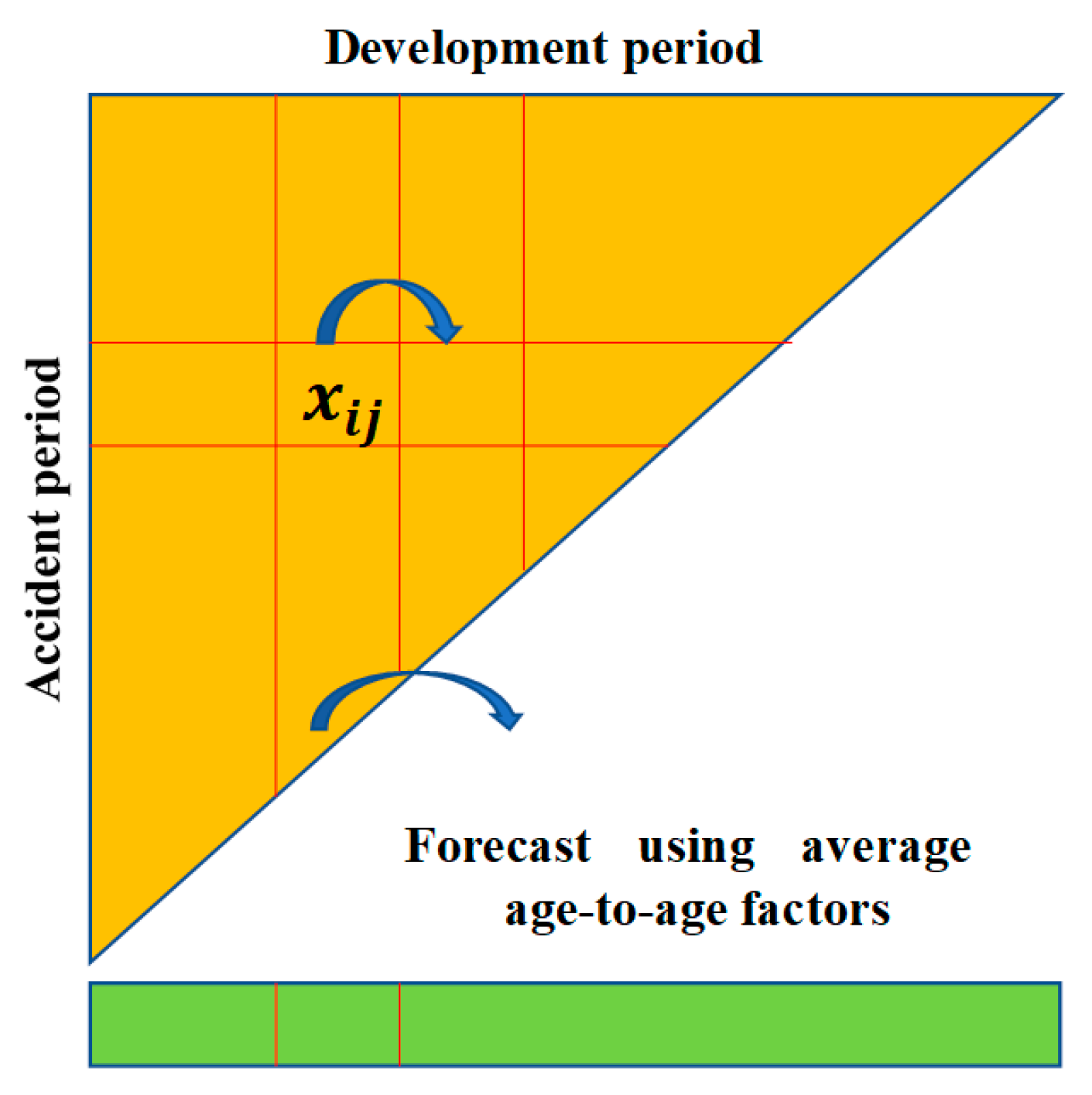
Figure 2 is a slightly enhanced version of Figure 1, illustrating the workings of the chain ladder. It is assumed that a cell develops to its successor in accordance with the rule
where is a parameter describing development, and referred to as a development factor or an age-to-age factor.
Forecasts are made according to this rule. The trick is to estimate factors from past experience, and in practice they were typically estimated by some kind of averaging of past observations on these factors, i.e., observed values of .
Models of this type are very simple, but their most interesting quality is that they are not, in fact, models at all. The original versions of these models were not stochastic, as is apparent from (1). Nor is (1) even true over the totality of past experience; it is not the case for a typical data set that , constant for fixed , but varying . So, the “models” in this group are actually algorithms rather than models in the true sense.
Of course, this fault has been rectified over the subsequent years, with (1) replaced by the genuine model defined by the following conditions:
- (a)
- Each row of the triangle is a Markov chain.
- (b)
- Distinct rows of the triangle are stochastically independent.
- (c)
- is subject to some defined distribution for which , where is a parameter to be estimated from data.
A model of this sort was proposed by Mack (1993) (“the Mack model”), and much development of it has followed, though the earliest stochastic formulation of the chain ladder (Hachemeister and Stanard 1975) should also be credited.
While the formulation of a genuine chain ladder model was immensely useful, the fundamental structure of the model retains some shortcomings. First, in statistical parlance, it is a multiplicative row-and-column effect model. This is a very simple structure, in which all rows are just, in expectation, scalar multiples of one another. This lacks the complexity to match much real-life claim experience.
For example, a diagonal effect might be present, e.g., in (c), where is a parameter specific to diagonal . A variable inflationary effect would appear in this form, but cannot be accommodated in the chain ladder model formulated immediately above. One can add such parameters to the model, but this will exacerbate the over-parameterisation problem described in the next main dot point.
Rates of claim settlement might vary from one row to another, causing variation in the factors (Fisher and Lange 1973). Again, one can include additional effects in the models, but at the expense of additional parameters.
Second, even with this simple form, it is at risk of over-parameterisation. The model of an triangle and the associated forecast are characterised by parameters, (actually, the last of these are conditioning observations but function essentially as parameters in the forecast). For example, a triangle would contain 55 observations, would forecast 45 cells, and would require 18 parameters. Over-parameterisation can increase forecast error.
The Jurassic continued through the 1970s and into the 1980s, during which time it spawned mainly non-stochastic models. It did, however, produce some notably advanced creatures. Hachemeister and Stanard (1975) has already been mentioned. A stochastic model of claim development essentially by curve fitting was introduced by Reid (1978), and Hachemeister (1978, 1980) constructed a stochastic model of individual claim development.
4. The Cretaceous Period—Seed-Bearing Organisms Appear
The so-called models of the Jurassic period assumed the general form:
where is some real-valued function, is the vector containing the entire set of observations as its components, and α is some set of parameters, either exogenous or estimated from . The case of the chain ladder represented by (1) is an example in which .
Although (2) is not a stochastic model, it may be converted to one by the simple addition of a stochastic error εij:
Note that the Mack model of Section 3 is an example. In addition, with some limitation of and εij, (3) becomes a Generalised Linear Model (GLM) (McCullagh and Nelder 1989), specified as follows:
- (a)
- and is a distribution contained in the exponential dispersion family (EDF) (Nelder and Wedderburn 1972) with dispersion parameter and weights ;
- (b)
- takes the parametric form for some one–one function (called the link function), and where is a vector of covariates associated with the cell and the corresponding parameter vector.
Again, the chain ladder provides an example. The choices yield the Mack model of Section 3.
The Cretaceous period consisted of such models. The history of actuarial GLMs is longer than is sometimes realised. Its chronology is as follows:
- in 1972, the concept was introduced by Nelder and Wedderburn;
- in 1977, modelling software called GLIM was introduced;
- in 1984, the Tweedie family of distributions was introduced (Tweedie 1984), simplifying the modelling software;
- in 1990 and later, seminal actuarial papers (Wright 1990; Brockman and Wright 1992) appeared.
GLMs were not widely used in an actuarial context until 1990, and to some extent this reflected the limitations of earlier years’ computing power. It should be noted that their actuarial introduction to domestic lines pricing occurred as early as 1979 (Baxter et al. 1980). I might be permitted to add here a personal note that they were heavily used for loss reserving in all the consultancies with which I was associated from the early 1980s.
The range of GLM loss reserving applications has expanded considerably since 1990. A few examples are:
- analysis of an Auto Liability (relatively long-tailed) portfolio (Taylor and McGuire 2004) with:
- ○
- rates of claim settlement that varied over time;
- ○
- superimposed inflation (SI) (a diagonal effect) that varied dramatically over time and also over OT (defined in Section 2);
- ○
- a change of legislation affecting claim sizes (a row effect);
- analysis of a mortgage insurance portfolio (Taylor and Mulquiney 2007), using a cascade of GLM sub-models of experience in different policy states, viz.
- ○
- healthy policies;
- ○
- policies in arrears;
- ○
- policies in respect of properties that have been taken into possession; and
- ○
- policies in respect of which claims have been submitted;
- analysis of a medical malpractice portfolio (Taylor et al. 2008), modelling the development of individual claims, both payments and case reserves, taking account of a number of claim covariates, such as medical specialty and geographic area of practice; and
- a monograph on GLM reserving (Taylor and McGuire 2016).
It is of note that chain ladder model structures may be regarded as special cases of the GLM. Indeed, these chain ladder formulations may be found in the literature (Taylor 2011; Taylor and McGuire 2016; Wüthrich and Merz 2008). However, these form a small subset of all GLM claim models.
5. The Paleogene—Increased Diversity in the Higher Forms
5.1. Adaptation of Species—Evolutionary Models
Recall the general form of GLM set out in Section 4, and note that the parameter vector is constant over time. It is possible, of course, that it might change.
Consider, for example, the Mack model of Section 3. One might wish to adopt such a model but with parameters f1, …, fI−1 varying stochastically from one row to the next. This type of modelling can be achieved by a simple extension of the GLM framework defined in Section 4. The resulting model is the following.
Evolutionary (or adaptive) GLM. For brevity here, adopt the notation , so that indexes payment period. Let the observations satisfy the conditions:
- (a)
- ;
- (b)
- takes the parametric form , where the parameter vector is now in payment period ; and
- (c)
- The vector is now random: , which is a distribution that is a natural conjugate of with its own dispersion parameter .
If this is compared with the static GLM of Section 4, then the earlier model can be seen to have been adjusted in the following ways:
- all parameters have been superscripted with a time index;
- the fundamental parameter vector is now randomised, with a prior distribution that is conditioned by , the parameter vector at the preceding epoch.
The model parameters evolve thus through time, allowing for the model to adapt to changing data trends. A specific example of the evolution (c) would be a stationary random walk in which with , with now a prior on η(t) and subject to .
The mathematics of evolutionary models were investigated by Taylor (2008) and numerical applications given by Taylor and McGuire (2009). Their structure is reminiscent of the Kalman filter (Harvey 1989) but with the following important difference that the Kalman filter is the evolutionary form of a general linear model, whereas the model described here is the evolutionary form of a GLM.
Specifically,
- the Kalman filter requires a linear relation between observation means and parameter vectors, whereas the present model admits nonlinearity through the link function;
- the Kalman filter requires Gaussian error terms in respect of both observations and priors, whereas the present model admits non-Gaussian within the EDF.
One difficulty arising within this type of model is that the admission of nonlinearity often causes the posterior of in (c) to lie outside the family of conjugate priors of at the next step of the evolution, where evolves to . This adds greatly to the complexity of its implementation.
The references cited earlier (Taylor 2008; Taylor and McGuire 2009) proceed by replacing the posterior for , which forms the prior for , by the natural conjugate of that has the same mean and covariance structure as the actual posterior. This is reported to work reasonably well, though with occasional stability problems in the conversion of iterates to parameter estimates.
5.2. Miniaturisation of Species—Parameter Reduction
The Jurassic models were lumbering, with overblown parameter sets. The GLMs of Section 4 were more efficient in limiting the size of the parameter set, but without much systematic attention to the issue. A more recent approach that brings the issue into focus is regularised regression, and specifically the least absolute shrinkage and selection operator (LASSO) model (Tibshirani 1996).
Consider the GLM defined by (a) and (4) in Section 4. At this point, let the data set be quite general in form. It might consist of the , as in (3); or of the defined in Section 2; or, indeed, of any other observations capable of forming the independent variable of a GLM. Let this general data set be denoted by .
The parameter vector of the GLM is typically estimated by maximum likelihood estimation. For this purpose, the negative log-likelihood (actually, negative log-quasi-likelihood) of the observations given is calculated. This is otherwise known as the scaled deviance, and will be denoted . The estimate of is then
Here, the deviance operates as a loss function. Consider the following extension of this loss function:
where denotes the norm and is a constant, to be discussed further below.
This inclusion of the additional member in (5) converts the earlier GLM to a regularised GLM. In parallel with (4), its estimate of β is
Certain special cases of regularised regression are common in the literature, as summarised in Table 1.
The case of particular interest here is the lasso. According to (5), the loss function is
where the are the components of .
A property of this form of loss function is that it can force many components of to zero, rendering the lasso an effective tool for elimination of covariates from a large set of candidates.
The term in (7) may be viewed as a penalty for every parameter included in the model. Evidently, the penalty increases with increasing , with the two extreme cases recognisable:
- : no elimination of covariates (ordinary GLM—see also Table 1);
- : elimination of all covariates (trivial regression).
Thus, the application of the lasso may consist of defining a GLM in terms of a very large number of candidate covariates, and then calibrating by means of the lasso, which has the effect of selecting a subset of these candidates for inclusion in the model.
The prediction accuracy of any model produced by the lasso is evaluated by cross-validation, which consists of the following steps:
- (a)
- Randomly delete one -th of the data set, as a test sample;
- (b)
- Fit the model to the remainder of the data set (the training set);
- (c)
- Generate fitted values for the test sample;
- (d)
- Compute a defined measure of error (e.g., the sum of squared differences) between the test sample and the values fitted to it;
- (e)
- Repeat steps (a) to (d) a large number of times, and take the average of the error measures, calling this the cross-validation error (CV error).
The process just described pre-supposes a data set sufficiently large for dissection into a training set and a test sample. Small claim triangles (e.g., a 10 × 10 triangle contains only 55 observations) are not adapted to this. So, cross-validation is a model performance measure suited to large data sets, such as are analysed by GMs and MLMs.
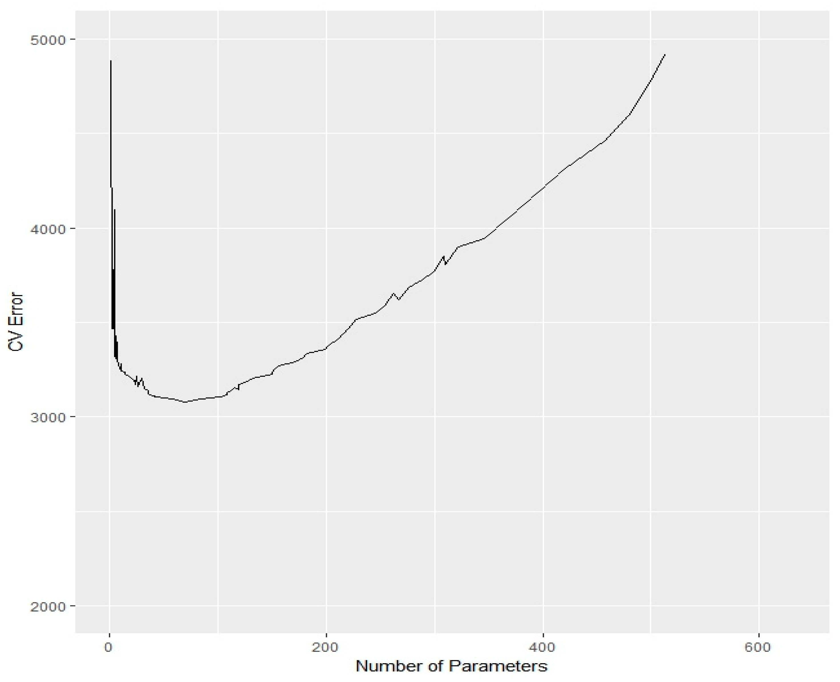
One possible form of calibration (e.g., McGuire et al. (2018)) proceeds as follows. A sequence of models is examined with increasing , and therefore with the number of covariates decreasing. The models with small tend to be over-parameterised, leading to poor predictive performance; those with large tend to be under-parameterised, again leading to poor predictive performance. The optimal model is chosen to minimise CV error.
It is evident that, by the nature of this calibration, the lasso will be expected to lead to high forecast efficiency.
Figure 3 provides a numerical example of the variation of CV error with the number of parameters used to model a particular data set.
The lasso is a relatively recent addition to the actuarial literature, but a number of applications have already been made. Li et al. (2017) and Venter and Şahın (2018) used it to model mortality. Gao and Meng (2018) constructed a loss reserving lasso, modelling a 10 × 10 aggregate claim triangle and using a model broadly related to the chain ladder. McGuire et al. (2018) also constructed a loss reserving lasso, but modelling a large data set of individual claims containing a number of complex data features, some of which will be described in Section 6.
5.3. Granular (or Micro-) Models
Granular models, sometimes referred to as micro-models, are not especially well-defined. The general idea is that they endeavour to extend modelling into some of the detail that underlies the aggregate data in a claim triangle. For example, a granular model may endeavour to model individual claims in terms of the detail of the claim process.
Hachemeister’s (1978, 1980) individual claim model has already been mentioned. The early statistical case estimation models used in industry were also granular. See, for example, Taylor and Campbell (2002) for a model of workers compensation claims in which claimants move between “active” and “incapacitated” states, receiving benefits for incapacity and other associated benefits, such as medical costs.
The history of granular models is generally regarded as having commenced with the papers of Norberg (1993, 1999) and Hesselager (1994). These authors represented individual claims by a model that tracked a claim process through a sequence of key dates, namely accident date, notification date, partial payment date, …, partial payment date, final payment date, and closure date. The process is a marked process in the sense that each payment date is tagged with a payment amount (or mark).
This type of model has been implemented by Pigeon et al. (2013, 2014) and Antonio and Plat (2014). Comment will be made on the performance of these models in Section 8.2.
Distinction is sometimes made between aggregate and granular models, but it is debatable. The literature contains models with more extensive data inputs than just claim payment triangles. For example, the payment triangle might be supplemented by a claim count triangle, as in the Payments per Claim Incurred model described in Taylor (2000), or in the Double Chain Ladder of Miranda et al. (2013).
These models certainly use more extensive data than a simple claim amount triangle, but the data are still aggregated. It is more appropriate to regard claim models as forming a spectrum that varies from a small amount of conditioning data at one end (e.g., a chain ladder) to a very large amount at the other (e.g., the individual claim models of Pigeon, Antonio and Denuit).
6. The Anthropocene—Intelligent Beings Intervene
6.1. Artificial Neural Networks in General
By implication, the present section will be concerned with the application of machine learning (ML) to loss reserving. Once again, the classification of specific models as MLMs or not may be ambiguous. If ML is regarded as algorithmic investigation of patterns and structure in data with minimal human intervention, then the lasso of Section 5.2 might be regarded as an MLM.
There are other contenders, such as regression trees, random forests, support vector machines, and clustering (Wüthrich and Buser 2017), but the form of ML that has found greatest application to loss reserving is the artificial neural network (ANN), and this section will concentrate on these.
Just a brief word on the architecture of a (feed-forward) ANN, since it will be relevant to the discussion in Section 8.3. Using the notation of Kuo (2018), let the ANN input be a vector . Suppose there are () hidden layers of neurons, each layer a vector, with values denoted by ; a vector output layer, with a value denoted by ; and a vector prediction of some target quantity . Let the components of be denoted by .
The relevant computational relations are
where is a vector with components , the are prescribed activation functions, the are called activations, is a vector of weights, and is a vector of biases. The weights and biases are selected by the ANN to maximise the accuracy of the prediction.
The hidden layers need not be of equal length. The activation functions will usually be nonlinear.
An early application of an ANN was given by Mulquiney (2006), who modelled an earlier version of the data set used by McGuire et al. (2018) in Section 5.2. This consisted of a unit record file in respect of about 60,000 Auto Bodily Injury finalised claims, each tagged with its accident quarter, development quarter of finalisation, calendar quarter of finalisation, OT at finalisation and season of finalisation (quarter).
Prior GLM analysis of the data set over an extended period had been carried out by Taylor and McGuire (2004), as described in Section 4, and they found that claim costs were affected in a complex manner by the factors listed there. The ANN was able to identify these effects. For example, it identified:
- an accident quarter effect corresponding to the legislative change that occurred in the midst of the data; and
- SI that varied with both finalisation quarter and OT.
Although the ANN and GLM produced similar models, the ANN’s goodness-of-fit was somewhat superior to that of the GLM.
Interest in and experimentation with ANNs has accelerated in recent years. Harej et al. (2017) reported on an International Actuarial Association Working Group on individual claim development with machine learning. Their model was a somewhat “under-powered” ANN that assumed separate chain ladder models for paid and incurred costs, respectively, for individual claims, and simply estimated the age-to-age factors.
However, since both paid and incurred amounts were included as input information in both models, they managed to differentiate age-to-age factors for different claims, e.g., claims with small amounts paid but large amounts incurred showed higher development of payments.
A follow-up study, with a similar restriction of ANN form, namely pre-supposed chain ladder structure, was published by Jamal et al. (2018).
Kuo (2018) carried out reserving with deep learning ANN, i.e., with multiple hidden layers. In this case, no model structure was pre-supposed. The ANN was applied to 200 claim triangles (50 insurers, each four lines of business) by Meyers and Shi (2011), and its results compared with those generated by five other models, including chain ladder and several from Meyers (2015).
The ANN out-performed all contenders most of the time and, in other cases, was only slightly inferior to them. This is an encouraging demonstration of the power of the ANN, but the small triangles of aggregate data do not exploit the potential of the ANN, which can be expected to perform well on large data sets that conceal complex structures.
6.2. The Interpretability Problem
GMs and MLMs can greatly improve modelling power in cases of data containing complex patterns. GMs can delve deeply into the data and provide valuable detail of the claim process. Their formulation can, however, be subject to great, even unsurmountable, difficulties. MLMs, on the other hand, for the large part provide little understanding, but may be able to bypass the difficulties encountered by GMs. They may also be cost-effective in shifting modelling effort from the actuary to the algorithm (e.g., lasso).
MLMs’ greatest obstacle to useful implementation is the interpretability problem. Some recent applications of ANNs have sought to address this. For example, Vaughan et al. (2018) introduce their explainable neural network (xNN), in which the ANN architecture (8) to (10) is restricted in such a way that
for scalar constants μ, γ1, …, γK, vector constants β1, …, βK, and real-valued functions .
This formulation is an attempt to bring known structure to the prediction . It is similar to the use of basis functions in the lasso implementation of McGuire et al. (2018). The use of xNNs is as yet in its infancy but offers promise.
7. Model Assessment
The assessment of a specific loss reserving model needs to consider two main factors:
- the model’s predictive efficiency; and
- its fitness for purpose.
7.1. Adaptation of Species—Evolutionary Models
Let denote the quantum of total liability represented by the loss reserve, and the statistical estimate of it. Both quantities are viewed as random variables, and the forecast error is , also a random variable.
Loss reserving requires some knowledge of the statistical properties of . Obviously, the mean is required as the central estimate. Depending on the purpose of the reserving exercise, one may also require certain quantiles of for the establishment of risk margins and/or capital margins, but an important statistic will be the estimate of forecast error.
One such estimate is the mean square error of prediction (MSEP), defined as
The smaller the MSEP, the greater the predictive efficiency of , so a reasonable choice of model would often be that which minimises the MSEP (maximises prediction efficiency). As long as one is not concerned with quantiles other than moderate, e.g., 75%, this conclusion will hold. If there is a major focus on extreme quantiles, e.g., 99%, the criterion for model selection might shift to the tail properties of the distribution of .
It may often be assumed that is unbiased, i.e., , but (11) may remain a reasonable measure of forecast error in the absence of this condition.
The structure of MSEP is discussed at some length in Taylor (2000, sec. 6.6) and Taylor and McGuire (2016, chp. 4). Suffice to say here that it consists of three additive components, identified as:
- parameter error;
- process error; and
- model error.
As discussed in the cited references, model error is often problematic and, for the purpose of the present subsection, MSEP will be taken to be the sum of just parameter and process errors.
In one or two cases, MSEP may be obtained analytically, most notably in the case of the Mack model, as set out in detail in Mack (1993). The MSEP of a GLM forecast may be approximated by the delta method, discussed in Taylor and McGuire (2016, sec. 5.2).
However, generally, for non-approximative estimates, two methods are available, namely:
- the bootstrap (Taylor and McGuire 2016, sec. 5.3); and
- (in the case of Bayesian models) Markov Chain Monte Carlo (MCMC) (Meyers 2015).
7.2. Fitness for Purpose
In certain circumstances, forecasts of ultimate claim cost may be required at an individual level. Suppose, for example, a self-insurer adopts a system of devolving claim cost to cost centres, but has not the wherewithal to formulate physical estimates of those costs. Then, a GM or MLM at the level of individual claims will be required.
If a loss reserving model is required not only for the simple purpose of entering a loss reserve in a corporate account, but also to provide some understanding of the claims experience that might be helpful to operations, then a more elaborate model than the simplest, such as chain ladder, would be justified.
Such considerations will determine the subset of all available models that are fit for purpose. Within this subset, one would, in principle, still usually choose that with the maximum predictive efficiency.
8. Predictive Efficiency
The purpose of the present section is to consider the predictive efficiency of GMs and MLMs. It will be helpful to preface this discussion with a discussion of cascaded models.
8.1. Cascaded Models
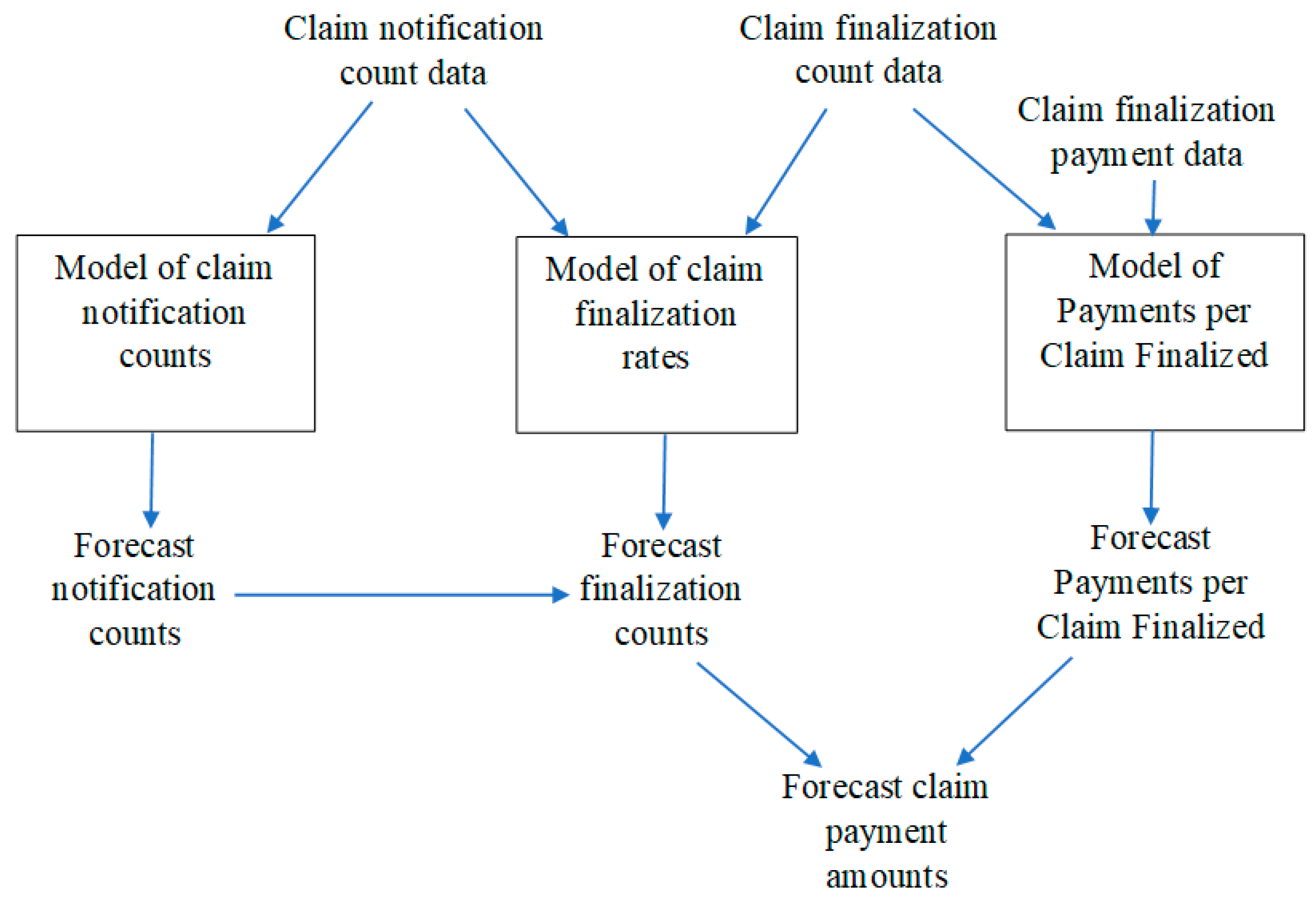
A cascaded model consists of a number of sub-models with the output of at least one of these providing input to another. An example is the Payments per Claim Finalized model discussed by Taylor (2000). This consists of three sub-models, as follows:
- claim notification counts;
- claim finalisation counts; and
- claim finalisation amounts.
The sub-models are configured as in Figure 4.
By contrast, the chain ladder consists of just a single model of claim amounts.
It is evident that increasing the number of sub-models within a model must add to the number of parameters, and it is well-known that, although too few parameters will lead to a poor model due to bias in forecasts, an increase in the number of parameters beyond a certain threshold will lead to poor predictive efficiency (over-parameterisation).
A cascaded model of sub-models would typically generate less biased forecasts than one of sub-models. However, the increased number of parameters might degrade predictive efficiency to the point where the more parsimonious model, even with its increased bias, is to be preferred.
It follows that the addition of a further sub-model will be justified only if the bias arising from its exclusion is sufficiently severe. This is illustrated in the empirical study by Taylor and Xu (2016) of many triangles from the data set of Meyers and Shi (2011).
They find that many of them are consistent with the assumptions of the chain ladder, in which case that model out-performs more elaborate cascaded models. However, there are also cases in which the chain ladder is a poor representation of the data, calling for a more elaborate model. In such cases, the cascaded models produce the superior performance.
8.2. Granular Models
The discussion of Section 8.1 perhaps sounds a cautionary note in relation to GMs. These are, by their nature, cascaded, e.g., a sub-model for the notification process, a sub-model for the partial payment process, etc. They may, in fact, be very elaborate, in which case the possibility of over-parameterisation becomes a concern.
A salutary remark in the consideration of GMs is that the (aggregate) chain ladder has minimum variance for over-dispersed Poisson observations (Taylor 2011). So, regardless of how one expands the scope of the input data (e.g., more precise accident and notification dates, individual claim data, etc.), the forecast of future claim counts will not be improved as long as the chain ladder assumptions are valid.
The GM literature is rather bereft of demonstration that a GM has out-performed less elaborate contenders. It is true that Huang et al. (2016) make this claim in relation to the data considered by them. However, a closer inspection reveals that their GM is essentially none other than the Payments per Claim Finalized model discussed in Section 8.1.
The model posits individual claim data, and generates individual claim loss reserves. However, the parameters controlling these individual reserves are not individual-claim-specific. So, the model appears to lie somewhere between an individual claim model and an aggregate model.
This does not appear to be a case of a GM producing predictive efficiency superior to that of an aggregate model. Rather, it is a case of a cascaded model producing efficiency superior to that of uncascaded models.
There is one other major characteristic of GMs that requires consideration. A couple of examples illustrate.
Example 1.
Recall Antonio and Plat (2014), whose model is of the type mentioned in Section 5.3, tracing individual claims through the process of occurrence, notification, partial payments and closure. Claim payments occur according to a distribution of delays from notification but, conditional on these, the severities of individual payments in respect of an individual claim are equi-distributed and stochastically independent.
In some lines of business, perhaps most but especially in Liability lines, this assumption will not withstand scrutiny. The payments of a medium-to-large claim typically tend to resemble the following profile: a series of relatively small payments (fees for incident reports, preliminary medical expenses), a payment of dominant size (settlement of agreed liability), followed possibly by a smaller final payment (completion of legal expenses).
Consequently, if a large payment (say $500 K) is made, the probability of another of anywhere near the same magnitude is remote. In other words, the model requires recognition of dependency between payments.
Example 2.
(From Taylor et al. (2008)). Consider a GM of development of case estimates over time. Suppose an estimate of ultimate liability in respect of an individual claim increases 10-fold, from $5 K to $50 K, over a particular period. Then, typically, the probability of a further 10-fold increase, from $50 K to $500 K, in the next period will be low.
The reason is that the first increase signifies the emergence of information critical to the quantum of the claim, and it is unusual that further information of the same importance would emerge separately in the following period. Again, the random variables describing the development of a claim cannot be assumed to be stochastically independent.
Taylor et al. (2008) suggest an estimation procedure that allows for any such dependency without the need for its explicit measurement.
The essential point to emerge from this discussion is that the detail of a claim process usually involves a number of intricate dependencies. One ignores these at one’s peril, but taking account of them may well be problematic, since it opens the way to a hideously complex model with many dependency parameters. This, in turn, raises the spectre of over-parameterisation, and its attendant degradation of predictive efficiency, not to mention possible difficulty in the estimation of the dependency parameters.
This by no means condemns GMs, but it appears to me that the jury is still out on them; they have yet to prove their case.
8.3. Artificial Neural Networks
ANNs are effective tools for taking account of obscure or complex data structures. Recall the data set used by Mulquiney’s (2006) ANN in Section 6, which had been previously modelled with a GLM. It is evident from the description of the results that the GLM would have required a number of interactions:
- for the legislative effect, interaction between accident quarter and OT;
- for SI, interaction between finalisation quarter and OT.
The seeking out of such effects in GLM modelling (feature selection) can be difficult, time-consuming and expensive. This point is made by McGuire et al. (2018) in favour of the lasso, which is intended to automate feature selection.
The ANN is an alternative form of automation. As can be seen from the model form set out in (8) to (10), no explicit feature selection is attempted. The modelling is essentially an exercise in nonlinear curve-fitting, the nonlinearity arising from the activation functions. The number of parameters in the model can be controlled by cross-validation, as described in Section 5.2.
To some extent ANNs provide a rejoinder to the dependency issues raised in Section 8.2. Identification of dependencies becomes a mere special case of feature selection, and is captured obscurely by (8) to (10).
On the other hand, the abstract curve-fitting nature of ANNs renders them dangerously susceptible to extrapolation errors. Consider SI, for example. In the forecast of a loss reserve, one needs to make some assumption for the future. A GLM will have estimated past SI, and while this might not be blindly extrapolated into the future, it can provide valuable information, perhaps to be merged with collateral information, leading to a reasoned forecast.
In the case of an ANN, any past SI will have been “modelled” in the sense that the model may include one or more functions that vary over calendar quarter, but these curves may interact with other covariates, as mentioned above, and the extraction of all this information in an organised and comprehensible form may present difficulties. Mulquiney (2006) alludes to this issue.
All actuaries are familiar with text-book examples of curves (e.g., polynomials) that fit well to past data points, but produce wild extrapolations into the future. Blind extrapolation of ANNs can, on occasion, produce such howlers. Suffice to say that care and, possibly, skill is required in their use for forecasting.
9. The Watchmaker and the Oracle
The tendency of GMs (watchmaking) is to increase the number of cascaded models (relative to aggregate models), first to individual claim modelling, then perhaps to individual transaction modelling, to dissect the available data in ever greater detail, to increase the number of model components and the complexity of their connections, and then assemble an integrated model from all the tiny parts.
If this can be achieved, it will provide powerful understanding of the claim process in question. However, as indicated in Section 8.2, the process is fraught with difficulty. The final model may be over-simplified and over-parameterised, with unfavourable implications for predictive efficiency. In addition, the issue of modelling complex stochastic dependencies may be difficult, or even impossible, to surmount.
One may even discover that all sub-models pass goodness-of-fit tests, and yet the integrated model, when assembled, does not. This can arise because of inappropriate connections between the sub-models or overlooked dependencies.
An example of this can occur in the workers compensation framework mentioned in Section 5.3. One might successfully model persistence in the active state as a survival process, and persistence in the incapacitated state as a separate survival process, and then combine the two to forecast a worker’s future incapacity experience.
However, the active survival intensities may not be independent of the worker’s history. A claim recently recovered from incapacity may be less likely to return to it over the following few days than a worker who has never been incapacitated. Failure to allow for this dependency (and possibly other similar ones) will lead to unrealistic forecasts of future experience.
The behaviour of the ANN is Oracle-like. It is presented with a question. It surveys the available information, taking account of all its complexities, and delivers an answer, with little trace of reasoning.
It confers the benefit of bypassing many of the challenges of granular modelling, but the price to be paid for this is an opaque model. This is the interpretability problem. Individual data features remain hidden within the model. They may also be sometimes poorly measured without the human assistance given to more structured models. For example, diagonal effects might be inaccurately measured, but compensated for by measured, but actually nonexistent, row effects. Similar criticisms can be levelled at some other MLMs, e.g., lasso.
The ANN might be difficult to validate. Cross-validation might ensure a suitably small MSEP overall. However, if a poor fit is found in relation to some subset of the data, one’s recourse is unclear. The abstract nature of the model does not lend itself easily to spot-correction.
10. Conclusions
Aggregate models have a long track record. They are demonstrably adequate in some situations, and dubious to unsuitable in others. Cases may easily be identified in which a model as simple as the chain ladder works perfectly, and no other approach is likely to improve forecasting with respect to either bias or precision.
However, these simple models are characterised by very simple assumptions and, when a data set does not conform to these assumptions, the performance of the simple models may be seriously disrupted. Archetypal deviations from the simple model structures are the existence of variable SI, structural breaks in the sequence of average claim sizes over accident periods, or variable claim settlement rates (see e.g., Section 4).
When disturbances of this sort occur, great flexibility in model structure may be required. For a few decades, GLMs have provided this (see Section 4). GLMs continue to be applicable and useful. However, the fitting of these models requires considerable time and skill, and is therefore laborious and costly.
One possible response to this is the use of regularised regression, and the lasso in particular (Section 5.2). This latter model may be viewed as a form of MLM in that it automates model selection. This retains all the advantages of a GLM’s flexibility, but with the reduced time and cost of calibration flowing from automation, and also provides a powerful guard against over-parameterisation.
The GMs of Section 5.3 are not a competitor of the GLM. Rather, they attempt to deconstruct the claim process into a number of components and model each of these. GLMs may well be used for the component modelling.
This approach may extract valuable information about the claim process that would otherwise be unavailable. However, as pointed out in Section 8.2, there will often be considerable difficulty in modelling some dependencies in the data, and failure to do so may be calamitous for predictive accuracy.
Most GMs are also cascaded models and, indeed, some are extreme cases of these. Section 8.1 points out that the complexity of cascaded models, largely reflected in the number of sub-models, comes with a cost in terms of enlarged predictive error (MSEP). They are therefore useful only when the failure to consider sub-models would cause the introduction of prediction bias worse than the increase in prediction error caused by their inclusion.
The increased computing power of recent years has enabled the recruitment of larger data sets, with a greater number of explanatory variables for loss reserving, or lower-level, such as individual claim, data. This can create difficulties for GMs and GLMs. The greater volume of data may suggest greater model complexity. It may, for example, necessitate an increase in the number of sub-models within a GLM.
If a manually constructed GLM were to be used, the challenges of model design would be increased. It is true, as noted above, that these are mitigated by the use of a lasso (or possibly other regularisation), but not eliminated.
Automation of such a model requires a selection of the basis functions mentioned in Section 6.2. It is necessary that the choice allow for interactions of all orders to be recognised in the model. As the number of potential covariates if the model increases, the number of interactions can mount very rapidly, possibly to the point of unworkability. This will sometimes necessitate the selection of interaction basis functions by the modeler, at which point erosion of the benefits of automated model design begins.
ANNs endeavour to address this situation. Their very general structure (see (8) to (10)) renders them sufficiently flexible to fit a data set usually as well as a GLM, and to identify and model dependencies in the data. They represent the ultimate in automation, since the user has little opportunity to intervene in feature selection.
However, this flexibility comes at a price. The output function of the ANN, from which the model values are fitted to data points, becomes abstract and inscrutable. While providing a forecast, the ANN may provide the user with little or no understanding of the data. This can be dangerous, as the user may lack control over extrapolation into the future (outside the span of the data) required for prediction.
The literature contains some recent attempts to improve on this situation with xNNs, which endeavor to provide some shape for the network’s output function, and so render it physically meaningful. For example, the output function may be expressed in terms of basis functions parallel to those used for a lasso. However, experience with this form of lasso indicates that effort may still be required for interpretation of the model output expressed in this form.
In summary, the case is still to be made for both GMs and MLMs. Particular difficulties are embedded in GMs that may prove insurmountable. MLMs hold great promise but possibly require further development if they are to be fully domesticated and realise their loss-reserving potential.
A tantalising prospect is the combination of GMs and ANNs to yield the best of both worlds. To the author’s knowledge, no such model has yet been formulated, but the vision might be the definition of a cascaded GM with one or more ANNs used to fit the sub-models or the connections between them, or both.
Funding
This research was funded by the Australian Research Council’s Linkage Projects funding scheme, project number LP130100723.
Conflicts of Interest
The author declares no conflict of interest in the production of this research.
References
- Ahlgren, Marcus. 2018. Claims Reserving Using Gradient Boosting and Generalized Linear Models. Master’s thesis, KTH Royal Institute of Technology School of Engineering Sciences, Stockholm, Sweden. Available online: http://www.diva-portal.org/smash/record.jsf?pid=diva2%3A1215659&dswid=-4333 (accessed on 19 July 2019).
- Antonio, K., and R. Plat. 2014. Micro-level stochastic loss reserving for general insurance. Scandinavian Actuarial Journal 2014: 649–69. [Google Scholar] [CrossRef]
- Baxter, L. A., S. M. Coutts, and S. A. F. Ross. 1980. Applications of linear models in motor insurance. Transaction of the 21st International Congress of Actuaries 2: 11. [Google Scholar]
- Brockman, M. J., and T. S. Wright. 1992. Statistical motor rating: Making effective use of your data. Journal of the Institute of Actuaries 119: 457–526. [Google Scholar] [CrossRef]
- Fisher, W. H., and J. T. Lange. 1973. Loss reserve testing: A report year approach. Proceedings of the Casualty Actuarial Society 60: 189–207. [Google Scholar]
- Gabrielli, A. 2019. A Neural Network Boosted Double OverDispersed Poisson Claims Reserving Model. Available online: https://ssrn.com/abstract=3365517 (accessed on 19 July 2019).
- Gao, G., and S. Meng. 2018. Stochastic claims reserving via a Bayesian spline model with random loss ratio effects. ASTIN Bulletin 48: 55–88. [Google Scholar] [CrossRef]
- Hachemeister, C. A. 1978. A structural model for the analysis of loss reserves. Bulletin d’Association Royal des Actuaires Belges 73: 17–27. [Google Scholar]
- Hachemeister, C. A. 1980. A stochastic model for loss reserving. Transactions of the 21st International Congress of Actuaries 1: 185–94. [Google Scholar]
- Hachemeister, C. A., and J. N. Stanard. 1975. IBNR Claims Count Estimation with Static Lag Functions. Arlington County: Casualty Actuarial Society. [Google Scholar]
- Harej, B., R. Gächter, and S. Jamal. 2017. Individual Claim Development with Machine Learning. Report of the ASTIN Working Party of the International Actuarial Association. Available online: http://www.actuaries.org/ASTIN/Documents/ASTIN_ICDML_WP_Report_final.pdf (accessed on 19 July 2019).
- Harvey, A. C. 1989. Forecasting, Structural Time Series and the Kalman Filter. Cambridge: Cambridge University Press. [Google Scholar]
- Hesselager, O. 1994. A Markov Model for Loss Reserving. Astin Bulletin 24: 183–93. [Google Scholar] [CrossRef]
- Huang, J., X. Wu, and X. Zhou. 2016. Asymptotic behaviors of stochastic reserving: Aggregate versus individual models. European Journal of Operational Research 249: 657–66. [Google Scholar] [CrossRef]
- Jamal, S., S. Canto, R. Fernwood, C. Giancaterino, M. Hiabu, L. Invernizzi, T. Korzhynska, Z. Martin, and H. Shen. 2018. Machine Learning & Traditional Methods Synergy in Non-Life Reserving. Report of the ASTIN Working Party of the International Actuarial Association. Available online: https://www.actuaries.org/IAA/Documents/ASTIN/ASTIN_MLTMS%20Report_SJAMAL.pdf (accessed on 19 July 2019).
- Kuo, K. 2018. DeepTriangle: A deep learning approach to loss reserving. arXiv arXiv:1804.09253v1. [Google Scholar]
- Li, H., C. O’Hare, and F. Vahid. 2017. A flexible functional form approach to mortality modeling: Do we need additional cohort dummies? Journal of Forecasting 36: 357–67. [Google Scholar] [CrossRef]
- McCullagh, P., and J. A. Nelder. 1989. Generalized Linear Models, 2nd ed. London: Chapman & Hall. [Google Scholar]
- McGuire, G., G. Taylor, and H. Miller. 2018. Self-Assembling Insurance Claim Models Using Regularized Regression and Machine Learning. Available online: https://papers.ssrn.com/sol3/papers.cfm?abstract_id=3241906 (accessed on 19 July 2019).
- Mack, T. 1993. Distribution-free calculation of the standard error of chain ladder reserve estimates. ASTIN Bulletin 23: 213–25. [Google Scholar] [CrossRef]
- Miranda, M. D., J. P. Nielsen, and R. J. Verrall. 2013. Double chain ladder. Astin Bulletin 42: 59–76. [Google Scholar]
- Meyers, G. G. 2015. Stochastic Loss Reserving Using Bayesian MCMC Models. CAS Monograph Series Number 1. Monograph Commissioned by the Casualty Actuarial Society; Arlington: Casualty Actuarial Society. [Google Scholar]
- Meyers, G. G., and P. Shi. 2011. Loss Reserving Data Pulled from NAIC Schedule P. Available online: http://www.casact.org/research/index.cfm?fa=loss_reserves_data (accessed on 19 July 2019).
- Mulquiney, P. 2006. Artificial Neural Networks in Insurance Loss Reserving. Paper Presented at the 9th Joint Conference on Information Sciences 2006—Proceedings, Kaohsiung, Taiwan, 8–11 October; Amsterdam: Atlantis Press. Available online: https://www.atlantis-press.com/search?q=mulquiney (accessed on 19 July 2019).[Green Version]
- Nelder, J. A., and R. W. M. Wedderburn. 1972. Generalised linear models. Journal of the Royal Statistical Society, Series A 135: 370–84. [Google Scholar] [CrossRef]
- Norberg, R. 1993. Prediction of outstanding liabilities in non-life insurance. Astin Bulletin 23: 95–115. [Google Scholar] [CrossRef]
- Norberg, R. 1999. Prediction of outstanding liabilities II. Model extensions variations and extensions. Astin Bulletin 29: 5–25. [Google Scholar] [CrossRef]
- Pigeon, M., K. Antonio, and M. Denuit. 2013. Individual loss reserving with the multivariate skew normal framework. Astin Bulletin 43: 399–428. [Google Scholar] [CrossRef]
- Pigeon, M., K. Antonio, and M. Denuit. 2014. Individual loss reserving using paid–incurred data. Insurance: Mathematics and Economics 58: 121–31. [Google Scholar]
- Reid, D. H. 1978. Claim reserves in general insurance. Journal of the Institute of Actuaries 105: 211–96. [Google Scholar] [CrossRef]
- Taylor, G. 2000. Loss Reserving: An Actuarial Perspective. Dordrecht: Kluwer Academic Publishers. [Google Scholar]
- Taylor, G. 2008. Second order Bayesian revision of a generalised linear model. Scandinavian Actuarial Journal 2008: 202–42. [Google Scholar] [CrossRef]
- Taylor, G. 2011. Maximum likelihood and estimation efficiency of the chain ladder. ASTIN Bulletin 41: 131–55. [Google Scholar]
- Taylor, G. C. 1986. Claims Reserving in Non-Life Insurance. Amsterdam: North-Holland. [Google Scholar]
- Taylor, G., and M. Campbell. 2002. Statistical Case Estimation. Research Paper No. 104 of the Centre for Actuarial Studies. University of Melbourne. Available online: https://fbe.unimelb.edu.au/__data/assets/pdf_file/0009/2592072/104.pdf (accessed on 19 July 2019).
- Taylor, G., and G. McGuire. 2004. Loss reserving with GLMs: A case study. Paper presented at the Spring 2004 Meeting of the Casualty Actuarial Society, Colorado Springs, CO, USA, May 16–19; pp. 327–92. [Google Scholar]
- Taylor, G., and G. McGuire. 2009. Adaptive reserving using Bayesian revision for the exponential dispersion family. Variance 3: 105–30. [Google Scholar]
- Taylor, G., and G. McGuire. 2016. Stochastic Loss Reserving Using Generalized Linear Models. CAS Monograph Series, Number 3, Monograph Commissioned by the Casualty Actuarial Society; Arlington: Casualty Actuarial Society. [Google Scholar]
- Taylor, G., G. McGuire, and J. Sullivan. 2008. Individual claim loss reserving conditioned by case estimates. Annals of Actuarial Science 3: 215–56. [Google Scholar] [CrossRef]
- Taylor, G., and P. Mulquiney. 2007. Modelling mortgage insurance as a multi-state process. Variance 1: 81–102. [Google Scholar]
- Taylor, G., and J. Xu. 2016. An empirical investigation of the value of finalisation count information to loss reserving. Variance 10: 75–120. [Google Scholar] [CrossRef]
- Tibshirani, R. 1996. Regression Shrinkage and Selection via the lasso. Journal of the Royal Statistical Society, Series B (Methodological) 58: 267–88. [Google Scholar] [CrossRef]
- Tweedie, M. C. K. 1984. An index which distinguishes between some important exponential families. In Statistics: Applications and New Directions, Proceedings of the Indian Statistical Golden Jubilee International Conference. Edited by J. K. Ghosh and J. Roy. West Bengal: Indian Statistical Institute, pp. 579–604. [Google Scholar]
- Vaughan, J., A. Sudjianto, E. Brahimi, J. Chen, and V. N. Nair. 2018. Explainable neural networks based on additive index models. arXiv arXiv:1806.01933v1. [Google Scholar]
- Venter, G. G., and Ş. Şahın. 2018. Parsimonious parameterization of age-period-cohort models by Bayesian shrinkage. ASTIN Bulletin 48: 89–110. [Google Scholar] [CrossRef]
- Wright, T. S. 1990. A stochastic method for claims reserving in general insurance. Journal of the Institute of Actuaries 117: 677–731. [Google Scholar] [CrossRef]
- Wüthrich, M. V. 2018a. Neural networks applied to chain-ladder reserving. European Actuarial Journal 8: 407–36. [Google Scholar] [CrossRef]
- Wüthrich, M. V. 2018b. Machine learning in individual claims reserving. Scandinavian Actuarial Journal 2018: 465–80. [Google Scholar] [CrossRef]
- Wüthrich, M. V., and C. Buser. 2017. Data Analytics for Non-Life Insurance Pricing. Zurich: RiskLab Switzerland, Department of Mathematics, ETH Zurich. [Google Scholar]
- Wüthrich, M. V., and M. Merz. 2008. Stochastic Claim Reserving Methods in Insurance. Chichester: John Wiley & Sons, Ltd. [Google Scholar]
Figure 1.
Illustration of the data triangle.

Figure 2.
Illustration of a forecast by age-to-age factors.

Figure 3.
An example of cross-validation error.

Figure 4.
The Payments per Claim Finalized model and its sub-models.


Table 1.
Special cases of regularised regression.
| Special Case | ||
|---|---|---|
| 0 | - | GLM |
| >0 | 1 | Lasso |
| >0 | 2 | Ridge regression |
© 2019 by the author. Licensee MDPI, Basel, Switzerland. This article is an open access article distributed under the terms and conditions of the Creative Commons Attribution (CC BY) license (http://creativecommons.org/licenses/by/4.0/).
Share and Cite
MDPI and ACS Style
Taylor, G. Loss Reserving Models: Granular and Machine Learning Forms. Risks 2019, 7, 82. https://0-doi-org.brum.beds.ac.uk/10.3390/risks7030082
AMA Style
Taylor G. Loss Reserving Models: Granular and Machine Learning Forms. Risks. 2019; 7(3):82. https://0-doi-org.brum.beds.ac.uk/10.3390/risks7030082
Chicago/Turabian StyleTaylor, Greg. 2019. "Loss Reserving Models: Granular and Machine Learning Forms" Risks 7, no. 3: 82. https://0-doi-org.brum.beds.ac.uk/10.3390/risks7030082
Note that from the first issue of 2016, this journal uses article numbers instead of page numbers. See further details here.