Machine Learning in Least-Squares Monte Carlo Proxy Modeling of Life Insurance Companies


1
Department of Mathematics, TU Kaiserslautern, Erwin-Schrödinger-Straße, Geb. 48, 67653 Kaiserslautern, Germany
2
Mathematical Institute, University Cologne, Weyertal 86-90, 50931 Cologne, Germany
3
Department Financial Mathematics, Fraunhofer ITWM, Fraunhofer-Platz 1, 67663 Kaiserslautern, Germany
*
Author to whom correspondence should be addressed.
Risks 2020, 8(1), 21; https://0-doi-org.brum.beds.ac.uk/10.3390/risks8010021
Submission received: 30 December 2019
/
Revised: 10 February 2020
/
Accepted: 12 February 2020
/
Published: 21 February 2020
(This article belongs to the Special Issue Machine Learning in Insurance)
Abstract
:Under the Solvency II regime, life insurance companies are asked to derive their solvency capital requirements from the full loss distributions over the coming year. Since the industry is currently far from being endowed with sufficient computational capacities to fully simulate these distributions, the insurers have to rely on suitable approximation techniques such as the least-squares Monte Carlo (LSMC) method. The key idea of LSMC is to run only a few wisely selected simulations and to process their output further to obtain a risk-dependent proxy function of the loss. In this paper, we present and analyze various adaptive machine learning approaches that can take over the proxy modeling task. The studied approaches range from ordinary and generalized least-squares regression variants over generalized linear model (GLM) and generalized additive model (GAM) methods to multivariate adaptive regression splines (MARS) and kernel regression routines. We justify the combinability of their regression ingredients in a theoretical discourse. Further, we illustrate the approaches in slightly disguised real-world experiments and perform comprehensive out-of-sample tests.
1. Introduction
The Solvency II directive of the European Parliament and European Council (2009) requires from insurance companies a derivation of the solvency capital requirement (SCR) using the full probability distributions of losses over a one-year period. Some life insurers comply with this requirement by setting up internal models. Other insurers opt for the much simpler standard formula, which enables an aggregation of the company’s exposures to single risks. Lacking an analytical valuation formula for the losses in a one-year period, life insurers with an internal model are supposed to utilize a Monte Carlo approach usually called nested simulations approach (Bauer et al. (2012)). In practice their cash-flow-projection (CFP) models need to be simulated several hundred thousand to several million times for a robust implementation of the nested simulations approach. But the insurers are currently far from being endowed with sufficient computational capacities to perform such expensive simulation tasks. By applying suitable approximation techniques like the least-squares Monte Carlo (LSMC) approach of Bauer and Ha (2015), the insurers are able to overcome these computational hurdles though. For example, they can implement the LSMC framework formalized by Krah et al. (2018) and applied by, for example, Bettels et al. (2014), to derive their full loss distributions. The central idea of this framework is to carry out a comparably small number of wisely chosen nested Monte Carlo simulations and to feed the simulation results into a supervised machine learning algorithm that translates the results into a proxy function of the insurer’s loss (output) with respect to the underlying risk factors (input).
Our starting point is the LSMC framework from Krah et al. (2018). In the following the same approach for the proxy derivation is assumed, we will only amend the calibration and validation steps. Therefore, we neither repeat the simulation setting nor the procedure for the full loss distribution forecast and SCR calculation here in detail. The purpose of this exposition is to introduce different machine learning methods that can be applied in the calibration step of the LSMC framework, to point out their similarities and differences and to compare their out-of-sample performances in the same slightly disguised real-world LSMC example already used in Krah et al. (2018).
We describe the data basis used for calibration and validation in Section 2.1, the structure of the calibration algorithm in Section 2.2 and our validation approach in Section 2.3. Our focus lies on out-of-sample performance rather than computational efficiency as the latter becomes only relevant if the former gives reason for it. We analyze a very realistic data basis with 15 risk factors and validate the proxy functions based on a very comprehensive and computationally expensive nested simulations test set comprising the SCR estimate.
The main idea of our approach is to combine different regression methods with an adaptive algorithm, in which the proxy functions are built up of basis functions in a stepwise fashion. In a four risk factor LSMC example, Teuguia et al. (2014) applied a full model approach, forward selection, backward elimination and a bidirectional approach as, for example, discussed in Hocking (1976) with orthogonal polynomial basis functions. They stated that only forward selection and the bidirectional approach were feasible when the number of risk factors or the polynomial degree exceeded 7, as then the resulting other models exploded. Life insurance companies covering a wide range of contracts in their portfolio are typically exposed to even more risk factors like, for example, 15. Complex business regulation frameworks such as those in Germany cause non-linear dependencies between risk factors and losses, which naturally lead to polynomials of higher degrees in the chosen proxy models. In these cases, even the standard forward selection and bidirectional approaches become infeasible as the sets of candidate terms from which the basis functions are chosen will explode then as well. We therefore follow the suggestion of Krah et al. (2018) to implement the so-called principle of marginality, an iteration-wise update technique of the set of candidate terms that lets the algorithm get along with comparably few carefully selected candidate terms.
Our main contribution is to identify, explain and illustrate a collection of regression methods and model selection criteria from the variety of regression design options that provide suitable proxy functions in the LSMC framework when applied in combination with the principle of marginality. After some general remarks in Section 3.1, we describe ordinary least-squares (OLS) regression in Section 3.2, generalized linear models (GLMs) by Nelder and Wedderburn (1972) in Section 3.3, generalized additive models (GAMs) by Hastie and Tibshirani (1986) and Hastie and Tibshirani (1990) in Section 3.4, feasible generalized least-squares (FGLS) regression in Section 3.5, multivariate adaptive regression splines (MARS) by Friedman (1991) in Section 3.6, and kernel regression by Watson (1964) and Nadaraya (1964) in Section 3.7. While some regression methods such as OLS and FGLS regression or GLMs can immediately be applied in conjunction with numerous model selection criteria such as Akaike information criterion (AIC), Bayesian information criterion (BIC), Mallow’s or generalized cross-validation (GCV), other regression methods such as GAMs, MARS, kernel, ridge or robust regression require well thought-through modifications thereof or work only with non-parametric alternatives such as k-fold or leave-one-out cross-validation. For adaptive approaches of FGLS, ridge and robust regression in life insurance proxy modeling, see also Hartmann (2015), Krah (2015) and Nikolić et al. (2017), respectively.
In the theory sections, we present the models with their assumptions, important properties and popular estimation algorithms and demonstrate how they can be embedded in the adaptive algorithm by proposing feasible implementation designs and combinable model selection criteria. While we shed light on the theoretical basic concepts of the models to lay the groundwork for the application and interpretation of the later following numerical experiments, we forego describing in detail technical enhancements or peculiarities of the involved algorithms and instead refer the interested reader to further sources. Additionally we provide the practicioners with R packages containing useful implementations of the presented regression routines. We complement the theory sections by corresponding empirical results in Section 4, throughout which we perform the same Monte Carlo approximation task to make the performance of the various methods comparable. We measure the approximation quality of the resulting proxy functions by means of aggregated validation figures on three out-of-sample test sets.
Conceivable alternatives to the entire adaptive algorithm are other typical machine learning techniques such as artificial neural networks (ANNs), decision tree learning or support vector machines. In particular, the classical feed forward networks proposed by Hejazi and Jackson (2017) and applied in various ways by Kopczyk (2018), Castellani et al. (2018), Born (2018) and Schelthoff (2019) were shown to capture the complex nature of CFP models well. A major challenge here is not only to find reliable hyperparameters such as the numbers of hidden layers and nodes in the network, batch size, weight initializer probability distribution, learning rate or activation functions but also the high dependence on the random seeds. We plan to contribute to this in a further publication which will be dedicated to hyperparameter search algorithms and stabilization methods such as ensemble methods. As an alternative to feed forward networks, Kazimov (2018) suggested to use radial basis function networks albeit so far none of the tested approaches performed better than the ordinary least squares regression in Krah et al. (2018).
In decision tree learning, random forests and tree-based gradient boosting machines were considered by Kopczyk (2018) and Schoenenwald (2019). While random forests were outperformed by feed forward networks but did better than the least absolute shrinkage and selection operator (LASSO) by Tibshirani (1996) in the example of the former author, they generally performed worse than the adaptive approaches by Krah et al. (2018) with OLS regression in numerous examples of the latter author. The gradient boosting machines, requiring more parameter tuning and thus being more versatile and demanding, came overall very close to the adaptive approaches.
Castellani et al. (2018) compared support vector regression (SVR) by Drucker et al. (1997) to ANNs and the adaptive approaches by Teuguia et al. (2014) in a seven risk factor example and found the performance of SVR placed somewhere inbetween the other two approaches with the ANNs getting closest to the nested simulations benchmark. As some further non-parametric approaches, Sell (2019) tested least-squares support-vector machines (LS-SVM) by Suykens and Vandewalle (1999) and shrunk additive least-squares approximations (SALSA) by Kandasamy and Yu (2016) in comparison to ANNs and the adaptive approaches by Krah et al. (2018) with OLS regression. In his examples, SALSA was able to beat the other two approaches whereas LS-SVM was left far behind. The analyzed machine learning alternatives have in common that they require at least to some degree a fine-tuning of some model hyperparameters. Since this is often a non-trivial but crucial task for generating suitable proxy functions, finding efficient and reliable search algorithms should become a subject of future research.
2. Calibration and Validation in the LSMC Framework
2.1. Fitting and Validation Points
2.1.1. Outer Scenarios and Inner Simulations
Our starting point is the LSMC approach (Krah et al. (2018)). LSMC proxy functions are calibrated conditional on the fitting points generated by the Monte Carlo simulations of the CFP model. Additional out-of-sample validation points serve as a mean for an assessment of the goodness-of-fit. The explaining variables of a proxy function are financial and actuarial risks the insurance company is exposed to. Examples for these risks are changes in interest rates, equity, credit, mortality, morbidity, lapse and expense levels over the one-year period. The dependent variable is an economic variable like the available capital, loss of available capital or best estimate of liabilites over the one-year period. Figure 1 plots the fitting values of an exemplary economic variable with respect to a financial risk factor. By an outer scenario we refer to a specific realized stress level combination of these risk factors over one year, and by an inner simulation to a stochastic path of an outer scenario in the CFP model under the given risk-neutral probability measure. Each outer scenario is assigned the probability weighted mean value of the economic variable over the corresponding inner simulations. In the LSMC context the fitting values are the mean values over only few inner simulations whereas the validation values are derived as the mean values over many inner simulations.
2.1.2. Different Trade-Off Requirements
According to the law of large numbers, this construction makes the validation values comparably stable while the fitting values are very volatile. Typically, the very limited fitting and validation simulation budgets are of similar sizes. Hence the few inner simulations in the case of the fitting points allow a great diversification among the outer scenarios whereas the many inner simulations in the case of the validation points let the validation values be quite close to their expectations but at the cost of only little diversification among the outer scenarios. These opposite ways to deal with the trade-off between the numbers of outer scenarios and inner simulations reflect the different requirements for the fitting and validation points in the LSMC approach. While the fitting scenarios should cover the domain of the real-world scenarios well to serve as a good regression basis, the validation values should approximate the expectations of the economic variable at the validation scenarios well to provide appropriate target values for the proxy functions.
2.2. Calibration Algorithm
2.2.1. Five Major Components
The calibration of the proxy function is performed by an adaptive algorithm that can be decomposed into the following five major components: (1) a set of allowed basis function types for the proxy function, (2) a regression method, (3) a model selection criterion, (4) a candidate term update principle, and (5) the number of steps per iteration and the directions of the algorithm. For illustration, we adopt the flowchart of the adaptive algorithm from Krah et al. (2018) and depict it in Figure 2. While components (1) and (5) enter the flowchart implicitly through the start proxy, candidate terms and the order of the processes and decisions in the chart, components (2), (3) and (4) are explicitly indicated through the labels “Regression”, “Model Selection Criterion” and “Get Candidate Terms”.
Let us briefly recapitulate the choice of components (1)–(5) from the successful applications of the adaptive algorithm in the insurance industry as described in Krah et al. (2018). As the function types for the basis functions (1), let only monomials be allowed. Let the regression method (2) be ordinary least-squares (OLS) regression and the model selection criterion (3) Akaike information criterion (AIC) from Akaike (1973). Let the set of candidate terms (4) be updated by the principle of marginality to which we will return in greater detail below. Lastly, when building up the proxy function iteratively, let the algorithm make only one step per iteration in the forward direction (5) meaning that in each iteration exactly one basis function is selected which cannot be removed anymore (adaptive forward stepwise selection).
2.2.2. Iterative Procedure
The algorithm starts in the upper left side of Figure 2 with the specification of the start proxy basis functions. We specify only the intercept so that the first regression () reduces to averaging over all fitting values. In order to harmonize the choices of OLS regression and AIC, we assume that the errors are normally distributed and homoscedastic because then the OLS estimator coincides with the maximum likelihood estimator. AIC is a relative measure for the goodness-of-fit of the proxy function and is defined as twice the negative of the maximum log-likelihood plus twice the number of degrees of freedom. The smaller the AIC score, the better the fit, and thus the trade-off between a too complex (overfitting) and too simple model (underfitting).
At the beginning of each iteration (), the set of candidate terms is updated by the principle of marginality which stipulates that a monomial basis function becomes a candidate if and only if all its derivatives are already included in the proxy function. The choice of a monomial basis is compatible to the principle of marginality. Using such a principle saves computational costs by selecting the basis functions conditionally on the current proxy function structure. In the first iteration (), all linear monomials of the risk factors become candidates as their derivatives are constant values which are represented by the intercept.
The algorithm proceeds on the lower left side of the flowchart with a loop in which all candidate terms are separately added to the proxy function structure and tested with regard to their additional explanatory power. With each candidate, the fitting values are regressed against the fitting scenarios and the AIC score is calculated. If no candidate reduces the currently smallest AIC score, the algorithm terminates, and otherwise, the proxy function is updated by the one which reduces AIC most. Then the next iteration () begins with the update of the set of candidate terms, and so on. As long as no termination occurs, this procedure is repeated until the prespecified maximum number of terms is reached.
2.3. Validation Figures
2.3.1. Validation Sets
Since it is the objective of this paper to propose suitable regression methods for the proxy function calibration in the LSMC framework, we introduce several validation figures serving as indicators for the approximation quality of the proxy functions. We measure the out-of-sample performance of each proxy function on three different validation sets by calculating five validation figures per set.
The three validation sets are a Sobol set, a nested simulations set and a capital region set. Unlike the Sobol set, the nested simulations and capital region sets do not serve as feasible validation sets in the LSMC routine as they become known only after evaluating the proxy function as explained below. Furthermore, they require massive computational capacities. Yet they can be regarded as the natural benchmark for the LSMC-based method and are thus very valuable for this analysis. Figure 3 plots the nested simulation values of an exemplary economic variable with respect to a financial risk factor. The Sobol set consists of, for example, between and Sobol validation points, of which the scenarios follow a Sobol sequence covering the fitting space uniformly. Thereby, the fitting space is the cube on which the outer fitting scenarios are defined. It has to cover the space of real-world scenarios used for the full loss distribution forecast sufficiently well. For interpretive reasons, sometimes the Sobol set is extended by points with, for example, one-dimensional risk scenarios or scenarios producing a risk capital close to the SCR ( value-at-risk) in previous risk capital calculations.
The nested simulations set comprises the, for example, to validation points of which the scenarios correspond to the, for example, highest to losses from the full loss distribution forecast made by the proxy function that had been derived under the standard calibration algorithm choices described in Section 2.2. Like in the example of Chapter 5.2 in Krah et al. (2018), the order of these losses-which scenarios lead to which quantiles?following from the fourth and last step of the LSMC approach is very similar to the order following from the nested simulations approach. Therefore the scenarios of the nested simulations set are simply chosen by the order of the losses resulting from the LSMC approach. Several of these scenarios consist of stresses falling out of the fitting space. Compare Figure 1 and Figure 3 which depict fitting and nested simulation values from the same proxy modeling task with respect to the same risk factor. Severe outliers due to extreme stresses far outside of the fitting space should be excluded from the set. The capital region set is a subset of the nested simulations set containing the nested simulations SCR estimate, that is, the scenario leading to the loss, and the, for example, 64 losses above and below, which makes in total, for example, validation points.
2.3.2. Validation Figures
The five validation figures reported in our numerical experiments comprise two normalized mean absolute errors (MAEs), one with respect to the magnitude of the economic variable itself and one with respect to the magnitude of the corresponding market value of assets. They comprise further the mean error, that is, the mean of the residuals, as well as two validation figures based on the change of the economic variable from its base value (see the definition of the base value below): the normalized MAE with respect to the magnitude of the changes and the mean error of these changes. The smaller the normalized MAEs are, the better the proxy function approximates the economic variable. However, the validation values are afflicted with Monte Carlo errors so that the normalized MAEs serve only as meaningful indicators as long as the proxy functions do not become too precise. The means of the residuals should be possibly close to zero since they indicate systematic deviations of the proxy functions from the validation values. While the first three validation figues measure how well the proxy function reflects the economic variable in the CFP model, the latter two address the approximation effects on the SCR, compare Chapter 3.4.1 of Krah et al. (2018).
Let us write the absolute value as and let L denote the number of validation points. Then we can express the MAE of the proxy function evaluated at the validation scenarios versus the validation values as . After normalizing the MAE with respect to the mean of the absolute values of the economic variable or the market value of assets, that is, with , we obtain the first two validation figures, that is,
In the following, we will refer to (1) with as the MAE with respect to the relative metric, and to (1) with as the MAE with respect to the asset metric. The mean of the residuals is given by
Let us refer by the base value to the validation value corresponding to the base scenario in which no risk factor has an effect on the economic variable. In analogy to (1) but only with respect to the relative metric, we introduce another normalized MAE by
The mean of the corresponding residuals is given by
3. Machine Learning Regression Methods
3.1. General Remarks
As the main part of our work, we will compare various types of machine learning regression approaches for determining suitable proxy functions in the LSMC framework. The methods we present in this section range from ordinary and generalized least-squares regression variants over GLM and GAM approaches to multivariate adaptive regression splines and kernel regression approaches.
The performance of the newly derived proxy functions when applied to the described validation sets is one way of comparing the different methods. Another way consists of ensuring compatibility with the principle of marginality and utilizing a suitable model selection criterion such as AIC in order to be able to compare iteration-wise the candidate models inside the approaches.
We will in the following sections shortly introduce the different methods, collect some theoretical properties and then concentrate on aspects of their implementation. Their numerical performance on the different validation sets is the subject of Section 4.
Our aim in the calibration step below is to estimate the conditional expectation under the risk-neutral measure given an outer scenario X. In contrast to Krah et al. (2018) does not necessarily have to be the available capital but can instead be, for example, the best estimate of liabilites or the market value of assets. The D-dimensional fitting scenarios are always generated under the physical probability measure on the fitting space which itself is a subspace of .
3.2. Ordinary Least-Squares (OLS) Regression
3.2.1. The Regression Model
In iteration of the adaptive forward stepwise algorithm (as given in Section 2.2), the OLS approximation consists of a linear combination of suitable linearly independent basis functions that is,
We call the predictor of or the systematic component.
With the fitting points and uncorrelated errors (the random components) having the same variance (= homoscedastic errors), we obtain the classical linear regression model
where and is the intercept. Then, the ordinary least-squares (OLS) estimator of the coefficients is given by
Using the notation the OLS problem is solved explicitly by
The proxy function for the economic variable given an outer scenario X is
For a practical implementation see, for example, function lm() in the R package stats of R Core Team (2018).
3.2.2. Gauss-Markov Theorem, ML Estimation and AIC
Under the assumptions of strict exogeneity (A1), a spherical error variance with the N-dimensional identity matrix (A2), and linearly independent basis functions (A3), we have (compare, for example, Hayashi (2000)):
- The OLS estimator is the best linear unbiased estimator (BLUE) of the coefficients in the classical linear regression model (7) (Gauss-Markov Theorem).
- If the errors in (7) are in addition normally distributed (A4), then the OLS estimator and the maximum likelihood (ML) estimator of the coefficients coincide.
- Under Assumptions (A1)-(A4) the Akaike information criterion (AIC) has the form
3.3. Generalized Linear Models (GLMs)
3.3.1. The Regression Model
The systematic component of a GLM (see Nelder and Wedderburn (1972) for its introduction) equals the linear predictor of the model in (6). However, one uses a monotonic link function that relates the economic variable to the linear predictor via
with .
Of course, the choice of the link function is a critical aspect. A possible motivation is a non-negativity requirement on that can be satisfied using . Further comments on choices of the link function are motivated below.
3.3.2. Canonical Link Function, GLM Estimation and IRLS Algorithm
While the normal distribution assumption for the random component allowed the derivation of nice properties in the linear model of the preceding section, the GLM considers random components with (conditional) distributions from the exponential family. Its canonical form with parameter is given by the density function
where , and are specific functions. For example, a normally distributed economic variable with mean and variance is given by , and with and .
For a random variable Y with a distribution from the exponential family, we have
is called a dispersion parameter, the variance function. We will in the following make the simplifying assumption , for a constant value of (A5) and then obtain the ML estimator in the GLM from Equation (13) as
Under (A5), there does in general not exist a closed-form solution for the GLM coefficient estimator (15). The resulting iterative method will be simplified for so-called canonical link functions which due to relation (14) are given by
with from the definition of the exponential family. Examples of pairs of canonical link functions and corresponding distributions are and the normal, and the gamma, and and the inverse Gaussian distribution.
In Chapter 2.5, McCullagh and Nelder (1989) apply Fisher’s scoring method to obtain an approximation to the GLM estimator. Further, McCullagh and Nelder (1989) justify how Fisher’s scoring method can be cast in the form of the iteratively reweighted least squares (IRLS) algorithm. To state the IRLS algorithm in our context, we need some notation.
Let be the estimate for the linear predictor evaluated at fitting scenario , compare (12). Let be the estimate for the economic variable, and the first derivative of the link function with respect to the economic variable evaluated at . Furthermore, we introduce the weight matrix with components given by
and the variance function from above evaluated at . Finally, we define with which allows us to formulate the IRLS algorithm for canonical link functions.
IRLS algorithm.
Perform the iterative approximation procedure below with an initialization of and as proposed by Dutang (2017) until convergence:
After convergence, we set .
Green (1984) proposes to solve the system which is equivalent to (18) via a QR decomposition to increase numerical stability. For a practical implementation of GLMs using the IRLS algorithm, see, for example, function glm() in R package stats of R Core Team (2018).
By inserting (17), (19) and the GLM estimator into (18) and by using (12), we obtain
that is, the GLM estimator minimizes the squared sum of raw residuals scaled by the estimated individual variances of the economic variable.
The Pearson residuals are defined as the raw residuals divided by the estimated individual standard deviations, that is,
3.3.3. AIC and Dispersion Estimation
Since AIC depends on the ML estimators, it is combinable with GLMs in the adaptive algorithm. Here, it has the form
where K is the number of coefficients and p indicates the number of the additional model parameters associated with the distribution of the random component. For instance, in the normal model, we have due to the error variance/dispersion. A typical estimate of the dispersion in GLMs is the Pearson residual chi-squared statistic divided by as described by Zuur et al. (2009) and implemented, for example, in function glm() belonging to R package stats, that is,
with given by (21). Even though this is not the ML estimator, it is a good estimate because, if the model is specified correctly, the Pearson residual chi-squared statistic divided by the dispersion is asymptotically distributed and the expected value of a chi-squared distribution with degrees of freedom is .
3.4. Generalized Additive Models (GAMs)
3.4.1. The Regression Model
Generalized additive models (GAMs) as introduced by Hastie and Tibshirani (1986) and Hastie and Tibshirani (1990) can be regarded as richly parameterized GLMs with smooth functions. While GAMs inherit from GLMs the random component (13) and the link function (12), they inherit from the additive models of Friedman and Stuetzle (1981) the linear predictor with the smooth functions. In the adaptive algorithm, we apply GAMs of the form
where , is the intercept and are the smooth functions to be estimated. In addition to the smooth functions, GAMs can also include simple linear terms of the basis functions as they appear in the linear predictor of GLMs. A smooth function can be written as a basis expansion
with coefficients and known basis functions which should not be confused with their arguments, namely the first-order basis functions . The slightly adapted Figure 4 from Wood (2006) depicts an exemplary approximation of y by a GAM with a basis expansion in one dimension without an intercept. The solid colorful curves represent the pure basis functions the dashed colorful curves show them after scaling with the coefficients and the black curve is their sum (25).
Typical examples for basis functions are thin plate regression splines, duchon splines, cubic regression splines or Eilers and Marx style P-splines. See, for example, function gam() in R package mgcv of Wood (2018) for a practical implementation of GAMs admitting these types of basis functions and using the PIRLS algorithm, which we present below.
3.4.2. Penalization and GAM Estimation via PIRLS Algorithm
Let the deviance corresponding to observation be where is independent of dispersion , where is the saturated log-likelihood and the log-likelihood. Then the model deviance can be written as . It is a generalization of the residual sum of squares for ML estimation. For instance, in the normal model the unit deviance is . For given smoothing parameters , the GAM estimator of the coefficients is defined as the minimizer of the penalized deviance
are the smoothing penalties. The smoothing parameters control the trade-off between a too wiggly model (overfitting) and a too smooth model (underfitting). The larger the values are, the more pronounced is the wiggliness of the basis functions reflected by their second derivatives in the minimization problem (27), and the higher is thus the penalty associated with the coefficients and the smoother is the estimated model.
A major advantage of the definition of GAMs via (24), (25), and (27) is its compatibility with information criteria and other model selection criteria such as generalized cross-validation. Besides, the resulting penalty matrix favors numerical stability in the PIRLS algorithm.
Since the saturated log-likelihood is a constant for a fixed distribution and set of fitting points, we can turn the minimization problem (27) into the maximization task of the penalized log-likelihood, that is,
Wood (2000) points out that Fisher’s scoring method can be cast in a penalized version of the iteratively reweighted least squares (PIRLS) algorithm when being used to approximate the GAM coefficient estimator (28). We formulate the PIRLS algorithm based on Marx and Eilers (1998) who indicate the iterative solution explicitly.
Let now be the GAM coefficient approximation in iteration t. Then the vector of the dependent variable and the weight matrix given by have the same form as in the IRLS algorithm, see (19) and (17). Additionally, let with belonging to the intercept be the penalty matrix.
PIRLS algorithm.
Perform the iterative approximation procedure below with initialization of and until convergence occurs:
After convergence, we set .
3.4.3. Smoothing Parameter Selection, AIC and Stagewise Selection
The smoothing parameters can be selected such that they minimize a suitable model selection criterion, for the sake of consistency, preferably the one used in the adaptive algorithm for basis function selection. The GAM estimator (28) does not exactly maximize the log-likelihood, therefore AIC has another form for GAMs than for GLMs. Hastie and Tibshirani (1990) propose a widely used version of AIC for GAMs, which uses effective degrees of freedom df in place of the number of coefficients . This is
where
Note that is already approximately calculated in the PIRLS algorithm. For GAMs, an estimate of the dispersion is obtained similarly to GLMs by (23). The parameter p is defined as in (22).
Another popular and effective smoothing parameter selection criterion invented by Craven and Wahba (1979) is generalized cross-validation (GCV), that is,
with the model deviance evaluated at the GAM estimator and the effective degrees of freedom defined just like for AIC.
Note that the adaptive forward stepwise algorithm depicted in Figure 2 can become computationally infeasible with GAMs as opposed to, for example, GLMs. In iteration k, a GAM has coefficients which need to be estimated while a GLM has only K coefficients. This difference in the estimation effort is increased further due to the iterative nature of the IRLS and PIRLS algorithms. Moreover, GAMs involve the task of optimal smoothing parameter selection. To deal with this aspect, Wood (2000), Wood et al. (2015) and Wood et al. (2017) have developed practical GAM fitting methods for large data sets. However, the suitable application of these methods in the adaptive algorithm is beyond the scope of our analysis, in particular as our focus is not on computational performance. Besides parallelizing the candidate loop on the lower left side of Figure 2, we achieve the necessary performance gains in GAMs by replacing the stepwise algorithm by a stagewise algorithm. This means that in each iteration, a predefined number L or proportion of candidate basis functions is selected simultaneously until a termination criterion is fulfilled. Thereby we select in one stage those basis functions which reduce the model selection criterion of our choice most when added separately to the current proxy function structure. When there are not at least as many basis functions as targeted, the algorithm shall be terminated after the ones which lead to a reduction in the model selection criterion have been selected.
3.5. Feasible Generalized Least-Squares (FGLS) Regression
3.5.1. The Regression Model
The regression model here equals the OLS case. However, we now let the errors have the covariance matrix where is positive definite and known and is unknown. We transform the generalized regression model according to Hayashi (2000) to obtain a model (*) which satisfies Assumptions (A1), (A2) and (A3) of the classical linear regression model. For this, choose an invertible matrix H with which can, for example, be the Cholesky matrix. Then, the generalized response vector , design matrix and error vector are given by
In analogy to the OLS estimator, the generalized least-squares (GLS) estimator of the coefficients is given as the minimizer of the generalized residual sum of squares, that is,
The closed-form expression of the GLS estimator is
and the proxy function becomes
where . The scalar can be estimated in analogy to OLS regression by where is the residual vector.
3.5.2. Gauss-Markov-Aitken Theorem and ML Estimation
Under the assumptions (A1), (A3), and a covariance matrix of which is positive definite and known (A6), we have:
- The GLS estimator is the BLUE of the coefficients in the generalized regression model (7) (Gauss-Markov-Aitken theorem).
- If in addition we have jointly normally distributed errors conditional on the fitting scenarios (A7) then the ML coefficient estimator coincides with the GLS estimator. Further, the ML estimator of the scalar can be expressed as times .
As a consequence, given a known matrix , we have a closed form solution for the GLS estimator that coincides with the ML estimator of the regression coefficients and the adaptive algorithm inside the LSMC approach goes through.
3.5.3. Unknown and FGLS Estimation via ML Algorithm
In the LSMC framework, is unknown. However, if a consistent estimator exists, we can apply feasible generalized least-squares (FGLS) regression, of which the estimator
has asymptotically the same properties as the GLS estimator (35).
With the FGLS proxy function is then given as
For the estimation of we will in the following set which can be done without loss of generality and consider . Furthermore, we assume in addition to (A1), (A3) and (A7) that the elements of the covariance matrix are twice differentiable functions of parameters with . We then write (A8). The following result is the basis of the iterative ML algorithm for the regression coefficients and the variance matrix.
Theorem 1.
The generalized regression model (7) under Assumptions (A1), (A3), (A7) and (A8) has the following first-order ML conditions:
where , and .
The system in (39) and (40) is then solved iteratively (see, for example, Magnus (1978)). We start the procedure with and then use PORT optimization routines as described in Gay (1990) and implemented in function nlminb() belonging to R package stats of R Core Team (2018). In this iterative routine, can be initialized, for example, by random numbers from the standard normal distribution.
ML algorithm.
Perform the following iterative approximation procedure with, for example, an initialization of until convergence:
- 1.
- Calculate the residual vector .
- 2.
- Substitute into the M equations in M unknowns given by (40) and solve them. If an explicit solution exists, set . Otherwise, select the maximum likelihood solution iteratively, for example, by using PORT optimization routines.
- 3.
- Calculate
Continue with the next iteration.
After convergence, we set and .
3.5.4. Heteroscedasticity, Variance Model Selection and AIC
Besides Assumption (A8) about the structure of the covariance matrix, we assume that the errors are uncorrelated with possibly different variances (= heteroscedastic errors), that is, . We model each variance , by a twice differentiable function in dependence of parameters and a suitable set of linearly independent basis functions , with , that is,
where is referred to as the variance function in analogy to for GLMs and GAMs. Without loss of generality, we set again .
Hartmann (2015) has already applied FGLS regression with different variance models in the LSMC framework. In her numerical examples, variance models with multiplicative heteroscedasticity led to the best performance of the proxy function in the validation. Therefore, we restrict our analyis on these kinds of structures, compare, for example, Harvey (1976), that is,
Like the proxy function, the variance function (43) has to be calibrated to apply FGLS regression, which means that the variance function has to be composed of suitable basis functions. Again, such a composition can be found with the aid of a model selection criterion. We still choose AIC, but have to take care for the fact that in FGLS regression the covariance matrix now contains M unknown parameters instead of only one in the OLS case (the same variance for all observations). Under Assumption (A7), AIC is given as
When using a variance model with multiplicative heteroscedasticity, AIC becomes
As an alternative or complement, the basis functions of the variance model can be selected with respect to their correlations with the final OLS residuals or based on graphical residual analysis.
For the final implementation of a variance model we use modified versions of two algorithms from Hartmann (2015). Our type I variant starts with the derivation of the proxy function by the standard adaptive OLS regression approach and then selects the variance model adaptively from the set of proxy basis functions of which the exponents sum up to at most two. The type II variant builds on the type I algorithm by taking the resulting variance model as given in its adaptive proxy basis function selection procedure with FGLS regression in each iteration.
Note further, that we should only apply FGLS regression as a substitute of OLS regression if heteroscedasticity prevails. This can be tested with the help of the Breusch-Pagan test of Breusch and Pagan (1979) for the following special structure of the variance function
where the function is twice differentiable and the first element of is . Further, the assumption of normally distributed errors is made. We use it in the numerical computations to check if heteroscedasticity still prevails during the iteration procedure.
3.6. Multivariate Adaptive Regression Splines (MARS)
3.6.1. The Regression Model
The multivariate adaptive regression splines (MARS) were introduced by Friedman (1991). The classical MARS model is a form of the classical linear regression model (7) where the basis functions are so-called hinge functions. Therefore, the theory of OLS regression applies in this context. GLMs (12) can also be applied in conjunction with MARS models. In this case we speak of generalized MARS models.
We describe the standard MARS algorithm in the LSMC routine according to Chapter 9.4 of Hastie et al. (2017). The building blocks of MARS proxy functions are reflected pairs of piecewise linear functions with knots t as depicted in Figure 5, that is,
where the , represent the risk factors that together form the outer scenario .
For each risk factor, reflected pairs with knots at each fitting scenario stress , are defined. All pairs are united in the following collection serving as the initial candidate basis function set of the MARS algorithm, that is,
We call the elements of hinge functions and consider them as functions over the entire input space . contains in total basis functions.
The adaptive basis function selection algorithm now consists of two parts, the forward and the backward pass.
3.6.2. Adaptive Forward Stepwise Selection and Forward Pass
The forward pass of the MARS algorithm can be viewed as a variation of the adaptive forward stepwise algorithm depicted in Figure 2. The start proxy function consists only of the intercept, that is, . In the classical MARS model, the regression method of choice is the standard OLS regression approach with the estimator (8), where in each iteration a reflected pair of hinge functions is selected instead of . Similarly, the regression method of choice in the generalized MARS model is the IRLS algorithm (18). Let us denote the MARS coefficient estimator by . Note that the theory on AIC cannot be transferred without any adjustments since the notion of the degrees of freedom has to be reconsidered due to the knots in the hinge functions acting as additional degrees of freedom.
After each iteration, the set of candidate basis functions is extended by the products of the last two selected hinge functions with all hinge functions in that depend on risk factors of which the last two selected hinge functions do not depend on. Let the reflected pair selected in the first iteration () be
Further, let . Then, the set of candidate basis functions is updated at the beginning of the second iteration () such that
The second set thus contains basis functions. Often, the order of interaction is limited to improve the interpretability of the proxy functions. Besides the maximum allowed number of terms, a minimum threshold for the decrease in the residual sum of squares can be employed as a termination criterion in the forward pass. Typically, the proxy functions generated in the forward pass overfit the data since model complexity is only penalized conservatively by stipulating a maximum number of basis functions and a minimum threshold.
3.6.3. Backward Pass and GCV
Due to the overfitting tendency of the proxy function generated in the forward pass, a backward pass is executed afterwards. Apart from the direction and slight differences, the backward pass is similar to the forward pass. In each iteration, the hinge function of which the removal causes the smallest increase in the residual sum of squares is removed and the backward model selection criterion for the resulting proxy function is evaluated. By this backward procedure, we generate the “best” proxy functions of each size in terms of the residual sum of squares. Out of all these best proxy functions, we finally select the one which minimizes the backward model selection criterion. As a result, the final proxy function will not only contain reflected pairs of hinge functions but also single hinge functions of which the complements have been removed. Optionally, the backward pass can also be omitted.
Let the number of basis functions in the MARS model be K and the number of knots be T. The standard choice for the backward model selection criterion is GCV defined as
with the effective degrees of freedom .
3.7. Kernel Regression
3.7.1. The One-dimensional Regression Model
Kernel regression (which goes back to Nadaraya (1964) and Watson (1964)) is a type of locally weighted OLS regression where the weights vary with the input variable (the target scenario). We start with locally constant (LC) regression where for each the fixed univariate kernel with given bandwidth be
where denotes the specified kernel function. Solving the corresponding least squares problem
one obtains the Nadaraya-Watson kernel smoother as the kernel-weighted average at each over the fitting values , that is,
Typical examples for the fixed kernel are the Epanechnikov (see the green shaded areas of Figure 6 inspired by Hastie et al. (2017)), tri-cube and uniform kernels or gaussian kernel. Note that a kernel smoother is continuous and varies over the domain of the target scenarios , it needs to be estimated separately at all of them.
The bias at the boundaries of the domain of the LC kernel estimator (53) (see the left panel of Figure 6) is mainly eliminated by fitting locally linear functions instead of locally constant functions, see the right panel of Figure 6. At each target , the LL kernel estimator is defined as the minimizer of the kernel-weighted residual sum of squares, that is,
with . The proxy function at is given by
Again the minimization problem (55) must be solved separately for all target scenarios so that the coefficients of the proxy function vary across their domain. For each target scenario a weighted least-squares (WLS) problem with weights has to be solved. Its solution is the WLS estimator
with the response vector, the weight matrix and Z the design matrix which contains row-wise the vectors . We call H the hat matrix if such that contains the proxy function values at their target scenarios.
When we use proxy functions in LL regression that are composed of polynomial basis functions with exponents greater than one, we could also speak of local polynomial regression.
3.7.2. The Multidimensional Regression Model
We generalize LC regression to by expressing the kernel with respect to the basis function vector following from the adaptive forward stepwise selection with OLS regression and small . At each target scenario vector with elements , basis function vector with elements evaluated at fitting scenario and given bandwidth vector , the multivariate kernel is defined as the product of univariate kernels, that is,
The LC kernel estimator in is defined at each as
Since we let represent the intercept so that , the corresponding univariate kernel is constant over all fitting points, thus cancels in (59) and can be omitted in (58).
The LL kernel estimator in is given as the multidimensional analogue of (55) at each , that is,
with and the proxy function at is given by
The LL kernel estimator can again be computed by WLS regression, that is,
where is the weight matrix and Z the design matrix containing row-wise the vectors . The hat matrix H satisfies with containing the proxy function values at their target scenario vectors.
3.7.3. Bandwidth Selection, AIC and LOO-CV
The bandwidths in kernel regression can be selected similarly to the smoothing parameters in GAMs by minimization of a suitable model selection criterion. In fact, kernel smoothers can be interpreted as local non-parametric GLMs with identity link functions. More precisely, at each target scenario the kernel smoother can be viewed as a GLM (12) where the parametric weights in (20) are the non-parametric kernel weights in (60). Since GLMs are special cases of GAMs and the bandwidths in kernel regression can be understood as smoothing parameters, kernel smoothers and GAMs are sometimes lumped together in one category. If the numbers N of the fitting points and K of the basis functions are large, from a computational perspective it might be beneficial to perform bandwidth selection based on a reduced set of fitting points.
Hurvich et al. (1998) propose to select the bandwidths based on an improved version of AIC which works in the context of non-parametric proxy functions that can be written as linear combinations of the observations. It has the form
where and H is the hat matrix.
As an alternative, leave-one-out cross-validation (LOO-CV) is suggested by Li and Racine (2004) for bandwidth selection. Let us refer to
as the leave-one-out LL kernel estimator and to as the leave-one-out proxy function at . The objective of LOO-CV is to choose the bandwidths which minimize
3.7.4. Adaptive Forward Stepwise OLS Selection
A practical implementation of kernel regression can be found, for example, via the combination of functions npreg() and npregbw() from R package np of Racine and Hayfield (2018).
In the other sections, basis function selection depends on the respective regression methods. Since the crucial process of bandwidth selection in kernel regression takes a very long time in the implementation of our choice, it would be infeasible to proceed here in the same way. Therefore, we derive the basis functions for LC and LL regression by adaptive forward stepwise selection based on OLS regression, by risk factor wise linear selection or a combination thereof. Thereby, we keep the maximum allowed number of terms rather small as we aim to model the subtleties by kernel regression.
4. Numerical Experiments
4.1. General Remarks
4.1.1. Data Basis
In our slightly disguised real-world example, the life insurance company has a portfolio with a large proportion of traditional German annuity business. This choice was made in order to challenge the regression techniques since German traditional annuity business features high interest rate guarantees which may lead to large losses in low interest rate environments. We let the insurance company be exposed to relevant financial and actuarial risk factors. For the derivation of the fitting points, we run its CFP model conditional on fitting scenarios with each of these outer scenarios entailing two antithetic inner simulations. For a subset of the resulting fitting values of the best estimate of liabilities (BEL), see Figure 1, for summary statistics, the left column of Table 1, and for a histogram, the left panel of Figure 7.
The Sobol validation set is generated based on validation scenarios with 1000 inner simulations, comprising 26 Sobol scenarios, 15 one-dimensional risk scenarios, 1 base scenario and 9 scenarios that turned out to be capital region scenarios in the previous year risk capital calculations. The nested simulations set which is due to its high computational costs not available in the regular LSMC approach reflects the highest real-world losses and is based on outer scenarios with respectively 4000 inner simulations. From the 1638 real-world scenarios, 14 exhibit extreme stresses far beyond the bounds of the fitting space and are therefore excluded from the analysis. For the remaining nested simulation values of BEL, see Figure 3, for summary statistics, the right column of Table 1, and for a histogram, the right panel of Figure 7. The capital region set consists of the nested simulations points which correspond to the nested simulations SCR estimate ( highest loss) and the 64 losses above and below ( to highest losses).
4.1.2. Validation Figures
We will output validation figure (1) with respect to the relative and asset metric, and additionally figures (2)–(4). While figures (3) and (4) are evaluated with respect to a base value resulting from 1000 inner simulations on the Sobol set, that is, , , they are computed with respect to a base value resulting from inner simulations on the nested simulations set, that is, , , and capital region set, that is, , . The latter base value is supposed to be the more reliable validation value since it is the one associated with a lower standard error. Therefore it is worth noting here that figure can easily be transformed such that it is also evaluated with respect to the latter base value by subtracting from it the difference of 14 which the two different base values incur. We will not explicitly state the base residual (5) as it is just (2) minus (4).
4.1.3. Economic Variables
We derive the OLS proxy functions for two economic variables, namely for the best estimate of liabilities (BEL) and the available capital (AC) over a one-year risk horizon, that is, . Their approximation quality is assessed by validation figures (1) with respect to the relative and asset metric and (2). Essentially, AC is obtained as the market value of assets minus BEL, which means that AC reflects the negative behavior of BEL. Therefore, we will only derive BEL proxy functions with the other regression methods. The profit resulting from a certain risk constellation captured by an outer scenario X can be computed as minus the base AC. Validation figures (3) and (4) address the approximation quality of this difference. Taking the negative of the profit yields the loss and evaluating the loss at all real-world scenarios the real-world loss distribution from which the SCR is derived as the value-at-risk. The out-of-sample performances of two different OLS proxy functions of BEL on the Sobol, nested simulations and capital region sets serve as the benchmark for the other regression methods.
4.1.4. Numerical Stability
Let us discuss the subject of numerical stability of QR decompositions in the OLS regression design under a monomial basis. If the weighting in the weighted least-squares problems associated with GLMs, heteroscedastic FGLS regression and kernel regression is good-natured, similar arguments apply as they can also be solved via QR decompositions according to Green (1984) where the weighting is just a scaling. However, the weighting itself raises additional numerical questions that need to be taken into consideration when making the regression design choices. In GLMs, these choices are the random component (13) and link function (12), in FGLS regression it is the functional form of the heteroscedatic variance model (42) and in kernel regression it is the kernel function (58). The following arguments do not apply to GAMs and MARS models as these are constructed out of spline functions, see (25) and (47), respectively. In GAMs, the penalty matrix increases numerical stability.
McLean (2014) justifies that from the perspective of numerical stability performing a QR decomposition on a monomial design matrix Z is asymptotically equivalent to using a Legendre design matrix and transforming the resulting coefficient estimator into the monomial one. Under the assumption of an orthonormal basis, Weiß and Nikolić (2019) have derived an explicit upper bound for the condition number of non-diagonal matrix for , where the factor is used for technical reasons. This upper bound increases in (1) the number of basis functions, (2) the Hardy-Krause variation of the basis, (3) the convergence constant of the low-discrepancy sequence, and (4) the outer scenario dimension. Our previously defined type of restriction setting controls aspect (1) through the specification of and aspect (2) through the limitation of exponents . Aspects (3) and (4) are beyond the scope of the calibration and validation steps of the LSMC framework and therefore left aside here.
4.1.5. Interpolation and Extrapolation
In the LSMC framework, let us refer by interpolation to prediction inside the fitting space and by extrapolation to prediction outside the fitting space. Runge (1901) found that high-degree polynomial interpolation at equidistant points can oscillate toward the ends of the interval with the approximation error getting worse the higher the degree is. In a least-squares problem, Runge’s phenomenon was shown by Dahlquist and Björck (1974) not to apply to polynomials of degree d fitted based on N equidistant points if the inequality holds. With N = 25,000 fitting points the inequality becomes so that we clearly do not have to impose any further restrictions in OLS, FGLS and kernel regression as well as in GLMs to keep this phenomenon under control. Splines as they occur in GAMs and MARS models do not suffer from this oscillation issue by construction.
Since Runge’s phenomenon concerns the ends of the interval and the real-world scenarios for the insurer’s full loss distribution forecast in the fourth step of the LSMC framework partly go beyond the fitting space, its scope comprises the extrapolation area as well. High-degree polynomial extrapolation can worsen the approximation error and play a crucial role if many real-world scenarios go far beyond the fitting space.
4.1.6. Principle of Parsimony
Another problem that can occur in an adaptive algorithm is overfitting. Burnham and Anderson (2002) state that overfitted models often have needlessly large sampling variances which means that their precision of the predictions is poorer than that of more parsimonious models which are also free of bias. In cases where AIC leads to overfitting, implementing restriction settings of the form - becomes relevant for adhering to the principle of parsimony.
4.2. Ordinary Least-Squares (OLS) Regression
4.2.1. Settings
We build the OLS proxy functions (10) of with respect to an outer scenario X out of monomial basis functions that can be written as with so that each basis function can be represented by a 15-tuple . The final proxy function depends on the restrictions applied in the adaptive algorithm. The purpose of setting restrictions is to guarantee numerical stability, to keep the extrapolation behavior under control and the proxy functions parsimonious. In order to illustrate the impact of restrictions, we run the adaptive algorithm for BEL under two different restriction settings with the second one being so relaxed that it will not take effect in our example. Additionally, we run the adaptive algorithm under the first restriction setting for AC to give an example of how the behavior of BEL can transfer to AC. As the first ingredient of our restriction setting acts the maximum allowed number of terms . Furthermore, we limit the exponents in the monomial basis. Firstly we apply a uniform threshold to all exponents, that is, . Secondly we restrict the degree, that is, . Thirdly we restrict the exponents in interaction basis functions, that is, if there are some with , we require . Let us denote this type of restriction setting by - .
As the first and second restriction settings, we choose 150–443 and 300–886, respectively, motivated by Teuguia et al. (2014) who found in their LSMC example in Chapter 4 with four risk factors and 50,000 fitting scenarios entailing two inner simulations that the validation error computed based on 14 validation scenarios started to stabilize at degree 4 when using monomial or Legendre basis functions in different adaptive basis function selection procedures. Furthermore, they pointed out that the LSMC approach becomes infeasible for degrees higher than 12.
4.2.2. Results
Table A1 contains the final BEL proxy function derived under the first restriction setting 150–443 with the basis function representations and coefficients. Thereby reflect the rows the iterations of the adaptive algorithm and depict thus the sequence in which the basis functions are selected. Moreover, the iteration-wise AIC scores and out-of-sample MAEs (1) with respect to the relative metric in % on the Sobol, nested simulations and capital region sets are reported, that is, v.mae, ns.mae and cr.mae. Table A2 contains the AC counterpart of the BEL proxy function derived under 150–443 and Table A3 the final BEL proxy function derived under the more relaxed restriction setting 300–886. Table A4 and Table A5 indicate respectively for the BEL and AC proxy functions derived under 150–443 the AIC scores and all five previously defined validation figures evaluated on the Sobol, nested simulations and capital region sets after each tenth iteration. Similarly, Table A6 reports these figures for the BEL proxy function derived under 300-886. Here the last row corresponds to the final iteration.
Lastly, we manipulate the validation values on all three validation sets twice insofar as we subtract respectively add pointwise times the standard errors from respectively to them (inspired by confidence interval of gaussian distribution). We then evaluate the validation figures for the final BEL proxy functions under both restriction settings on these manipulated sets of validation value estimates and depict them in Table A7 in order to assess the impact of the Monte Carlo error associated with the validation values.
4.2.3. Improvement by Relaxation
Table A1 and Table A2 state that the adaptive algorithm terminates under 150–443 for both BEL and AC when the maximum allowed number of terms is reached. This gives reason to relax the restriction setting to, for example, 300–886 which eventually lets the algorithm terminate due to no further reduction in the AIC score without hitting restrictions 886, compare Table A3 for BEL. In fact, only restrictions 224–464 are hit. Except for the already very small figures cr.mae, and cr.res all validation figures are further improved by the additional basis functions, see Table A4 and Table A6. The largest improvement takes place between iterations 180 and 190. The result that at maximum degrees 464 are selected is consistent with the result of Teuguia et al. (2014) who conclude in their numerical examples of Chapter 4 that under a monomial, Legendre or Laguerre basis the optimum degree is probably 4 or 5. Furthermore, Bauer and Ha (2015) derive a similar result in their one risk factor LSMC example of Chapter 6 when using fitting scenarios and Legendre, Hermite, Chebychev basis functions or eigenfunctions.
According to our Monte Carlo error impact assessment in Table A7, the slight deterioration at the end of the algorithm is not sufficient to indicate a slight overfitting tendency of AIC. Under the standard choices of the five major components, compare Section 2.2, the adaptive algorithm manages thus to provide a numerically stable and parsimonious proxy function even without a restriction setting. Here, allowing a priori unlimited degrees of freedom is thus beneficial to capturing the complex interactions in the CFP model.
4.2.4. Reduction of Bias
Overall, the systematic deviations indicated by the means of residuals (2) and (4) are reduced significantly on the three validation sets by the relaxation but not completely eliminated. For the 300–886 OLS residuals on the three sets, see the diamond-shaped residuals in Figure 8, Figure 9 and Figure 10, respectively. While the reduction of the bias comes along with the general improvement stated above, the remainder of the bias indicates that sample size is not sufficiently large or that the functional form is not flexible enough to replicate the complex interactions in CFP models. Note that if the functional form is correctly specified, Proposition 3.2 of Bauer and Ha (2015) states that if sample size is not sufficiently large, the AC proxy function will on average be positively biased in the tail reflecting the high losses and the BEL proxy function will thus be negatively biased there. Since Propositions 1 and 2 of Gordy and Juneja (2010) state that this result holds for the nested simulations estimators as well, the validation values of the nested simulations and capital region sets need to be more accurate in order to serve for bias detection in this case. For an illustration of such as bias, see Figures 5 and 6 of Bauer and Ha (2015). The bias in our one sample example is in the opposite systematic direction, which is an indication of insufficiency of polynomials. This is also consistent with the observations in the industry that the polynomials seem not to able to replicate the sudden changes in steepness of AC and BEL which are a consequence of regulation and complex management actions in the CFP models.
Unlike figures (1) and (2), figures (3) and (4) do not forgive a bad fit of the base value if the validation values are well approximated by a proxy function. Contrariwise, if a proxy function shows the same systematic deviation from the validation values and the base value, (3) and (4) will be close to zero whereas (1) and (2) will be not. The comparisons , but , holding under both restrictions settings, indicate that on the Sobol and capital region sets primarily the base value is not approximated well whereas on the nested simulations set not only the base value but also the validation values are missed. The MAEs capture this result, too, that is, but .
4.2.5. Relationship between BEL and AC
The MAEs with respect to the relative metric for BEL are much smaller than for AC since the two economic variables are subject to similar absolute fluctuations with, for example, in the base case BEL being approximately 20 times the size of AC. The similar absolute fluctuations are reflected by the iteration-wise very similar MAEs with respect to the asset metric of BEL and AC, compare , and given in % in Table A4 and Table A5. Furthermore, they manifest themselves in the iteration-wise opposing means of residuals v.res, , ns.res and cr.res as well as in the similar-sized MAEs , and .
4.3. Generalized Linear Models (GLMs)
4.3.1. Settings
We derive the GLMs (12) of BEL under restriction settings 150–443 and 300–886 which we also employed for the derivation of the OLS proxy functions. Thereby, we run each restriction setting with the canonical choices of random components for continuous (non-negative) response variables, that is, the gaussian, gamma and inverse gaussian distributions, compare McCullagh and Nelder (1989). In cases where the economic variable can also attain negative values (for example, AC), a suitable shift of the response values in a preceding step would be required. We combine each of the three random component choices with the commonly used identity, inverse and log link functions, that is, , compare Hastie and Pregibon (1992). In combination with the inverse gaussian random component, we consider additionally link function . Further choices are conceivable but go beyond this first shot.
4.3.2. Results
While Table A8, Table A9 and Table A10 display the AIC scores and five previously defined validation figures after each tenth iteration for the just mentioned combinations under 150–443, Table A11, Table A12 and Table A13 do so under 300-886 and include furthermore the final iterations. Table A14 gives an overview of the AIC scores and validation figures corresponding to all considered final GLMs and highlights in green and red respectively the best and worst values observed per figure.
4.3.3. Improvement by Relaxation
The OLS regression is the special case of a GLM with gaussian random component and identity link function which is why the first sections of Table A8 and Table A11 coincide respectively with Table A4 and Table A6. The adaptive algorithm terminates under 150–443 not only for this combination but also for all other ones when the maximum allowed number of terms is reached. Under 300–886 termination occurs due to no further reduction in the AIC score without hitting the restrictions-the different GLMs stop between 208–454 and 250–574.
For all GLMs except for the one with gamma random component and identity link, the AIC scores and eight most significant validation figures for measuring the approximation quality, namely leftmost figure v.mae to rightmost figure ns.res in the tables, are improved through the relaxation as can be seen in Table A14. For gamma random component with identity link, the deteriorations are negligible. Overall, figures and are deteriorated by at maximum points and figures and by at maximum 4 units. Figures cr.mae and are especially small under 150–443 so that slight deteriorations by at maximum points under 300-886 towards the levels of v.mae and or ns.mae and are not surprising. Similar arguments apply to the acceptability of the maximum deterioration of cr.res by 13 to 17 units for inverse gaussian with link. We conclude that the more relaxed restriction setting 300–886 performs better than 150–443 for all GLMs in our numerical example. This result appears plausible in comparison with the OLS result from the previous section and hence also compared to the OLS results of Teuguia et al. (2014) and Bauer and Ha (2015).
AIC cannot be said to show an overfitting tendency according to Table A11, Table A12 and Table A13 and also Table A7 since the validation figures do not deteriorate in the late iterations more than they underly Monte Carlo fluctuations, compare the OLS interpretation. Using GLMs instead of OLS regression in the standard adaptive algorithm, compare Section 2.2, lets the algorithm thus maintain its property to yield numerically stable and parsimonious proxy functions even without restriction settings.
4.3.4. Reduction of Bias
According to Table A14, inverse gaussian with link shows the most significant decrease in v.mae by points when moving from 150–443 to 300–886. Under 300–886 this combination even outperforms all other ones (highlighted in green) whereas under 150–443 it is vice versa (highlighted in red). Hence, the performance of a random component link combination under 150–443 does not generalize to 300–886. On the Sobol and nested simulations sets, the MAEs (1) are not only considerably lower for inverse gaussian with link than for all others but also the closest together even when the capital region set is included. This speaks for a great deal of consistency.
In fact, the systematic overestimation of of the points on the nested simulations set by inverse gaussian with link is certainly smaller than, for example, that of by gaussian with identity link but still very pronounced. On the capital region set, the overestimation rates for these two combinations are and , respectively, meaning that here the bias is negligibe. Surprisingly, for most GLMs the bias is here smaller than for inverse gaussian with link but since this result does not generalize to the nested simulations set, we regard it as a chance event and do not question the rather mediocre performance of inverse gaussian with link here further. Interpreting the mean of residuals (2) provides similar insights.
In particular, for inverse gaussian link GLM the reduction of the bias comes along with the general improvement by the relaxation. The small remainder of the bias indicates not only that this GLM is a promising choice here but also that identifying suitable regression methods and functional forms is crucial to further improving the accuracy of the proxy function. For the residuals on the three sets, see the triangle-shaped residuals in Figure 8, Figure 9 and Figure 10, respectively.
4.3.5. Major and Minor Role of Link Function and Random Component
Apart from the just considered case, for all three random components, the relaxation to 300–886 yields the largest out-of-sample performance gains in terms of v.mae with identity link (between and points), closely followed by log link (between and points), and the least gains with inverse link (between and points). While with identity link the largest improvements before finalization take place for gaussian, gamma and inverse gaussian random components between iterations 180 to 190, 170 to 180, and 150 to 160, respectively, with log link they occur much sooner between iterations 120 to 130, 110 to 120, and 110 to 120, respectively, see Table A11, Table A12 and Table A13. As a result of this behavior, under 150–443 log link performs better than identity link for gaussian and inverse gaussian whereas under 300–886 it is vice versa. Inverse link always performs worse than identity and log links, in particular under 300–886.
Applying the same link with different random components does not bring much variation under 300–886 with gamma and inverse gaussian being slightly better than gaussian for all considered links though. A possible explanation is that the distribution of BEL is slightly skewed conditional on the outer scenarios. Thereby results the skewness in the inner simulations from an asymmetric profit sharing mechanism in the CFP model. While the policyholders are entitled to participate at the profits of an insurance company, see, for example, Mourik (2003), the company has to bear its losses fully by itself. Since gaussian performs only slightly worse than the skewed distributions, it should still be considered for practical reasons because it has a closed-form solution and a great deal of statistical theory has been developed for it, compare, for example, Dobson (2002). By conclusion, the choice of the link is more important than that of the random component so that trying alternative link functions might be beneficial.
4.4. Generalized Additive Models (GAMs)
4.4.1. Settings
For the derivation of the GAMs (26) of BEL, we apply only restriction settings -443 with in the adaptive algorithm since we use smooth functions (25) constructed out of splines that may already have exponents greater than 1 to which the monomial first-order basis functions are raised. As the model selection criterion we take GCV (32) used by our chosen implementation by default. We vary different ingredients of GAMs while holding others fixed to carve out possible effects of these ingredients on the approximation quality of GAMs in adaptive algorithms and our application.
4.4.2. Results
Table A15 contains the validation figures for GAMs with varying number of spline functions per smooth function, that is, , after each tenth and the finally selected smooth function. In the case of adaptive forward stepwise selection the iteration numbers coincide with the numbers of selected smooth functions. In contrast, table sections with adaptive forward stagewise selection results do not display the iteration numbers in the smooth function column k. In Table A16, we display the effective degrees of freedom, p-values and significance codes of each smooth function of the and GAMs from the previous table at stages . The p-values and significance codes are based on a test statistic of Marra and Wood (2012) having its foundations in the frequentist properties of Bayesian confidence intervals analyzed in Nychka (1988). Table A17 and Table A18 report the validation figures respectively for GAMs with numbers and , where the types of the spline functions are varied. Thin plate regression splines, penalized cubic regression splines, duchon splines and Eilers and Marx style P-splines are considered. Thereafter, Table A19 and Table A20 display the validation figures respectively for GAMs with numbers and and different random component link function combinations. As in GLMs, we apply the gaussian, gamma and inverse gaussian distributions with identity, log, inverse and (only inverse gaussian) link functions.
Table A21 compares by means of two exemplary GAMs the effects of adaptive forward stagewise selection of length and adaptive forward stepwise selection. Last but not least, Table A22 contains a mixture of GAMs challenging the results which we will have deduced from the other GAM tables. Table A23 gives an overview of the validation figures corresponding to all derived final GAMs and highlights in green and red respectively the best and worst values observed per figure.
4.4.3. Efficiency and Performance Gains by Tailoring the Spline Function Number
Table A15 indicates that the MAEs (1) and (3) of the exemplary GAMs built up of thin plate regression splines with gaussian random component and identity link tend to increase with the number J of spline functions per dimension until . Running more iterations reverses this behavior until . Hence, as long as comparably few smooth functions have been selected in the adaptive algorithm fewer spline functions tend to yield better out-of-sample performances of the GAMs whereas many smooth functions tend to perform better with more spline functions. A possible explanation of this observation is that an omitted-variable bias due to too few smooth functions is aggravated here by an overfitting due to too many spline functions. For more details on an omitted-variable bias, see, for example, Pindyck and Rubinfeld (1998), and for the needlessly large sampling variances and thus low estimation precision of overfitted models, see, for example, Burnham and Anderson (2002). Differently, the absolute values of the means of residuals (2) and (4) tend to become smaller with increasing J regardless of k.
According to Table A16, the components of the effective degrees of freedom (31) associated with each smooth function tend to decrease for and slightly in k. This is plausible as the explanatory power of each additionally selected smooth term is expected to decline by trend in the adaptive algorithm. Conditional on , that is for proportions of at least of all smooth terms, the averages of the effective degrees of freedom belonging to amount for and to and , respectively. The values are by construction smaller than since one degree of freedom per smooth function is lost to the identifiability constraints. Hence, for at least of the smooth functions, on average is a reasonable choice to capture the CFP model properly while maintaining computational efficiency, compare Wood (2017). The other side of the coin here is that up to of the smooth functions are supposed to be replacable by simple linear terms without losing accuracy so that here tremendous efficiency gains can be realized by making the GAMs more parsimonious. Furthermore, setting J individually for each smooth function can help improve computational efficiency (if J should be set below average) and out-of-sample performance (if J should be set above average). However, such a tailored approach entails the challenge that the optimal J per smooth function is not stable across all k, compare row-wise the degrees of freedom in the table for and .
4.4.4. Dependence of Best Spline Function Type
According to Table A17 and Table A18, the adaptive algorithm terminates only due to no further decrease in GCV when the GAMs are composed of duchon splines discussed in Duchon (1977). Whether GCV has an overfitting tendency here cannot be deduced from this example since only restriction settings with are tested. The thin plate regression splines of Wood (2003) and penalized cubic regression splines of Wood (2017) perform similarly and significantly better than the duchon splines for both and . For the Eilers and Marx style P-splines proposed by Eilers and Marx (1996) perform by far best when smooth functions are allowed. However, for they are outperformed by both the thin plate regression splines and penalized cubic regression splines when between and 150 smooth functions are allowed. This result illustrates well that the best choice of the spline function type varies with J and , meaning that it should be selected together with these parameters.
4.4.5. Minor Role of Link Function and Random Component
For GLMs, we have seen that varying the random component barely alters the validation results whereas varying the link function can make a noticeable impact. While this result mostly applies to the earlier compositions of GAMs as well, it certainly does not to the later ones. See for instance early composition in Table A19. Here identity link GAMs with gamma and inverse gaussian random components perform more similar to each other than identity and log link GAMs with gamma random component or identity and log link GAMs with inverse gaussian random component do. Log link GAMs with gamma and inverse gaussian random components show such a behavior as well. However identity link GAM with the less flexible gaussian random component (no skewness) does not show at all a behavior similar to that of identity link GAMs with gamma or inverse gaussian random components. Now see later compositions to verify that all available GAMs in the table produce very similar validation results.
For another example see Table A20. For early composition , identity link GAMs with gaussian and gamma random components behave very similar to each other just like log link GAMs with gaussian and gamma random components do. For later compositions , again all available GAMs produce very similar validation results. A possible explanation of this result is that the impact of the link function and random component decreases with the number of smooth functions as the latter take the modeling over. By conclusion, the choices of the random component and link function do not play a major role when the GAM is built up of many smooth functions.
4.4.6. Consistency of Results
Table A21 shows based on two exemplary GAMs constructed out of thin plate regression splines per dimension varying in the random component and link function that the adaptive forward stagewise selection of length and adaptive forward stepwise selection lead to very similar GAMs and validation results. As a result, stagewise selection should be preferred due to its considerable run time advantage. As we will see in the following, the run time can be further reduced without any drawbacks by dynamically selecting even more than 5 smooth functions per iteration.
The purpose of Table A22 is to challenge the hypotheses deduced above. Like Table A15, this table contains the results of GAMs with varying spline function number and fixed spline function type. Instead of thin plate regression splines, now Eilers and Marx style P-splines are considered. Since adaptive forward stepwise and stagewise selection do not yield significant differences in the examples of Table A21, we do not expect that permutations thereof affect the results much here as well. This allows us to randomly assign three different adaptive forward selection approaches to the three exemplary proxy function derivation procedures. As one of these approaches, we choose a dynamic stagewise selection approach in which L is determined in each iteration as the proportion of the size of the candidate term set. Again we see that as long as only smooth functions have been selected, performs better than and better than . However, smooth functions are not sufficient this time for to catch up with the performance of . The observed performance order is consistent with the hypotheses of a high stability of the GAMs with respect to the adaptive selection procedure and random component link function combination.
4.4.7. Potential of Improved Interaction Modeling
Table A23 presents as the most suitable GAM the one with highest allowed maximum number of smooth functions and highest number of spline functions per dimension. The slight deterioration after reported by Table A15 indicates that at least one of the parameters is already comparably high. According to Table A16, there are a few smooth terms which might benefit from being composed of more than ten spline functions and increasing might be helpful to capturing the interactions in the CFP model more appropriately, particularly in the light of the fact that the best GLM, having 250 basis functions, outperforms the best GAM on both the Sobol and nested simulations set, compare Table A14, with the best GAM showing a comparably low bias across the three validation sets though, see the dot-shaped residuals in Figure 8, Figure 9 and Figure 10, respectively. Variations in the random component link function combination and adaptive selection procedure are not expected to change the performance much. By conclusion, we recommend the fast gaussian identity link GAMs (several expressions in the PIRLS algorithm simplify) with tailored spline function numbers per smooth function and simple linear terms under stagewise selection approaches of suitable lengths and more relaxed restriction settings where .
4.5. Feasible Generalized Least-Squares (FGLS) Regression
4.5.1. Settings
Like the OLS proxy functions and GLMs, we derive the FGLS proxy functions (38) under restriction settings 150–443 and 300–886. For the performance assessment of FGLS regression, we apply type I and II algorithms with variance models of different complexity, where type I results are obtained as a by-product of type II algorithm since the latter algorithm builds upon the former one. We control the complexity through the maximum allowed numbers of variance model terms .
4.5.2. Results
Table A24 and Table A25 display respectively the adaptively selected FGLS variance models of BEL corresponding to maximum allowed numbers of terms based on final 150–443 and 300–886 OLS proxy functions given in Table A1 and Table A3. For reasons of numerical stability and simplicity, only basis functions with exponents summing up to at max two are considered as candidates. Additionally, the AIC scores and MAEs with respect to the relative metric are reported in the tables. By construction, these results are also the type I algorithm outcomes. Table A26 and Table A27 summarize respectively under 150–443 and 300–886 all iteration-wise out-of-sample test results. The results of type II algorithm after each tenth and the final iteration of adaptive FGLS proxy function selection are respectively displayed by Table A28 and Table A29. Table A30 gives an overview of the AIC scores and validation figures corresponding to all final FGLS proxy functions and highlights as in the previous overview tables in green and red respectively the best and worst values observed per figure.
4.5.3. Consistency Gains by Variance Modeling
By looking at Table A24 and Table A25 we see similar out-of-sample performance patterns during adaptive variance model selection based on the basis function sets of 150–443 and 300–886 OLS proxy functions. In both cases, the p-values of Breusch-Pagan test indicate that heteroscedasticity is not eliminated but reduced when the variance models are extended, that is, when is increased. In fact, in a more good-natured LSMC example Hartmann (2015) shows that a type I alike algorithm manages to fully eliminate heteroscedasticity. While the MAEs (1) barely change on the Sobol set, they decrease significantly on the nested simulations set and increase noticeably on the capital region set. Under 300–886 the effects are considerably smaller than under 150–443 since the capital region performance of 300–886 OLS proxy function is less extraordinarily good than that of 150–443 OLS proxy function. The three MAEs approach each other under both restriction settings. Hence the reductions in heteroscedasticity lead to consistency gains across the three validation sets.
Table A26 and Table A27 complete the just discussed picture. The remaining validation figures on the Sobol set improve through type I FGLS regression slightly compared to OLS regression. Like ns.mae, figure ns.res and the base residual improve a lot with increasing under 150–443 and a little less under 300-886 but and do not alter much as the aforementioned two figures cancel each other out here. On the capital region set, the figures deteriorate or remain comparably high in absolute values. The type I FGLS figures converge fast so that increasing successively from 10 to 22 barely affects the out-of-sample performance anymore. As a result of heteroscedasticity modeling, the proxy functions are shifted such that overall approximation quality increases. Unfortunately, this does not guarantee an improvement in the relevant region for SCR estimation as our example illustrates well.
4.5.4. Monotonicity in Complexity
Let us address the type II FGLS results under 150-443 in Table A28 now. For , figures (3) and (4) are improved on all three validation sets significantly compared to OLS regression with the type I figures lying inbetween. The other validation figures are similar for OLS, type I and II FGLS regression, which traces the performance gains in (3) and (4) back to a better fit of the base value. For to 22, the type II figures show the same effects as the type I ones but more pronouncedly, see the previous two paragraphs. These effects are by trend the more distinct the more complex the variance model becomes. The type II figures stabilize less than the type I ones because of the additional variability coming along with adaptive FGLS proxy function selection. Hartmann (2015) shows in terms of Sobol figures in her LSMC example that increasing the complexity while omitting only one regressor from the simpler variance model can deteriorate the out-of-sample performance dramatically. Intuitively, it is plausible that the FGLS validation figures are the farther from the OLS figures away the more elaborately heteroscedasticity is modeled.
Now let us relate the type II FGLS results under 300-886 in Table A29 to the other FGLS results. Under 300–886 for , figures (3) and (4) are already at a comparably good level with both OLS and type I FGLS regression so that they do not alter much or even deteriorate with type II FGLS regression. Like under 150–443 for to 22, the type II figures show the effects of the type I ones more pronouncedly. Under both restriction settings, ns.mae and ns.res decrease thereby significantly. While this barely causes to change under 150–443, it lets increase in absolute values under 300–886. The slight improvements on the Sobol set and the deteriorations on the capital region set carry over to 300–886. When is increased up to 22, the type II FGLS validation figures under 300–886 do not stop fluctuating. The variability entailed by adaptive FGLS proxy function selection intensifies thus through the relaxation of the restriction setting in this numerical example. According to Breusch-Pagan test, heteroscedasticity is neither eliminated by the type II algorithm here nor by a type II alike approach of Hartmann (2015) in her more good-natured example.
4.5.5. Improvement by Relaxation
Among all FGLS proxy functions listed in Table A30, we consider type II with in variance model selection under 300–886 as the best performing one. Apart from nested simulations validation under type I algorithm, 300–886 performs better than 150–443. Since on the other hand type II algorithm performs better than type I algorithm under the respective restriction settings, 300–886 and type II algorithm are the most promising choices here. Differently does not constitute a stable choice due to the high variability coming along with 300–886 and type II algorithm.
While all type I FGLS proxy functions are by definition composed of the same basis functions as the OLS proxy function, the compositions of type II FGLS proxy functions vary with because of their renewed adaptive selection. Consequently, under 300–886 all type I FGLS proxy functions hit the same restrictions 224–464 as the OLS proxy function does, whereas the restrictions hit by type II FGLS proxy functions vary between 224–454 and 258–564. This variation is consistent with the OLS and GLM results from the previous sections and hence the OLS results of Teuguia et al. (2014) and Bauer and Ha (2015).
AIC does not have an overfitting tendency according to Table A26, Table A27, Table A28 and Table A29 as the validation figures do not deteriorate in the late iterations more than they underly Monte Carlo fluctuations, compare the OLS and GLM interpretations. Using FGLS instead of OLS regression in the standard adaptive algorithm, compare Section 2.2, lets the algorithm thus yield numerically stable and parsimonious proxy functions without restriction settings as well.
4.5.6. Reduction of Bias
The type II FGLS proxy function under 300-886 reaches with 258 terms the highest observed number across all numerical experiments and not only outperforms all derived GLMs and GAMs in terms of combined Sobol and nested simulations validation, it also shows by far the smallest bias on these two validation sets and approximates the base value comparably well. This observation speaks for a high interaction complexity of the CFP model. The reduction of the bias comes again along with the general improvement by the relaxation. Given the fact that the capital region set presents the most extreme and challenging validation set in our analysis, the still mediocre performance here can be regarded as acceptable for now. Nevertheless, especially the bias on this set motivates the search for even more suitable regression methods and functional forms. For the residuals of the 300–886 FGLS proxy function on the three sets, see the x-shaped residuals in Figure 8, Figure 9 and Figure 10, respectively.
4.6. Multivariate Adaptive Regression Splines (MARS)
4.6.1. Settings
We undertake a two-step approach to identify suitable generalized MARS models out of numerous possibilities. In the first step, we vary several MARS ingredients over a wide range and obtain in this way a large number of different MARS models. To be more specific, we vary the maximum allowed number of terms and the minimum threshold for the decrease in the residual sum of squares in the forward pass, the order of interaction , the pruning method with , , and in the backward pass, as well as the random component link function combination of the GLM extension. In addition to the 10 random component link function combinations applied in the numerical experiments of the GLMs, compare, for example, Table A14, we use poisson random component with identity, log and squareroot link functions. We work with the default fast MARS parameter of our chosen implementation.
4.6.2. Results
In total, these settings yield MARS models with a lot of duplicates in our first step. We validate the MARS models on the Sobol, nested simulations and capital region sets through evaluation of the five validation figures. Then we collect the five best performing MARS models in terms of each validation figure per set which gives us in total best performing models per first step validation set. Since the MAEs (1) with respect to the relative and asset metric entail the same best performing models, only of the collected models per first step set are potentially different. Based on the ingredients of each of these 20 MARS models per first step set, we define new sets of ingredients varying only with respect to and and derive the corresponding new but similar MARS models in the second step. As a result, we obtain in total new MARS models per first step set. Again, we assess their out-of-sample performances through evaluation of the five validation figures on the three validation sets. Out of the 500 new MARS models per first step set, we collect then the best performing ones in terms of each validation figure per second step set. Now this gives us in total best MARS models per first step set, or taking into account that the MAEs (1) with respect to the relative and asset metric entail once more the same best performing models, potentially different best models per first step set. In total, this makes best MARS models, which can be found in Table A31 sorted by first and second step validation sets.
4.6.3. Poor Interaction Modeling and Extrapolation
In Table A31, the out-of-sample performances of all MARS models derived in our two-step approach are sorted using the first step validation set as the primary and the second step validation set as the secondary sort key. Let us address the first step second step validation set combinations by the headlines in Table A31. By construction, the combinations , and yield respectively the MARS models with the best validation figures (1)–(4) on the Sobol, nested simulations and capital region sets. See that in the table all corresponding diagonal elements are highlighted in green. But the best MAEs (1) and (3) are not even close to what OLS regression, GLMs, GAMs and FGLS regression achieve. Finding small residuals (2) and (4) regardless of the other validation figures is not sufficient. The performances on the nested simulations and capital region sets, comprising several scenarios beyond the fitting space, are especially poor. All these results indicate that MARS models do not seem very suitable for our application. Despite the possibility to select up to 300 basis functions, the MARS algorithm selects only at maximum 148 basis functions, which suggests that without any alterations, the algorithm is not able to capture the behavior of the CFP model properly, in particular extrapolation behavior is comparably poor.
The MARS model with the set of ingredients , , , , inverse gaussian random component and identity link function is selected as the best one six times out of 36, or once for each Sobol and nested simulations first step validation set combination. Furthermore, this model performs best in terms of , and . Since there is no other MARS model with a similar high occurrence and performance, we consider it the best performing and most stable one found in our two-step approach. For illustration of a MARS model, see this one in Table A32. The fact that this best MARS model performs worse than other ones in terms of several validation figures stresses the infeasibility of MARS models in this application.
4.6.4. Limitations
Table A31 suggests that, up to a certain upper limit, the higher the maximum allowed number of terms the higher tends the performance on the Sobol set to be. However, this result does not generalize to the nested simulations and capital region sets. Since at maximum 148 basis functions are selected here even if up to 300 basis functions are allowed, extending the range of in the first step of this numerical experiment would not affect the output in this regard. The threshold is an instrument controlling the number of basis functions selected in the forward pass up to which cannot be extended below zero, meaning that its variability has already been exhausted here as well. For the interaction order o similar considerations as for apply. The pruning method p used in the backward pass does not play a large role compared to the other ingredients as it only helps reduce the set of selected basis functions. In terms of Sobol validation, inverse gaussian random component with identity link performs best, whereas in terms of nested simulations and capital region validation, inverse gaussian random component with any link or log link with gaussian or poisson random component perform best. We conclude that if there was a suitable MARS model for our application, our two-step approach would have found it.
4.7. Kernel Regression
4.7.1. Settings
We make a series of adjustments affecting either the structure or the derivation process of the multidimensional LC and LL proxy functions (59) and (61) to get as broad a picture of the potential of kernel regression in our application as possible. Our adjustments concern the kernel function and its order, the bandwidth selection criterion, the proportion of fitting points used for bandwidth selection, and the sets of basis functions of which the local proxy functions are composed of. Thereby we combine in various ways the gaussian, Epanechnikov and uniform kernels, orders , bandwidth selection criteria LOO-CV and AIC, and between 2500 (proportion ) and 25,000 (proportion ) fitting points for bandwidth selection.
We work with R functions npregbw() and npreg() implemented in R package np of Racine and Hayfield (2018).
4.7.2. Results
Furthermore, we alternate the four basis function sets contained in Table A33 and Table A34. The first two basis function sets with are derived by adaptive forward stepwise selection based on OLS regression, the third one with by risk factor wise linear selection and the last one with by a combination thereof. All combinations including their out-of-sample performances can be found in Table A35. Again, the best and worst values observed per validation figure are highlighted in green and red, respectively.
4.7.3. Poor Interaction Modeling and Extrapolation
We draw the following conclusions based on the validation results in Table A35. The comparisons of LC and LL regression applied with gaussian kernel and 16 basis functions or Epanechnikov kernel and 15 basis functions suggest that LL regression performs better than LC regression. However, even the best Sobol, nested simulations and capital region results of LL regression are still outperformed by OLS regression, GLMs, GAMs and FGLS regression. Possible explanations for this observation are that kernel regression is not able to model the interactions of the risk factors equally well with its few basis functions and that local regression approaches perform rather poorly close to and especially beyond the boundary of the fitting space because of the thinned out to missing data basis in this region. While the first explanation applies to all three validation sets, the latter one applies only to the nested simulations and capital region sets on which the validation figures are indeed worse than on the Sobol set. While LC regression produces interpretable results with the sets of 22 and 27 basis functions, the more complex LL regression does not in most cases.
4.7.4. Limitations
On the Sobol and capital region sets, both LC and LL regression show similar behaviors when relying on gaussian kernel and 16 basis functions compared to Epanechnikov kernel and 15 basis functions. But on the nested simulations set, gaussian kernel and 16 basis functions are the superior choices. Using a uniform kernel with LC regression deteriorates the out-of-sample performance. The results of LC regression indicate furthermore that an extension of the basis function sets from 15 to 27 only slightly affects the validation performance. With gaussian kernel switching from 16 to 27 basis functions barely has an impact and with Epanechnikov kernel only the nested simulations and capital region validation performance improve when using 27 as opposed to 15, 16 or 22 basis functions. While increasing the order of the gaussian or Epanechnikov kernel deteriorates the validation figures dramatically, for the uniform kernel the effects can go in both directions. AIC performs worse than LOO-CV when used for bandwidth selection of the gaussian kernel in LC regression. For LC regression, increasing the proportion of fitting points entering bandwidth selection improves all validation figures until a specific threshold is reached. But thereafter the nested simulations and capital region figures are deteriorated. For LL regression no such deterioration is observed.
Overall we do not see much potential in kernel regression for our practical example compared to most of the previously analyzed regression methods. Nonetheless in order to achieve comparably good kernel regression results, we consider LL regression more promising than LC regression due to the superior but still poor modeling close to and beyond the boundary of the fitting space. We would apply it with gaussian, Epanechnikov or other similar kernel functions. A high proportion of fitting points for bandwidth selection is recommended and it might be worth trying alternative comparably small basis function sets reflecting, for example, the risk factor interactions better than in our examples.
5. Conclusions
For high-dimensional variable selection applications such as the calibration step in the LSMC framework, we have presented various machine learning regression approaches ranging from ordinary and generalized least-squares regression variants over GLM and GAM approaches to multivariate adaptive regression splines and kernel regression approaches. At first we have justified the combinability of the ingredients of the regression routines such as the estimators and proposed model selection criteria in a theoretical discourse. Afterwards we have applied numerous configurations of these machine learning routines to the same slightly disguised real-world example in the LSMC framework. With the aid of different validation figures, we have analyzed the results, compared the out-of-sample performances and adviced to use certain routine designs.
In our slightly disguised real-world example and given LSMC setting, the adaptive OLS regression, GLM, GAM and FGLS regression algorithms turned out to be suitable machine learning methods for proxy modeling of life insurance companies with potential for both performance and computational efficiency gains by fine-tuning model hyperparameters and implementation designs. Differently, the MARS and kernel regression algorithms were not found to be convincing in our application. In order to study the robustness of our results, the approaches can be repeated in multiple other LSMC examples.
After all, none of our tested approaches was able to completely eliminate the bias observed in the validation figures and to yield consistent results across the three validation sets though. Investigations on whether these observations are systematic for the approaches, a result of the Monte Carlo error or a combination thereof help further narrow down the circle of recommended regression techniques. In order to assess the variance and bias of the proxy estimates conditional on an outer scenario, seed stability analyses in which the sets of fitting points are varied and convergence analyses in which sample size is increased need to be carried out. While such analyses would be computationally very costly, they would provide valuable insights into how to further improve approximation quality, that is, whether additional fitting points are necessary to reflect the underlying CFP model more accurately, whether more suitable functional forms and estimation assumptions are required for a more appropriate proxy modeling, or whether both aspects are relevant. Furthermore, one could deduce from such an analysis the sample sizes needed by the different regression algorithms to meet certain validation criteria. Since the generation of large sample sizes is currently computationally expensive for the industry, algorithms getting along with comparably few fitting points should be striven for.
Picking a suitable calibration algorithm is most important from the viewpoint of capturing the CFP model and hence the SCR appropriately. Therefore, if the bias observed in the validation figures indicates indeed issues with the functional forms of our approaches, doing further research on techniques not entailing such a bias or at least a smaller one is vital. On the one hand, one can fine-tune the approaches of this exposition and try different configurations thereof, and on the other hand, one can analyze further machine learning alternatives such as the ones mentioned in the introduction and already used in other LSMC applications. Ideally, various approaches like adaptive OLS regression, GLM, GAM and FGLS regression algorithms, artificial neural networks, tree-based methods and support vector machines would be fine-tuned and compared based on the same realistic and comprehensive data basis. Since the major challenges of machine learning calibration algorithms are hyperparameter selection and in some cases their dependence on randomness, future research should be dedicated to efficient hyperparameter search algorithms and stabilization methods such as ensemble methods.
Author Contributions
Conceptualization, A.-S.K., Z.N. and R.K.; Formal analysis, A.-S.K.; Investigation, A.-S.K.; Methodology, A.-S.K., Z.N. and R.K.; Project administration, A.-S.K.; Resources, Z.N.; Software, A.-S.K.; Supervision, R.K.; Validation, Z.N. and R.K.; Visualization, A.-S.K.; Writing–original draft, A.-S.K. and R.K.; Writing–review and editing, Z.N. and R.K. All authors have read and agreed to the published version of the manuscript.
Funding
This research received no external funding.
Acknowledgments
The first author would like to thank Christian Weiß for his valuable comments which greatly helped to improve the paper. Furthermore, she is grateful to Magdalena Roth, Tamino Meyhöfer and her colleagues who have been supportive by providing her with academic time and computational resources. Additionally, we gratefully acknowledge very constructive comments by two anonymous reviewers.
Conflicts of Interest
The authors declare no conflict of interest.
Appendix A

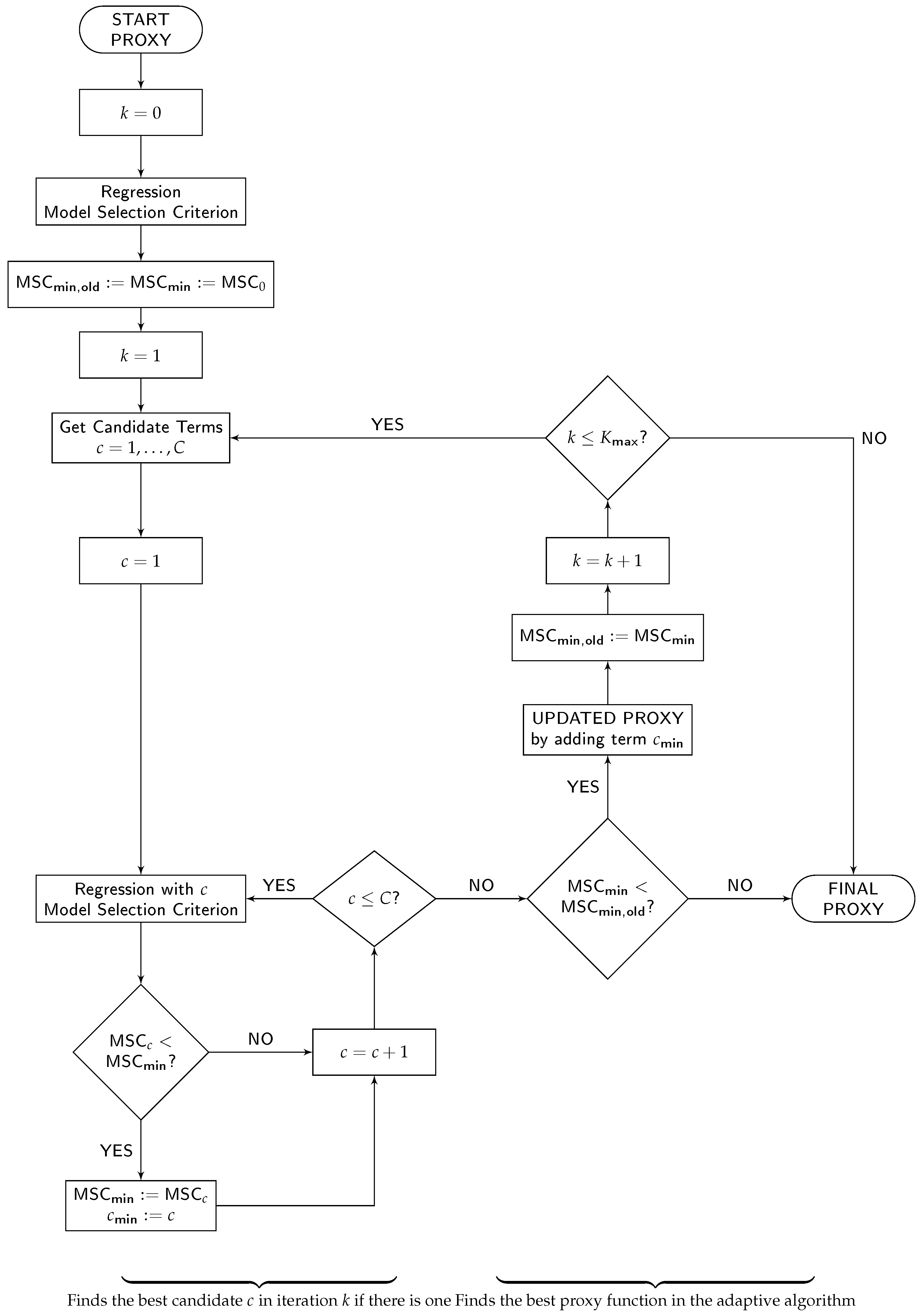
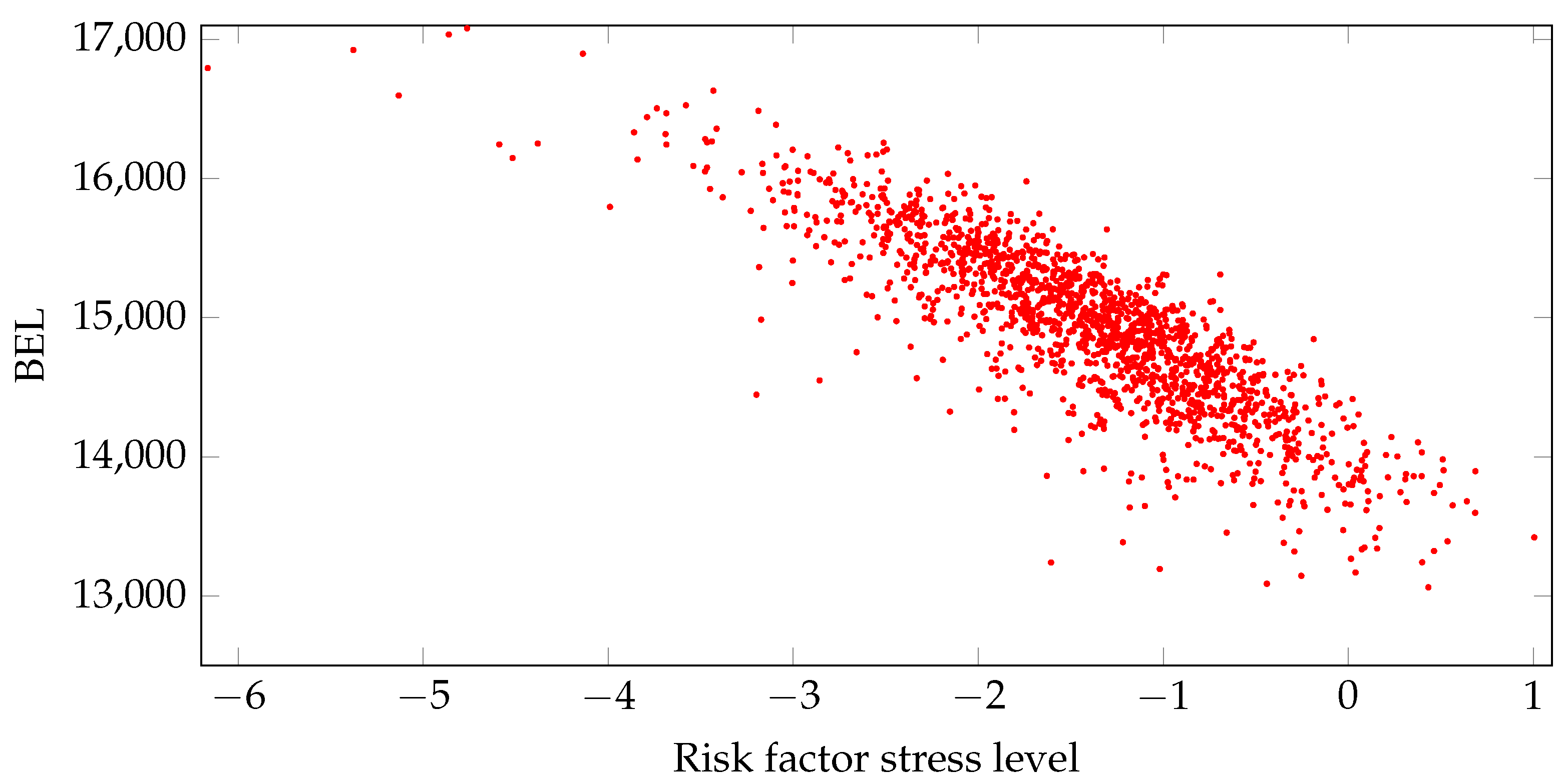
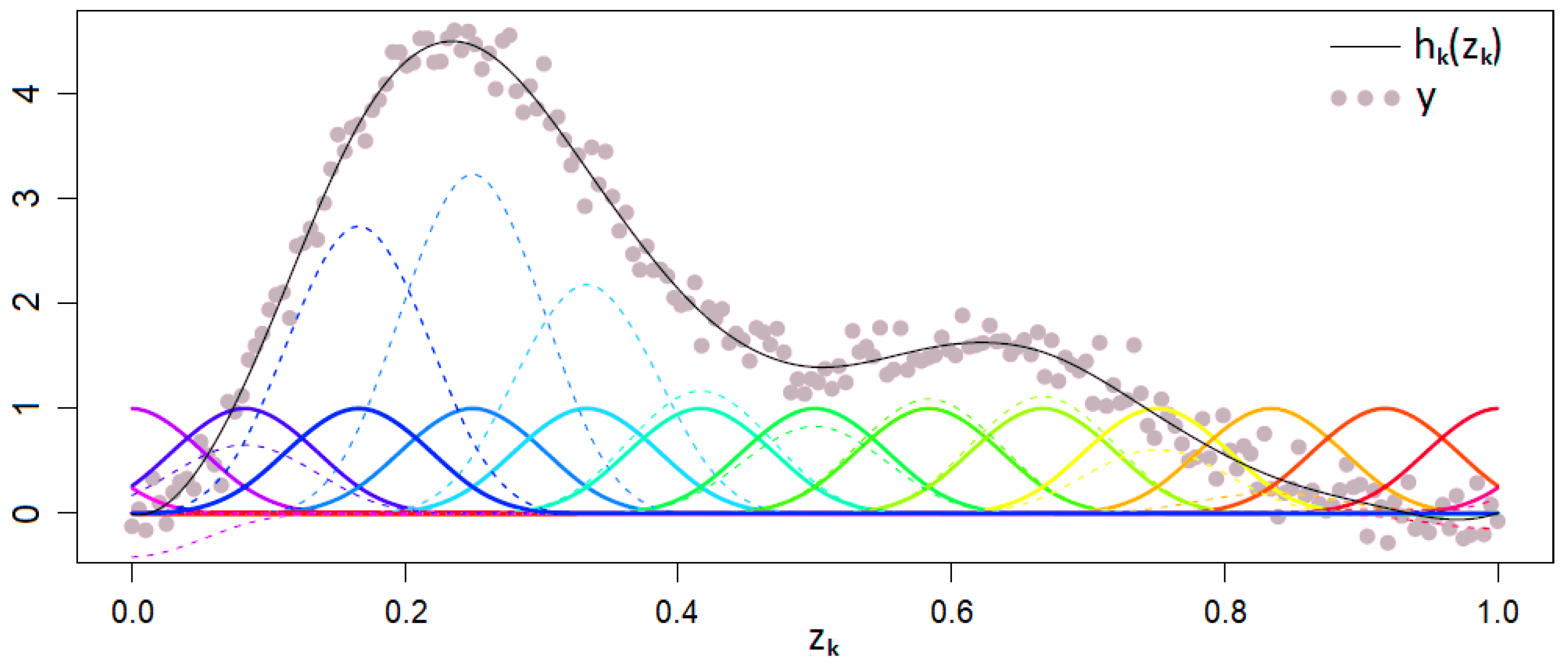
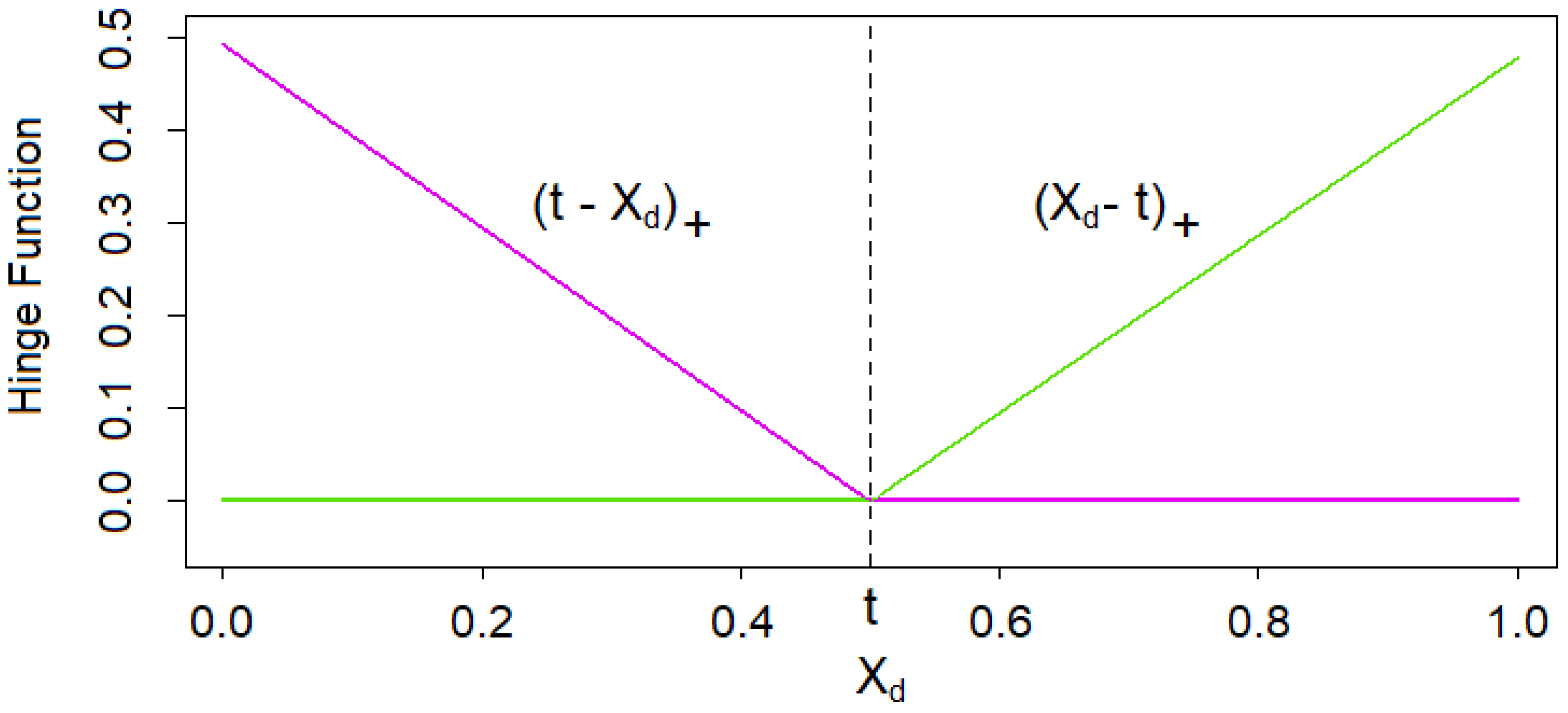
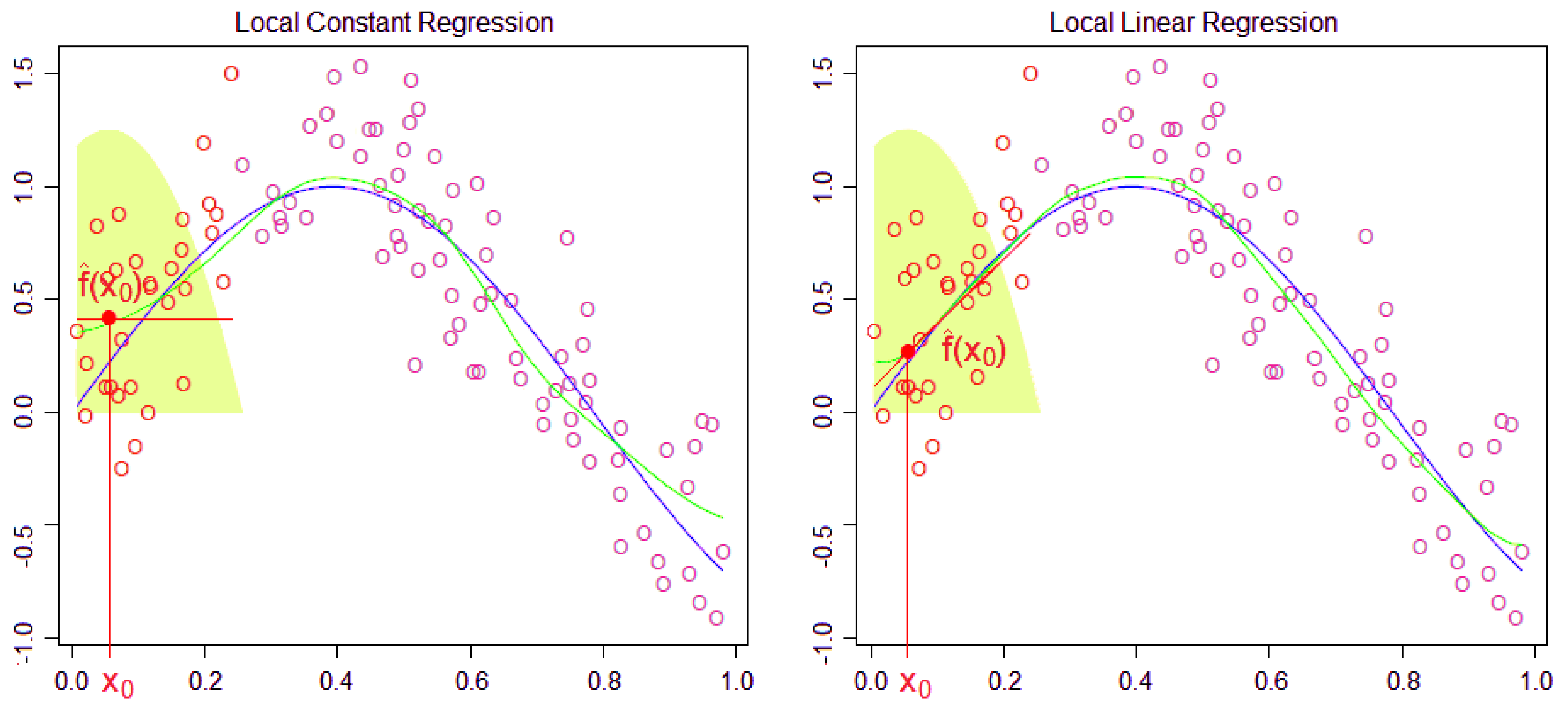
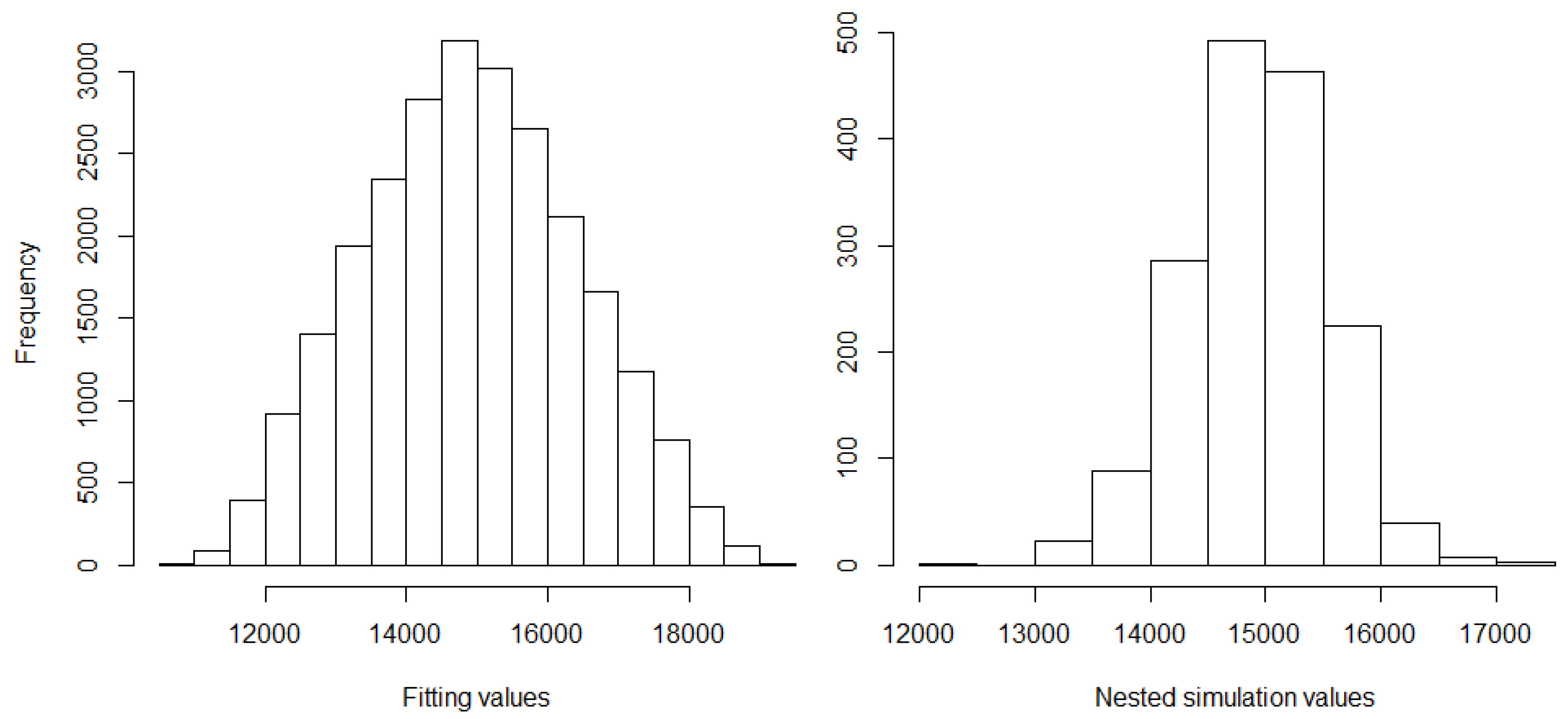
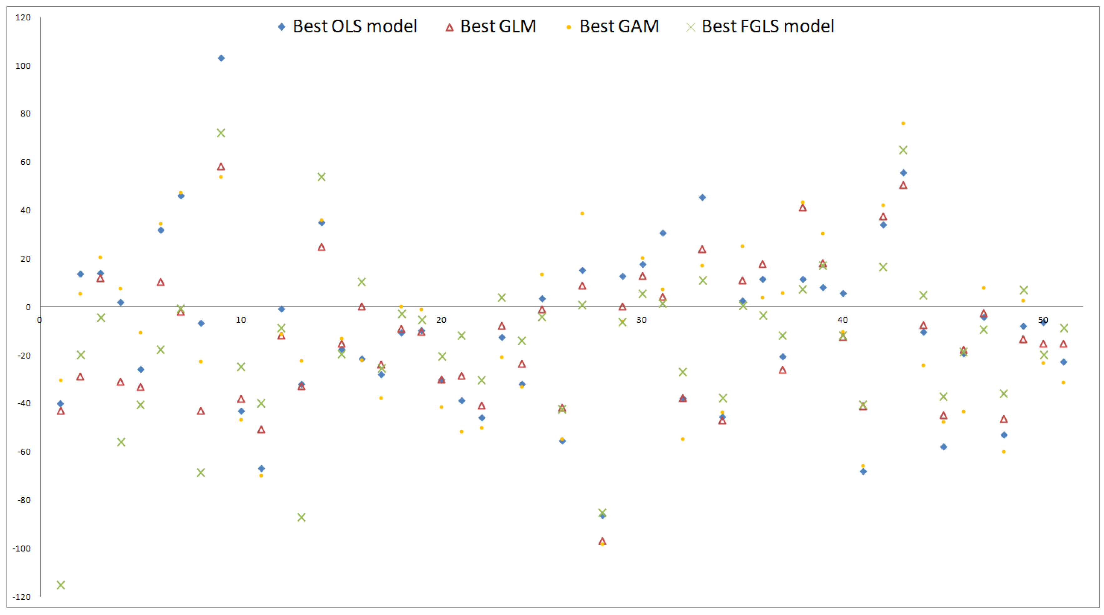
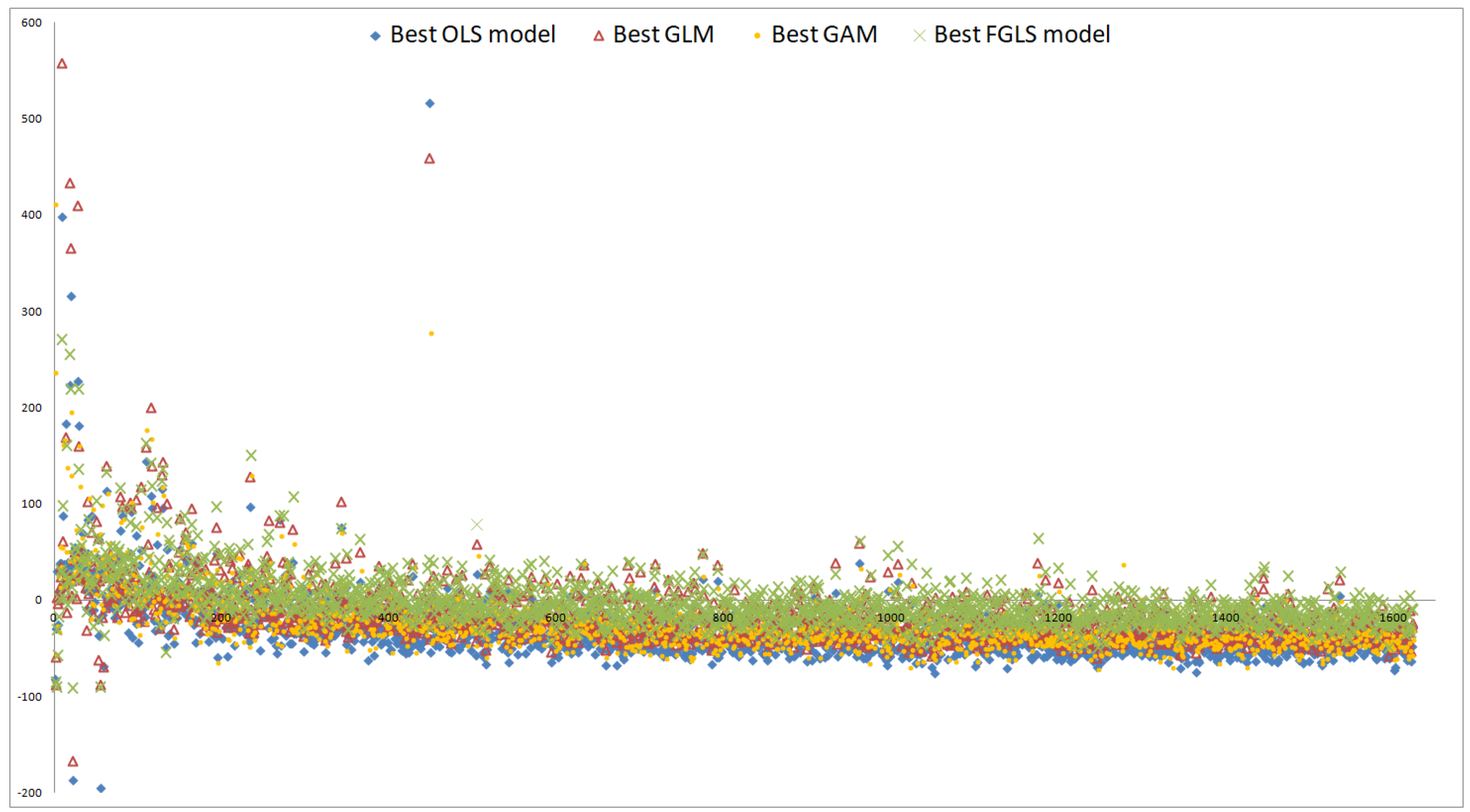
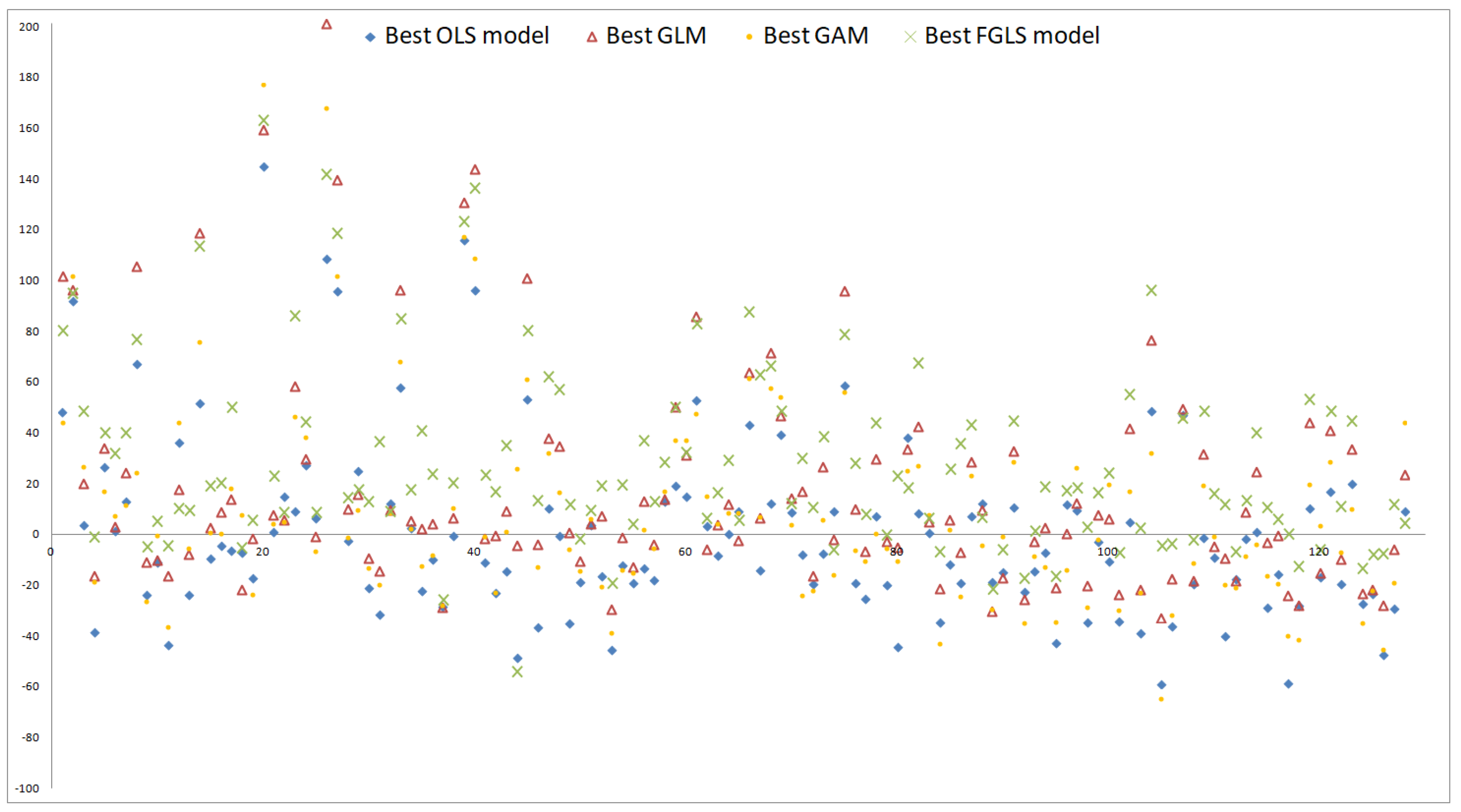
Table A1.
Ordinary least squares (OLS) proxy function of BEL derived under 150–443 in the adaptive algorithm with the final coefficients. Furthermore, Akaike information criterion (AIC) scores and out-of-sample mean absolute errors (MAEs) in % after each iteration.
Table A1.
Ordinary least squares (OLS) proxy function of BEL derived under 150–443 in the adaptive algorithm with the final coefficients. Furthermore, Akaike information criterion (AIC) scores and out-of-sample mean absolute errors (MAEs) in % after each iteration.
| k | AIC | v.mae | ns.mae | cr.mae | ||||||||||||||||
|---|---|---|---|---|---|---|---|---|---|---|---|---|---|---|---|---|---|---|---|---|
| 0 | 0 | 0 | 0 | 0 | 0 | 0 | 0 | 0 | 0 | 0 | 0 | 0 | 0 | 0 | 0 | 14,718.24 | 437,251 | 4.557 | 3.231 | 4.027 |
| 1 | 0 | 0 | 0 | 0 | 0 | 0 | 0 | 1 | 0 | 0 | 0 | 0 | 0 | 0 | 0 | 7850.17 | 386,722 | 2.474 | 0.845 | 0.913 |
| 2 | 1 | 0 | 0 | 0 | 0 | 0 | 0 | 0 | 0 | 0 | 0 | 0 | 0 | 0 | 0 | −269.33 | 375,144 | 2.065 | 2.139 | 1.831 |
| 3 | 0 | 0 | 0 | 0 | 0 | 1 | 0 | 0 | 0 | 0 | 0 | 0 | 0 | 0 | 0 | 145.21 | 366,567 | 1.656 | 0.444 | 0.496 |
| 4 | 0 | 0 | 0 | 0 | 0 | 0 | 0 | 0 | 0 | 0 | 0 | 0 | 0 | 0 | 1 | −5.36 | 358,894 | 1.647 | 1.006 | 0.556 |
| 5 | 0 | 0 | 0 | 0 | 0 | 0 | 1 | 0 | 0 | 0 | 0 | 0 | 0 | 0 | 0 | 434.04 | 355,732 | 1.635 | 0.853 | 0.469 |
| 6 | 1 | 0 | 0 | 0 | 0 | 0 | 0 | 1 | 0 | 0 | 0 | 0 | 0 | 0 | 0 | 1753.4 | 354,318 | 1.679 | 0.956 | 0.374 |
| 7 | 0 | 0 | 0 | 0 | 0 | 0 | 0 | 2 | 0 | 0 | 0 | 0 | 0 | 0 | 0 | 19,145.78 | 349,759 | 1.234 | 0.491 | 0.628 |
| 8 | 2 | 0 | 0 | 0 | 0 | 0 | 0 | 0 | 0 | 0 | 0 | 0 | 0 | 0 | 0 | 33.33 | 347,796 | 0.999 | 0.34 | 0.594 |
| 9 | 0 | 0 | 0 | 0 | 0 | 1 | 0 | 1 | 0 | 0 | 0 | 0 | 0 | 0 | 0 | 868.25 | 346,444 | 0.912 | 0.357 | 0.602 |
| 10 | 0 | 0 | 0 | 0 | 0 | 0 | 0 | 1 | 0 | 0 | 0 | 0 | 0 | 0 | 1 | 30.59 | 345,045 | 0.839 | 0.389 | 0.650 |
| 11 | 1 | 0 | 0 | 0 | 0 | 0 | 0 | 0 | 0 | 0 | 0 | 0 | 0 | 0 | 1 | 1.65 | 341,083 | 0.759 | 0.398 | 0.465 |
| 12 | 0 | 1 | 0 | 0 | 0 | 0 | 0 | 0 | 0 | 0 | 0 | 0 | 0 | 0 | 0 | 86.79 | 339,360 | 0.718 | 0.394 | 0.390 |
| 13 | 1 | 0 | 0 | 0 | 0 | 1 | 0 | 0 | 0 | 0 | 0 | 0 | 0 | 0 | 0 | 33.35 | 337,731 | 0.574 | 0.653 | 0.512 |
| 14 | 0 | 0 | 0 | 0 | 0 | 0 | 0 | 0 | 1 | 0 | 0 | 0 | 0 | 0 | 0 | 49.59 | 336,843 | 0.589 | 0.658 | 0.518 |
| 15 | 0 | 0 | 0 | 0 | 0 | 0 | 0 | 0 | 0 | 0 | 0 | 1 | 0 | 0 | 0 | 71.25 | 335,980 | 0.628 | 0.678 | 0.512 |
| 16 | 0 | 0 | 0 | 0 | 0 | 0 | 1 | 1 | 0 | 0 | 0 | 0 | 0 | 0 | 0 | 2667.92 | 335,351 | 0.609 | 0.671 | 0.503 |
| 17 | 1 | 0 | 0 | 0 | 0 | 0 | 1 | 0 | 0 | 0 | 0 | 0 | 0 | 0 | 0 | 96.43 | 334,876 | 0.579 | 0.701 | 0.545 |
| 18 | 1 | 0 | 0 | 0 | 0 | 0 | 0 | 1 | 0 | 0 | 0 | 0 | 0 | 0 | 1 | −6.31 | 334,413 | 0.593 | 0.72 | 0.531 |
| 19 | 0 | 0 | 0 | 0 | 0 | 0 | 0 | 2 | 0 | 0 | 0 | 0 | 0 | 0 | 1 | −47.09 | 333,904 | 0.562 | 0.621 | 0.474 |
| 20 | 0 | 0 | 0 | 0 | 0 | 0 | 0 | 0 | 0 | 0 | 0 | 0 | 0 | 1 | 0 | 48.93 | 333,447 | 0.565 | 0.597 | 0.454 |
| 21 | 1 | 0 | 0 | 0 | 0 | 0 | 0 | 2 | 0 | 0 | 0 | 0 | 0 | 0 | 0 | −3,412.68 | 333,116 | 0.553 | 0.543 | 0.407 |
| 22 | 0 | 0 | 0 | 0 | 0 | 0 | 0 | 0 | 0 | 0 | 0 | 0 | 0 | 0 | 2 | 0.02 | 332,806 | 0.562 | 0.478 | 0.358 |
| 23 | 2 | 0 | 0 | 0 | 0 | 0 | 0 | 0 | 0 | 0 | 0 | 0 | 0 | 0 | 1 | −0.12 | 332,547 | 0.55 | 0.45 | 0.381 |
| 24 | 0 | 0 | 0 | 0 | 0 | 0 | 0 | 0 | 0 | 0 | 0 | 0 | 1 | 0 | 0 | 43.77 | 332,294 | 0.545 | 0.468 | 0.378 |
| 25 | 0 | 0 | 1 | 0 | 0 | 0 | 0 | 0 | 0 | 0 | 0 | 0 | 0 | 0 | 0 | 118.94 | 332,042 | 0.53 | 0.464 | 0.362 |
| 26 | 0 | 0 | 1 | 0 | 0 | 0 | 0 | 1 | 0 | 0 | 0 | 0 | 0 | 0 | 0 | −1288.45 | 331,687 | 0.522 | 0.453 | 0.355 |
| 27 | 1 | 0 | 1 | 0 | 0 | 0 | 0 | 0 | 0 | 0 | 0 | 0 | 0 | 0 | 0 | −44.72 | 331,405 | 0.525 | 0.444 | 0.343 |
| 28 | 0 | 0 | 0 | 0 | 0 | 0 | 0 | 3 | 0 | 0 | 0 | 0 | 0 | 0 | 0 | −24,908.99 | 331,136 | 0.499 | 0.405 | 0.327 |
| 29 | 2 | 0 | 0 | 0 | 0 | 0 | 0 | 1 | 0 | 0 | 0 | 0 | 0 | 0 | 0 | −86.88 | 330,562 | 0.504 | 0.348 | 0.268 |
| 30 | 0 | 0 | 0 | 0 | 0 | 1 | 0 | 0 | 0 | 0 | 0 | 0 | 0 | 0 | 1 | 0.55 | 330,361 | 0.518 | 0.418 | 0.264 |
| 31 | 0 | 0 | 0 | 0 | 0 | 1 | 1 | 0 | 0 | 0 | 0 | 0 | 0 | 0 | 0 | 77.26 | 330,163 | 0.512 | 0.443 | 0.272 |
| 32 | 1 | 0 | 0 | 0 | 0 | 0 | 0 | 0 | 1 | 0 | 0 | 0 | 0 | 0 | 0 | 24.78 | 329,988 | 0.508 | 0.443 | 0.264 |
| 33 | 0 | 0 | 0 | 0 | 0 | 2 | 0 | 0 | 0 | 0 | 0 | 0 | 0 | 0 | 0 | 14.33 | 329,834 | 0.477 | 0.491 | 0.286 |
| 34 | 0 | 1 | 0 | 0 | 0 | 0 | 0 | 0 | 0 | 0 | 0 | 0 | 0 | 0 | 1 | −0.39 | 329,688 | 0.477 | 0.5 | 0.290 |
| 35 | 0 | 0 | 0 | 0 | 0 | 0 | 0 | 0 | 0 | 0 | 1 | 0 | 0 | 0 | 0 | 28.36 | 329,550 | 0.476 | 0.502 | 0.291 |
| 36 | 0 | 1 | 0 | 0 | 0 | 0 | 0 | 1 | 0 | 0 | 0 | 0 | 0 | 0 | 0 | −370.92 | 329,442 | 0.472 | 0.499 | 0.288 |
| 37 | 1 | 1 | 0 | 0 | 0 | 0 | 0 | 0 | 0 | 0 | 0 | 0 | 0 | 0 | 0 | −17.9 | 329,147 | 0.462 | 0.505 | 0.301 |
| 38 | 0 | 0 | 0 | 1 | 0 | 0 | 0 | 0 | 0 | 0 | 0 | 0 | 0 | 0 | 0 | 8574.53 | 329,043 | 0.472 | 0.518 | 0.3 |
| 39 | 0 | 0 | 0 | 0 | 0 | 1 | 0 | 1 | 0 | 0 | 0 | 0 | 0 | 0 | 1 | −2.17 | 328,935 | 0.474 | 0.51 | 0.295 |
| 40 | 0 | 0 | 0 | 0 | 0 | 0 | 0 | 1 | 1 | 0 | 0 | 0 | 0 | 0 | 0 | 223.91 | 328,832 | 0.475 | 0.509 | 0.291 |
| 41 | 0 | 0 | 0 | 0 | 0 | 1 | 0 | 2 | 0 | 0 | 0 | 0 | 0 | 0 | 0 | −1801.73 | 328,733 | 0.455 | 0.445 | 0.248 |
| 42 | 1 | 0 | 0 | 0 | 0 | 1 | 0 | 1 | 0 | 0 | 0 | 0 | 0 | 0 | 0 | −102.1 | 327,927 | 0.372 | 0.345 | 0.237 |
| 43 | 0 | 0 | 0 | 0 | 0 | 0 | 1 | 0 | 0 | 0 | 0 | 0 | 0 | 0 | 1 | 0.7 | 327,858 | 0.368 | 0.353 | 0.235 |
| 44 | 0 | 0 | 0 | 0 | 0 | 0 | 0 | 0 | 1 | 0 | 0 | 0 | 0 | 0 | 1 | 0.56 | 327,792 | 0.366 | 0.352 | 0.233 |
| 45 | 1 | 0 | 0 | 1 | 0 | 0 | 0 | 0 | 0 | 0 | 0 | 0 | 0 | 0 | 0 | −3034.32 | 327,729 | 0.365 | 0.356 | 0.228 |
| 46 | 0 | 0 | 0 | 1 | 0 | 0 | 0 | 1 | 0 | 0 | 0 | 0 | 0 | 0 | 0 | −13,127.81 | 327,659 | 0.368 | 0.364 | 0.227 |
| 47 | 1 | 0 | 0 | 0 | 0 | 0 | 0 | 0 | 0 | 0 | 0 | 1 | 0 | 0 | 0 | −17.54 | 327,603 | 0.368 | 0.366 | 0.226 |
| 48 | 0 | 0 | 0 | 0 | 0 | 0 | 0 | 1 | 0 | 0 | 0 | 1 | 0 | 0 | 0 | −187.07 | 327,537 | 0.374 | 0.367 | 0.226 |
| 49 | 0 | 0 | 0 | 0 | 0 | 1 | 1 | 1 | 0 | 0 | 0 | 0 | 0 | 0 | 0 | −300.54 | 327,483 | 0.369 | 0.367 | 0.230 |
| 50 | 1 | 0 | 0 | 0 | 0 | 1 | 0 | 0 | 0 | 0 | 0 | 0 | 0 | 0 | 1 | −0.09 | 327,432 | 0.368 | 0.391 | 0.221 |
| 51 | 0 | 0 | 0 | 0 | 0 | 2 | 0 | 1 | 0 | 0 | 0 | 0 | 0 | 0 | 0 | −60.84 | 327,382 | 0.359 | 0.39 | 0.228 |
| 52 | 0 | 0 | 1 | 0 | 0 | 1 | 0 | 0 | 0 | 0 | 0 | 0 | 0 | 0 | 0 | −20.91 | 327,331 | 0.352 | 0.39 | 0.225 |
| 53 | 1 | 0 | 0 | 0 | 0 | 0 | 0 | 0 | 0 | 0 | 0 | 0 | 0 | 0 | 2 | −0.0 | 327,287 | 0.346 | 0.377 | 0.206 |
| 54 | 0 | 0 | 0 | 0 | 0 | 0 | 0 | 1 | 0 | 0 | 0 | 0 | 0 | 0 | 2 | −0.09 | 327,149 | 0.339 | 0.357 | 0.185 |
| 55 | 2 | 0 | 0 | 0 | 0 | 1 | 0 | 0 | 0 | 0 | 0 | 0 | 0 | 0 | 0 | 1.44 | 327,105 | 0.315 | 0.321 | 0.173 |
| 56 | 0 | 0 | 1 | 0 | 0 | 0 | 0 | 0 | 0 | 0 | 0 | 0 | 0 | 0 | 1 | −0.5 | 327,064 | 0.315 | 0.322 | 0.173 |
| 57 | 1 | 0 | 0 | 0 | 0 | 0 | 0 | 0 | 0 | 0 | 0 | 0 | 0 | 1 | 0 | −6.06 | 327,025 | 0.322 | 0.317 | 0.175 |
| 58 | 0 | 0 | 0 | 0 | 0 | 0 | 1 | 2 | 0 | 0 | 0 | 0 | 0 | 0 | 0 | −6,600.49 | 326,986 | 0.317 | 0.31 | 0.172 |
| 59 | 1 | 0 | 0 | 0 | 0 | 0 | 1 | 1 | 0 | 0 | 0 | 0 | 0 | 0 | 0 | −407.57 | 326,823 | 0.308 | 0.302 | 0.183 |
| 60 | 0 | 0 | 1 | 0 | 0 | 0 | 0 | 2 | 0 | 0 | 0 | 0 | 0 | 0 | 0 | 3378.82 | 326,787 | 0.306 | 0.301 | 0.183 |
| 61 | 1 | 0 | 1 | 0 | 0 | 0 | 0 | 1 | 0 | 0 | 0 | 0 | 0 | 0 | 0 | 205.28 | 326,733 | 0.304 | 0.299 | 0.183 |
| 62 | 0 | 1 | 0 | 0 | 0 | 0 | 0 | 0 | 1 | 0 | 0 | 0 | 0 | 0 | 0 | −18.73 | 326,700 | 0.306 | 0.299 | 0.182 |
| 63 | 0 | 0 | 1 | 0 | 0 | 1 | 0 | 1 | 0 | 0 | 0 | 0 | 0 | 0 | 0 | 175.39 | 326,668 | 0.304 | 0.296 | 0.182 |
| 64 | 0 | 0 | 0 | 0 | 0 | 0 | 0 | 0 | 0 | 0 | 0 | 1 | 0 | 0 | 1 | −0.2 | 326,638 | 0.304 | 0.298 | 0.181 |
| 65 | 0 | 1 | 0 | 0 | 0 | 0 | 0 | 1 | 0 | 0 | 0 | 0 | 0 | 0 | 1 | 2.45 | 326,610 | 0.301 | 0.296 | 0.183 |
| 66 | 1 | 1 | 0 | 0 | 0 | 0 | 0 | 0 | 0 | 0 | 0 | 0 | 0 | 0 | 1 | 0.11 | 326,572 | 0.297 | 0.299 | 0.180 |
| 67 | 2 | 0 | 0 | 0 | 0 | 1 | 0 | 1 | 0 | 0 | 0 | 0 | 0 | 0 | 0 | −13.02 | 326,545 | 0.292 | 0.286 | 0.169 |
| 68 | 1 | 1 | 0 | 0 | 0 | 0 | 0 | 1 | 0 | 0 | 0 | 0 | 0 | 0 | 0 | 93.69 | 326,519 | 0.292 | 0.287 | 0.172 |
| 69 | 0 | 1 | 0 | 0 | 0 | 0 | 0 | 2 | 0 | 0 | 0 | 0 | 0 | 0 | 0 | 891.58 | 326,478 | 0.294 | 0.282 | 0.173 |
| 70 | 0 | 0 | 0 | 0 | 0 | 0 | 1 | 1 | 0 | 0 | 0 | 0 | 0 | 0 | 1 | −6.21 | 326,453 | 0.291 | 0.281 | 0.175 |
| 71 | 0 | 0 | 0 | 0 | 0 | 0 | 0 | 1 | 0 | 0 | 1 | 0 | 0 | 0 | 0 | −112.56 | 326,428 | 0.289 | 0.281 | 0.176 |
| 72 | 1 | 0 | 0 | 0 | 0 | 0 | 0 | 0 | 0 | 0 | 1 | 0 | 0 | 0 | 0 | −5.27 | 326,398 | 0.284 | 0.282 | 0.173 |
| 73 | 1 | 0 | 0 | 0 | 0 | 0 | 0 | 3 | 0 | 0 | 0 | 0 | 0 | 0 | 0 | 1129.77 | 326,374 | 0.276 | 0.264 | 0.162 |
| 74 | 1 | 0 | 0 | 0 | 0 | 0 | 1 | 0 | 0 | 0 | 0 | 0 | 0 | 0 | 1 | −0.29 | 326,352 | 0.272 | 0.266 | 0.158 |
| 75 | 1 | 0 | 0 | 0 | 0 | 0 | 0 | 1 | 1 | 0 | 0 | 0 | 0 | 0 | 0 | −56.54 | 326,331 | 0.269 | 0.266 | 0.157 |
| 76 | 2 | 0 | 0 | 0 | 0 | 0 | 0 | 0 | 1 | 0 | 0 | 0 | 0 | 0 | 0 | −3.02 | 326,313 | 0.271 | 0.266 | 0.155 |
| 77 | 1 | 0 | 0 | 0 | 0 | 1 | 1 | 0 | 0 | 0 | 0 | 0 | 0 | 0 | 0 | −10.59 | 326,295 | 0.264 | 0.27 | 0.151 |
| 78 | 0 | 1 | 0 | 0 | 0 | 1 | 0 | 0 | 0 | 0 | 0 | 0 | 0 | 0 | 0 | −6.99 | 326,278 | 0.264 | 0.275 | 0.153 |
| 79 | 1 | 0 | 0 | 0 | 0 | 2 | 0 | 0 | 0 | 0 | 0 | 0 | 0 | 0 | 0 | −2.25 | 326,261 | 0.252 | 0.285 | 0.154 |
| 80 | 0 | 0 | 0 | 0 | 0 | 0 | 0 | 0 | 2 | 0 | 0 | 0 | 0 | 0 | 0 | −14.77 | 326,245 | 0.263 | 0.309 | 0.157 |
| 81 | 2 | 1 | 0 | 0 | 0 | 0 | 0 | 0 | 0 | 0 | 0 | 0 | 0 | 0 | 0 | 1.95 | 326,229 | 0.267 | 0.306 | 0.155 |
| 82 | 0 | 1 | 0 | 1 | 0 | 0 | 0 | 0 | 0 | 0 | 0 | 0 | 0 | 0 | 0 | 2248.54 | 326,214 | 0.266 | 0.307 | 0.156 |
| 83 | 0 | 0 | 0 | 0 | 0 | 0 | 0 | 3 | 0 | 0 | 0 | 0 | 0 | 0 | 1 | −111.77 | 326,201 | 0.263 | 0.302 | 0.158 |
| 84 | 1 | 0 | 0 | 0 | 0 | 0 | 0 | 0 | 1 | 0 | 0 | 0 | 0 | 0 | 1 | −0.11 | 326,187 | 0.262 | 0.302 | 0.157 |
| 85 | 0 | 0 | 0 | 0 | 0 | 0 | 0 | 0 | 0 | 0 | 0 | 0 | 1 | 0 | 1 | −0.18 | 326,174 | 0.263 | 0.305 | 0.156 |
| 86 | 0 | 1 | 0 | 0 | 0 | 1 | 0 | 1 | 0 | 0 | 0 | 0 | 0 | 0 | 0 | 45.58 | 326,161 | 0.265 | 0.303 | 0.157 |
| 87 | 0 | 0 | 0 | 1 | 0 | 0 | 0 | 2 | 0 | 0 | 0 | 0 | 0 | 0 | 0 | −83,291.89 | 326,149 | 0.267 | 0.308 | 0.156 |
| 88 | 0 | 0 | 1 | 0 | 0 | 0 | 1 | 0 | 0 | 0 | 0 | 0 | 0 | 0 | 0 | −56.2 | 326,137 | 0.267 | 0.308 | 0.156 |
| 89 | 1 | 0 | 0 | 0 | 0 | 0 | 0 | 0 | 0 | 0 | 0 | 0 | 1 | 0 | 0 | −5.32 | 326,126 | 0.267 | 0.31 | 0.156 |
| 90 | 0 | 0 | 0 | 0 | 0 | 2 | 1 | 0 | 0 | 0 | 0 | 0 | 0 | 0 | 0 | −10.87 | 326,116 | 0.267 | 0.313 | 0.158 |
| 91 | 0 | 0 | 0 | 1 | 0 | 0 | 0 | 0 | 0 | 0 | 0 | 0 | 0 | 0 | 1 | −32.75 | 326,106 | 0.265 | 0.317 | 0.158 |
| 92 | 0 | 0 | 0 | 0 | 0 | 0 | 0 | 2 | 0 | 0 | 0 | 0 | 0 | 0 | 2 | −0.09 | 326,097 | 0.265 | 0.308 | 0.151 |
| 93 | 0 | 1 | 0 | 0 | 0 | 0 | 0 | 0 | 0 | 0 | 0 | 0 | 0 | 1 | 0 | 10.87 | 326,089 | 0.265 | 0.308 | 0.151 |
| 94 | 1 | 0 | 0 | 0 | 0 | 1 | 1 | 1 | 0 | 0 | 0 | 0 | 0 | 0 | 0 | −48.93 | 326,081 | 0.264 | 0.306 | 0.148 |
| 95 | 0 | 0 | 0 | 0 | 0 | 0 | 2 | 0 | 0 | 0 | 0 | 0 | 0 | 0 | 0 | 69.57 | 326,073 | 0.256 | 0.288 | 0.141 |
| 96 | 0 | 0 | 0 | 1 | 0 | 0 | 0 | 3 | 0 | 0 | 0 | 0 | 0 | 0 | 0 | −542,688.19 | 326,066 | 0.256 | 0.289 | 0.141 |
| 97 | 0 | 0 | 0 | 0 | 0 | 0 | 0 | 0 | 0 | 0 | 0 | 0 | 0 | 2 | 0 | 10.44 | 326,058 | 0.248 | 0.275 | 0.136 |
| 98 | 0 | 0 | 0 | 0 | 0 | 0 | 0 | 1 | 1 | 0 | 0 | 0 | 0 | 0 | 1 | −1.08 | 326,051 | 0.248 | 0.276 | 0.136 |
| 99 | 0 | 0 | 1 | 0 | 0 | 0 | 1 | 1 | 0 | 0 | 0 | 0 | 0 | 0 | 0 | 419.05 | 326,045 | 0.249 | 0.275 | 0.136 |
| 100 | 0 | 1 | 1 | 0 | 0 | 0 | 0 | 0 | 0 | 0 | 0 | 0 | 0 | 0 | 0 | 12.8 | 326,038 | 0.25 | 0.276 | 0.136 |
| 101 | 0 | 0 | 0 | 0 | 0 | 1 | 0 | 0 | 0 | 0 | 1 | 0 | 0 | 0 | 0 | −3.94 | 326,033 | 0.25 | 0.276 | 0.136 |
| 102 | 1 | 0 | 0 | 0 | 0 | 0 | 0 | 2 | 0 | 0 | 0 | 0 | 0 | 0 | 1 | −10.12 | 326,027 | 0.248 | 0.281 | 0.138 |
| 103 | 2 | 0 | 0 | 0 | 0 | 0 | 0 | 1 | 0 | 0 | 0 | 0 | 0 | 0 | 1 | −0.36 | 326,017 | 0.244 | 0.283 | 0.135 |
| 104 | 0 | 0 | 1 | 0 | 0 | 0 | 0 | 1 | 0 | 0 | 0 | 0 | 0 | 0 | 1 | 1.74 | 326,012 | 0.244 | 0.282 | 0.136 |
| 105 | 0 | 0 | 0 | 0 | 0 | 0 | 0 | 0 | 0 | 0 | 0 | 0 | 0 | 0 | 3 | −0.0 | 326,006 | 0.242 | 0.268 | 0.132 |
| 106 | 2 | 0 | 0 | 0 | 0 | 0 | 1 | 0 | 0 | 0 | 0 | 0 | 0 | 0 | 0 | −7.09 | 326,001 | 0.238 | 0.265 | 0.131 |
| 107 | 2 | 0 | 0 | 0 | 0 | 0 | 1 | 1 | 0 | 0 | 0 | 0 | 0 | 0 | 0 | −109.46 | 325,982 | 0.238 | 0.263 | 0.129 |
| 108 | 0 | 0 | 0 | 0 | 0 | 0 | 0 | 0 | 0 | 0 | 1 | 0 | 0 | 0 | 1 | −0.1 | 325,977 | 0.237 | 0.263 | 0.128 |
| 109 | 0 | 1 | 0 | 0 | 0 | 0 | 0 | 0 | 0 | 0 | 0 | 1 | 0 | 0 | 0 | 5.76 | 325,972 | 0.235 | 0.263 | 0.129 |
| 110 | 1 | 0 | 0 | 0 | 0 | 0 | 0 | 1 | 0 | 0 | 1 | 0 | 0 | 0 | 0 | 54.51 | 325,968 | 0.237 | 0.264 | 0.129 |
| 111 | 1 | 0 | 0 | 0 | 0 | 0 | 1 | 2 | 0 | 0 | 0 | 0 | 0 | 0 | 0 | −1386.73 | 325,963 | 0.235 | 0.264 | 0.129 |
| 112 | 0 | 0 | 0 | 0 | 0 | 0 | 0 | 0 | 1 | 0 | 0 | 0 | 0 | 0 | 2 | −0.0 | 325,959 | 0.237 | 0.265 | 0.13 |
| 113 | 0 | 1 | 0 | 0 | 0 | 0 | 0 | 0 | 1 | 0 | 0 | 0 | 0 | 0 | 1 | 0.11 | 325,955 | 0.235 | 0.265 | 0.13 |
| 114 | 0 | 1 | 0 | 0 | 0 | 1 | 0 | 0 | 0 | 0 | 0 | 0 | 0 | 0 | 1 | 0.05 | 325,951 | 0.234 | 0.266 | 0.13 |
| 115 | 1 | 0 | 1 | 0 | 0 | 1 | 0 | 0 | 0 | 0 | 0 | 0 | 0 | 0 | 0 | 4.3 | 325,948 | 0.236 | 0.265 | 0.127 |
| 116 | 1 | 0 | 0 | 0 | 0 | 2 | 0 | 1 | 0 | 0 | 0 | 0 | 0 | 0 | 0 | −19.81 | 325,944 | 0.237 | 0.262 | 0.126 |
| 117 | 2 | 0 | 0 | 0 | 0 | 2 | 0 | 0 | 0 | 0 | 0 | 0 | 0 | 0 | 0 | −0.87 | 325,938 | 0.241 | 0.267 | 0.124 |
| 118 | 0 | 1 | 0 | 0 | 0 | 1 | 0 | 1 | 0 | 0 | 0 | 0 | 0 | 0 | 1 | −0.36 | 325,935 | 0.241 | 0.267 | 0.124 |
| 119 | 0 | 1 | 1 | 0 | 0 | 0 | 0 | 1 | 0 | 0 | 0 | 0 | 0 | 0 | 0 | −80.29 | 325,931 | 0.241 | 0.267 | 0.125 |
| 120 | 0 | 0 | 0 | 0 | 0 | 0 | 0 | 0 | 1 | 0 | 0 | 0 | 1 | 0 | 0 | −6.95 | 325,928 | 0.241 | 0.267 | 0.124 |
| 121 | 0 | 0 | 0 | 0 | 0 | 1 | 0 | 0 | 0 | 0 | 0 | 0 | 0 | 0 | 2 | −0.0 | 325,925 | 0.243 | 0.259 | 0.121 |
| 122 | 0 | 0 | 0 | 0 | 0 | 0 | 0 | 2 | 0 | 0 | 1 | 0 | 0 | 0 | 0 | 436.56 | 325,923 | 0.241 | 0.259 | 0.121 |
| 123 | 0 | 0 | 0 | 0 | 0 | 2 | 0 | 0 | 0 | 0 | 0 | 0 | 0 | 0 | 1 | −0.03 | 325,920 | 0.243 | 0.263 | 0.121 |
| 124 | 0 | 0 | 0 | 0 | 0 | 1 | 0 | 0 | 1 | 0 | 0 | 0 | 0 | 0 | 0 | 2.99 | 325,918 | 0.242 | 0.263 | 0.12 |
| 125 | 1 | 0 | 0 | 0 | 0 | 1 | 0 | 1 | 0 | 0 | 0 | 0 | 0 | 0 | 1 | −0.59 | 325,916 | 0.241 | 0.261 | 0.119 |
| 126 | 2 | 0 | 0 | 0 | 0 | 1 | 0 | 0 | 0 | 0 | 0 | 0 | 0 | 0 | 1 | −0.02 | 325,908 | 0.247 | 0.265 | 0.124 |
| 127 | 0 | 0 | 0 | 0 | 0 | 1 | 0 | 2 | 0 | 0 | 0 | 0 | 0 | 0 | 1 | −4.66 | 325,902 | 0.249 | 0.279 | 0.123 |
| 128 | 0 | 0 | 0 | 0 | 0 | 0 | 1 | 3 | 0 | 0 | 0 | 0 | 0 | 0 | 0 | −8179.68 | 325,900 | 0.249 | 0.28 | 0.124 |
| 129 | 0 | 0 | 0 | 0 | 0 | 1 | 0 | 3 | 0 | 0 | 0 | 0 | 0 | 0 | 0 | 691.4 | 325,898 | 0.249 | 0.28 | 0.123 |
| 130 | 1 | 0 | 0 | 0 | 0 | 0 | 0 | 0 | 0 | 0 | 0 | 0 | 1 | 0 | 1 | 0.04 | 325,896 | 0.25 | 0.281 | 0.122 |
| 131 | 0 | 0 | 0 | 0 | 0 | 0 | 0 | 0 | 0 | 1 | 0 | 0 | 0 | 0 | 0 | 7.04 | 325,894 | 0.246 | 0.264 | 0.12 |
| 132 | 0 | 0 | 1 | 0 | 0 | 0 | 0 | 0 | 0 | 1 | 0 | 0 | 0 | 0 | 0 | −27.72 | 325,892 | 0.247 | 0.264 | 0.119 |
| 133 | 2 | 0 | 0 | 0 | 0 | 0 | 0 | 0 | 0 | 0 | 1 | 0 | 0 | 0 | 0 | 1.26 | 325,891 | 0.247 | 0.264 | 0.119 |
| 134 | 0 | 0 | 0 | 0 | 0 | 1 | 0 | 0 | 0 | 0 | 0 | 1 | 0 | 0 | 0 | −2.67 | 325,889 | 0.249 | 0.265 | 0.118 |
| 135 | 1 | 0 | 0 | 0 | 0 | 1 | 0 | 0 | 0 | 0 | 0 | 1 | 0 | 0 | 0 | 1.53 | 325,887 | 0.25 | 0.266 | 0.119 |
| 136 | 0 | 0 | 0 | 0 | 0 | 0 | 0 | 0 | 0 | 0 | 0 | 0 | 0 | 1 | 1 | −0.07 | 325,885 | 0.25 | 0.265 | 0.12 |
| 137 | 1 | 0 | 0 | 0 | 0 | 0 | 0 | 1 | 0 | 0 | 0 | 1 | 0 | 0 | 0 | 40.44 | 325,884 | 0.251 | 0.265 | 0.119 |
| 138 | 0 | 0 | 0 | 0 | 0 | 0 | 0 | 2 | 0 | 0 | 0 | 1 | 0 | 0 | 0 | 434.5 | 325,878 | 0.249 | 0.264 | 0.119 |
| 139 | 0 | 0 | 0 | 0 | 0 | 0 | 0 | 0 | 1 | 0 | 0 | 1 | 0 | 0 | 0 | −5.99 | 325,877 | 0.248 | 0.264 | 0.119 |
| 140 | 0 | 0 | 0 | 0 | 0 | 0 | 0 | 0 | 2 | 0 | 0 | 1 | 0 | 0 | 0 | 14.64 | 325,873 | 0.246 | 0.263 | 0.12 |
| 141 | 0 | 0 | 0 | 0 | 0 | 2 | 0 | 2 | 0 | 0 | 0 | 0 | 0 | 0 | 0 | −119.42 | 325,871 | 0.247 | 0.27 | 0.121 |
| 142 | 0 | 0 | 0 | 0 | 0 | 0 | 0 | 1 | 0 | 0 | 0 | 0 | 0 | 0 | 3 | 0.0 | 325,870 | 0.248 | 0.271 | 0.121 |
| 143 | 1 | 0 | 0 | 0 | 0 | 0 | 0 | 0 | 0 | 0 | 0 | 1 | 0 | 0 | 1 | 0.07 | 325,868 | 0.248 | 0.271 | 0.121 |
| 144 | 0 | 0 | 0 | 0 | 0 | 0 | 0 | 1 | 0 | 0 | 0 | 1 | 0 | 0 | 1 | 1.06 | 325,861 | 0.246 | 0.271 | 0.121 |
| 145 | 1 | 0 | 0 | 0 | 0 | 0 | 1 | 1 | 0 | 0 | 0 | 0 | 0 | 0 | 1 | −0.74 | 325,859 | 0.247 | 0.271 | 0.121 |
| 146 | 0 | 0 | 0 | 0 | 0 | 0 | 0 | 0 | 1 | 0 | 0 | 0 | 0 | 1 | 0 | −5.61 | 325,858 | 0.246 | 0.271 | 0.121 |
| 147 | 0 | 1 | 0 | 0 | 0 | 0 | 0 | 0 | 0 | 0 | 0 | 0 | 0 | 1 | 1 | −0.08 | 325,857 | 0.247 | 0.27 | 0.121 |
| 148 | 0 | 0 | 0 | 0 | 0 | 0 | 1 | 0 | 0 | 0 | 0 | 0 | 1 | 0 | 0 | −37.16 | 325,855 | 0.247 | 0.271 | 0.122 |
| 149 | 0 | 0 | 0 | 0 | 0 | 0 | 1 | 0 | 0 | 0 | 0 | 0 | 1 | 0 | 1 | 0.41 | 325,851 | 0.247 | 0.271 | 0.122 |
| 150 | 0 | 1 | 0 | 1 | 0 | 0 | 0 | 1 | 0 | 0 | 0 | 0 | 0 | 0 | 0 | −7290.99 | 325,850 | 0.247 | 0.271 | 0.122 |
Table A2.
OLS proxy function of available capital (AC) derived under 150–443 in the adaptive algorithm with the final coefficients. Furthermore, AIC scores and out-of-sample MAEs in % after each iteration.
Table A2.
OLS proxy function of available capital (AC) derived under 150–443 in the adaptive algorithm with the final coefficients. Furthermore, AIC scores and out-of-sample MAEs in % after each iteration.
| k | AIC | v.mae | ns.mae | cr.mae | ||||||||||||||||
|---|---|---|---|---|---|---|---|---|---|---|---|---|---|---|---|---|---|---|---|---|
| 0 | 0 | 0 | 0 | 0 | 0 | 0 | 0 | 0 | 0 | 0 | 0 | 0 | 0 | 0 | 0 | 745.35 | 391,375 | 60.62 | 97.518 | 257.762 |
| 1 | 0 | 0 | 0 | 0 | 0 | 0 | 0 | 1 | 0 | 0 | 0 | 0 | 0 | 0 | 0 | 5766.61 | 382,610 | 50.402 | 99.306 | 256.789 |
| 2 | 1 | 0 | 0 | 0 | 0 | 0 | 0 | 0 | 0 | 0 | 0 | 0 | 0 | 0 | 0 | 272.75 | 367,667 | 35.285 | 38.124 | 99.902 |
| 3 | 0 | 0 | 0 | 0 | 0 | 0 | 0 | 0 | 0 | 0 | 0 | 0 | 0 | 0 | 1 | 5.46 | 359,997 | 30.739 | 18.21 | 72.719 |
| 4 | 0 | 0 | 0 | 0 | 0 | 1 | 0 | 0 | 0 | 0 | 0 | 0 | 0 | 0 | 0 | 128.41 | 356,705 | 30.119 | 25.088 | 29.357 |
| 5 | 1 | 0 | 0 | 0 | 0 | 0 | 0 | 1 | 0 | 0 | 0 | 0 | 0 | 0 | 0 | −1750.72 | 355,354 | 30.867 | 28.173 | 21.870 |
| 6 | 0 | 0 | 0 | 0 | 0 | 0 | 0 | 2 | 0 | 0 | 0 | 0 | 0 | 0 | 0 | −19,127.27 | 351,002 | 22.942 | 14.948 | 44.668 |
| 7 | 2 | 0 | 0 | 0 | 0 | 0 | 0 | 0 | 0 | 0 | 0 | 0 | 0 | 0 | 0 | −33.25 | 349,147 | 19.03 | 12.142 | 42.535 |
| 8 | 0 | 0 | 0 | 0 | 0 | 0 | 1 | 0 | 0 | 0 | 0 | 0 | 0 | 0 | 0 | 307.32 | 347,777 | 18.221 | 10.928 | 35.420 |
| 9 | 0 | 0 | 0 | 0 | 0 | 1 | 0 | 1 | 0 | 0 | 0 | 0 | 0 | 0 | 0 | −868.05 | 346,423 | 16.662 | 11.527 | 35.941 |
| 10 | 0 | 1 | 0 | 0 | 0 | 0 | 0 | 0 | 0 | 0 | 0 | 0 | 0 | 0 | 0 | −87.54 | 345,025 | 15.987 | 10.264 | 31.461 |
| 11 | 0 | 0 | 0 | 0 | 0 | 0 | 0 | 1 | 0 | 0 | 0 | 0 | 0 | 0 | 1 | −30.51 | 343,570 | 14.858 | 11.187 | 34.502 |
| 12 | 1 | 0 | 0 | 0 | 0 | 0 | 0 | 0 | 0 | 0 | 0 | 0 | 0 | 0 | 1 | −1.66 | 339,282 | 13.092 | 12.669 | 23.174 |
| 13 | 1 | 0 | 0 | 0 | 0 | 1 | 0 | 0 | 0 | 0 | 0 | 0 | 0 | 0 | 0 | −33.33 | 337,648 | 10.427 | 20.976 | 30.402 |
| 14 | 0 | 0 | 0 | 0 | 0 | 0 | 0 | 0 | 0 | 0 | 0 | 1 | 0 | 0 | 0 | −70.63 | 336,840 | 11.087 | 21.598 | 29.972 |
| 15 | 0 | 0 | 0 | 0 | 0 | 0 | 0 | 0 | 1 | 0 | 0 | 0 | 0 | 0 | 0 | −41.37 | 336,120 | 11.436 | 21.764 | 30.408 |
| 16 | 0 | 0 | 0 | 0 | 0 | 0 | 1 | 1 | 0 | 0 | 0 | 0 | 0 | 0 | 0 | −2666.44 | 335,495 | 11.088 | 21.543 | 29.890 |
| 17 | 1 | 0 | 0 | 0 | 0 | 0 | 1 | 0 | 0 | 0 | 0 | 0 | 0 | 0 | 0 | −96.48 | 335,022 | 10.545 | 22.479 | 32.334 |
| 18 | 1 | 0 | 0 | 0 | 0 | 0 | 0 | 1 | 0 | 0 | 0 | 0 | 0 | 0 | 1 | 6.3 | 334,563 | 10.804 | 23.095 | 31.519 |
| 19 | 0 | 0 | 0 | 0 | 0 | 0 | 0 | 2 | 0 | 0 | 0 | 0 | 0 | 0 | 1 | 47.02 | 334,058 | 10.232 | 19.913 | 28.128 |
| 20 | 0 | 0 | 0 | 0 | 0 | 0 | 0 | 0 | 0 | 0 | 0 | 0 | 0 | 1 | 0 | −48.77 | 333,610 | 10.292 | 19.163 | 26.995 |
| 21 | 1 | 0 | 0 | 0 | 0 | 0 | 0 | 2 | 0 | 0 | 0 | 0 | 0 | 0 | 0 | 3412.54 | 333,281 | 10.083 | 17.438 | 24.190 |
| 22 | 0 | 0 | 0 | 0 | 0 | 0 | 0 | 0 | 0 | 0 | 0 | 0 | 0 | 0 | 2 | −0.02 | 332,970 | 10.246 | 15.328 | 21.326 |
| 23 | 2 | 0 | 0 | 0 | 0 | 0 | 0 | 0 | 0 | 0 | 0 | 0 | 0 | 0 | 1 | 0.12 | 332,714 | 10.02 | 14.436 | 22.671 |
| 24 | 0 | 0 | 1 | 0 | 0 | 0 | 0 | 0 | 0 | 0 | 0 | 0 | 0 | 0 | 0 | −120.68 | 332,457 | 9.834 | 14.283 | 21.608 |
| 25 | 0 | 0 | 1 | 0 | 0 | 0 | 0 | 1 | 0 | 0 | 0 | 0 | 0 | 0 | 0 | 1287.63 | 332,108 | 9.725 | 13.969 | 21.273 |
| 26 | 1 | 0 | 1 | 0 | 0 | 0 | 0 | 0 | 0 | 0 | 0 | 0 | 0 | 0 | 0 | 44.71 | 331,832 | 9.755 | 13.661 | 20.501 |
| 27 | 0 | 0 | 0 | 0 | 0 | 0 | 0 | 3 | 0 | 0 | 0 | 0 | 0 | 0 | 0 | 24,899.66 | 331,569 | 9.275 | 12.462 | 19.873 |
| 28 | 2 | 0 | 0 | 0 | 0 | 0 | 0 | 1 | 0 | 0 | 0 | 0 | 0 | 0 | 0 | 87.04 | 331,004 | 9.292 | 10.757 | 17.022 |
| 29 | 0 | 0 | 0 | 0 | 0 | 0 | 0 | 0 | 0 | 0 | 0 | 0 | 1 | 0 | 0 | −43.38 | 330,742 | 9.171 | 11.183 | 16.023 |
| 30 | 0 | 0 | 0 | 0 | 0 | 1 | 0 | 0 | 0 | 0 | 0 | 0 | 0 | 0 | 1 | −0.55 | 330,543 | 9.444 | 13.409 | 15.766 |
| 31 | 0 | 0 | 0 | 0 | 0 | 1 | 1 | 0 | 0 | 0 | 0 | 0 | 0 | 0 | 0 | −77.35 | 330,345 | 9.324 | 14.207 | 16.192 |
| 32 | 1 | 0 | 0 | 0 | 0 | 0 | 0 | 0 | 1 | 0 | 0 | 0 | 0 | 0 | 0 | −25.2 | 330,161 | 9.246 | 14.203 | 15.692 |
| 33 | 0 | 0 | 0 | 0 | 0 | 2 | 0 | 0 | 0 | 0 | 0 | 0 | 0 | 0 | 0 | −14.37 | 330,007 | 8.672 | 15.764 | 16.964 |
| 34 | 0 | 1 | 0 | 0 | 0 | 0 | 0 | 0 | 0 | 0 | 0 | 0 | 0 | 0 | 1 | 0.39 | 329,859 | 8.682 | 16.031 | 17.223 |
| 35 | 0 | 0 | 0 | 0 | 0 | 0 | 0 | 0 | 0 | 0 | 1 | 0 | 0 | 0 | 0 | −27.8 | 329,728 | 8.665 | 16.11 | 17.264 |
| 36 | 0 | 0 | 0 | 1 | 0 | 0 | 0 | 0 | 0 | 0 | 0 | 0 | 0 | 0 | 0 | −8757.49 | 329,619 | 8.871 | 16.53 | 17.005 |
| 37 | 0 | 0 | 0 | 0 | 0 | 1 | 0 | 1 | 0 | 0 | 0 | 0 | 0 | 0 | 1 | 2.17 | 329,513 | 8.937 | 16.276 | 16.790 |
| 38 | 0 | 1 | 0 | 0 | 0 | 0 | 0 | 1 | 0 | 0 | 0 | 0 | 0 | 0 | 0 | 369.16 | 329,408 | 8.842 | 16.169 | 16.738 |
| 39 | 1 | 1 | 0 | 0 | 0 | 0 | 0 | 0 | 0 | 0 | 0 | 0 | 0 | 0 | 0 | 17.97 | 329,109 | 8.637 | 16.387 | 17.527 |
| 40 | 0 | 0 | 0 | 0 | 0 | 0 | 0 | 1 | 1 | 0 | 0 | 0 | 0 | 0 | 0 | −222.55 | 329,008 | 8.656 | 16.359 | 17.271 |
| 41 | 0 | 0 | 0 | 0 | 0 | 1 | 0 | 2 | 0 | 0 | 0 | 0 | 0 | 0 | 0 | 1791.7 | 328,910 | 8.297 | 14.282 | 14.748 |
| 42 | 1 | 0 | 0 | 0 | 0 | 1 | 0 | 1 | 0 | 0 | 0 | 0 | 0 | 0 | 0 | 101.23 | 328,111 | 6.783 | 11.112 | 14.144 |
| 43 | 0 | 0 | 0 | 0 | 0 | 0 | 1 | 0 | 0 | 0 | 0 | 0 | 0 | 0 | 1 | −0.7 | 328,041 | 6.713 | 11.355 | 14.013 |
| 44 | 0 | 0 | 0 | 0 | 0 | 0 | 0 | 0 | 1 | 0 | 0 | 0 | 0 | 0 | 1 | −0.57 | 327,972 | 6.683 | 11.325 | 13.867 |
| 45 | 1 | 0 | 0 | 1 | 0 | 0 | 0 | 0 | 0 | 0 | 0 | 0 | 0 | 0 | 0 | 3083.05 | 327,905 | 6.654 | 11.456 | 13.595 |
| 46 | 0 | 0 | 0 | 1 | 0 | 0 | 0 | 1 | 0 | 0 | 0 | 0 | 0 | 0 | 0 | 12,863.79 | 327,837 | 6.7 | 11.721 | 13.5 |
| 47 | 1 | 0 | 0 | 0 | 0 | 0 | 0 | 0 | 0 | 0 | 0 | 1 | 0 | 0 | 0 | 17.78 | 327,780 | 6.71 | 11.777 | 13.450 |
| 48 | 0 | 0 | 0 | 0 | 0 | 0 | 0 | 1 | 0 | 0 | 0 | 1 | 0 | 0 | 0 | 190.46 | 327,711 | 6.824 | 11.818 | 13.468 |
| 49 | 0 | 0 | 0 | 0 | 0 | 1 | 1 | 1 | 0 | 0 | 0 | 0 | 0 | 0 | 0 | 300.76 | 327,657 | 6.724 | 11.793 | 13.716 |
| 50 | 1 | 0 | 0 | 0 | 0 | 1 | 0 | 0 | 0 | 0 | 0 | 0 | 0 | 0 | 1 | 0.09 | 327,607 | 6.718 | 12.565 | 13.182 |
| 51 | 0 | 0 | 0 | 0 | 0 | 2 | 0 | 1 | 0 | 0 | 0 | 0 | 0 | 0 | 0 | 60.83 | 327,557 | 6.543 | 12.533 | 13.558 |
| 52 | 0 | 0 | 1 | 0 | 0 | 1 | 0 | 0 | 0 | 0 | 0 | 0 | 0 | 0 | 0 | 20.91 | 327,507 | 6.415 | 12.53 | 13.394 |
| 53 | 1 | 0 | 0 | 0 | 0 | 0 | 0 | 0 | 0 | 0 | 0 | 0 | 0 | 0 | 2 | 0.0 | 327,463 | 6.314 | 12.118 | 12.252 |
| 54 | 0 | 0 | 0 | 0 | 0 | 0 | 0 | 1 | 0 | 0 | 0 | 0 | 0 | 0 | 2 | 0.08 | 327,327 | 6.176 | 11.486 | 11.049 |
| 55 | 2 | 0 | 0 | 0 | 0 | 1 | 0 | 0 | 0 | 0 | 0 | 0 | 0 | 0 | 0 | −1.46 | 327,284 | 5.751 | 10.339 | 10.295 |
| 56 | 0 | 0 | 1 | 0 | 0 | 0 | 0 | 0 | 0 | 0 | 0 | 0 | 0 | 0 | 1 | 0.5 | 327,242 | 5.746 | 10.367 | 10.287 |
| 57 | 1 | 0 | 0 | 0 | 0 | 0 | 0 | 0 | 0 | 0 | 0 | 0 | 0 | 1 | 0 | 6.08 | 327,203 | 5.871 | 10.211 | 10.450 |
| 58 | 0 | 0 | 0 | 0 | 0 | 0 | 1 | 2 | 0 | 0 | 0 | 0 | 0 | 0 | 0 | 6593.98 | 327,165 | 5.78 | 9.973 | 10.274 |
| 59 | 1 | 0 | 0 | 0 | 0 | 0 | 1 | 1 | 0 | 0 | 0 | 0 | 0 | 0 | 0 | 406.73 | 327,003 | 5.618 | 9.722 | 10.897 |
| 60 | 0 | 0 | 1 | 0 | 0 | 0 | 0 | 2 | 0 | 0 | 0 | 0 | 0 | 0 | 0 | −3,364.02 | 326,968 | 5.581 | 9.671 | 10.904 |
| 61 | 1 | 0 | 1 | 0 | 0 | 0 | 0 | 1 | 0 | 0 | 0 | 0 | 0 | 0 | 0 | −204.12 | 326,914 | 5.542 | 9.626 | 10.921 |
| 62 | 0 | 1 | 0 | 0 | 0 | 0 | 0 | 0 | 1 | 0 | 0 | 0 | 0 | 0 | 0 | 18.9 | 326,881 | 5.588 | 9.611 | 10.837 |
| 63 | 0 | 0 | 1 | 0 | 0 | 1 | 0 | 1 | 0 | 0 | 0 | 0 | 0 | 0 | 0 | −175.17 | 326,849 | 5.546 | 9.514 | 10.817 |
| 64 | 0 | 0 | 0 | 0 | 0 | 0 | 0 | 0 | 0 | 0 | 0 | 1 | 0 | 0 | 1 | 0.21 | 326,818 | 5.54 | 9.597 | 10.799 |
| 65 | 0 | 1 | 0 | 0 | 0 | 0 | 0 | 1 | 0 | 0 | 0 | 0 | 0 | 0 | 1 | −2.44 | 326,791 | 5.494 | 9.532 | 10.896 |
| 66 | 1 | 1 | 0 | 0 | 0 | 0 | 0 | 0 | 0 | 0 | 0 | 0 | 0 | 0 | 1 | −0.11 | 326,753 | 5.413 | 9.616 | 10.708 |
| 67 | 2 | 0 | 0 | 0 | 0 | 1 | 0 | 1 | 0 | 0 | 0 | 0 | 0 | 0 | 0 | 12.99 | 326,726 | 5.317 | 9.215 | 10.046 |
| 68 | 1 | 1 | 0 | 0 | 0 | 0 | 0 | 1 | 0 | 0 | 0 | 0 | 0 | 0 | 0 | −93.57 | 326,700 | 5.329 | 9.255 | 10.231 |
| 69 | 0 | 1 | 0 | 0 | 0 | 0 | 0 | 2 | 0 | 0 | 0 | 0 | 0 | 0 | 0 | −890.62 | 326,660 | 5.355 | 9.09 | 10.326 |
| 70 | 0 | 0 | 0 | 0 | 0 | 0 | 0 | 1 | 0 | 0 | 1 | 0 | 0 | 0 | 0 | 113.04 | 326,635 | 5.313 | 9.095 | 10.357 |
| 71 | 1 | 0 | 0 | 0 | 0 | 0 | 0 | 0 | 0 | 0 | 1 | 0 | 0 | 0 | 0 | 5.23 | 326,605 | 5.231 | 9.101 | 10.164 |
| 72 | 0 | 0 | 0 | 0 | 0 | 0 | 1 | 1 | 0 | 0 | 0 | 0 | 0 | 0 | 1 | 6.2 | 326,581 | 5.186 | 9.068 | 10.265 |
| 73 | 1 | 0 | 0 | 0 | 0 | 0 | 0 | 3 | 0 | 0 | 0 | 0 | 0 | 0 | 0 | −1,133.83 | 326,556 | 5.034 | 8.488 | 9.647 |
| 74 | 1 | 0 | 0 | 0 | 0 | 0 | 1 | 0 | 0 | 0 | 0 | 0 | 0 | 0 | 1 | 0.29 | 326,534 | 4.95 | 8.58 | 9.374 |
| 75 | 1 | 0 | 0 | 0 | 0 | 0 | 0 | 1 | 1 | 0 | 0 | 0 | 0 | 0 | 0 | 56.56 | 326,513 | 4.908 | 8.559 | 9.323 |
| 76 | 2 | 0 | 0 | 0 | 0 | 0 | 0 | 0 | 1 | 0 | 0 | 0 | 0 | 0 | 0 | 3.02 | 326,495 | 4.936 | 8.573 | 9.223 |
| 77 | 1 | 0 | 0 | 0 | 0 | 1 | 1 | 0 | 0 | 0 | 0 | 0 | 0 | 0 | 0 | 10.61 | 326,477 | 4.824 | 8.705 | 8.996 |
| 78 | 0 | 1 | 0 | 0 | 0 | 1 | 0 | 0 | 0 | 0 | 0 | 0 | 0 | 0 | 0 | 6.97 | 326,461 | 4.821 | 8.849 | 9.071 |
| 79 | 1 | 0 | 0 | 0 | 0 | 2 | 0 | 0 | 0 | 0 | 0 | 0 | 0 | 0 | 0 | 2.25 | 326,444 | 4.602 | 9.17 | 9.162 |
| 80 | 2 | 1 | 0 | 0 | 0 | 0 | 0 | 0 | 0 | 0 | 0 | 0 | 0 | 0 | 0 | −1.94 | 326,429 | 4.688 | 9.069 | 8.997 |
| 81 | 0 | 1 | 0 | 1 | 0 | 0 | 0 | 0 | 0 | 0 | 0 | 0 | 0 | 0 | 0 | −2,257.4 | 326,414 | 4.676 | 9.099 | 9.070 |
| 82 | 0 | 0 | 0 | 0 | 0 | 0 | 0 | 0 | 2 | 0 | 0 | 0 | 0 | 0 | 0 | 14.06 | 326,399 | 4.853 | 9.831 | 9.278 |
| 83 | 1 | 0 | 0 | 0 | 0 | 0 | 0 | 0 | 1 | 0 | 0 | 0 | 0 | 0 | 1 | 0.11 | 326,385 | 4.844 | 9.851 | 9.203 |
| 84 | 0 | 0 | 0 | 0 | 0 | 0 | 0 | 0 | 0 | 0 | 0 | 0 | 1 | 0 | 1 | 0.18 | 326,372 | 4.861 | 9.935 | 9.174 |
| 85 | 0 | 0 | 0 | 0 | 0 | 0 | 0 | 3 | 0 | 0 | 0 | 0 | 0 | 0 | 1 | 111.58 | 326,358 | 4.796 | 9.769 | 9.270 |
| 86 | 0 | 1 | 0 | 0 | 0 | 1 | 0 | 1 | 0 | 0 | 0 | 0 | 0 | 0 | 0 | −45.11 | 326,346 | 4.826 | 9.724 | 9.330 |
| 87 | 0 | 0 | 0 | 1 | 0 | 0 | 0 | 2 | 0 | 0 | 0 | 0 | 0 | 0 | 0 | 82,935.66 | 326,334 | 4.871 | 9.865 | 9.284 |
| 88 | 0 | 0 | 1 | 0 | 0 | 0 | 1 | 0 | 0 | 0 | 0 | 0 | 0 | 0 | 0 | 56.0 | 326,322 | 4.867 | 9.862 | 9.267 |
| 89 | 1 | 0 | 0 | 0 | 0 | 0 | 0 | 0 | 0 | 0 | 0 | 0 | 1 | 0 | 0 | 5.35 | 326,311 | 4.857 | 9.938 | 9.258 |
| 90 | 0 | 0 | 0 | 0 | 0 | 2 | 1 | 0 | 0 | 0 | 0 | 0 | 0 | 0 | 0 | 10.88 | 326,301 | 4.87 | 10.043 | 9.414 |
| 91 | 0 | 0 | 0 | 1 | 0 | 0 | 0 | 0 | 0 | 0 | 0 | 0 | 0 | 0 | 1 | 32.81 | 326,291 | 4.833 | 10.156 | 9.394 |
| 92 | 1 | 0 | 0 | 0 | 0 | 1 | 1 | 1 | 0 | 0 | 0 | 0 | 0 | 0 | 0 | 48.96 | 326,283 | 4.812 | 10.085 | 9.185 |
| 93 | 0 | 1 | 0 | 0 | 0 | 0 | 0 | 0 | 0 | 0 | 0 | 0 | 0 | 1 | 0 | −10.9 | 326,274 | 4.801 | 10.083 | 9.210 |
| 94 | 0 | 0 | 0 | 0 | 0 | 0 | 0 | 2 | 0 | 0 | 0 | 0 | 0 | 0 | 2 | 0.09 | 326,266 | 4.803 | 9.818 | 8.787 |
| 95 | 0 | 0 | 0 | 0 | 0 | 0 | 2 | 0 | 0 | 0 | 0 | 0 | 0 | 0 | 0 | −69.45 | 326,258 | 4.659 | 9.25 | 8.413 |
| 96 | 0 | 0 | 0 | 1 | 0 | 0 | 0 | 3 | 0 | 0 | 0 | 0 | 0 | 0 | 0 | 543,840.26 | 326,251 | 4.663 | 9.269 | 8.393 |
| 97 | 0 | 0 | 0 | 0 | 0 | 0 | 0 | 0 | 0 | 0 | 0 | 0 | 0 | 2 | 0 | −10.31 | 326,244 | 4.51 | 8.841 | 8.101 |
| 98 | 0 | 0 | 0 | 0 | 0 | 0 | 0 | 1 | 1 | 0 | 0 | 0 | 0 | 0 | 1 | 1.07 | 326,237 | 4.523 | 8.847 | 8.091 |
| 99 | 0 | 0 | 1 | 0 | 0 | 0 | 1 | 1 | 0 | 0 | 0 | 0 | 0 | 0 | 0 | −417.88 | 326,231 | 4.531 | 8.84 | 8.101 |
| 100 | 0 | 1 | 1 | 0 | 0 | 0 | 0 | 0 | 0 | 0 | 0 | 0 | 0 | 0 | 0 | −12.92 | 326,224 | 4.546 | 8.847 | 8.081 |
| 101 | 0 | 0 | 0 | 0 | 0 | 1 | 0 | 0 | 0 | 0 | 1 | 0 | 0 | 0 | 0 | 3.94 | 326,219 | 4.558 | 8.866 | 8.072 |
| 102 | 1 | 0 | 0 | 0 | 0 | 0 | 0 | 2 | 0 | 0 | 0 | 0 | 0 | 0 | 1 | 10.1 | 326,213 | 4.513 | 9.012 | 8.203 |
| 103 | 2 | 0 | 0 | 0 | 0 | 0 | 0 | 1 | 0 | 0 | 0 | 0 | 0 | 0 | 1 | 0.36 | 326,204 | 4.453 | 9.084 | 8.035 |
| 104 | 0 | 0 | 1 | 0 | 0 | 0 | 0 | 1 | 0 | 0 | 0 | 0 | 0 | 0 | 1 | −1.74 | 326,198 | 4.445 | 9.063 | 8.070 |
| 105 | 2 | 0 | 0 | 0 | 0 | 0 | 1 | 0 | 0 | 0 | 0 | 0 | 0 | 0 | 0 | 7.09 | 326,193 | 4.383 | 8.967 | 8.008 |
| 106 | 2 | 0 | 0 | 0 | 0 | 0 | 1 | 1 | 0 | 0 | 0 | 0 | 0 | 0 | 0 | 109.5 | 326,174 | 4.371 | 8.899 | 7.889 |
| 107 | 0 | 0 | 0 | 0 | 0 | 0 | 0 | 0 | 0 | 0 | 0 | 0 | 0 | 0 | 3 | 0.0 | 326,169 | 4.332 | 8.454 | 7.669 |
| 108 | 0 | 1 | 0 | 0 | 0 | 0 | 0 | 0 | 0 | 0 | 0 | 1 | 0 | 0 | 0 | −5.85 | 326,164 | 4.29 | 8.456 | 7.689 |
| 109 | 0 | 0 | 0 | 0 | 0 | 0 | 0 | 0 | 0 | 0 | 1 | 0 | 0 | 0 | 1 | 0.1 | 326,159 | 4.282 | 8.457 | 7.657 |
| 110 | 1 | 0 | 0 | 0 | 0 | 0 | 0 | 1 | 0 | 0 | 1 | 0 | 0 | 0 | 0 | −54.88 | 326,154 | 4.313 | 8.463 | 7.689 |
| 111 | 1 | 0 | 0 | 0 | 0 | 0 | 1 | 2 | 0 | 0 | 0 | 0 | 0 | 0 | 0 | 1380.74 | 326,150 | 4.291 | 8.489 | 7.7 |
| 112 | 0 | 0 | 0 | 0 | 0 | 0 | 0 | 0 | 1 | 0 | 0 | 0 | 0 | 0 | 2 | 0.0 | 326,146 | 4.315 | 8.498 | 7.751 |
| 113 | 0 | 1 | 0 | 0 | 0 | 0 | 0 | 0 | 1 | 0 | 0 | 0 | 0 | 0 | 1 | −0.11 | 326,142 | 4.287 | 8.501 | 7.736 |
| 114 | 1 | 0 | 1 | 0 | 0 | 1 | 0 | 0 | 0 | 0 | 0 | 0 | 0 | 0 | 0 | −4.3 | 326,138 | 4.32 | 8.461 | 7.558 |
| 115 | 0 | 1 | 0 | 0 | 0 | 1 | 0 | 0 | 0 | 0 | 0 | 0 | 0 | 0 | 1 | −0.05 | 326,135 | 4.299 | 8.514 | 7.566 |
| 116 | 1 | 0 | 0 | 0 | 0 | 2 | 0 | 1 | 0 | 0 | 0 | 0 | 0 | 0 | 0 | 20.09 | 326,131 | 4.32 | 8.417 | 7.498 |
| 117 | 2 | 0 | 0 | 0 | 0 | 2 | 0 | 0 | 0 | 0 | 0 | 0 | 0 | 0 | 0 | 0.87 | 326,125 | 4.393 | 8.561 | 7.371 |
| 118 | 0 | 1 | 0 | 0 | 0 | 1 | 0 | 1 | 0 | 0 | 0 | 0 | 0 | 0 | 1 | 0.36 | 326,122 | 4.389 | 8.564 | 7.409 |
| 119 | 0 | 1 | 1 | 0 | 0 | 0 | 0 | 1 | 0 | 0 | 0 | 0 | 0 | 0 | 0 | 79.51 | 326,118 | 4.394 | 8.56 | 7.411 |
| 120 | 0 | 0 | 0 | 0 | 0 | 1 | 0 | 0 | 0 | 0 | 0 | 0 | 0 | 0 | 2 | 0.0 | 326,115 | 4.43 | 8.304 | 7.187 |
| 121 | 0 | 0 | 0 | 0 | 0 | 0 | 0 | 0 | 1 | 0 | 0 | 0 | 1 | 0 | 0 | 6.91 | 326,113 | 4.42 | 8.305 | 7.176 |
| 122 | 0 | 0 | 0 | 0 | 0 | 0 | 0 | 2 | 0 | 0 | 1 | 0 | 0 | 0 | 0 | −435.81 | 326,110 | 4.39 | 8.301 | 7.212 |
| 123 | 0 | 0 | 0 | 0 | 0 | 2 | 0 | 0 | 0 | 0 | 0 | 0 | 0 | 0 | 1 | 0.03 | 326,107 | 4.419 | 8.45 | 7.206 |
| 124 | 0 | 0 | 0 | 0 | 0 | 1 | 0 | 0 | 1 | 0 | 0 | 0 | 0 | 0 | 0 | −2.99 | 326,105 | 4.407 | 8.434 | 7.163 |
| 125 | 1 | 0 | 0 | 0 | 0 | 1 | 0 | 1 | 0 | 0 | 0 | 0 | 0 | 0 | 1 | 0.59 | 326,103 | 4.394 | 8.366 | 7.095 |
| 126 | 2 | 0 | 0 | 0 | 0 | 1 | 0 | 0 | 0 | 0 | 0 | 0 | 0 | 0 | 1 | 0.02 | 326,096 | 4.502 | 8.499 | 7.382 |
| 127 | 0 | 0 | 0 | 0 | 0 | 1 | 0 | 2 | 0 | 0 | 0 | 0 | 0 | 0 | 1 | 4.66 | 326,089 | 4.543 | 8.962 | 7.340 |
| 128 | 0 | 0 | 0 | 0 | 0 | 1 | 0 | 3 | 0 | 0 | 0 | 0 | 0 | 0 | 0 | −692.59 | 326,088 | 4.537 | 8.961 | 7.248 |
| 129 | 0 | 0 | 0 | 0 | 0 | 0 | 1 | 3 | 0 | 0 | 0 | 0 | 0 | 0 | 0 | 8097.7 | 326,086 | 4.539 | 8.995 | 7.316 |
| 130 | 1 | 0 | 0 | 0 | 0 | 0 | 0 | 0 | 0 | 0 | 0 | 0 | 1 | 0 | 1 | −0.04 | 326,084 | 4.555 | 9.024 | 7.285 |
| 131 | 0 | 0 | 0 | 0 | 0 | 1 | 0 | 0 | 0 | 0 | 0 | 1 | 0 | 0 | 0 | 2.73 | 326,082 | 4.59 | 9.065 | 7.246 |
| 132 | 1 | 0 | 0 | 0 | 0 | 1 | 0 | 0 | 0 | 0 | 0 | 1 | 0 | 0 | 0 | −1.53 | 326,080 | 4.612 | 9.097 | 7.280 |
| 133 | 2 | 0 | 0 | 0 | 0 | 0 | 0 | 0 | 0 | 0 | 1 | 0 | 0 | 0 | 0 | −1.28 | 326,078 | 4.616 | 9.086 | 7.251 |
| 134 | 0 | 0 | 0 | 0 | 0 | 0 | 0 | 0 | 0 | 0 | 0 | 0 | 0 | 1 | 1 | 0.07 | 326,077 | 4.607 | 9.055 | 7.287 |
| 135 | 0 | 0 | 0 | 0 | 0 | 0 | 0 | 0 | 0 | 1 | 0 | 0 | 0 | 0 | 0 | −6.96 | 326,075 | 4.533 | 8.527 | 7.230 |
| 136 | 0 | 0 | 1 | 0 | 0 | 0 | 0 | 0 | 0 | 1 | 0 | 0 | 0 | 0 | 0 | 27.74 | 326,073 | 4.556 | 8.52 | 7.115 |
| 137 | 0 | 0 | 0 | 0 | 0 | 2 | 0 | 2 | 0 | 0 | 0 | 0 | 0 | 0 | 0 | 122.08 | 326,071 | 4.571 | 8.746 | 7.171 |
| 138 | 0 | 0 | 0 | 0 | 0 | 0 | 0 | 0 | 1 | 0 | 0 | 1 | 0 | 0 | 0 | 6.0 | 326,070 | 4.556 | 8.745 | 7.190 |
| 139 | 0 | 0 | 0 | 0 | 0 | 0 | 0 | 0 | 2 | 0 | 0 | 1 | 0 | 0 | 0 | −14.5 | 326,066 | 4.533 | 8.699 | 7.199 |
| 140 | 1 | 0 | 0 | 0 | 0 | 0 | 0 | 0 | 0 | 0 | 0 | 1 | 0 | 0 | 1 | −0.07 | 326,064 | 4.532 | 8.722 | 7.227 |
| 141 | 0 | 0 | 0 | 0 | 0 | 0 | 0 | 1 | 0 | 0 | 0 | 1 | 0 | 0 | 1 | −1.05 | 326,057 | 4.507 | 8.733 | 7.250 |
| 142 | 1 | 0 | 0 | 0 | 0 | 0 | 1 | 1 | 0 | 0 | 0 | 0 | 0 | 0 | 1 | 0.74 | 326,056 | 4.515 | 8.719 | 7.238 |
| 143 | 0 | 0 | 0 | 0 | 0 | 0 | 0 | 0 | 1 | 0 | 0 | 0 | 0 | 1 | 0 | 5.71 | 326,054 | 4.503 | 8.706 | 7.263 |
| 144 | 1 | 0 | 0 | 0 | 0 | 0 | 0 | 1 | 0 | 0 | 0 | 1 | 0 | 0 | 0 | −39.87 | 326,053 | 4.499 | 8.715 | 7.244 |
| 145 | 0 | 0 | 0 | 0 | 0 | 0 | 0 | 2 | 0 | 0 | 0 | 1 | 0 | 0 | 0 | −431.71 | 326,047 | 4.47 | 8.669 | 7.215 |
| 146 | 0 | 0 | 0 | 0 | 0 | 0 | 0 | 1 | 0 | 0 | 0 | 0 | 0 | 0 | 3 | −0.0 | 326,046 | 4.488 | 8.698 | 7.207 |
| 147 | 0 | 1 | 0 | 0 | 0 | 0 | 0 | 0 | 0 | 0 | 0 | 0 | 0 | 1 | 1 | 0.08 | 326,045 | 4.494 | 8.694 | 7.223 |
| 148 | 0 | 0 | 0 | 0 | 0 | 0 | 1 | 0 | 0 | 0 | 0 | 0 | 1 | 0 | 0 | 37.33 | 326,043 | 4.496 | 8.703 | 7.236 |
| 149 | 0 | 0 | 0 | 0 | 0 | 0 | 1 | 0 | 0 | 0 | 0 | 0 | 1 | 0 | 1 | −0.42 | 326,039 | 4.508 | 8.706 | 7.253 |
| 150 | 0 | 1 | 0 | 1 | 0 | 0 | 0 | 1 | 0 | 0 | 0 | 0 | 0 | 0 | 0 | 7224.25 | 326,038 | 4.512 | 8.712 | 7.265 |
Table A3.
OLS proxy function of BEL derived under 300–886 in the adaptive algorithm with the final coefficients. Furthermore, AIC scores and out-of-sample MAEs in % after each iteration.
Table A3.
OLS proxy function of BEL derived under 300–886 in the adaptive algorithm with the final coefficients. Furthermore, AIC scores and out-of-sample MAEs in % after each iteration.
| k | AIC | v.mae | ns.mae | cr.mae | ||||||||||||||||
|---|---|---|---|---|---|---|---|---|---|---|---|---|---|---|---|---|---|---|---|---|
| 0 | 0 | 0 | 0 | 0 | 0 | 0 | 0 | 0 | 0 | 0 | 0 | 0 | 0 | 0 | 0 | 14,689.75 | 437,251 | 4.557 | 3.231 | 4.027 |
| 1 | 0 | 0 | 0 | 0 | 0 | 0 | 0 | 1 | 0 | 0 | 0 | 0 | 0 | 0 | 0 | 7990.98 | 386,722 | 2.474 | 0.845 | 0.913 |
| 2 | 1 | 0 | 0 | 0 | 0 | 0 | 0 | 0 | 0 | 0 | 0 | 0 | 0 | 0 | 0 | −274.24 | 375,144 | 2.065 | 2.139 | 1.831 |
| 3 | 0 | 0 | 0 | 0 | 0 | 1 | 0 | 0 | 0 | 0 | 0 | 0 | 0 | 0 | 0 | 145.73 | 366,567 | 1.656 | 0.444 | 0.496 |
| 4 | 0 | 0 | 0 | 0 | 0 | 0 | 0 | 0 | 0 | 0 | 0 | 0 | 0 | 0 | 1 | −5.11 | 358,894 | 1.647 | 1.006 | 0.556 |
| 5 | 0 | 0 | 0 | 0 | 0 | 0 | 1 | 0 | 0 | 0 | 0 | 0 | 0 | 0 | 0 | 416.79 | 355,732 | 1.635 | 0.853 | 0.469 |
| 6 | 1 | 0 | 0 | 0 | 0 | 0 | 0 | 1 | 0 | 0 | 0 | 0 | 0 | 0 | 0 | 2332.91 | 354,318 | 1.679 | 0.956 | 0.374 |
| 7 | 0 | 0 | 0 | 0 | 0 | 0 | 0 | 2 | 0 | 0 | 0 | 0 | 0 | 0 | 0 | 24,914.36 | 349,759 | 1.234 | 0.491 | 0.628 |
| 8 | 2 | 0 | 0 | 0 | 0 | 0 | 0 | 0 | 0 | 0 | 0 | 0 | 0 | 0 | 0 | 49.42 | 347,796 | 0.999 | 0.34 | 0.594 |
| 9 | 0 | 0 | 0 | 0 | 0 | 1 | 0 | 1 | 0 | 0 | 0 | 0 | 0 | 0 | 0 | 859.49 | 346,444 | 0.912 | 0.357 | 0.602 |
| 10 | 0 | 0 | 0 | 0 | 0 | 0 | 0 | 1 | 0 | 0 | 0 | 0 | 0 | 0 | 1 | 29.5 | 345,045 | 0.839 | 0.389 | 0.65 |
| 11 | 1 | 0 | 0 | 0 | 0 | 0 | 0 | 0 | 0 | 0 | 0 | 0 | 0 | 0 | 1 | 1.71 | 341,083 | 0.759 | 0.398 | 0.465 |
| 12 | 0 | 1 | 0 | 0 | 0 | 0 | 0 | 0 | 0 | 0 | 0 | 0 | 0 | 0 | 0 | 91.65 | 339,360 | 0.718 | 0.394 | 0.39 |
| 13 | 1 | 0 | 0 | 0 | 0 | 1 | 0 | 0 | 0 | 0 | 0 | 0 | 0 | 0 | 0 | 36.34 | 337,731 | 0.574 | 0.653 | 0.512 |
| 14 | 0 | 0 | 0 | 0 | 0 | 0 | 0 | 0 | 1 | 0 | 0 | 0 | 0 | 0 | 0 | 51.78 | 336,843 | 0.589 | 0.658 | 0.518 |
| 15 | 0 | 0 | 0 | 0 | 0 | 0 | 0 | 0 | 0 | 0 | 0 | 1 | 0 | 0 | 0 | 68.02 | 335,980 | 0.628 | 0.678 | 0.512 |
| 16 | 0 | 0 | 0 | 0 | 0 | 0 | 1 | 1 | 0 | 0 | 0 | 0 | 0 | 0 | 0 | 2661.47 | 335,351 | 0.609 | 0.671 | 0.503 |
| 17 | 1 | 0 | 0 | 0 | 0 | 0 | 1 | 0 | 0 | 0 | 0 | 0 | 0 | 0 | 0 | 109.14 | 334,876 | 0.579 | 0.701 | 0.545 |
| 18 | 1 | 0 | 0 | 0 | 0 | 0 | 0 | 1 | 0 | 0 | 0 | 0 | 0 | 0 | 1 | −12.63 | 334,413 | 0.593 | 0.72 | 0.531 |
| 19 | 0 | 0 | 0 | 0 | 0 | 0 | 0 | 2 | 0 | 0 | 0 | 0 | 0 | 0 | 1 | −114.48 | 333,904 | 0.562 | 0.621 | 0.474 |
| 20 | 0 | 0 | 0 | 0 | 0 | 0 | 0 | 0 | 0 | 0 | 0 | 0 | 0 | 1 | 0 | 35.4 | 333,447 | 0.565 | 0.597 | 0.454 |
| 21 | 1 | 0 | 0 | 0 | 0 | 0 | 0 | 2 | 0 | 0 | 0 | 0 | 0 | 0 | 0 | −4570.15 | 333,116 | 0.553 | 0.543 | 0.407 |
| 22 | 0 | 0 | 0 | 0 | 0 | 0 | 0 | 0 | 0 | 0 | 0 | 0 | 0 | 0 | 2 | 0.02 | 332,806 | 0.562 | 0.478 | 0.358 |
| 23 | 2 | 0 | 0 | 0 | 0 | 0 | 0 | 0 | 0 | 0 | 0 | 0 | 0 | 0 | 1 | −0.26 | 332,547 | 0.55 | 0.45 | 0.381 |
| 24 | 0 | 0 | 0 | 0 | 0 | 0 | 0 | 0 | 0 | 0 | 0 | 0 | 1 | 0 | 0 | 47.17 | 332,294 | 0.545 | 0.468 | 0.378 |
| 25 | 0 | 0 | 1 | 0 | 0 | 0 | 0 | 0 | 0 | 0 | 0 | 0 | 0 | 0 | 0 | 123.47 | 332,042 | 0.53 | 0.464 | 0.362 |
| 26 | 0 | 0 | 1 | 0 | 0 | 0 | 0 | 1 | 0 | 0 | 0 | 0 | 0 | 0 | 0 | −1,240.44 | 331,687 | 0.522 | 0.453 | 0.355 |
| 27 | 1 | 0 | 1 | 0 | 0 | 0 | 0 | 0 | 0 | 0 | 0 | 0 | 0 | 0 | 0 | −43.82 | 331,405 | 0.525 | 0.444 | 0.343 |
| 28 | 0 | 0 | 0 | 0 | 0 | 0 | 0 | 3 | 0 | 0 | 0 | 0 | 0 | 0 | 0 | −32,661.61 | 331,136 | 0.499 | 0.405 | 0.327 |
| 29 | 2 | 0 | 0 | 0 | 0 | 0 | 0 | 1 | 0 | 0 | 0 | 0 | 0 | 0 | 0 | −140.9 | 330,562 | 0.504 | 0.348 | 0.268 |
| 30 | 0 | 0 | 0 | 0 | 0 | 1 | 0 | 0 | 0 | 0 | 0 | 0 | 0 | 0 | 1 | 0.56 | 330,361 | 0.518 | 0.418 | 0.264 |
| 31 | 0 | 0 | 0 | 0 | 0 | 1 | 1 | 0 | 0 | 0 | 0 | 0 | 0 | 0 | 0 | 87.33 | 330,163 | 0.512 | 0.443 | 0.272 |
| 32 | 1 | 0 | 0 | 0 | 0 | 0 | 0 | 0 | 1 | 0 | 0 | 0 | 0 | 0 | 0 | 25.31 | 329,988 | 0.508 | 0.443 | 0.264 |
| 33 | 0 | 0 | 0 | 0 | 0 | 2 | 0 | 0 | 0 | 0 | 0 | 0 | 0 | 0 | 0 | 14.22 | 329,834 | 0.477 | 0.491 | 0.286 |
| 34 | 0 | 1 | 0 | 0 | 0 | 0 | 0 | 0 | 0 | 0 | 0 | 0 | 0 | 0 | 1 | −0.44 | 329,688 | 0.477 | 0.5 | 0.29 |
| 35 | 0 | 0 | 0 | 0 | 0 | 0 | 0 | 0 | 0 | 0 | 1 | 0 | 0 | 0 | 0 | 26.88 | 329,550 | 0.476 | 0.502 | 0.291 |
| 36 | 0 | 1 | 0 | 0 | 0 | 0 | 0 | 1 | 0 | 0 | 0 | 0 | 0 | 0 | 0 | −391.81 | 329,442 | 0.472 | 0.499 | 0.288 |
| 37 | 1 | 1 | 0 | 0 | 0 | 0 | 0 | 0 | 0 | 0 | 0 | 0 | 0 | 0 | 0 | −18.58 | 329,147 | 0.462 | 0.505 | 0.301 |
| 38 | 0 | 0 | 0 | 1 | 0 | 0 | 0 | 0 | 0 | 0 | 0 | 0 | 0 | 0 | 0 | 11,959.32 | 329,043 | 0.472 | 0.518 | 0.3 |
| 39 | 0 | 0 | 0 | 0 | 0 | 1 | 0 | 1 | 0 | 0 | 0 | 0 | 0 | 0 | 1 | −2.15 | 328,935 | 0.474 | 0.51 | 0.295 |
| 40 | 0 | 0 | 0 | 0 | 0 | 0 | 0 | 1 | 1 | 0 | 0 | 0 | 0 | 0 | 0 | 228.32 | 328,832 | 0.475 | 0.509 | 0.291 |
| 41 | 0 | 0 | 0 | 0 | 0 | 1 | 0 | 2 | 0 | 0 | 0 | 0 | 0 | 0 | 0 | −1938.37 | 328,733 | 0.455 | 0.445 | 0.248 |
| 42 | 1 | 0 | 0 | 0 | 0 | 1 | 0 | 1 | 0 | 0 | 0 | 0 | 0 | 0 | 0 | −112.83 | 327,927 | 0.372 | 0.345 | 0.237 |
| 43 | 0 | 0 | 0 | 0 | 0 | 0 | 1 | 0 | 0 | 0 | 0 | 0 | 0 | 0 | 1 | 0.71 | 327,858 | 0.368 | 0.353 | 0.235 |
| 44 | 0 | 0 | 0 | 0 | 0 | 0 | 0 | 0 | 1 | 0 | 0 | 0 | 0 | 0 | 1 | 0.72 | 327,792 | 0.366 | 0.352 | 0.233 |
| 45 | 1 | 0 | 0 | 1 | 0 | 0 | 0 | 0 | 0 | 0 | 0 | 0 | 0 | 0 | 0 | −4230.29 | 327,729 | 0.365 | 0.356 | 0.228 |
| 46 | 0 | 0 | 0 | 1 | 0 | 0 | 0 | 1 | 0 | 0 | 0 | 0 | 0 | 0 | 0 | −10,720.3 | 327,659 | 0.368 | 0.364 | 0.227 |
| 47 | 1 | 0 | 0 | 0 | 0 | 0 | 0 | 0 | 0 | 0 | 0 | 1 | 0 | 0 | 0 | −18.39 | 327,603 | 0.368 | 0.366 | 0.226 |
| 48 | 0 | 0 | 0 | 0 | 0 | 0 | 0 | 1 | 0 | 0 | 0 | 1 | 0 | 0 | 0 | −212.78 | 327,537 | 0.374 | 0.367 | 0.226 |
| 49 | 0 | 0 | 0 | 0 | 0 | 1 | 1 | 1 | 0 | 0 | 0 | 0 | 0 | 0 | 0 | −177.64 | 327,483 | 0.369 | 0.367 | 0.23 |
| 50 | 1 | 0 | 0 | 0 | 0 | 1 | 0 | 0 | 0 | 0 | 0 | 0 | 0 | 0 | 1 | −0.09 | 327,432 | 0.368 | 0.391 | 0.221 |
| 51 | 0 | 0 | 0 | 0 | 0 | 2 | 0 | 1 | 0 | 0 | 0 | 0 | 0 | 0 | 0 | −57.4 | 327,382 | 0.359 | 0.39 | 0.228 |
| 52 | 0 | 0 | 1 | 0 | 0 | 1 | 0 | 0 | 0 | 0 | 0 | 0 | 0 | 0 | 0 | −23.55 | 327,331 | 0.352 | 0.39 | 0.225 |
| 53 | 1 | 0 | 0 | 0 | 0 | 0 | 0 | 0 | 0 | 0 | 0 | 0 | 0 | 0 | 2 | −0.0 | 327,287 | 0.346 | 0.377 | 0.206 |
| 54 | 0 | 0 | 0 | 0 | 0 | 0 | 0 | 1 | 0 | 0 | 0 | 0 | 0 | 0 | 2 | −0.08 | 327,149 | 0.339 | 0.357 | 0.185 |
| 55 | 2 | 0 | 0 | 0 | 0 | 1 | 0 | 0 | 0 | 0 | 0 | 0 | 0 | 0 | 0 | 1.15 | 327,105 | 0.315 | 0.321 | 0.173 |
| 56 | 0 | 0 | 1 | 0 | 0 | 0 | 0 | 0 | 0 | 0 | 0 | 0 | 0 | 0 | 1 | −0.65 | 327,064 | 0.315 | 0.322 | 0.173 |
| 57 | 1 | 0 | 0 | 0 | 0 | 0 | 0 | 0 | 0 | 0 | 0 | 0 | 0 | 1 | 0 | −4.41 | 327,025 | 0.322 | 0.317 | 0.175 |
| 58 | 0 | 0 | 0 | 0 | 0 | 0 | 1 | 2 | 0 | 0 | 0 | 0 | 0 | 0 | 0 | −6095.97 | 326,986 | 0.317 | 0.31 | 0.172 |
| 59 | 1 | 0 | 0 | 0 | 0 | 0 | 1 | 1 | 0 | 0 | 0 | 0 | 0 | 0 | 0 | −332.88 | 326,823 | 0.308 | 0.302 | 0.183 |
| 60 | 0 | 0 | 1 | 0 | 0 | 0 | 0 | 2 | 0 | 0 | 0 | 0 | 0 | 0 | 0 | 3624.77 | 326,787 | 0.306 | 0.301 | 0.183 |
| 61 | 1 | 0 | 1 | 0 | 0 | 0 | 0 | 1 | 0 | 0 | 0 | 0 | 0 | 0 | 0 | 191.46 | 326,733 | 0.304 | 0.299 | 0.183 |
| 62 | 0 | 1 | 0 | 0 | 0 | 0 | 0 | 0 | 1 | 0 | 0 | 0 | 0 | 0 | 0 | −17.49 | 326,700 | 0.306 | 0.299 | 0.182 |
| 63 | 0 | 0 | 1 | 0 | 0 | 1 | 0 | 1 | 0 | 0 | 0 | 0 | 0 | 0 | 0 | 183.68 | 326,668 | 0.304 | 0.296 | 0.182 |
| 64 | 0 | 0 | 0 | 0 | 0 | 0 | 0 | 0 | 0 | 0 | 0 | 1 | 0 | 0 | 1 | −0.2 | 326,638 | 0.304 | 0.298 | 0.181 |
| 65 | 0 | 1 | 0 | 0 | 0 | 0 | 0 | 1 | 0 | 0 | 0 | 0 | 0 | 0 | 1 | 2.55 | 326,610 | 0.301 | 0.296 | 0.183 |
| 66 | 1 | 1 | 0 | 0 | 0 | 0 | 0 | 0 | 0 | 0 | 0 | 0 | 0 | 0 | 1 | 0.13 | 326,572 | 0.297 | 0.299 | 0.18 |
| 67 | 2 | 0 | 0 | 0 | 0 | 1 | 0 | 1 | 0 | 0 | 0 | 0 | 0 | 0 | 0 | −29.57 | 326,545 | 0.292 | 0.286 | 0.169 |
| 68 | 1 | 1 | 0 | 0 | 0 | 0 | 0 | 1 | 0 | 0 | 0 | 0 | 0 | 0 | 0 | 95.55 | 326,519 | 0.292 | 0.287 | 0.172 |
| 69 | 0 | 1 | 0 | 0 | 0 | 0 | 0 | 2 | 0 | 0 | 0 | 0 | 0 | 0 | 0 | 922.48 | 326,478 | 0.294 | 0.282 | 0.173 |
| 70 | 0 | 0 | 0 | 0 | 0 | 0 | 1 | 1 | 0 | 0 | 0 | 0 | 0 | 0 | 1 | −6.22 | 326,453 | 0.291 | 0.281 | 0.175 |
| 71 | 0 | 0 | 0 | 0 | 0 | 0 | 0 | 1 | 0 | 0 | 1 | 0 | 0 | 0 | 0 | −134.95 | 326,428 | 0.289 | 0.281 | 0.176 |
| 72 | 1 | 0 | 0 | 0 | 0 | 0 | 0 | 0 | 0 | 0 | 1 | 0 | 0 | 0 | 0 | −4.47 | 326,398 | 0.284 | 0.282 | 0.173 |
| 73 | 1 | 0 | 0 | 0 | 0 | 0 | 0 | 3 | 0 | 0 | 0 | 0 | 0 | 0 | 0 | −26,186.72 | 326,374 | 0.276 | 0.264 | 0.162 |
| 74 | 1 | 0 | 0 | 0 | 0 | 0 | 1 | 0 | 0 | 0 | 0 | 0 | 0 | 0 | 1 | −0.29 | 326,352 | 0.272 | 0.266 | 0.158 |
| 75 | 1 | 0 | 0 | 0 | 0 | 0 | 0 | 1 | 1 | 0 | 0 | 0 | 0 | 0 | 0 | −58.01 | 326,331 | 0.269 | 0.266 | 0.157 |
| 76 | 2 | 0 | 0 | 0 | 0 | 0 | 0 | 0 | 1 | 0 | 0 | 0 | 0 | 0 | 0 | −3.11 | 326,313 | 0.271 | 0.266 | 0.155 |
| 77 | 1 | 0 | 0 | 0 | 0 | 1 | 1 | 0 | 0 | 0 | 0 | 0 | 0 | 0 | 0 | −2.1 | 326,295 | 0.264 | 0.27 | 0.151 |
| 78 | 0 | 1 | 0 | 0 | 0 | 1 | 0 | 0 | 0 | 0 | 0 | 0 | 0 | 0 | 0 | −8.73 | 326,278 | 0.264 | 0.275 | 0.153 |
| 79 | 1 | 0 | 0 | 0 | 0 | 2 | 0 | 0 | 0 | 0 | 0 | 0 | 0 | 0 | 0 | −1.93 | 326,261 | 0.252 | 0.285 | 0.154 |
| 80 | 0 | 0 | 0 | 0 | 0 | 0 | 0 | 0 | 2 | 0 | 0 | 0 | 0 | 0 | 0 | −14.9 | 326,245 | 0.263 | 0.309 | 0.157 |
| 81 | 2 | 1 | 0 | 0 | 0 | 0 | 0 | 0 | 0 | 0 | 0 | 0 | 0 | 0 | 0 | −1.22 | 326,229 | 0.267 | 0.306 | 0.155 |
| 82 | 0 | 1 | 0 | 1 | 0 | 0 | 0 | 0 | 0 | 0 | 0 | 0 | 0 | 0 | 0 | 3341.29 | 326,214 | 0.266 | 0.307 | 0.156 |
| 83 | 0 | 0 | 0 | 0 | 0 | 0 | 0 | 3 | 0 | 0 | 0 | 0 | 0 | 0 | 1 | −43.84 | 326,201 | 0.263 | 0.302 | 0.158 |
| 84 | 1 | 0 | 0 | 0 | 0 | 0 | 0 | 0 | 1 | 0 | 0 | 0 | 0 | 0 | 1 | −0.12 | 326,187 | 0.262 | 0.302 | 0.157 |
| 85 | 0 | 0 | 0 | 0 | 0 | 0 | 0 | 0 | 0 | 0 | 0 | 0 | 1 | 0 | 1 | −0.18 | 326,174 | 0.263 | 0.305 | 0.156 |
| 86 | 0 | 1 | 0 | 0 | 0 | 1 | 0 | 1 | 0 | 0 | 0 | 0 | 0 | 0 | 0 | 67.19 | 326,161 | 0.265 | 0.303 | 0.157 |
| 87 | 0 | 0 | 0 | 1 | 0 | 0 | 0 | 2 | 0 | 0 | 0 | 0 | 0 | 0 | 0 | −432,954.98 | 326,149 | 0.267 | 0.308 | 0.156 |
| 88 | 0 | 0 | 1 | 0 | 0 | 0 | 1 | 0 | 0 | 0 | 0 | 0 | 0 | 0 | 0 | −34.58 | 326,137 | 0.267 | 0.308 | 0.156 |
| 89 | 1 | 0 | 0 | 0 | 0 | 0 | 0 | 0 | 0 | 0 | 0 | 0 | 1 | 0 | 0 | −5.1 | 326,126 | 0.267 | 0.31 | 0.156 |
| 90 | 0 | 0 | 0 | 0 | 0 | 2 | 1 | 0 | 0 | 0 | 0 | 0 | 0 | 0 | 0 | −10.78 | 326,116 | 0.267 | 0.313 | 0.158 |
| 91 | 0 | 0 | 0 | 1 | 0 | 0 | 0 | 0 | 0 | 0 | 0 | 0 | 0 | 0 | 1 | −66.99 | 326,106 | 0.265 | 0.317 | 0.158 |
| 92 | 0 | 0 | 0 | 0 | 0 | 0 | 0 | 2 | 0 | 0 | 0 | 0 | 0 | 0 | 2 | −0.09 | 326,097 | 0.265 | 0.308 | 0.151 |
| 93 | 0 | 1 | 0 | 0 | 0 | 0 | 0 | 0 | 0 | 0 | 0 | 0 | 0 | 1 | 0 | 0.35 | 326,089 | 0.265 | 0.308 | 0.151 |
| 94 | 1 | 0 | 0 | 0 | 0 | 1 | 1 | 1 | 0 | 0 | 0 | 0 | 0 | 0 | 0 | −93.83 | 326,081 | 0.264 | 0.306 | 0.148 |
| 95 | 0 | 0 | 0 | 0 | 0 | 0 | 2 | 0 | 0 | 0 | 0 | 0 | 0 | 0 | 0 | 70.45 | 326,073 | 0.256 | 0.288 | 0.141 |
| 96 | 0 | 0 | 0 | 1 | 0 | 0 | 0 | 3 | 0 | 0 | 0 | 0 | 0 | 0 | 0 | −1,073,454.04 | 326,066 | 0.256 | 0.289 | 0.141 |
| 97 | 0 | 0 | 0 | 0 | 0 | 0 | 0 | 0 | 0 | 0 | 0 | 0 | 0 | 2 | 0 | −21.59 | 326,058 | 0.248 | 0.275 | 0.136 |
| 98 | 0 | 0 | 0 | 0 | 0 | 0 | 0 | 1 | 1 | 0 | 0 | 0 | 0 | 0 | 1 | −1.1 | 326,051 | 0.248 | 0.276 | 0.136 |
| 99 | 0 | 0 | 1 | 0 | 0 | 0 | 1 | 1 | 0 | 0 | 0 | 0 | 0 | 0 | 0 | 398.94 | 326,045 | 0.249 | 0.275 | 0.136 |
| 100 | 0 | 1 | 1 | 0 | 0 | 0 | 0 | 0 | 0 | 0 | 0 | 0 | 0 | 0 | 0 | 22.03 | 326,038 | 0.25 | 0.276 | 0.136 |
| 101 | 0 | 0 | 0 | 0 | 0 | 1 | 0 | 0 | 0 | 0 | 1 | 0 | 0 | 0 | 0 | −4.12 | 326,033 | 0.25 | 0.276 | 0.136 |
| 102 | 1 | 0 | 0 | 0 | 0 | 0 | 0 | 2 | 0 | 0 | 0 | 0 | 0 | 0 | 1 | 1.3 | 326,027 | 0.248 | 0.281 | 0.138 |
| 103 | 2 | 0 | 0 | 0 | 0 | 0 | 0 | 1 | 0 | 0 | 0 | 0 | 0 | 0 | 1 | 0.2 | 326,017 | 0.244 | 0.283 | 0.135 |
| 104 | 1 | 0 | 0 | 0 | 0 | 0 | 0 | 3 | 0 | 0 | 0 | 0 | 0 | 0 | 1 | 351.11 | 326,009 | 0.245 | 0.289 | 0.138 |
| 105 | 0 | 0 | 1 | 0 | 0 | 0 | 0 | 1 | 0 | 0 | 0 | 0 | 0 | 0 | 1 | 1.09 | 326,003 | 0.244 | 0.288 | 0.139 |
| 106 | 0 | 0 | 0 | 0 | 0 | 0 | 0 | 0 | 0 | 0 | 0 | 0 | 0 | 0 | 3 | −0.0 | 325,997 | 0.242 | 0.274 | 0.136 |
| 107 | 2 | 0 | 0 | 0 | 0 | 0 | 1 | 0 | 0 | 0 | 0 | 0 | 0 | 0 | 0 | −7.78 | 325,992 | 0.239 | 0.271 | 0.134 |
| 108 | 2 | 0 | 0 | 0 | 0 | 0 | 1 | 1 | 0 | 0 | 0 | 0 | 0 | 0 | 0 | −126.28 | 325,973 | 0.238 | 0.269 | 0.132 |
| 109 | 0 | 0 | 0 | 0 | 0 | 0 | 0 | 0 | 0 | 0 | 1 | 0 | 0 | 0 | 1 | −0.1 | 325,968 | 0.238 | 0.269 | 0.131 |
| 110 | 1 | 0 | 0 | 0 | 0 | 0 | 0 | 1 | 0 | 0 | 1 | 0 | 0 | 0 | 0 | 57.61 | 325,963 | 0.239 | 0.269 | 0.132 |
| 111 | 0 | 1 | 0 | 0 | 0 | 0 | 0 | 0 | 0 | 0 | 0 | 1 | 0 | 0 | 0 | 9.91 | 325,959 | 0.237 | 0.269 | 0.132 |
| 112 | 1 | 0 | 0 | 0 | 0 | 0 | 1 | 2 | 0 | 0 | 0 | 0 | 0 | 0 | 0 | −1698.92 | 325,954 | 0.236 | 0.27 | 0.132 |
| 113 | 0 | 0 | 0 | 0 | 0 | 0 | 0 | 0 | 1 | 0 | 0 | 0 | 0 | 0 | 2 | −0.01 | 325,950 | 0.237 | 0.27 | 0.133 |
| 114 | 0 | 1 | 0 | 0 | 0 | 0 | 0 | 0 | 1 | 0 | 0 | 0 | 0 | 0 | 1 | 0.1 | 325,946 | 0.236 | 0.271 | 0.133 |
| 115 | 0 | 1 | 0 | 0 | 0 | 1 | 0 | 0 | 0 | 0 | 0 | 0 | 0 | 0 | 1 | 0.05 | 325,942 | 0.234 | 0.272 | 0.132 |
| 116 | 1 | 0 | 1 | 0 | 0 | 1 | 0 | 0 | 0 | 0 | 0 | 0 | 0 | 0 | 0 | 5.0 | 325,939 | 0.236 | 0.271 | 0.129 |
| 117 | 1 | 0 | 0 | 0 | 0 | 2 | 0 | 1 | 0 | 0 | 0 | 0 | 0 | 0 | 0 | −17.6 | 325,935 | 0.238 | 0.268 | 0.127 |
| 118 | 2 | 0 | 0 | 0 | 0 | 2 | 0 | 0 | 0 | 0 | 0 | 0 | 0 | 0 | 0 | −0.79 | 325,929 | 0.242 | 0.273 | 0.128 |
| 119 | 0 | 1 | 0 | 0 | 0 | 1 | 0 | 1 | 0 | 0 | 0 | 0 | 0 | 0 | 1 | −0.55 | 325,925 | 0.241 | 0.273 | 0.128 |
| 120 | 0 | 1 | 1 | 0 | 0 | 0 | 0 | 1 | 0 | 0 | 0 | 0 | 0 | 0 | 0 | −119.81 | 325,922 | 0.242 | 0.273 | 0.129 |
| 121 | 0 | 0 | 0 | 0 | 0 | 0 | 0 | 0 | 1 | 0 | 0 | 0 | 1 | 0 | 0 | −7.16 | 325,919 | 0.241 | 0.273 | 0.128 |
| 122 | 0 | 0 | 0 | 0 | 0 | 1 | 0 | 0 | 0 | 0 | 0 | 0 | 0 | 0 | 2 | −0.0 | 325,916 | 0.243 | 0.265 | 0.124 |
| 123 | 0 | 0 | 0 | 0 | 0 | 0 | 0 | 2 | 0 | 0 | 1 | 0 | 0 | 0 | 0 | 497.02 | 325,914 | 0.241 | 0.265 | 0.125 |
| 124 | 0 | 0 | 0 | 0 | 0 | 2 | 0 | 0 | 0 | 0 | 0 | 0 | 0 | 0 | 1 | −0.03 | 325,911 | 0.243 | 0.269 | 0.125 |
| 125 | 1 | 0 | 0 | 0 | 0 | 1 | 0 | 1 | 0 | 0 | 0 | 0 | 0 | 0 | 1 | −0.58 | 325,909 | 0.242 | 0.267 | 0.123 |
| 126 | 2 | 0 | 0 | 0 | 0 | 1 | 0 | 0 | 0 | 0 | 0 | 0 | 0 | 0 | 1 | −0.02 | 325,901 | 0.248 | 0.271 | 0.129 |
| 127 | 0 | 0 | 0 | 0 | 0 | 1 | 0 | 2 | 0 | 0 | 0 | 0 | 0 | 0 | 1 | −4.48 | 325,895 | 0.251 | 0.286 | 0.129 |
| 128 | 0 | 0 | 0 | 0 | 0 | 1 | 0 | 0 | 1 | 0 | 0 | 0 | 0 | 0 | 0 | 2.93 | 325,893 | 0.25 | 0.285 | 0.128 |
| 129 | 0 | 0 | 0 | 0 | 0 | 0 | 1 | 3 | 0 | 0 | 0 | 0 | 0 | 0 | 0 | −5069.15 | 325,891 | 0.25 | 0.286 | 0.128 |
| 130 | 1 | 0 | 0 | 0 | 0 | 0 | 0 | 0 | 0 | 0 | 0 | 0 | 1 | 0 | 1 | 0.03 | 325,889 | 0.251 | 0.287 | 0.127 |
| 131 | 0 | 0 | 0 | 0 | 0 | 1 | 0 | 3 | 0 | 0 | 0 | 0 | 0 | 0 | 0 | 2631.07 | 325,887 | 0.251 | 0.287 | 0.125 |
| 132 | 0 | 0 | 0 | 0 | 0 | 0 | 0 | 0 | 0 | 1 | 0 | 0 | 0 | 0 | 0 | 30.03 | 325,885 | 0.246 | 0.27 | 0.124 |
| 133 | 0 | 0 | 1 | 0 | 0 | 0 | 0 | 0 | 0 | 1 | 0 | 0 | 0 | 0 | 0 | −27.79 | 325,883 | 0.248 | 0.27 | 0.123 |
| 134 | 0 | 0 | 0 | 0 | 0 | 1 | 0 | 0 | 0 | 0 | 0 | 1 | 0 | 0 | 0 | −2.68 | 325,881 | 0.249 | 0.271 | 0.122 |
| 135 | 1 | 0 | 0 | 0 | 0 | 1 | 0 | 0 | 0 | 0 | 0 | 1 | 0 | 0 | 0 | 2.18 | 325,879 | 0.251 | 0.272 | 0.123 |
| 136 | 0 | 0 | 0 | 0 | 0 | 0 | 0 | 0 | 0 | 0 | 0 | 0 | 0 | 1 | 1 | −0.07 | 325,878 | 0.25 | 0.271 | 0.124 |
| 137 | 1 | 0 | 0 | 0 | 0 | 0 | 0 | 1 | 0 | 0 | 0 | 1 | 0 | 0 | 0 | 52.06 | 325,876 | 0.251 | 0.272 | 0.123 |
| 138 | 0 | 0 | 0 | 0 | 0 | 0 | 0 | 2 | 0 | 0 | 0 | 1 | 0 | 0 | 0 | 507.79 | 325,870 | 0.25 | 0.27 | 0.123 |
| 139 | 0 | 0 | 0 | 0 | 0 | 0 | 0 | 0 | 1 | 0 | 0 | 1 | 0 | 0 | 0 | 0.09 | 325,869 | 0.248 | 0.27 | 0.123 |
| 140 | 0 | 0 | 0 | 0 | 0 | 0 | 0 | 0 | 2 | 0 | 0 | 1 | 0 | 0 | 0 | 14.53 | 325,865 | 0.246 | 0.269 | 0.123 |
| 141 | 0 | 0 | 0 | 0 | 0 | 0 | 0 | 1 | 0 | 0 | 0 | 0 | 0 | 0 | 3 | 0.0 | 325,864 | 0.247 | 0.27 | 0.122 |
| 142 | 2 | 0 | 0 | 0 | 0 | 0 | 0 | 0 | 0 | 0 | 1 | 0 | 0 | 0 | 0 | 1.48 | 325,862 | 0.247 | 0.269 | 0.121 |
| 143 | 0 | 0 | 0 | 0 | 0 | 2 | 0 | 2 | 0 | 0 | 0 | 0 | 0 | 0 | 0 | −98.06 | 325,861 | 0.248 | 0.276 | 0.122 |
| 144 | 1 | 0 | 0 | 0 | 0 | 0 | 1 | 1 | 0 | 0 | 0 | 0 | 0 | 0 | 1 | −0.68 | 325,859 | 0.248 | 0.276 | 0.122 |
| 145 | 1 | 0 | 0 | 0 | 0 | 0 | 0 | 0 | 0 | 0 | 0 | 1 | 0 | 0 | 1 | 0.08 | 325,858 | 0.248 | 0.276 | 0.122 |
| 146 | 0 | 0 | 0 | 0 | 0 | 0 | 0 | 1 | 0 | 0 | 0 | 1 | 0 | 0 | 1 | 1.1 | 325,850 | 0.247 | 0.277 | 0.122 |
| 147 | 0 | 0 | 0 | 0 | 0 | 0 | 0 | 0 | 1 | 0 | 0 | 0 | 0 | 1 | 0 | −5.64 | 325,849 | 0.247 | 0.276 | 0.123 |
| 148 | 0 | 1 | 0 | 0 | 0 | 0 | 0 | 0 | 0 | 0 | 0 | 0 | 0 | 1 | 1 | −0.08 | 325,847 | 0.247 | 0.276 | 0.123 |
| 149 | 1 | 0 | 0 | 1 | 0 | 0 | 0 | 0 | 0 | 0 | 0 | 0 | 0 | 0 | 1 | 20.58 | 325,846 | 0.246 | 0.277 | 0.123 |
| 150 | 0 | 0 | 0 | 1 | 0 | 0 | 0 | 1 | 0 | 0 | 0 | 0 | 0 | 0 | 1 | −60.89 | 325,841 | 0.242 | 0.274 | 0.123 |
| 151 | 0 | 0 | 0 | 0 | 0 | 0 | 1 | 0 | 0 | 0 | 0 | 0 | 1 | 0 | 0 | −26.95 | 325,840 | 0.242 | 0.275 | 0.123 |
| 152 | 0 | 0 | 0 | 0 | 0 | 0 | 1 | 0 | 0 | 0 | 0 | 0 | 1 | 0 | 1 | 0.42 | 325,835 | 0.243 | 0.275 | 0.123 |
| 153 | 0 | 1 | 0 | 1 | 0 | 0 | 0 | 1 | 0 | 0 | 0 | 0 | 0 | 0 | 0 | −10,592.62 | 325,834 | 0.243 | 0.275 | 0.123 |
| 154 | 2 | 0 | 0 | 0 | 0 | 0 | 0 | 0 | 0 | 0 | 0 | 0 | 0 | 1 | 0 | 0.93 | 325,833 | 0.243 | 0.275 | 0.125 |
| 155 | 1 | 0 | 0 | 0 | 0 | 0 | 0 | 0 | 1 | 0 | 0 | 1 | 0 | 0 | 0 | 2.96 | 325,832 | 0.244 | 0.275 | 0.124 |
| 156 | 0 | 0 | 0 | 0 | 0 | 1 | 0 | 0 | 1 | 0 | 0 | 1 | 0 | 0 | 0 | −3.87 | 325,830 | 0.244 | 0.275 | 0.125 |
| 157 | 0 | 0 | 0 | 0 | 0 | 0 | 2 | 0 | 0 | 0 | 0 | 0 | 1 | 0 | 0 | −68.29 | 325,829 | 0.243 | 0.277 | 0.125 |
| 158 | 0 | 0 | 0 | 1 | 0 | 0 | 1 | 0 | 0 | 0 | 0 | 0 | 0 | 0 | 0 | −9773.54 | 325,828 | 0.243 | 0.278 | 0.125 |
| 159 | 0 | 0 | 0 | 1 | 0 | 0 | 1 | 0 | 0 | 0 | 0 | 0 | 0 | 0 | 1 | 120.51 | 325,822 | 0.242 | 0.278 | 0.125 |
| 160 | 1 | 0 | 0 | 0 | 0 | 0 | 0 | 0 | 0 | 0 | 0 | 0 | 0 | 1 | 1 | 0.03 | 325,821 | 0.243 | 0.278 | 0.127 |
| 161 | 0 | 1 | 0 | 1 | 0 | 0 | 0 | 0 | 0 | 0 | 0 | 0 | 0 | 0 | 1 | −19.68 | 325,820 | 0.243 | 0.278 | 0.127 |
| 162 | 0 | 0 | 0 | 0 | 0 | 0 | 0 | 0 | 0 | 2 | 0 | 0 | 0 | 0 | 0 | −24.62 | 325,819 | 0.24 | 0.261 | 0.127 |
| 163 | 0 | 0 | 0 | 0 | 0 | 0 | 0 | 0 | 1 | 0 | 0 | 0 | 0 | 0 | 3 | 0.0 | 325,818 | 0.239 | 0.261 | 0.128 |
| 164 | 0 | 0 | 0 | 0 | 0 | 0 | 0 | 0 | 0 | 0 | 1 | 0 | 0 | 1 | 0 | −5.28 | 325,817 | 0.239 | 0.262 | 0.128 |
| 165 | 1 | 1 | 0 | 0 | 0 | 1 | 0 | 0 | 0 | 0 | 0 | 0 | 0 | 0 | 0 | 2.36 | 325,816 | 0.24 | 0.262 | 0.129 |
| 166 | 1 | 1 | 0 | 0 | 0 | 1 | 0 | 0 | 0 | 0 | 0 | 0 | 0 | 0 | 1 | −0.02 | 325,814 | 0.238 | 0.264 | 0.129 |
| 167 | 1 | 1 | 1 | 0 | 0 | 0 | 0 | 0 | 0 | 0 | 0 | 0 | 0 | 0 | 0 | −5.06 | 325,813 | 0.238 | 0.264 | 0.129 |
| 168 | 1 | 0 | 1 | 0 | 0 | 1 | 0 | 1 | 0 | 0 | 0 | 0 | 0 | 0 | 0 | 20.18 | 325,812 | 0.238 | 0.263 | 0.129 |
| 169 | 1 | 1 | 0 | 1 | 0 | 0 | 0 | 0 | 0 | 0 | 0 | 0 | 0 | 0 | 0 | −461.05 | 325,812 | 0.239 | 0.264 | 0.130 |
| 170 | 0 | 1 | 0 | 0 | 0 | 0 | 0 | 0 | 1 | 0 | 0 | 1 | 0 | 0 | 0 | 6.14 | 325,811 | 0.238 | 0.265 | 0.130 |
| 171 | 0 | 0 | 0 | 1 | 0 | 0 | 0 | 2 | 0 | 0 | 0 | 0 | 0 | 0 | 1 | 2708.64 | 325,810 | 0.237 | 0.265 | 0.130 |
| 172 | 0 | 0 | 0 | 1 | 0 | 0 | 0 | 3 | 0 | 0 | 0 | 0 | 0 | 0 | 1 | 9307.25 | 325,805 | 0.239 | 0.265 | 0.129 |
| 173 | 0 | 1 | 1 | 0 | 0 | 0 | 0 | 0 | 0 | 0 | 0 | 0 | 0 | 0 | 1 | −0.17 | 325,805 | 0.238 | 0.265 | 0.129 |
| 174 | 0 | 1 | 0 | 0 | 0 | 0 | 0 | 0 | 0 | 0 | 0 | 0 | 0 | 2 | 0 | 5.94 | 325,804 | 0.238 | 0.264 | 0.128 |
| 175 | 0 | 1 | 0 | 0 | 0 | 0 | 0 | 0 | 0 | 0 | 0 | 1 | 0 | 0 | 1 | −0.07 | 325,804 | 0.238 | 0.264 | 0.127 |
| 176 | 0 | 0 | 1 | 0 | 0 | 0 | 1 | 2 | 0 | 0 | 0 | 0 | 0 | 0 | 0 | −1367.33 | 325,803 | 0.238 | 0.264 | 0.128 |
| 177 | 0 | 0 | 0 | 1 | 0 | 0 | 0 | 0 | 0 | 0 | 0 | 1 | 0 | 0 | 0 | 1133.78 | 325,803 | 0.237 | 0.264 | 0.128 |
| 178 | 1 | 1 | 0 | 0 | 0 | 0 | 0 | 0 | 0 | 0 | 0 | 1 | 0 | 0 | 0 | −1.86 | 325,802 | 0.237 | 0.264 | 0.128 |
| 179 | 3 | 0 | 0 | 0 | 0 | 0 | 0 | 0 | 0 | 0 | 0 | 0 | 0 | 0 | 0 | 0.99 | 325,802 | 0.241 | 0.274 | 0.131 |
| 180 | 3 | 0 | 0 | 0 | 0 | 0 | 0 | 0 | 0 | 0 | 0 | 0 | 0 | 0 | 1 | −0.01 | 325,766 | 0.241 | 0.3 | 0.149 |
| 181 | 3 | 0 | 0 | 0 | 0 | 1 | 0 | 0 | 0 | 0 | 0 | 0 | 0 | 0 | 0 | −0.68 | 325,744 | 0.248 | 0.335 | 0.172 |
| 182 | 3 | 0 | 0 | 0 | 0 | 0 | 0 | 1 | 0 | 0 | 0 | 0 | 0 | 0 | 0 | −70.02 | 325,727 | 0.245 | 0.326 | 0.157 |
| 183 | 2 | 0 | 0 | 0 | 0 | 0 | 0 | 2 | 0 | 0 | 0 | 0 | 0 | 0 | 0 | −1883.77 | 325,700 | 0.238 | 0.313 | 0.144 |
| 184 | 4 | 0 | 0 | 0 | 0 | 0 | 0 | 0 | 0 | 0 | 0 | 0 | 0 | 0 | 0 | −1.21 | 325,672 | 0.231 | 0.327 | 0.173 |
| 185 | 0 | 0 | 0 | 0 | 0 | 0 | 0 | 4 | 0 | 0 | 0 | 0 | 0 | 0 | 0 | −157,391.76 | 325,655 | 0.225 | 0.309 | 0.175 |
| 186 | 0 | 0 | 0 | 0 | 0 | 0 | 0 | 4 | 0 | 0 | 0 | 0 | 0 | 0 | 1 | 2127.74 | 325,644 | 0.221 | 0.303 | 0.176 |
| 187 | 2 | 0 | 0 | 0 | 0 | 0 | 0 | 2 | 0 | 0 | 0 | 0 | 0 | 0 | 1 | 21.17 | 325,583 | 0.206 | 0.296 | 0.190 |
| 188 | 3 | 0 | 0 | 0 | 0 | 0 | 0 | 1 | 0 | 0 | 0 | 0 | 0 | 0 | 1 | 0.62 | 325,524 | 0.198 | 0.268 | 0.164 |
| 189 | 0 | 0 | 0 | 1 | 0 | 0 | 0 | 4 | 0 | 0 | 0 | 0 | 0 | 0 | 0 | 5,216,336.05 | 325,515 | 0.199 | 0.27 | 0.166 |
| 190 | 3 | 0 | 0 | 0 | 0 | 0 | 1 | 0 | 0 | 0 | 0 | 0 | 0 | 0 | 0 | −0.54 | 325,506 | 0.201 | 0.275 | 0.173 |
| 191 | 4 | 0 | 0 | 0 | 0 | 0 | 0 | 0 | 0 | 0 | 0 | 0 | 0 | 0 | 1 | 0.01 | 325,500 | 0.195 | 0.281 | 0.184 |
| 192 | 2 | 0 | 0 | 0 | 0 | 0 | 1 | 2 | 0 | 0 | 0 | 0 | 0 | 0 | 0 | 136.68 | 325,499 | 0.193 | 0.279 | 0.182 |
| 193 | 0 | 0 | 0 | 0 | 0 | 0 | 2 | 1 | 0 | 0 | 0 | 0 | 0 | 0 | 0 | −526.83 | 325,498 | 0.194 | 0.28 | 0.182 |
| 194 | 1 | 0 | 0 | 0 | 0 | 0 | 2 | 0 | 0 | 0 | 0 | 0 | 0 | 0 | 0 | −32.63 | 325,494 | 0.192 | 0.27 | 0.178 |
| 195 | 0 | 0 | 0 | 0 | 0 | 0 | 2 | 2 | 0 | 0 | 0 | 0 | 0 | 0 | 0 | −2,791.14 | 325,492 | 0.19 | 0.261 | 0.176 |
| 196 | 2 | 0 | 0 | 0 | 0 | 0 | 2 | 0 | 0 | 0 | 0 | 0 | 0 | 0 | 0 | 11.06 | 325,491 | 0.191 | 0.265 | 0.178 |
| 197 | 0 | 0 | 1 | 0 | 0 | 1 | 0 | 0 | 0 | 0 | 0 | 0 | 0 | 0 | 1 | 0.09 | 325,491 | 0.19 | 0.265 | 0.179 |
| 198 | 0 | 0 | 2 | 0 | 0 | 0 | 0 | 0 | 0 | 0 | 0 | 0 | 0 | 0 | 0 | 13.23 | 325,490 | 0.186 | 0.258 | 0.178 |
| 199 | 0 | 0 | 2 | 0 | 0 | 0 | 1 | 0 | 0 | 0 | 0 | 0 | 0 | 0 | 0 | 143.48 | 325,488 | 0.187 | 0.261 | 0.179 |
| 200 | 2 | 1 | 0 | 0 | 0 | 1 | 0 | 0 | 0 | 0 | 0 | 0 | 0 | 0 | 0 | 0.46 | 325,488 | 0.186 | 0.262 | 0.181 |
| 201 | 2 | 0 | 0 | 0 | 0 | 0 | 0 | 0 | 0 | 0 | 0 | 1 | 0 | 0 | 0 | 0.98 | 325,487 | 0.185 | 0.262 | 0.181 |
| 202 | 0 | 0 | 0 | 0 | 0 | 0 | 0 | 0 | 0 | 1 | 0 | 0 | 0 | 1 | 0 | 8.97 | 325,487 | 0.185 | 0.263 | 0.180 |
| 203 | 0 | 0 | 0 | 1 | 0 | 0 | 0 | 4 | 0 | 0 | 0 | 0 | 0 | 0 | 1 | −33,222.1 | 325,487 | 0.184 | 0.263 | 0.179 |
| 204 | 2 | 1 | 0 | 0 | 0 | 0 | 0 | 0 | 0 | 0 | 0 | 0 | 0 | 0 | 1 | 0.01 | 325,487 | 0.184 | 0.264 | 0.180 |
| 205 | 3 | 1 | 0 | 0 | 0 | 0 | 0 | 0 | 0 | 0 | 0 | 0 | 0 | 0 | 0 | −0.32 | 325,487 | 0.184 | 0.263 | 0.178 |
| 206 | 4 | 1 | 0 | 0 | 0 | 0 | 0 | 0 | 0 | 0 | 0 | 0 | 0 | 0 | 0 | 0.2 | 325,486 | 0.183 | 0.264 | 0.177 |
| 207 | 2 | 0 | 0 | 0 | 0 | 1 | 1 | 0 | 0 | 0 | 0 | 0 | 0 | 0 | 0 | −2.44 | 325,486 | 0.185 | 0.265 | 0.179 |
| 208 | 3 | 0 | 0 | 0 | 0 | 1 | 1 | 0 | 0 | 0 | 0 | 0 | 0 | 0 | 0 | −1.76 | 325,485 | 0.184 | 0.261 | 0.173 |
| 209 | 2 | 0 | 0 | 0 | 0 | 1 | 1 | 1 | 0 | 0 | 0 | 0 | 0 | 0 | 0 | −12.48 | 325,482 | 0.183 | 0.26 | 0.173 |
| 210 | 2 | 0 | 0 | 0 | 0 | 2 | 0 | 1 | 0 | 0 | 0 | 0 | 0 | 0 | 0 | 3.93 | 325,482 | 0.184 | 0.258 | 0.170 |
| 211 | 0 | 0 | 0 | 0 | 0 | 2 | 0 | 3 | 0 | 0 | 0 | 0 | 0 | 0 | 0 | −495.92 | 325,481 | 0.184 | 0.257 | 0.168 |
| 212 | 0 | 0 | 0 | 0 | 0 | 1 | 1 | 2 | 0 | 0 | 0 | 0 | 0 | 0 | 0 | −434.12 | 325,481 | 0.185 | 0.26 | 0.169 |
| 213 | 0 | 0 | 0 | 0 | 0 | 1 | 1 | 3 | 0 | 0 | 0 | 0 | 0 | 0 | 0 | −2854.58 | 325,479 | 0.185 | 0.26 | 0.167 |
| 214 | 2 | 0 | 0 | 0 | 0 | 0 | 0 | 1 | 0 | 0 | 1 | 0 | 0 | 0 | 0 | 6.58 | 325,479 | 0.184 | 0.261 | 0.167 |
| 215 | 1 | 0 | 0 | 0 | 0 | 0 | 0 | 0 | 0 | 0 | 0 | 0 | 0 | 2 | 0 | 7.08 | 325,479 | 0.183 | 0.257 | 0.167 |
| 216 | 0 | 0 | 1 | 0 | 0 | 0 | 0 | 0 | 0 | 0 | 0 | 0 | 0 | 1 | 0 | −20.06 | 325,479 | 0.184 | 0.257 | 0.167 |
| 217 | 1 | 0 | 1 | 0 | 0 | 0 | 0 | 0 | 0 | 0 | 0 | 0 | 0 | 1 | 0 | 11.9 | 325,468 | 0.186 | 0.257 | 0.166 |
| 218 | 0 | 0 | 1 | 0 | 0 | 0 | 0 | 0 | 0 | 0 | 0 | 0 | 0 | 1 | 1 | 0.2 | 325,468 | 0.186 | 0.257 | 0.166 |
| 219 | 0 | 0 | 0 | 0 | 0 | 1 | 0 | 1 | 0 | 0 | 0 | 1 | 0 | 0 | 0 | 18.33 | 325,468 | 0.186 | 0.257 | 0.165 |
| 220 | 0 | 0 | 0 | 0 | 0 | 0 | 0 | 0 | 0 | 0 | 0 | 0 | 0 | 3 | 0 | 9.56 | 325,468 | 0.185 | 0.258 | 0.165 |
| 221 | 0 | 0 | 0 | 0 | 0 | 0 | 0 | 0 | 0 | 0 | 0 | 0 | 0 | 4 | 0 | 37.24 | 325,463 | 0.194 | 0.265 | 0.168 |
| 222 | 0 | 1 | 0 | 0 | 0 | 0 | 0 | 0 | 0 | 0 | 0 | 0 | 0 | 3 | 0 | 17.46 | 325,460 | 0.196 | 0.265 | 0.168 |
| 223 | 1 | 0 | 0 | 0 | 0 | 0 | 0 | 0 | 0 | 0 | 0 | 0 | 0 | 3 | 0 | −5.47 | 325,460 | 0.194 | 0.266 | 0.166 |
| 224 | 1 | 0 | 0 | 0 | 0 | 0 | 0 | 0 | 0 | 0 | 0 | 0 | 0 | 4 | 0 | −11.21 | 325,459 | 0.194 | 0.268 | 0.168 |
Table A4.
Out-of-sample validation figures of the OLS proxy function of BEL under 150–443 after each tenth iteration.
Table A4.
Out-of-sample validation figures of the OLS proxy function of BEL under 150–443 after each tenth iteration.
| k | v.mae | v.res | ns.mae | ns.res | cr.mae | cr.res | |||||||||
|---|---|---|---|---|---|---|---|---|---|---|---|---|---|---|---|
| 0 | 4.557 | 4.357 | −238 | 100.000 | 38 | 3.231 | 3.121 | 0 | 100.000 | 261 | 4.027 | 3.942 | 106 | 100.000 | 367 |
| 10 | 0.839 | 0.802 | 0 | 21.468 | 104 | 0.389 | 0.376 | 23 | 21.659 | 113 | 0.650 | 0.636 | 89 | 27.112 | 179 |
| 20 | 0.565 | 0.540 | −10 | 16.780 | 82 | 0.597 | 0.577 | −75 | 8.274 | 2 | 0.454 | 0.445 | −40 | 10.083 | 38 |
| 30 | 0.518 | 0.496 | 1 | 17.501 | 100 | 0.418 | 0.404 | −47 | 7.970 | 37 | 0.264 | 0.259 | 1 | 13.378 | 85 |
| 40 | 0.475 | 0.454 | −10 | 16.888 | 98 | 0.509 | 0.492 | −66 | 6.234 | 27 | 0.291 | 0.285 | −26 | 10.497 | 68 |
| 50 | 0.368 | 0.352 | −15 | 13.268 | 78 | 0.391 | 0.378 | −50 | 6.060 | 29 | 0.221 | 0.217 | −9 | 10.674 | 69 |
| 60 | 0.306 | 0.293 | −17 | 10.760 | 62 | 0.301 | 0.290 | −36 | 5.863 | 29 | 0.183 | 0.179 | 5 | 10.651 | 69 |
| 70 | 0.291 | 0.278 | −18 | 10.451 | 60 | 0.281 | 0.272 | −33 | 6.060 | 30 | 0.175 | 0.171 | 8 | 10.958 | 72 |
| 80 | 0.263 | 0.251 | −23 | 9.389 | 54 | 0.309 | 0.298 | −41 | 4.837 | 22 | 0.157 | 0.154 | −4 | 8.945 | 59 |
| 90 | 0.267 | 0.256 | −24 | 9.196 | 54 | 0.313 | 0.303 | −42 | 4.689 | 22 | 0.158 | 0.155 | −7 | 8.587 | 57 |
| 100 | 0.250 | 0.239 | −18 | 9.152 | 53 | 0.276 | 0.266 | −35 | 4.637 | 22 | 0.136 | 0.133 | 0 | 8.606 | 57 |
| 110 | 0.237 | 0.226 | −18 | 8.494 | 48 | 0.264 | 0.255 | −34 | 4.144 | 18 | 0.129 | 0.126 | −2 | 7.634 | 50 |
| 120 | 0.241 | 0.230 | −16 | 8.896 | 50 | 0.267 | 0.258 | −34 | 4.153 | 18 | 0.124 | 0.122 | −2 | 7.679 | 51 |
| 130 | 0.250 | 0.239 | −18 | 9.839 | 57 | 0.281 | 0.272 | −37 | 4.810 | 24 | 0.122 | 0.120 | −1 | 8.900 | 59 |
| 140 | 0.246 | 0.235 | −15 | 9.855 | 57 | 0.263 | 0.254 | −33 | 4.809 | 24 | 0.120 | 0.117 | 1 | 8.822 | 58 |
| 150 | 0.247 | 0.237 | −14 | 9.924 | 57 | 0.271 | 0.262 | −35 | 4.612 | 22 | 0.122 | 0.120 | −1 | 8.537 | 56 |
Table A5.
Out-of-sample validation figures of the OLS proxy function of AC under 150–443 after each tenth iteration.
Table A5.
Out-of-sample validation figures of the OLS proxy function of AC under 150–443 after each tenth iteration.
| k | v.mae | v.res | ns.mae | ns.res | cr.mae | cr.res | |||||||||
|---|---|---|---|---|---|---|---|---|---|---|---|---|---|---|---|
| 0 | 60.620 | 3.178 | −296 | 100.000 | −207 | 97.518 | 2.936 | −453 | 100.000 | −369 | 257.762 | 4.251 | −653 | 100.000 | −568 |
| 10 | 15.987 | 0.838 | −1 | 29.161 | −110 | 10.264 | 0.309 | −6 | 32.492 | −119 | 31.461 | 0.519 | −67 | 31.704 | −180 |
| 20 | 10.292 | 0.540 | 10 | 21.029 | −82 | 19.163 | 0.577 | 75 | 12.240 | −21 | 26.995 | 0.445 | 39 | 13.324 | −57 |
| 30 | 9.444 | 0.495 | −1 | 21.971 | −100 | 13.409 | 0.404 | 47 | 15.583 | −56 | 15.766 | 0.260 | −1 | 18.759 | −105 |
| 40 | 8.656 | 0.454 | 10 | 21.197 | −98 | 16.359 | 0.492 | 67 | 12.740 | −46 | 17.271 | 0.285 | 26 | 15.434 | −87 |
| 50 | 6.718 | 0.352 | 15 | 16.655 | −78 | 12.565 | 0.378 | 50 | 12.938 | −47 | 13.182 | 0.217 | 9 | 15.666 | −88 |
| 60 | 5.581 | 0.293 | 17 | 13.506 | −62 | 9.671 | 0.291 | 36 | 12.985 | −48 | 10.904 | 0.180 | −5 | 15.640 | −88 |
| 70 | 5.313 | 0.279 | 19 | 13.026 | −59 | 9.095 | 0.274 | 34 | 13.289 | −49 | 10.357 | 0.171 | −8 | 15.975 | −90 |
| 80 | 4.688 | 0.246 | 21 | 11.326 | −51 | 9.069 | 0.273 | 36 | 11.131 | −41 | 8.997 | 0.148 | 0 | 13.590 | −77 |
| 90 | 4.870 | 0.255 | 24 | 11.525 | −53 | 10.043 | 0.302 | 42 | 10.995 | −41 | 9.414 | 0.155 | 7 | 13.285 | −75 |
| 100 | 4.546 | 0.238 | 18 | 11.471 | −53 | 8.847 | 0.266 | 35 | 11.041 | −41 | 8.081 | 0.133 | 0 | 13.308 | −76 |
| 110 | 4.313 | 0.226 | 18 | 10.650 | −48 | 8.463 | 0.255 | 34 | 9.999 | −37 | 7.689 | 0.127 | 2 | 12.181 | −69 |
| 120 | 4.430 | 0.232 | 16 | 11.350 | −51 | 8.304 | 0.250 | 33 | 10.596 | −39 | 7.187 | 0.119 | −1 | 12.763 | −73 |
| 130 | 4.555 | 0.239 | 18 | 12.345 | −57 | 9.024 | 0.272 | 37 | 11.491 | −42 | 7.285 | 0.120 | 1 | 13.663 | −78 |
| 140 | 4.532 | 0.238 | 15 | 12.470 | −57 | 8.722 | 0.263 | 35 | 11.282 | −42 | 7.227 | 0.119 | 0 | 13.448 | −76 |
| 150 | 4.512 | 0.237 | 14 | 12.459 | −57 | 8.712 | 0.262 | 35 | 11.136 | −41 | 7.265 | 0.120 | 1 | 13.242 | −75 |
Table A6.
Out-of-sample validation figures of the OLS proxy function of BEL under 300–886 after each tenth and the final iteration.
Table A6.
Out-of-sample validation figures of the OLS proxy function of BEL under 300–886 after each tenth and the final iteration.
| k | v.mae | v.res | ns.mae | ns.res | cr.mae | cr.res | |||||||||
|---|---|---|---|---|---|---|---|---|---|---|---|---|---|---|---|
| 0 | 4.557 | 4.357 | −238 | 100.000 | 38 | 3.231 | 3.121 | 0 | 100.000 | 261 | 4.027 | 3.942 | 106 | 100.000 | 367 |
| 10 | 0.839 | 0.802 | 0 | 21.468 | 104 | 0.389 | 0.376 | 23 | 21.659 | 113 | 0.650 | 0.636 | 89 | 27.112 | 179 |
| 20 | 0.565 | 0.540 | −10 | 16.780 | 82 | 0.597 | 0.577 | −75 | 8.274 | 2 | 0.454 | 0.445 | −40 | 10.083 | 38 |
| 30 | 0.518 | 0.496 | 1 | 17.501 | 100 | 0.418 | 0.404 | −47 | 7.970 | 37 | 0.264 | 0.259 | 1 | 13.378 | 85 |
| 40 | 0.475 | 0.454 | −10 | 16.888 | 98 | 0.509 | 0.492 | −66 | 6.234 | 27 | 0.291 | 0.285 | −26 | 10.497 | 68 |
| 50 | 0.368 | 0.352 | −15 | 13.268 | 78 | 0.391 | 0.378 | −50 | 6.060 | 29 | 0.221 | 0.217 | −9 | 10.674 | 69 |
| 60 | 0.306 | 0.293 | −17 | 10.760 | 62 | 0.301 | 0.290 | −36 | 5.863 | 29 | 0.183 | 0.179 | 5 | 10.651 | 69 |
| 70 | 0.291 | 0.278 | −18 | 10.451 | 60 | 0.281 | 0.272 | −33 | 6.060 | 30 | 0.175 | 0.171 | 8 | 10.958 | 72 |
| 80 | 0.263 | 0.251 | −23 | 9.389 | 54 | 0.309 | 0.298 | −41 | 4.837 | 22 | 0.157 | 0.154 | −4 | 8.945 | 59 |
| 90 | 0.267 | 0.256 | −24 | 9.196 | 54 | 0.313 | 0.303 | −42 | 4.689 | 22 | 0.158 | 0.155 | −7 | 8.587 | 57 |
| 100 | 0.250 | 0.239 | −18 | 9.152 | 53 | 0.276 | 0.266 | −35 | 4.637 | 22 | 0.136 | 0.133 | 0 | 8.606 | 57 |
| 110 | 0.239 | 0.229 | −18 | 9.132 | 52 | 0.269 | 0.260 | −35 | 4.577 | 22 | 0.132 | 0.129 | −1 | 8.358 | 55 |
| 120 | 0.242 | 0.231 | −16 | 9.519 | 54 | 0.273 | 0.263 | −35 | 4.569 | 21 | 0.129 | 0.126 | −1 | 8.380 | 55 |
| 130 | 0.251 | 0.240 | −18 | 10.506 | 61 | 0.287 | 0.277 | −37 | 5.421 | 27 | 0.127 | 0.125 | 0 | 9.724 | 64 |
| 140 | 0.246 | 0.235 | −15 | 10.530 | 61 | 0.269 | 0.260 | −34 | 5.329 | 27 | 0.123 | 0.120 | 2 | 9.526 | 63 |
| 150 | 0.242 | 0.232 | −14 | 10.556 | 61 | 0.274 | 0.265 | −35 | 5.119 | 26 | 0.123 | 0.120 | 0 | 9.261 | 61 |
| 160 | 0.243 | 0.232 | −15 | 10.483 | 60 | 0.278 | 0.268 | −36 | 5.018 | 25 | 0.127 | 0.124 | 0 | 9.144 | 60 |
| 170 | 0.238 | 0.228 | −13 | 10.140 | 58 | 0.265 | 0.256 | −33 | 4.968 | 24 | 0.130 | 0.127 | 2 | 8.884 | 59 |
| 180 | 0.241 | 0.230 | −12 | 10.128 | 57 | 0.300 | 0.290 | −37 | 4.552 | 18 | 0.149 | 0.146 | 2 | 8.716 | 58 |
| 190 | 0.201 | 0.192 | −13 | 6.458 | 32 | 0.275 | 0.266 | −33 | 4.124 | −2 | 0.173 | 0.169 | −4 | 4.721 | 27 |
| 200 | 0.186 | 0.178 | −9 | 6.111 | 29 | 0.262 | 0.254 | −29 | 4.460 | −4 | 0.181 | 0.177 | 3 | 4.920 | 27 |
| 210 | 0.184 | 0.176 | −9 | 6.210 | 30 | 0.258 | 0.249 | −28 | 4.337 | −3 | 0.170 | 0.167 | 3 | 4.846 | 28 |
| 220 | 0.185 | 0.177 | −8 | 6.433 | 32 | 0.258 | 0.250 | −28 | 4.286 | −3 | 0.165 | 0.161 | 3 | 4.850 | 28 |
| 224 | 0.194 | 0.186 | −9 | 6.659 | 34 | 0.268 | 0.259 | −30 | 4.200 | −2 | 0.168 | 0.165 | 1 | 5.007 | 29 |
Table A7.
Out-of-sample validation figures of the derived OLS proxy functions of BEL under 150–443 and 300–886 after the final iteration based on three different sets of validation value estimates. Thereby emerges the first set of validation value estimates from pointwise subtraction of times the standard errors from the original set of validation values. The second set is the original set. The third set is the addition counterpart of the first set.
| k | v.mae | v.res | ns.mae | ns.res | cr.mae | cr.res | |||||||||
|---|---|---|---|---|---|---|---|---|---|---|---|---|---|---|---|
| 150–443 figures based on validation values minus times standard errors | |||||||||||||||
| 150 | 0.286 | 0.273 | −30 | 9.878 | 57 | 0.330 | 0.319 | −46 | 3.915 | 16 | 0.151 | 0.148 | −13 | 7.473 | 49 |
| 150–443 figures based on validation values | |||||||||||||||
| 150 | 0.247 | 0.237 | −14 | 9.924 | 57 | 0.271 | 0.262 | −35 | 4.612 | 22 | 0.122 | 0.120 | −1 | 8.537 | 56 |
| 150–443 figures based on validation values plus times standard errors | |||||||||||||||
| 150 | 0.231 | 0.221 | 1 | 9.977 | 57 | 0.219 | 0.212 | −24 | 5.473 | 28 | 0.130 | 0.127 | 11 | 9.591 | 64 |
| 300–886 figures based on validation values minus times standard errors | |||||||||||||||
| 224 | 0.236 | 0.225 | −24 | 6.757 | 34 | 0.325 | 0.314 | −41 | 4.610 | −8 | 0.191 | 0.187 | −11 | 4.307 | 22 |
| 300–886 figures based on validation values | |||||||||||||||
| 224 | 0.194 | 0.186 | −9 | 6.659 | 34 | 0.268 | 0.259 | −30 | 4.200 | −2 | 0.168 | 0.165 | 1 | 5.007 | 29 |
| 300–886 figures based on validation values plus times standard errors | |||||||||||||||
| 224 | 0.184 | 0.177 | 7 | 6.625 | 35 | 0.218 | 0.211 | −19 | 3.982 | 4 | 0.173 | 0.169 | 13 | 5.813 | 37 |
Table A8.
AIC scores and out-of-sample validation figures of the gaussian generalized linear models (GLMs) of BEL with identity, inverse and log link functions under 150–443 after each tenth iteration.
Table A8.
AIC scores and out-of-sample validation figures of the gaussian generalized linear models (GLMs) of BEL with identity, inverse and log link functions under 150–443 after each tenth iteration.
| k | AIC | v.mae | v.res | ns.mae | ns.res | cr.mae | cr.res | ||||||||||
|---|---|---|---|---|---|---|---|---|---|---|---|---|---|---|---|---|---|
| Gaussian with identity link | |||||||||||||||||
| 0 | 437,251 | 4.557 | 4.357 | −238 | 100.000 | 38 | 3.231 | 3.121 | 0 | 100.000 | 261 | 4.027 | 3.942 | 106 | 100.000 | 367 | |
| 10 | 345,045 | 0.839 | 0.802 | 0 | 21.468 | 104 | 0.389 | 0.376 | 23 | 21.659 | 113 | 0.650 | 0.636 | 89 | 27.112 | 179 | |
| 20 | 333,447 | 0.565 | 0.540 | −10 | 16.780 | 82 | 0.597 | 0.577 | −75 | 8.274 | 2 | 0.454 | 0.445 | −40 | 10.083 | 38 | |
| 30 | 330,361 | 0.518 | 0.496 | 1 | 17.501 | 100 | 0.418 | 0.404 | −47 | 7.970 | 37 | 0.264 | 0.259 | 1 | 13.378 | 85 | |
| 40 | 328,832 | 0.475 | 0.454 | −10 | 16.888 | 98 | 0.509 | 0.492 | −66 | 6.234 | 27 | 0.291 | 0.285 | −26 | 10.497 | 68 | |
| 50 | 327,432 | 0.368 | 0.352 | −15 | 13.268 | 78 | 0.391 | 0.378 | −50 | 6.060 | 29 | 0.221 | 0.217 | −9 | 10.674 | 69 | |
| 60 | 326,787 | 0.306 | 0.293 | −17 | 10.760 | 62 | 0.301 | 0.290 | −36 | 5.863 | 29 | 0.183 | 0.179 | 5 | 10.651 | 69 | |
| 70 | 326,453 | 0.291 | 0.278 | −18 | 10.451 | 60 | 0.281 | 0.272 | −33 | 6.060 | 30 | 0.175 | 0.171 | 8 | 10.958 | 72 | |
| 80 | 326,245 | 0.263 | 0.251 | −23 | 9.389 | 54 | 0.309 | 0.298 | −41 | 4.837 | 22 | 0.157 | 0.154 | −4 | 8.945 | 59 | |
| 90 | 326,116 | 0.267 | 0.256 | −24 | 9.196 | 54 | 0.313 | 0.303 | −42 | 4.689 | 22 | 0.158 | 0.155 | −7 | 8.587 | 57 | |
| 100 | 326,038 | 0.250 | 0.239 | −18 | 9.152 | 53 | 0.276 | 0.266 | −35 | 4.637 | 22 | 0.136 | 0.133 | 0 | 8.606 | 57 | |
| 110 | 325,968 | 0.237 | 0.226 | −18 | 8.494 | 48 | 0.264 | 0.255 | −34 | 4.144 | 18 | 0.129 | 0.126 | −2 | 7.634 | 50 | |
| 120 | 325,928 | 0.241 | 0.230 | −16 | 8.896 | 50 | 0.267 | 0.258 | −34 | 4.153 | 18 | 0.124 | 0.122 | −2 | 7.679 | 51 | |
| 130 | 325,896 | 0.250 | 0.239 | −18 | 9.839 | 57 | 0.281 | 0.272 | −37 | 4.810 | 24 | 0.122 | 0.120 | −1 | 8.900 | 59 | |
| 140 | 325,873 | 0.246 | 0.235 | −15 | 9.855 | 57 | 0.263 | 0.254 | −33 | 4.809 | 24 | 0.120 | 0.117 | 1 | 8.822 | 58 | |
| 150 | 325,850 | 0.247 | 0.237 | −14 | 9.924 | 57 | 0.271 | 0.262 | −35 | 4.612 | 22 | 0.122 | 0.120 | −1 | 8.537 | 56 | |
| Gaussian with inverse link | |||||||||||||||||
| 0 | 437,251 | 4.557 | 4.357 | −238 | 100.000 | 38 | 3.231 | 3.121 | 0 | 100.000 | 261 | 4.027 | 3.942 | 106 | 100.000 | 367 | |
| 10 | 343,426 | 1.036 | 0.990 | 1 | 33.705 | 192 | 0.650 | 0.628 | −63 | 21.481 | 114 | 0.391 | 0.382 | 44 | 33.482 | 221 | |
| 20 | 334,985 | 0.689 | 0.659 | −6 | 21.313 | 118 | 0.515 | 0.498 | −62 | 10.319 | 49 | 0.324 | 0.317 | −4 | 16.493 | 107 | |
| 30 | 331,426 | 0.512 | 0.490 | −16 | 18.836 | 109 | 0.393 | 0.380 | −45 | 12.277 | 65 | 0.248 | 0.243 | 15 | 18.960 | 125 | |
| 40 | 328,875 | 0.433 | 0.414 | −5 | 14.354 | 82 | 0.317 | 0.306 | −26 | 9.312 | 47 | 0.294 | 0.288 | 26 | 15.188 | 99 | |
| 50 | 327,877 | 0.383 | 0.366 | −8 | 12.959 | 76 | 0.285 | 0.276 | −24 | 8.961 | 46 | 0.271 | 0.265 | 25 | 14.592 | 95 | |
| 60 | 327,274 | 0.337 | 0.323 | −16 | 12.572 | 73 | 0.328 | 0.316 | −37 | 7.636 | 38 | 0.219 | 0.215 | 10 | 13.087 | 85 | |
| 70 | 326,875 | 0.290 | 0.277 | −14 | 11.248 | 64 | 0.271 | 0.261 | −32 | 6.233 | 31 | 0.156 | 0.153 | 6 | 10.588 | 70 | |
| 80 | 326,603 | 0.259 | 0.248 | −16 | 9.976 | 58 | 0.287 | 0.278 | −38 | 5.042 | 22 | 0.158 | 0.155 | −8 | 8.014 | 52 | |
| 90 | 326,390 | 0.254 | 0.243 | −20 | 8.462 | 47 | 0.392 | 0.379 | −51 | 4.451 | 1 | 0.220 | 0.215 | −17 | 5.676 | 36 | |
| 100 | 326,225 | 0.270 | 0.258 | −21 | 8.884 | 49 | 0.393 | 0.379 | −51 | 4.454 | 5 | 0.219 | 0.215 | −12 | 6.732 | 44 | |
| 110 | 326,152 | 0.272 | 0.260 | −20 | 8.558 | 47 | 0.375 | 0.363 | −48 | 4.441 | 4 | 0.208 | 0.204 | −10 | 6.545 | 42 | |
| 120 | 326,094 | 0.267 | 0.255 | −19 | 8.418 | 47 | 0.380 | 0.367 | −49 | 4.414 | 3 | 0.209 | 0.205 | −12 | 6.194 | 40 | |
| 130 | 326,058 | 0.266 | 0.254 | −19 | 8.638 | 48 | 0.379 | 0.367 | −49 | 4.329 | 4 | 0.203 | 0.199 | −11 | 6.362 | 41 | |
| 140 | 325,982 | 0.258 | 0.247 | −17 | 8.353 | 45 | 0.363 | 0.351 | −46 | 4.380 | 2 | 0.197 | 0.193 | −10 | 6.059 | 38 | |
| 150 | 325,952 | 0.258 | 0.247 | −16 | 8.468 | 45 | 0.353 | 0.341 | −44 | 4.282 | 3 | 0.192 | 0.188 | −8 | 6.088 | 39 | |
| Gaussian with log link | |||||||||||||||||
| 0 | 437,251 | 4.557 | 4.357 | −238 | 100.000 | 38 | 3.231 | 3.121 | 0 | 100.000 | 261 | 4.027 | 3.942 | 106 | 100.000 | 367 | |
| 10 | 342,325 | 0.879 | 0.840 | 26 | 25.171 | 132 | 0.422 | 0.408 | −17 | 15.628 | 74 | 0.530 | 0.519 | 52 | 22.034 | 143 | |
| 20 | 334,417 | 0.661 | 0.632 | −5 | 22.474 | 125 | 0.532 | 0.514 | −64 | 10.764 | 51 | 0.330 | 0.323 | −3 | 17.317 | 112 | |
| 30 | 330,901 | 0.560 | 0.536 | −3 | 21.780 | 126 | 0.474 | 0.458 | −55 | 11.199 | 59 | 0.266 | 0.261 | 3 | 17.802 | 117 | |
| 40 | 328,444 | 0.411 | 0.393 | −10 | 13.639 | 78 | 0.315 | 0.304 | −29 | 8.610 | 44 | 0.264 | 0.258 | 19 | 14.162 | 92 | |
| 50 | 327,574 | 0.341 | 0.326 | −16 | 12.936 | 75 | 0.334 | 0.323 | −35 | 8.294 | 42 | 0.262 | 0.257 | 12 | 13.642 | 89 | |
| 60 | 327,029 | 0.315 | 0.302 | −17 | 11.991 | 69 | 0.312 | 0.301 | −36 | 7.024 | 36 | 0.192 | 0.188 | 10 | 12.465 | 82 | |
| 70 | 326,637 | 0.279 | 0.267 | −16 | 10.620 | 61 | 0.266 | 0.257 | −31 | 6.142 | 31 | 0.162 | 0.158 | 9 | 10.797 | 71 | |
| 80 | 326,449 | 0.266 | 0.254 | −21 | 10.069 | 59 | 0.304 | 0.294 | −40 | 5.195 | 25 | 0.153 | 0.149 | −4 | 9.234 | 61 | |
| 90 | 326,287 | 0.273 | 0.261 | −22 | 9.742 | 57 | 0.300 | 0.290 | −40 | 5.082 | 25 | 0.141 | 0.138 | −5 | 8.990 | 59 | |
| 100 | 326,082 | 0.269 | 0.257 | −23 | 8.052 | 45 | 0.370 | 0.358 | −48 | 4.094 | 6 | 0.210 | 0.205 | −13 | 6.314 | 41 | |
| 110 | 326,021 | 0.258 | 0.247 | −19 | 8.043 | 44 | 0.343 | 0.331 | −43 | 4.102 | 5 | 0.198 | 0.193 | −7 | 6.381 | 41 | |
| 120 | 325,950 | 0.252 | 0.241 | −17 | 7.891 | 42 | 0.329 | 0.318 | −41 | 4.086 | 3 | 0.191 | 0.187 | −7 | 5.883 | 37 | |
| 130 | 325,881 | 0.251 | 0.240 | −18 | 8.049 | 45 | 0.359 | 0.347 | −46 | 4.238 | 2 | 0.194 | 0.190 | −10 | 5.924 | 38 | |
| 140 | 325,849 | 0.245 | 0.234 | −17 | 7.978 | 44 | 0.340 | 0.328 | −43 | 4.045 | 4 | 0.183 | 0.179 | −7 | 6.131 | 40 | |
| 150 | 325,823 | 0.240 | 0.229 | −15 | 7.980 | 44 | 0.316 | 0.305 | −38 | 4.014 | 6 | 0.170 | 0.167 | −2 | 6.434 | 42 | |
Table A9.
AIC scores and out-of-sample validation figures of the gamma GLMs of BEL with identity, inverse and log link functions under 150–443 after each tenth iteration.
Table A9.
AIC scores and out-of-sample validation figures of the gamma GLMs of BEL with identity, inverse and log link functions under 150–443 after each tenth iteration.
| k | AIC | v.mae | v.res | ns.mae | ns.res | cr.mae | cr.res | ||||||||||
|---|---|---|---|---|---|---|---|---|---|---|---|---|---|---|---|---|---|
| Gamma with identity link | |||||||||||||||||
| 0 | 437,243 | 4.557 | 4.357 | −238 | 100.000 | 38 | 3.231 | 3.121 | 0 | 100.000 | 261 | 4.027 | 3.942 | 106 | 100.000 | 367 | |
| 10 | 345,605 | 0.872 | 0.834 | 1 | 23.485 | 114 | 0.315 | 0.304 | 6 | 19.861 | 105 | 0.530 | 0.519 | 68 | 25.266 | 167 | |
| 20 | 333,911 | 0.553 | 0.529 | −12 | 16.265 | 79 | 0.599 | 0.579 | −76 | 8.268 | 0 | 0.464 | 0.454 | −43 | 9.895 | 34 | |
| 30 | 330,707 | 0.503 | 0.481 | 0 | 17.404 | 99 | 0.425 | 0.411 | −49 | 7.754 | 35 | 0.267 | 0.262 | −2 | 12.959 | 82 | |
| 40 | 328,589 | 0.376 | 0.359 | −13 | 13.317 | 76 | 0.341 | 0.330 | −39 | 7.187 | 35 | 0.238 | 0.233 | 6 | 12.341 | 80 | |
| 50 | 327,668 | 0.348 | 0.333 | −15 | 13.173 | 77 | 0.356 | 0.344 | −44 | 6.656 | 34 | 0.227 | 0.222 | −4 | 11.348 | 74 | |
| 60 | 327,135 | 0.305 | 0.292 | −16 | 11.190 | 65 | 0.304 | 0.294 | −37 | 6.059 | 30 | 0.175 | 0.172 | 3 | 10.843 | 71 | |
| 70 | 326,686 | 0.273 | 0.261 | −15 | 9.730 | 55 | 0.257 | 0.249 | −30 | 5.364 | 26 | 0.165 | 0.161 | 9 | 9.928 | 65 | |
| 80 | 326,461 | 0.268 | 0.257 | −21 | 9.471 | 54 | 0.287 | 0.277 | −36 | 5.151 | 25 | 0.149 | 0.146 | 2 | 9.549 | 63 | |
| 90 | 326,328 | 0.259 | 0.248 | −23 | 8.889 | 52 | 0.304 | 0.293 | −40 | 4.373 | 20 | 0.148 | 0.145 | −6 | 8.255 | 55 | |
| 100 | 326,246 | 0.238 | 0.227 | −20 | 8.321 | 48 | 0.262 | 0.253 | −34 | 4.279 | 19 | 0.137 | 0.134 | −1 | 7.845 | 52 | |
| 110 | 326,184 | 0.233 | 0.223 | −18 | 8.045 | 45 | 0.255 | 0.246 | −33 | 3.907 | 16 | 0.130 | 0.127 | −1 | 7.182 | 47 | |
| 120 | 326,135 | 0.228 | 0.218 | −16 | 8.191 | 46 | 0.253 | 0.245 | −33 | 3.696 | 15 | 0.129 | 0.126 | −2 | 6.870 | 45 | |
| 130 | 326,093 | 0.244 | 0.233 | −17 | 9.530 | 55 | 0.272 | 0.263 | −35 | 4.628 | 22 | 0.124 | 0.122 | 0 | 8.596 | 57 | |
| 140 | 326,068 | 0.238 | 0.228 | −17 | 9.416 | 54 | 0.271 | 0.261 | −35 | 4.523 | 22 | 0.125 | 0.123 | −1 | 8.371 | 55 | |
| 150 | 326,041 | 0.236 | 0.226 | −14 | 9.329 | 53 | 0.260 | 0.251 | −33 | 4.321 | 20 | 0.121 | 0.118 | 1 | 8.206 | 54 | |
| Gamma with inverse link | |||||||||||||||||
| 0 | 437,243 | 4.557 | 4.357 | −238 | 100.000 | 38 | 3.231 | 3.121 | 0 | 100.000 | 261 | 4.027 | 3.942 | 106 | 100.000 | 367 | |
| 10 | 343,969 | 1.037 | 0.991 | 0 | 33.818 | 193 | 0.661 | 0.639 | −64 | 21.601 | 115 | 0.397 | 0.389 | 44 | 33.752 | 223 | |
| 20 | 335,495 | 0.679 | 0.649 | −7 | 20.888 | 115 | 0.530 | 0.512 | −65 | 9.637 | 43 | 0.335 | 0.328 | −9 | 15.410 | 99 | |
| 30 | 332,646 | 0.627 | 0.600 | −9 | 26.098 | 152 | 0.621 | 0.600 | −82 | 12.361 | 64 | 0.346 | 0.339 | −24 | 18.470 | 122 | |
| 40 | 329,192 | 0.409 | 0.391 | −10 | 14.061 | 81 | 0.317 | 0.306 | −27 | 9.719 | 50 | 0.289 | 0.283 | 23 | 15.405 | 101 | |
| 50 | 328,114 | 0.339 | 0.324 | −12 | 12.599 | 73 | 0.313 | 0.302 | −30 | 8.084 | 40 | 0.271 | 0.265 | 15 | 13.146 | 85 | |
| 60 | 327,513 | 0.328 | 0.313 | −16 | 12.247 | 71 | 0.294 | 0.284 | −29 | 8.341 | 43 | 0.240 | 0.235 | 18 | 13.902 | 91 | |
| 70 | 327,115 | 0.285 | 0.272 | −12 | 11.127 | 64 | 0.251 | 0.243 | −28 | 6.463 | 33 | 0.166 | 0.162 | 11 | 10.915 | 72 | |
| 80 | 326,795 | 0.252 | 0.241 | −17 | 8.376 | 45 | 0.315 | 0.305 | −39 | 4.069 | 9 | 0.196 | 0.192 | −8 | 6.416 | 40 | |
| 90 | 326,615 | 0.250 | 0.239 | −20 | 8.113 | 45 | 0.384 | 0.371 | −51 | 4.414 | 0 | 0.218 | 0.213 | −16 | 5.478 | 34 | |
| 100 | 326,445 | 0.263 | 0.252 | −20 | 8.724 | 48 | 0.382 | 0.369 | −49 | 4.410 | 5 | 0.211 | 0.206 | −11 | 6.595 | 43 | |
| 110 | 326,370 | 0.266 | 0.255 | −19 | 8.251 | 45 | 0.369 | 0.357 | −47 | 4.494 | 2 | 0.205 | 0.201 | −9 | 6.288 | 40 | |
| 120 | 326,310 | 0.258 | 0.247 | −17 | 8.003 | 44 | 0.357 | 0.345 | −45 | 4.435 | 2 | 0.196 | 0.192 | −8 | 6.087 | 39 | |
| 130 | 326,277 | 0.259 | 0.248 | −17 | 8.331 | 47 | 0.357 | 0.344 | −45 | 4.356 | 4 | 0.187 | 0.183 | −7 | 6.509 | 42 | |
| 140 | 326,246 | 0.262 | 0.250 | −17 | 8.583 | 48 | 0.357 | 0.345 | −45 | 4.304 | 5 | 0.183 | 0.179 | −7 | 6.620 | 43 | |
| 150 | 326,222 | 0.254 | 0.243 | −15 | 8.410 | 46 | 0.327 | 0.316 | −40 | 4.111 | 7 | 0.171 | 0.167 | −3 | 6.722 | 44 | |
| Gamma with log link | |||||||||||||||||
| 0 | 437,243 | 4.557 | 4.357 | −238 | 100.000 | 38 | 3.231 | 3.121 | 0 | 100.000 | 261 | 4.027 | 3.942 | 106 | 100.000 | 367 | |
| 1 | 388,234 | 2.365 | 2.261 | −4 | 67.494 | 277 | 0.773 | 0.747 | 22 | 54.214 | 287 | 1.193 | 1.168 | 170 | 65.932 | 435 | |
| 10 | 342,942 | 0.870 | 0.832 | 21 | 24.998 | 131 | 0.440 | 0.425 | −24 | 15.145 | 71 | 0.505 | 0.494 | 43 | 21.396 | 138 | |
| 20 | 334,881 | 0.649 | 0.621 | −5 | 19.899 | 110 | 0.519 | 0.501 | −65 | 8.283 | 36 | 0.312 | 0.306 | −11 | 14.105 | 90 | |
| 30 | 331,227 | 0.544 | 0.520 | −4 | 21.752 | 126 | 0.479 | 0.463 | −57 | 11.010 | 58 | 0.262 | 0.257 | 0 | 17.458 | 115 | |
| 40 | 328,727 | 0.374 | 0.357 | −10 | 14.009 | 81 | 0.329 | 0.318 | −33 | 8.553 | 43 | 0.268 | 0.263 | 15 | 13.990 | 91 | |
| 50 | 327,806 | 0.328 | 0.313 | −16 | 12.750 | 74 | 0.327 | 0.316 | −33 | 8.325 | 42 | 0.272 | 0.266 | 14 | 13.779 | 90 | |
| 60 | 327,270 | 0.302 | 0.289 | −15 | 11.825 | 68 | 0.297 | 0.287 | −33 | 7.147 | 37 | 0.197 | 0.193 | 14 | 12.637 | 83 | |
| 70 | 326,866 | 0.264 | 0.253 | −15 | 10.159 | 58 | 0.249 | 0.241 | −28 | 6.071 | 31 | 0.165 | 0.162 | 12 | 10.693 | 70 | |
| 80 | 326,669 | 0.255 | 0.244 | −19 | 9.819 | 57 | 0.288 | 0.279 | −37 | 5.085 | 24 | 0.146 | 0.143 | −2 | 9.090 | 60 | |
| 90 | 326,433 | 0.266 | 0.254 | −23 | 8.891 | 51 | 0.327 | 0.316 | −45 | 4.079 | 15 | 0.171 | 0.167 | −12 | 7.353 | 48 | |
| 100 | 326,302 | 0.265 | 0.253 | −23 | 7.839 | 44 | 0.361 | 0.349 | −47 | 4.030 | 5 | 0.205 | 0.201 | −12 | 6.246 | 40 | |
| 110 | 326,224 | 0.256 | 0.244 | −18 | 8.139 | 45 | 0.335 | 0.324 | −41 | 4.211 | 8 | 0.191 | 0.187 | −3 | 7.043 | 46 | |
| 120 | 326,147 | 0.250 | 0.239 | −18 | 7.817 | 43 | 0.340 | 0.328 | −43 | 4.122 | 4 | 0.188 | 0.184 | −6 | 6.247 | 41 | |
| 130 | 326,111 | 0.247 | 0.236 | −17 | 7.750 | 43 | 0.341 | 0.329 | −43 | 4.115 | 3 | 0.186 | 0.183 | −7 | 6.060 | 39 | |
| 140 | 326,050 | 0.247 | 0.236 | −17 | 7.730 | 43 | 0.336 | 0.324 | −42 | 4.073 | 4 | 0.179 | 0.176 | −6 | 6.117 | 40 | |
| 150 | 326,022 | 0.243 | 0.232 | −15 | 7.820 | 43 | 0.323 | 0.312 | −40 | 4.040 | 3 | 0.174 | 0.170 | −4 | 6.010 | 39 | |
Table A10.
AIC scores and out-of-sample validation figures of the inverse gaussian GLMs of BEL with identity, inverse, log and link functions under 150–443 after each tenth iteration.
Table A10.
AIC scores and out-of-sample validation figures of the inverse gaussian GLMs of BEL with identity, inverse, log and link functions under 150–443 after each tenth iteration.
| k | AIC | v.mae | v.res | ns.mae | ns.res | cr.mae | cr.res | ||||||||||
|---|---|---|---|---|---|---|---|---|---|---|---|---|---|---|---|---|---|
| inverse gaussian with identity link | |||||||||||||||||
| 0 | 437,338 | 4.557 | 4.357 | −238 | 100.000 | 38 | 3.231 | 3.121 | 0 | 100.000 | 261 | 4.027 | 3.942 | 106 | 100.000 | 367 | |
| 10 | 346,132 | 0.871 | 0.833 | 1 | 23.559 | 115 | 0.314 | 0.304 | 7 | 20.269 | 107 | 0.534 | 0.523 | 70 | 25.673 | 169 | |
| 20 | 334,430 | 0.549 | 0.524 | −13 | 15.996 | 77 | 0.599 | 0.579 | −77 | 8.273 | −1 | 0.468 | 0.458 | −44 | 9.809 | 32 | |
| 30 | 331,453 | 0.488 | 0.467 | −4 | 15.939 | 89 | 0.517 | 0.499 | −67 | 6.532 | 11 | 0.413 | 0.405 | −40 | 9.280 | 38 | |
| 40 | 328,985 | 0.370 | 0.354 | −13 | 13.279 | 76 | 0.338 | 0.327 | −39 | 7.193 | 35 | 0.238 | 0.233 | 6 | 12.301 | 80 | |
| 50 | 328,064 | 0.332 | 0.317 | −15 | 12.727 | 74 | 0.338 | 0.327 | −40 | 6.871 | 35 | 0.232 | 0.227 | 1 | 11.664 | 76 | |
| 60 | 327,533 | 0.298 | 0.285 | −17 | 10.994 | 64 | 0.304 | 0.294 | −37 | 5.868 | 29 | 0.172 | 0.168 | 3 | 10.646 | 69 | |
| 70 | 327,082 | 0.274 | 0.262 | −15 | 9.387 | 53 | 0.243 | 0.235 | −27 | 5.535 | 27 | 0.171 | 0.167 | 13 | 10.253 | 67 | |
| 80 | 326,849 | 0.267 | 0.255 | −20 | 9.426 | 54 | 0.278 | 0.268 | −34 | 5.271 | 25 | 0.152 | 0.148 | 5 | 9.783 | 65 | |
| 90 | 326,715 | 0.247 | 0.236 | −21 | 8.546 | 49 | 0.275 | 0.266 | −35 | 4.399 | 20 | 0.140 | 0.137 | −1 | 8.302 | 55 | |
| 100 | 326,630 | 0.236 | 0.225 | −20 | 7.879 | 45 | 0.262 | 0.253 | −34 | 3.979 | 16 | 0.140 | 0.137 | −2 | 7.249 | 48 | |
| 110 | 326,564 | 0.225 | 0.215 | −17 | 7.728 | 43 | 0.243 | 0.235 | −31 | 3.850 | 15 | 0.129 | 0.126 | 0 | 6.958 | 46 | |
| 120 | 326,507 | 0.237 | 0.226 | −18 | 8.776 | 50 | 0.270 | 0.260 | −35 | 4.120 | 19 | 0.130 | 0.127 | −3 | 7.710 | 51 | |
| 130 | 326,475 | 0.240 | 0.230 | −17 | 9.225 | 53 | 0.265 | 0.256 | −34 | 4.516 | 21 | 0.123 | 0.120 | 0 | 8.400 | 55 | |
| 140 | 326,447 | 0.241 | 0.230 | −16 | 9.415 | 54 | 0.270 | 0.261 | −35 | 4.543 | 21 | 0.124 | 0.122 | −1 | 8.426 | 56 | |
| 150 | 326,352 | 0.249 | 0.238 | −17 | 9.375 | 54 | 0.337 | 0.326 | −44 | 4.224 | 12 | 0.150 | 0.146 | −4 | 7.930 | 52 | |
| Inverse gaussian with inverse link | |||||||||||||||||
| 0 | 437,338 | 4.557 | 4.357 | −238 | 100.000 | 38 | 3.231 | 3.121 | 0 | 100.000 | 261 | 4.027 | 3.942 | 106 | 100.000 | 367 | |
| 10 | 344,458 | 1.129 | 1.079 | −25 | 35.685 | 202 | 1.138 | 1.099 | −150 | 14.423 | 63 | 0.639 | 0.626 | −63 | 22.713 | 149 | |
| 20 | 336,004 | 0.682 | 0.652 | −5 | 21.011 | 117 | 0.534 | 0.516 | −67 | 8.866 | 41 | 0.321 | 0.314 | −12 | 14.895 | 95 | |
| 30 | 333,060 | 0.626 | 0.598 | −10 | 24.463 | 142 | 0.623 | 0.602 | −83 | 10.859 | 55 | 0.376 | 0.369 | −31 | 16.233 | 107 | |
| 40 | 329,632 | 0.412 | 0.394 | −14 | 15.912 | 93 | 0.345 | 0.333 | −29 | 12.096 | 64 | 0.318 | 0.311 | 28 | 18.446 | 121 | |
| 50 | 328,515 | 0.335 | 0.320 | −12 | 12.387 | 71 | 0.305 | 0.295 | −29 | 8.122 | 40 | 0.276 | 0.270 | 18 | 13.333 | 86 | |
| 60 | 327,916 | 0.321 | 0.307 | −15 | 11.970 | 70 | 0.286 | 0.276 | −27 | 8.385 | 44 | 0.247 | 0.241 | 20 | 13.973 | 91 | |
| 70 | 327,543 | 0.278 | 0.266 | −12 | 10.488 | 60 | 0.246 | 0.238 | −28 | 6.106 | 31 | 0.164 | 0.161 | 9 | 10.331 | 67 | |
| 80 | 327,196 | 0.249 | 0.238 | −17 | 8.227 | 45 | 0.308 | 0.297 | −38 | 4.037 | 9 | 0.193 | 0.189 | −7 | 6.381 | 40 | |
| 90 | 327,012 | 0.247 | 0.236 | −19 | 8.016 | 44 | 0.376 | 0.363 | −49 | 4.390 | −1 | 0.212 | 0.207 | −15 | 5.407 | 33 | |
| 100 | 326,837 | 0.261 | 0.250 | −20 | 8.469 | 46 | 0.375 | 0.363 | −48 | 4.428 | 4 | 0.208 | 0.204 | −10 | 6.569 | 43 | |
| 110 | 326,762 | 0.262 | 0.250 | −18 | 8.090 | 44 | 0.365 | 0.353 | −46 | 4.505 | 2 | 0.201 | 0.197 | −8 | 6.242 | 40 | |
| 120 | 326,699 | 0.259 | 0.248 | −18 | 8.106 | 45 | 0.367 | 0.355 | −47 | 4.402 | 2 | 0.192 | 0.188 | −9 | 6.082 | 39 | |
| 130 | 326,667 | 0.259 | 0.247 | −17 | 7.987 | 44 | 0.352 | 0.340 | −44 | 4.303 | 2 | 0.187 | 0.183 | −8 | 5.958 | 38 | |
| 140 | 326,642 | 0.258 | 0.246 | −16 | 8.243 | 46 | 0.340 | 0.328 | −42 | 4.228 | 6 | 0.173 | 0.169 | −5 | 6.602 | 43 | |
| 150 | 326,617 | 0.253 | 0.242 | −15 | 8.152 | 44 | 0.324 | 0.313 | −39 | 4.148 | 5 | 0.172 | 0.169 | −3 | 6.476 | 42 | |
| Inverse gaussian with log link | |||||||||||||||||
| 0 | 437,338 | 4.557 | 4.357 | −238 | 100.000 | 38 | 3.231 | 3.121 | 0 | 100.000 | 261 | 4.027 | 3.942 | 106 | 100.000 | 367 | |
| 10 | 343,530 | 0.866 | 0.828 | 19 | 24.925 | 131 | 0.450 | 0.435 | −28 | 14.940 | 69 | 0.494 | 0.484 | 39 | 21.122 | 136 | |
| 20 | 335,355 | 0.644 | 0.616 | −5 | 19.653 | 109 | 0.526 | 0.509 | −67 | 7.947 | 33 | 0.318 | 0.311 | −14 | 13.490 | 85 | |
| 30 | 331,675 | 0.536 | 0.512 | −4 | 21.697 | 125 | 0.482 | 0.465 | −58 | 10.885 | 57 | 0.262 | 0.256 | −2 | 17.245 | 113 | |
| 40 | 329,140 | 0.366 | 0.350 | −10 | 13.913 | 80 | 0.325 | 0.314 | −32 | 8.604 | 44 | 0.269 | 0.264 | 16 | 14.011 | 91 | |
| 50 | 328,190 | 0.324 | 0.310 | −16 | 12.640 | 73 | 0.319 | 0.308 | −32 | 8.482 | 43 | 0.274 | 0.268 | 16 | 13.966 | 91 | |
| 60 | 327,666 | 0.296 | 0.283 | −15 | 11.626 | 67 | 0.290 | 0.280 | −31 | 7.181 | 37 | 0.201 | 0.197 | 15 | 12.695 | 83 | |
| 70 | 327,263 | 0.261 | 0.250 | −15 | 9.948 | 57 | 0.244 | 0.236 | −27 | 6.042 | 30 | 0.172 | 0.168 | 12 | 10.531 | 69 | |
| 80 | 327,061 | 0.251 | 0.240 | −18 | 9.746 | 56 | 0.284 | 0.275 | −37 | 4.988 | 24 | 0.145 | 0.142 | −1 | 8.964 | 59 | |
| 90 | 326,825 | 0.263 | 0.251 | −23 | 8.769 | 51 | 0.321 | 0.310 | −44 | 4.059 | 15 | 0.168 | 0.165 | −11 | 7.316 | 48 | |
| 100 | 326,695 | 0.261 | 0.249 | −22 | 7.727 | 43 | 0.352 | 0.340 | −45 | 4.048 | 6 | 0.203 | 0.199 | −10 | 6.341 | 41 | |
| 110 | 326,598 | 0.239 | 0.229 | −17 | 7.408 | 40 | 0.343 | 0.332 | −43 | 4.444 | −1 | 0.185 | 0.181 | −7 | 5.572 | 35 | |
| 120 | 326,530 | 0.249 | 0.238 | −18 | 7.520 | 41 | 0.343 | 0.331 | −43 | 4.247 | 1 | 0.191 | 0.187 | −7 | 5.928 | 38 | |
| 130 | 326,494 | 0.246 | 0.235 | −17 | 7.602 | 42 | 0.337 | 0.326 | −43 | 4.108 | 2 | 0.183 | 0.179 | −6 | 5.964 | 39 | |
| 140 | 326,471 | 0.246 | 0.235 | −17 | 7.772 | 43 | 0.332 | 0.321 | −42 | 4.068 | 4 | 0.177 | 0.173 | −6 | 6.092 | 39 | |
| 150 | 326,413 | 0.247 | 0.237 | −15 | 7.716 | 42 | 0.324 | 0.313 | −40 | 4.095 | 2 | 0.172 | 0.168 | −4 | 5.892 | 38 | |
| Inverse gaussian with link | |||||||||||||||||
| 0 | 437,338 | 4.557 | 4.357 | −238 | 100.000 | 38 | 3.231 | 3.121 | 0 | 100.000 | 261 | 4.027 | 3.942 | 106 | 100.000 | 367 | |
| 10 | 344,467 | 0.985 | 0.941 | −14 | 31.473 | 176 | 0.993 | 0.959 | −130 | 12.573 | 46 | 0.561 | 0.549 | −52 | 18.986 | 124 | |
| 20 | 336,815 | 0.668 | 0.639 | −7 | 21.404 | 122 | 0.591 | 0.571 | −75 | 9.506 | 38 | 0.372 | 0.364 | −22 | 14.521 | 91 | |
| 30 | 331,792 | 0.478 | 0.457 | −5 | 15.821 | 90 | 0.367 | 0.354 | −28 | 10.573 | 53 | 0.373 | 0.365 | 33 | 17.496 | 114 | |
| 40 | 330,089 | 0.421 | 0.403 | −1 | 15.183 | 89 | 0.295 | 0.285 | −19 | 10.660 | 56 | 0.316 | 0.309 | 34 | 16.657 | 109 | |
| 50 | 329,020 | 0.376 | 0.359 | −10 | 14.443 | 85 | 0.300 | 0.290 | −21 | 11.439 | 60 | 0.320 | 0.313 | 34 | 17.553 | 115 | |
| 60 | 328,452 | 0.330 | 0.316 | −12 | 12.905 | 75 | 0.290 | 0.280 | −24 | 9.196 | 48 | 0.273 | 0.267 | 25 | 14.952 | 98 | |
| 70 | 327,925 | 0.316 | 0.302 | −16 | 11.733 | 69 | 0.301 | 0.291 | −35 | 7.090 | 35 | 0.200 | 0.195 | 6 | 11.701 | 76 | |
| 80 | 327,639 | 0.262 | 0.250 | −18 | 8.128 | 43 | 0.298 | 0.288 | −35 | 4.425 | 11 | 0.208 | 0.203 | −1 | 7.205 | 45 | |
| 90 | 327,265 | 0.278 | 0.266 | −22 | 8.311 | 46 | 0.355 | 0.343 | −44 | 4.383 | 9 | 0.202 | 0.197 | −7 | 7.090 | 46 | |
| 100 | 327,148 | 0.288 | 0.275 | −22 | 8.166 | 44 | 0.357 | 0.345 | −44 | 4.408 | 8 | 0.207 | 0.203 | −6 | 7.039 | 46 | |
| 110 | 327,078 | 0.274 | 0.262 | −20 | 7.943 | 43 | 0.354 | 0.342 | −44 | 4.451 | 4 | 0.196 | 0.192 | −7 | 6.434 | 41 | |
| 120 | 326,920 | 0.269 | 0.257 | −18 | 8.350 | 46 | 0.374 | 0.361 | −47 | 4.579 | 3 | 0.198 | 0.193 | −9 | 6.419 | 41 | |
| 130 | 326,887 | 0.270 | 0.258 | −18 | 8.437 | 47 | 0.360 | 0.348 | −44 | 4.544 | 6 | 0.196 | 0.192 | −4 | 7.151 | 46 | |
| 140 | 326,807 | 0.267 | 0.255 | −18 | 8.193 | 45 | 0.345 | 0.333 | −43 | 4.318 | 5 | 0.188 | 0.184 | −5 | 6.661 | 43 | |
| 150 | 326,778 | 0.262 | 0.250 | −16 | 8.258 | 44 | 0.332 | 0.321 | −41 | 4.238 | 5 | 0.177 | 0.174 | −3 | 6.518 | 42 | |
Table A11.
AIC scores and out-of-sample validation figures of the gaussian GLMs of BEL with identity, inverse and log link functions under 300–886 after each tenth and the final iteration.
Table A11.
AIC scores and out-of-sample validation figures of the gaussian GLMs of BEL with identity, inverse and log link functions under 300–886 after each tenth and the final iteration.
| k | AIC | v.mae | v.res | ns.mae | ns.res | cr.mae | cr.res | ||||||||||
|---|---|---|---|---|---|---|---|---|---|---|---|---|---|---|---|---|---|
| Gaussian with identity link | |||||||||||||||||
| 0 | 437,251 | 4.557 | 4.357 | −238 | 100.000 | 38 | 3.231 | 3.121 | 0 | 100.000 | 261 | 4.027 | 3.942 | 106 | 100.000 | 367 | |
| 10 | 345,045 | 0.839 | 0.802 | 0 | 21.468 | 104 | 0.389 | 0.376 | 23 | 21.659 | 113 | 0.650 | 0.636 | 89 | 27.112 | 179 | |
| 20 | 333,447 | 0.565 | 0.540 | −10 | 16.780 | 82 | 0.597 | 0.577 | −75 | 8.274 | 2 | 0.454 | 0.445 | −40 | 10.083 | 38 | |
| 30 | 330,361 | 0.518 | 0.496 | 1 | 17.501 | 100 | 0.418 | 0.404 | −47 | 7.970 | 37 | 0.264 | 0.259 | 1 | 13.378 | 85 | |
| 40 | 328,832 | 0.475 | 0.454 | −10 | 16.888 | 98 | 0.509 | 0.492 | −66 | 6.234 | 27 | 0.291 | 0.285 | −26 | 10.497 | 68 | |
| 50 | 327,432 | 0.368 | 0.352 | −15 | 13.268 | 78 | 0.391 | 0.378 | −50 | 6.060 | 29 | 0.221 | 0.217 | −9 | 10.674 | 69 | |
| 60 | 326,787 | 0.306 | 0.293 | −17 | 10.760 | 62 | 0.301 | 0.290 | −36 | 5.863 | 29 | 0.183 | 0.179 | 5 | 10.651 | 69 | |
| 70 | 326,453 | 0.291 | 0.278 | −18 | 10.451 | 60 | 0.281 | 0.272 | −33 | 6.060 | 30 | 0.175 | 0.171 | 8 | 10.958 | 72 | |
| 80 | 326,245 | 0.263 | 0.251 | −23 | 9.389 | 54 | 0.309 | 0.298 | −41 | 4.837 | 22 | 0.157 | 0.154 | −4 | 8.945 | 59 | |
| 90 | 326,116 | 0.267 | 0.256 | −24 | 9.196 | 54 | 0.313 | 0.303 | −42 | 4.689 | 22 | 0.158 | 0.155 | −7 | 8.587 | 57 | |
| 100 | 326,038 | 0.250 | 0.239 | −18 | 9.152 | 53 | 0.276 | 0.266 | −35 | 4.637 | 22 | 0.136 | 0.133 | 0 | 8.606 | 57 | |
| 110 | 325,963 | 0.239 | 0.229 | −18 | 9.132 | 52 | 0.269 | 0.260 | −35 | 4.577 | 22 | 0.132 | 0.129 | −1 | 8.358 | 55 | |
| 120 | 325,922 | 0.242 | 0.231 | −16 | 9.519 | 54 | 0.273 | 0.263 | −35 | 4.569 | 21 | 0.129 | 0.126 | −1 | 8.380 | 55 | |
| 130 | 325,889 | 0.251 | 0.240 | −18 | 10.506 | 61 | 0.287 | 0.277 | −37 | 5.421 | 27 | 0.127 | 0.125 | 0 | 9.724 | 64 | |
| 140 | 325,865 | 0.246 | 0.235 | −15 | 10.530 | 61 | 0.269 | 0.260 | −34 | 5.329 | 27 | 0.123 | 0.120 | 2 | 9.526 | 63 | |
| 150 | 325,841 | 0.242 | 0.232 | −14 | 10.556 | 61 | 0.274 | 0.265 | −35 | 5.119 | 26 | 0.123 | 0.120 | 0 | 9.261 | 61 | |
| 160 | 325,821 | 0.243 | 0.232 | −15 | 10.483 | 60 | 0.278 | 0.268 | −36 | 5.018 | 25 | 0.127 | 0.124 | 0 | 9.144 | 60 | |
| 170 | 325,811 | 0.238 | 0.228 | −13 | 10.140 | 58 | 0.265 | 0.256 | −33 | 4.968 | 24 | 0.130 | 0.127 | 2 | 8.884 | 59 | |
| 180 | 325,766 | 0.241 | 0.230 | −12 | 10.128 | 57 | 0.300 | 0.290 | −37 | 4.552 | 18 | 0.149 | 0.146 | 2 | 8.716 | 58 | |
| 190 | 325,506 | 0.201 | 0.192 | −13 | 6.458 | 32 | 0.275 | 0.266 | −33 | 4.124 | −2 | 0.173 | 0.169 | −4 | 4.721 | 27 | |
| 200 | 325,488 | 0.186 | 0.178 | −9 | 6.111 | 29 | 0.262 | 0.254 | −29 | 4.460 | −4 | 0.181 | 0.177 | 3 | 4.920 | 27 | |
| 210 | 325,482 | 0.184 | 0.176 | −9 | 6.210 | 30 | 0.258 | 0.249 | −28 | 4.337 | −3 | 0.170 | 0.167 | 3 | 4.846 | 28 | |
| 220 | 325,468 | 0.185 | 0.177 | −8 | 6.433 | 32 | 0.258 | 0.250 | −28 | 4.286 | −3 | 0.165 | 0.161 | 3 | 4.850 | 28 | |
| 224 | 325,459 | 0.194 | 0.186 | −9 | 6.659 | 34 | 0.268 | 0.259 | −30 | 4.200 | −2 | 0.168 | 0.165 | 1 | 5.007 | 29 | |
| Gaussian with inverse link | |||||||||||||||||
| 0 | 437,251 | 4.557 | 4.357 | −238 | 100.000 | 38 | 3.231 | 3.121 | 0 | 100.000 | 261 | 4.027 | 3.942 | 106 | 100.000 | 367 | |
| 10 | 343,426 | 1.036 | 0.990 | 1 | 33.705 | 192 | 0.650 | 0.628 | −63 | 21.481 | 114 | 0.391 | 0.382 | 44 | 33.482 | 221 | |
| 20 | 334,985 | 0.689 | 0.659 | −6 | 21.313 | 118 | 0.515 | 0.498 | −62 | 10.319 | 49 | 0.324 | 0.317 | −4 | 16.493 | 107 | |
| 30 | 331,426 | 0.512 | 0.490 | −16 | 18.836 | 109 | 0.393 | 0.380 | −45 | 12.277 | 65 | 0.248 | 0.243 | 15 | 18.960 | 125 | |
| 40 | 328,875 | 0.433 | 0.414 | −5 | 14.354 | 82 | 0.317 | 0.306 | −26 | 9.312 | 47 | 0.294 | 0.288 | 26 | 15.188 | 99 | |
| 50 | 327,877 | 0.383 | 0.366 | −8 | 12.959 | 76 | 0.285 | 0.276 | −24 | 8.961 | 46 | 0.271 | 0.265 | 25 | 14.592 | 95 | |
| 60 | 327,274 | 0.337 | 0.323 | −16 | 12.572 | 73 | 0.328 | 0.316 | −37 | 7.636 | 38 | 0.219 | 0.215 | 10 | 13.087 | 85 | |
| 70 | 326,875 | 0.290 | 0.277 | −14 | 11.248 | 64 | 0.271 | 0.261 | −32 | 6.233 | 31 | 0.156 | 0.153 | 6 | 10.588 | 70 | |
| 80 | 326,603 | 0.259 | 0.248 | −16 | 9.976 | 58 | 0.287 | 0.278 | −38 | 5.042 | 22 | 0.158 | 0.155 | −8 | 8.014 | 52 | |
| 90 | 326,390 | 0.254 | 0.243 | −20 | 8.462 | 47 | 0.392 | 0.379 | −51 | 4.451 | 1 | 0.220 | 0.215 | −17 | 5.676 | 36 | |
| 100 | 326,224 | 0.269 | 0.257 | −21 | 9.365 | 53 | 0.403 | 0.389 | −52 | 4.500 | 7 | 0.225 | 0.220 | −12 | 7.174 | 47 | |
| 110 | 326,135 | 0.266 | 0.254 | −19 | 8.894 | 49 | 0.377 | 0.364 | −49 | 4.334 | 5 | 0.205 | 0.201 | −12 | 6.497 | 42 | |
| 120 | 326,069 | 0.266 | 0.254 | −19 | 8.564 | 48 | 0.381 | 0.368 | −50 | 4.271 | 4 | 0.204 | 0.200 | −14 | 6.102 | 39 | |
| 130 | 326,033 | 0.265 | 0.253 | −19 | 8.498 | 47 | 0.386 | 0.373 | −50 | 4.445 | 2 | 0.212 | 0.207 | −14 | 5.917 | 38 | |
| 140 | 325,950 | 0.253 | 0.242 | −17 | 8.151 | 44 | 0.358 | 0.346 | −46 | 4.345 | 1 | 0.189 | 0.185 | −11 | 5.598 | 35 | |
| 150 | 325,924 | 0.255 | 0.244 | −17 | 8.485 | 46 | 0.364 | 0.352 | −46 | 4.288 | 3 | 0.192 | 0.188 | −11 | 5.894 | 38 | |
| 160 | 325,886 | 0.258 | 0.247 | −15 | 8.842 | 48 | 0.349 | 0.337 | −44 | 4.199 | 5 | 0.178 | 0.174 | −8 | 6.359 | 41 | |
| 170 | 325,869 | 0.249 | 0.238 | −14 | 8.503 | 46 | 0.331 | 0.320 | −40 | 4.254 | 5 | 0.174 | 0.171 | −5 | 6.182 | 40 | |
| 180 | 325,850 | 0.248 | 0.237 | −12 | 8.505 | 45 | 0.312 | 0.302 | −37 | 4.099 | 6 | 0.164 | 0.161 | −3 | 6.095 | 40 | |
| 190 | 325,820 | 0.238 | 0.228 | −12 | 8.240 | 43 | 0.313 | 0.303 | −37 | 4.137 | 4 | 0.169 | 0.166 | −3 | 5.825 | 38 | |
| 200 | 325,803 | 0.244 | 0.234 | −13 | 8.458 | 45 | 0.320 | 0.309 | −38 | 4.073 | 6 | 0.171 | 0.167 | −4 | 6.132 | 40 | |
| 210 | 325,800 | 0.241 | 0.231 | −13 | 8.376 | 45 | 0.313 | 0.302 | −36 | 4.059 | 6 | 0.171 | 0.167 | −2 | 6.248 | 41 | |
| 213 | 325,797 | 0.241 | 0.230 | −12 | 8.325 | 44 | 0.310 | 0.299 | −36 | 4.063 | 6 | 0.171 | 0.167 | −1 | 6.284 | 41 | |
| Gaussian with log link | |||||||||||||||||
| 0 | 437,251 | 4.557 | 4.357 | −238 | 100.000 | 38 | 3.231 | 3.121 | 0 | 100.000 | 261 | 4.027 | 3.942 | 106 | 100.000 | 367 | |
| 10 | 342,325 | 0.879 | 0.840 | 26 | 25.171 | 132 | 0.422 | 0.408 | −17 | 15.628 | 74 | 0.530 | 0.519 | 52 | 22.034 | 143 | |
| 20 | 334,417 | 0.661 | 0.632 | −5 | 22.474 | 125 | 0.532 | 0.514 | −64 | 10.764 | 51 | 0.330 | 0.323 | −3 | 17.317 | 112 | |
| 30 | 330,901 | 0.560 | 0.536 | −3 | 21.780 | 126 | 0.474 | 0.458 | −55 | 11.199 | 59 | 0.266 | 0.261 | 3 | 17.802 | 117 | |
| 40 | 328,444 | 0.411 | 0.393 | −10 | 13.639 | 78 | 0.315 | 0.304 | −29 | 8.610 | 44 | 0.264 | 0.258 | 19 | 14.162 | 92 | |
| 50 | 327,574 | 0.341 | 0.326 | −16 | 12.936 | 75 | 0.334 | 0.323 | −35 | 8.294 | 42 | 0.262 | 0.257 | 12 | 13.642 | 89 | |
| 60 | 327,029 | 0.315 | 0.302 | −17 | 11.991 | 69 | 0.312 | 0.301 | −36 | 7.024 | 36 | 0.192 | 0.188 | 10 | 12.465 | 82 | |
| 70 | 326,637 | 0.279 | 0.267 | −16 | 10.620 | 61 | 0.266 | 0.257 | −31 | 6.142 | 31 | 0.162 | 0.158 | 9 | 10.797 | 71 | |
| 80 | 326,449 | 0.266 | 0.254 | −21 | 10.069 | 59 | 0.304 | 0.294 | −40 | 5.195 | 25 | 0.153 | 0.149 | −4 | 9.234 | 61 | |
| 90 | 326,287 | 0.273 | 0.261 | −22 | 9.742 | 57 | 0.300 | 0.290 | −40 | 5.082 | 25 | 0.141 | 0.138 | −5 | 8.990 | 59 | |
| 100 | 326,082 | 0.269 | 0.257 | −23 | 8.052 | 45 | 0.370 | 0.358 | −48 | 4.094 | 6 | 0.210 | 0.205 | −13 | 6.314 | 41 | |
| 110 | 326,021 | 0.258 | 0.247 | −19 | 8.043 | 44 | 0.343 | 0.331 | −43 | 4.102 | 5 | 0.198 | 0.193 | −7 | 6.381 | 41 | |
| 120 | 325,950 | 0.252 | 0.241 | −17 | 7.891 | 42 | 0.329 | 0.318 | −41 | 4.086 | 3 | 0.191 | 0.187 | −7 | 5.883 | 37 | |
| 130 | 325,743 | 0.208 | 0.199 | −13 | 6.208 | 30 | 0.310 | 0.299 | −38 | 4.994 | −10 | 0.191 | 0.187 | −8 | 4.273 | 21 | |
| 140 | 325,693 | 0.211 | 0.202 | −13 | 6.620 | 34 | 0.302 | 0.292 | −36 | 4.522 | −3 | 0.186 | 0.182 | −3 | 5.037 | 30 | |
| 150 | 325,665 | 0.210 | 0.200 | −13 | 6.729 | 35 | 0.298 | 0.288 | −36 | 4.385 | −2 | 0.180 | 0.176 | −3 | 5.168 | 31 | |
| 160 | 325,626 | 0.214 | 0.205 | −14 | 6.549 | 33 | 0.302 | 0.292 | −36 | 4.410 | −3 | 0.183 | 0.179 | −4 | 5.076 | 30 | |
| 170 | 325,610 | 0.214 | 0.204 | −14 | 6.590 | 33 | 0.291 | 0.281 | −35 | 4.273 | −3 | 0.173 | 0.169 | −2 | 5.028 | 30 | |
| 180 | 325,584 | 0.214 | 0.204 | −13 | 6.587 | 33 | 0.296 | 0.286 | −35 | 4.386 | −4 | 0.176 | 0.172 | −2 | 4.973 | 29 | |
| 190 | 325,575 | 0.212 | 0.203 | −12 | 6.502 | 32 | 0.283 | 0.273 | −33 | 4.363 | −4 | 0.173 | 0.170 | 0 | 4.950 | 29 | |
| 200 | 325,567 | 0.201 | 0.192 | −9 | 6.272 | 30 | 0.264 | 0.255 | −29 | 4.491 | −4 | 0.171 | 0.168 | 3 | 4.863 | 27 | |
| 210 | 325,553 | 0.205 | 0.196 | −9 | 6.655 | 32 | 0.267 | 0.258 | −29 | 4.398 | −2 | 0.176 | 0.173 | 3 | 5.165 | 30 | |
| 214 | 325,552 | 0.206 | 0.197 | −10 | 6.640 | 32 | 0.267 | 0.258 | −29 | 4.402 | −2 | 0.177 | 0.173 | 3 | 5.180 | 30 | |
Table A12.
AIC scores and out-of-sample validation figures of the gamma GLMs of BEL with identity, inverse and log link functions under 300–886 after each tenth and the final iteration.
Table A12.
AIC scores and out-of-sample validation figures of the gamma GLMs of BEL with identity, inverse and log link functions under 300–886 after each tenth and the final iteration.
| k | AIC | v.mae | v.res | ns.mae | ns.res | cr.mae | cr.res | ||||||||||
|---|---|---|---|---|---|---|---|---|---|---|---|---|---|---|---|---|---|
| Gamma with identity link | |||||||||||||||||
| 0 | 437,243 | 4.557 | 4.357 | −238 | 100.000 | 38 | 3.231 | 3.121 | 0 | 100.000 | 261 | 4.027 | 3.942 | 106 | 100.000 | 367 | |
| 10 | 345,605 | 0.872 | 0.834 | 1 | 23.485 | 114 | 0.315 | 0.304 | 6 | 19.861 | 105 | 0.530 | 0.519 | 68 | 25.266 | 167 | |
| 20 | 333,911 | 0.553 | 0.529 | −12 | 16.265 | 79 | 0.599 | 0.579 | −76 | 8.268 | 0 | 0.464 | 0.454 | −43 | 9.895 | 34 | |
| 30 | 330,707 | 0.503 | 0.481 | 0 | 17.404 | 99 | 0.425 | 0.411 | −49 | 7.754 | 35 | 0.267 | 0.262 | −2 | 12.959 | 82 | |
| 40 | 328,589 | 0.376 | 0.359 | −13 | 13.317 | 76 | 0.341 | 0.330 | −39 | 7.187 | 35 | 0.238 | 0.233 | 6 | 12.341 | 80 | |
| 50 | 327,668 | 0.348 | 0.333 | −15 | 13.173 | 77 | 0.356 | 0.344 | −44 | 6.656 | 34 | 0.227 | 0.222 | −4 | 11.348 | 74 | |
| 60 | 327,135 | 0.305 | 0.292 | −16 | 11.190 | 65 | 0.304 | 0.294 | −37 | 6.059 | 30 | 0.175 | 0.172 | 3 | 10.843 | 71 | |
| 70 | 326,686 | 0.273 | 0.261 | −15 | 9.730 | 55 | 0.257 | 0.249 | −30 | 5.364 | 26 | 0.165 | 0.161 | 9 | 9.928 | 65 | |
| 80 | 326,461 | 0.268 | 0.257 | −21 | 9.471 | 54 | 0.287 | 0.277 | −36 | 5.151 | 25 | 0.149 | 0.146 | 2 | 9.549 | 63 | |
| 90 | 326,328 | 0.259 | 0.248 | −23 | 8.889 | 52 | 0.304 | 0.293 | −40 | 4.373 | 20 | 0.148 | 0.145 | −6 | 8.255 | 55 | |
| 100 | 326,244 | 0.240 | 0.229 | −20 | 9.273 | 54 | 0.282 | 0.273 | −37 | 4.759 | 22 | 0.144 | 0.141 | −2 | 8.662 | 57 | |
| 110 | 326,178 | 0.236 | 0.225 | −18 | 8.837 | 51 | 0.262 | 0.254 | −34 | 4.454 | 20 | 0.135 | 0.132 | 0 | 8.139 | 54 | |
| 120 | 326,117 | 0.237 | 0.226 | −18 | 9.668 | 56 | 0.275 | 0.266 | −36 | 4.845 | 24 | 0.129 | 0.126 | −1 | 8.799 | 58 | |
| 130 | 326,084 | 0.245 | 0.235 | −17 | 10.148 | 59 | 0.270 | 0.260 | −35 | 5.236 | 26 | 0.122 | 0.120 | 1 | 9.375 | 62 | |
| 140 | 326,058 | 0.243 | 0.232 | −17 | 10.153 | 58 | 0.273 | 0.264 | −35 | 5.092 | 25 | 0.125 | 0.122 | −1 | 9.122 | 60 | |
| 150 | 326,031 | 0.239 | 0.229 | −14 | 10.130 | 58 | 0.263 | 0.254 | −33 | 4.914 | 24 | 0.121 | 0.118 | 2 | 9.014 | 60 | |
| 160 | 325,871 | 0.232 | 0.222 | −15 | 7.898 | 44 | 0.317 | 0.307 | −39 | 3.918 | 5 | 0.174 | 0.170 | −4 | 6.237 | 40 | |
| 170 | 325,729 | 0.199 | 0.190 | −13 | 6.235 | 30 | 0.280 | 0.271 | −34 | 4.288 | −5 | 0.176 | 0.172 | −2 | 4.684 | 27 | |
| 180 | 325,718 | 0.201 | 0.192 | −13 | 6.171 | 30 | 0.279 | 0.270 | −34 | 4.253 | −5 | 0.172 | 0.169 | −2 | 4.623 | 27 | |
| 190 | 325,703 | 0.197 | 0.189 | −12 | 6.158 | 30 | 0.278 | 0.268 | −33 | 4.269 | −5 | 0.171 | 0.168 | −3 | 4.521 | 26 | |
| 200 | 325,697 | 0.194 | 0.185 | −11 | 5.943 | 28 | 0.264 | 0.255 | −30 | 4.416 | −5 | 0.169 | 0.165 | 0 | 4.470 | 25 | |
| 210 | 325,689 | 0.190 | 0.181 | −10 | 5.992 | 28 | 0.261 | 0.252 | −29 | 4.381 | −5 | 0.169 | 0.165 | 1 | 4.534 | 25 | |
| 212 | 325,689 | 0.189 | 0.180 | −11 | 5.975 | 28 | 0.261 | 0.252 | −29 | 4.384 | −5 | 0.169 | 0.165 | 1 | 4.545 | 25 | |
| Gamma with inverse link | |||||||||||||||||
| 0 | 437,243 | 4.557 | 4.357 | −238 | 100.000 | 38 | 3.231 | 3.121 | 0 | 100.000 | 261 | 4.027 | 3.942 | 106 | 100.000 | 367 | |
| 10 | 343,969 | 1.037 | 0.991 | 0 | 33.818 | 193 | 0.661 | 0.639 | −64 | 21.601 | 115 | 0.397 | 0.389 | 44 | 33.752 | 223 | |
| 20 | 335,495 | 0.679 | 0.649 | −7 | 20.888 | 115 | 0.530 | 0.512 | −65 | 9.637 | 43 | 0.335 | 0.328 | −9 | 15.410 | 99 | |
| 30 | 332,646 | 0.627 | 0.600 | −9 | 26.098 | 152 | 0.621 | 0.600 | −82 | 12.361 | 64 | 0.346 | 0.339 | −24 | 18.470 | 122 | |
| 40 | 329,192 | 0.409 | 0.391 | −10 | 14.061 | 81 | 0.317 | 0.306 | −27 | 9.719 | 50 | 0.289 | 0.283 | 23 | 15.405 | 101 | |
| 50 | 328,114 | 0.339 | 0.324 | −12 | 12.599 | 73 | 0.313 | 0.302 | −30 | 8.084 | 40 | 0.271 | 0.265 | 15 | 13.146 | 85 | |
| 60 | 327,513 | 0.328 | 0.313 | −16 | 12.247 | 71 | 0.294 | 0.284 | −29 | 8.341 | 43 | 0.240 | 0.235 | 18 | 13.902 | 91 | |
| 70 | 327,115 | 0.285 | 0.272 | −12 | 11.127 | 64 | 0.251 | 0.243 | −28 | 6.463 | 33 | 0.166 | 0.162 | 11 | 10.915 | 72 | |
| 80 | 326,795 | 0.252 | 0.241 | −17 | 8.376 | 45 | 0.315 | 0.305 | −39 | 4.069 | 9 | 0.196 | 0.192 | −8 | 6.416 | 40 | |
| 90 | 326,615 | 0.250 | 0.239 | −20 | 8.113 | 45 | 0.384 | 0.371 | −51 | 4.414 | 0 | 0.218 | 0.213 | −16 | 5.478 | 34 | |
| 100 | 326,445 | 0.263 | 0.252 | −20 | 9.213 | 52 | 0.387 | 0.374 | −50 | 4.469 | 8 | 0.219 | 0.214 | −10 | 7.316 | 48 | |
| 110 | 326,355 | 0.272 | 0.260 | −21 | 8.812 | 49 | 0.384 | 0.371 | −50 | 4.313 | 5 | 0.209 | 0.205 | −14 | 6.489 | 42 | |
| 120 | 326,297 | 0.267 | 0.255 | −20 | 8.378 | 46 | 0.377 | 0.365 | −48 | 4.470 | 2 | 0.206 | 0.202 | −11 | 6.140 | 39 | |
| 130 | 326,248 | 0.259 | 0.248 | −17 | 8.210 | 45 | 0.365 | 0.352 | −46 | 4.437 | 1 | 0.200 | 0.196 | −10 | 5.933 | 38 | |
| 140 | 326,214 | 0.258 | 0.247 | −17 | 8.212 | 45 | 0.355 | 0.343 | −45 | 4.404 | 3 | 0.192 | 0.188 | −9 | 6.077 | 39 | |
| 150 | 326,190 | 0.260 | 0.248 | −17 | 8.701 | 49 | 0.349 | 0.337 | −44 | 4.217 | 7 | 0.180 | 0.176 | −7 | 6.781 | 44 | |
| 160 | 326,147 | 0.247 | 0.236 | −15 | 8.556 | 47 | 0.329 | 0.317 | −40 | 4.091 | 7 | 0.174 | 0.170 | −4 | 6.643 | 43 | |
| 170 | 326,070 | 0.247 | 0.236 | −15 | 8.355 | 46 | 0.332 | 0.321 | −41 | 4.077 | 5 | 0.173 | 0.169 | −6 | 6.182 | 40 | |
| 180 | 326,045 | 0.243 | 0.233 | −14 | 8.143 | 43 | 0.307 | 0.297 | −37 | 4.001 | 6 | 0.164 | 0.160 | −3 | 6.107 | 40 | |
| 190 | 326,026 | 0.236 | 0.225 | −13 | 7.996 | 42 | 0.305 | 0.295 | −36 | 4.039 | 5 | 0.165 | 0.161 | −2 | 5.973 | 39 | |
| 200 | 325,979 | 0.239 | 0.229 | −12 | 8.320 | 45 | 0.284 | 0.274 | −31 | 4.162 | 11 | 0.154 | 0.151 | 5 | 7.110 | 47 | |
| 208 | 325,969 | 0.234 | 0.223 | −11 | 8.162 | 44 | 0.288 | 0.278 | −31 | 4.185 | 9 | 0.158 | 0.154 | 5 | 6.832 | 45 | |
| Gamma with log link | |||||||||||||||||
| 0 | 437,243 | 4.557 | 4.357 | −238 | 100.000 | 38 | 3.231 | 3.121 | 0 | 100.000 | 261 | 4.027 | 3.942 | 106 | 100.000 | 367 | |
| 10 | 342,942 | 0.870 | 0.832 | 21 | 24.998 | 131 | 0.440 | 0.425 | −24 | 15.145 | 71 | 0.505 | 0.494 | 43 | 21.396 | 138 | |
| 20 | 334,881 | 0.649 | 0.621 | −5 | 19.899 | 110 | 0.519 | 0.501 | −65 | 8.283 | 36 | 0.312 | 0.306 | −11 | 14.105 | 90 | |
| 30 | 331,227 | 0.544 | 0.520 | −4 | 21.752 | 126 | 0.479 | 0.463 | −57 | 11.010 | 58 | 0.262 | 0.257 | 0 | 17.458 | 115 | |
| 40 | 328,727 | 0.374 | 0.357 | −10 | 14.009 | 81 | 0.329 | 0.318 | −33 | 8.553 | 43 | 0.268 | 0.263 | 15 | 13.990 | 91 | |
| 50 | 327,806 | 0.328 | 0.313 | −16 | 12.750 | 74 | 0.327 | 0.316 | −33 | 8.325 | 42 | 0.272 | 0.266 | 14 | 13.779 | 90 | |
| 60 | 327,270 | 0.302 | 0.289 | −15 | 11.825 | 68 | 0.297 | 0.287 | −33 | 7.147 | 37 | 0.197 | 0.193 | 14 | 12.637 | 83 | |
| 70 | 326,866 | 0.264 | 0.253 | −15 | 10.159 | 58 | 0.249 | 0.241 | −28 | 6.071 | 31 | 0.165 | 0.162 | 12 | 10.693 | 70 | |
| 80 | 326,669 | 0.255 | 0.244 | −19 | 9.819 | 57 | 0.288 | 0.279 | −37 | 5.085 | 24 | 0.146 | 0.143 | −2 | 9.090 | 60 | |
| 90 | 326,433 | 0.266 | 0.254 | −23 | 8.891 | 51 | 0.327 | 0.316 | −45 | 4.079 | 15 | 0.171 | 0.167 | −12 | 7.353 | 48 | |
| 100 | 326,302 | 0.265 | 0.253 | −23 | 7.839 | 44 | 0.361 | 0.349 | −47 | 4.030 | 5 | 0.205 | 0.201 | −12 | 6.246 | 40 | |
| 110 | 326,224 | 0.256 | 0.244 | −18 | 8.139 | 45 | 0.335 | 0.324 | −41 | 4.211 | 8 | 0.191 | 0.187 | −3 | 7.043 | 46 | |
| 120 | 326,015 | 0.220 | 0.210 | −17 | 6.898 | 36 | 0.317 | 0.306 | −40 | 4.411 | −1 | 0.194 | 0.190 | −7 | 5.364 | 33 | |
| 130 | 325,973 | 0.216 | 0.207 | −15 | 6.654 | 33 | 0.307 | 0.296 | −37 | 4.544 | −4 | 0.196 | 0.192 | −4 | 5.114 | 30 | |
| 140 | 325,919 | 0.212 | 0.203 | −15 | 6.334 | 31 | 0.302 | 0.292 | −37 | 4.556 | −5 | 0.191 | 0.187 | −4 | 4.883 | 28 | |
| 150 | 325,878 | 0.215 | 0.205 | −14 | 6.486 | 33 | 0.297 | 0.287 | −36 | 4.375 | −3 | 0.181 | 0.177 | −3 | 4.968 | 29 | |
| 160 | 325,858 | 0.216 | 0.206 | −14 | 6.619 | 34 | 0.299 | 0.289 | −35 | 4.442 | −2 | 0.181 | 0.177 | −1 | 5.275 | 32 | |
| 170 | 325,826 | 0.213 | 0.203 | −14 | 6.485 | 33 | 0.302 | 0.292 | −36 | 4.464 | −4 | 0.183 | 0.180 | −3 | 5.109 | 30 | |
| 180 | 325,816 | 0.213 | 0.204 | −14 | 6.505 | 33 | 0.300 | 0.290 | −36 | 4.468 | −3 | 0.179 | 0.176 | −1 | 5.238 | 31 | |
| 190 | 325,797 | 0.210 | 0.201 | −14 | 6.580 | 33 | 0.295 | 0.285 | −35 | 4.406 | −3 | 0.179 | 0.176 | −2 | 5.157 | 31 | |
| 200 | 325,783 | 0.208 | 0.199 | −13 | 6.496 | 32 | 0.290 | 0.280 | −34 | 4.421 | −3 | 0.178 | 0.174 | −1 | 5.140 | 30 | |
| 210 | 325,777 | 0.200 | 0.191 | −10 | 6.260 | 30 | 0.263 | 0.254 | −28 | 4.471 | −3 | 0.176 | 0.173 | 4 | 5.107 | 30 | |
| 220 | 325,774 | 0.199 | 0.190 | −10 | 6.248 | 30 | 0.264 | 0.255 | −28 | 4.541 | −3 | 0.179 | 0.175 | 4 | 5.085 | 29 | |
| 226 | 325,767 | 0.198 | 0.189 | −8 | 6.256 | 29 | 0.249 | 0.241 | −24 | 4.532 | −1 | 0.184 | 0.180 | 8 | 5.417 | 32 | |
Table A13.
AIC scores and out-of-sample validation figures of the inverse gaussian GLMs of BEL with identity, inverse, log and link functions under 300–886 after each tenth and the final iteration.
Table A13.
AIC scores and out-of-sample validation figures of the inverse gaussian GLMs of BEL with identity, inverse, log and link functions under 300–886 after each tenth and the final iteration.
| k | AIC | v.mae | v.res | ns.mae | ns.res | cr.mae | cr.res | ||||||||||
|---|---|---|---|---|---|---|---|---|---|---|---|---|---|---|---|---|---|
| Inverse gaussian with identity link | |||||||||||||||||
| 0 | 437,338 | 4.557 | 4.357 | −238 | 100.000 | 38 | 3.231 | 3.121 | 0 | 100.000 | 261 | 4.027 | 3.942 | 106 | 100.000 | 367 | |
| 10 | 346,132 | 0.871 | 0.833 | 1 | 23.559 | 115 | 0.314 | 0.304 | 7 | 20.269 | 107 | 0.534 | 0.523 | 70 | 25.673 | 169 | |
| 20 | 334,430 | 0.549 | 0.524 | −13 | 15.996 | 77 | 0.599 | 0.579 | −77 | 8.273 | −1 | 0.468 | 0.458 | −44 | 9.809 | 32 | |
| 30 | 331,453 | 0.488 | 0.467 | −4 | 15.939 | 89 | 0.517 | 0.499 | −67 | 6.532 | 11 | 0.413 | 0.405 | −40 | 9.280 | 38 | |
| 40 | 328,985 | 0.370 | 0.354 | −13 | 13.279 | 76 | 0.338 | 0.327 | −39 | 7.193 | 35 | 0.238 | 0.233 | 6 | 12.301 | 80 | |
| 50 | 328,064 | 0.332 | 0.317 | −15 | 12.727 | 74 | 0.338 | 0.327 | −40 | 6.871 | 35 | 0.232 | 0.227 | 1 | 11.664 | 76 | |
| 60 | 327,533 | 0.298 | 0.285 | −17 | 10.994 | 64 | 0.304 | 0.294 | −37 | 5.868 | 29 | 0.172 | 0.168 | 3 | 10.646 | 69 | |
| 70 | 327,082 | 0.274 | 0.262 | −15 | 9.387 | 53 | 0.243 | 0.235 | −27 | 5.535 | 27 | 0.171 | 0.167 | 13 | 10.253 | 67 | |
| 80 | 326,849 | 0.267 | 0.255 | −20 | 9.426 | 54 | 0.278 | 0.268 | −34 | 5.271 | 25 | 0.152 | 0.148 | 5 | 9.783 | 65 | |
| 90 | 326,715 | 0.247 | 0.236 | −21 | 8.546 | 49 | 0.275 | 0.266 | −35 | 4.399 | 20 | 0.140 | 0.137 | −1 | 8.302 | 55 | |
| 100 | 326,627 | 0.234 | 0.224 | −20 | 8.454 | 49 | 0.266 | 0.257 | −34 | 4.414 | 20 | 0.144 | 0.141 | −1 | 8.023 | 53 | |
| 110 | 326,557 | 0.225 | 0.215 | −17 | 8.350 | 47 | 0.246 | 0.238 | −31 | 4.337 | 19 | 0.132 | 0.129 | 2 | 7.841 | 52 | |
| 120 | 326,505 | 0.233 | 0.223 | −17 | 8.897 | 51 | 0.256 | 0.247 | −33 | 4.428 | 21 | 0.125 | 0.123 | 0 | 8.106 | 54 | |
| 130 | 326,465 | 0.243 | 0.232 | −16 | 9.965 | 58 | 0.265 | 0.256 | −34 | 5.126 | 26 | 0.122 | 0.120 | 1 | 9.216 | 61 | |
| 140 | 326,442 | 0.244 | 0.233 | −16 | 10.175 | 59 | 0.273 | 0.264 | −35 | 5.079 | 25 | 0.125 | 0.122 | 0 | 9.098 | 60 | |
| 150 | 326,357 | 0.252 | 0.241 | −16 | 10.133 | 58 | 0.352 | 0.340 | −45 | 4.601 | 15 | 0.169 | 0.166 | −1 | 8.831 | 58 | |
| 160 | 326,130 | 0.206 | 0.197 | −15 | 6.294 | 31 | 0.293 | 0.283 | −36 | 4.360 | −5 | 0.187 | 0.183 | −4 | 4.711 | 26 | |
| 170 | 326,112 | 0.204 | 0.195 | −15 | 6.173 | 30 | 0.289 | 0.279 | −35 | 4.284 | −5 | 0.179 | 0.175 | −4 | 4.688 | 27 | |
| 180 | 326,099 | 0.203 | 0.194 | −14 | 6.130 | 30 | 0.283 | 0.273 | −34 | 4.277 | −5 | 0.177 | 0.173 | −3 | 4.654 | 26 | |
| 190 | 326,088 | 0.204 | 0.195 | −14 | 6.143 | 30 | 0.282 | 0.272 | −34 | 4.280 | −5 | 0.178 | 0.174 | −3 | 4.699 | 27 | |
| 200 | 326,076 | 0.204 | 0.195 | −14 | 6.172 | 30 | 0.286 | 0.276 | −34 | 4.347 | −4 | 0.184 | 0.180 | −3 | 4.823 | 27 | |
| 210 | 326,071 | 0.199 | 0.190 | −12 | 6.140 | 30 | 0.273 | 0.264 | −32 | 4.277 | −4 | 0.183 | 0.179 | 0 | 4.868 | 28 | |
| 217 | 326,069 | 0.191 | 0.183 | −11 | 5.967 | 28 | 0.261 | 0.252 | −29 | 4.364 | −5 | 0.178 | 0.175 | 2 | 4.779 | 27 | |
| Inverse gaussian with inverse link | |||||||||||||||||
| 0 | 437,338 | 4.557 | 4.357 | −238 | 100.000 | 38 | 3.231 | 3.121 | 0 | 100.000 | 261 | 4.027 | 3.942 | 106 | 100.000 | 367 | |
| 10 | 344,458 | 1.129 | 1.079 | −25 | 35.685 | 202 | 1.138 | 1.099 | −150 | 14.423 | 63 | 0.639 | 0.626 | −63 | 22.713 | 149 | |
| 20 | 336,004 | 0.682 | 0.652 | −5 | 21.011 | 117 | 0.534 | 0.516 | −67 | 8.866 | 41 | 0.321 | 0.314 | −12 | 14.895 | 95 | |
| 30 | 333,060 | 0.626 | 0.598 | −10 | 24.463 | 142 | 0.623 | 0.602 | −83 | 10.859 | 55 | 0.376 | 0.369 | −31 | 16.233 | 107 | |
| 40 | 329,632 | 0.412 | 0.394 | −14 | 15.912 | 93 | 0.345 | 0.333 | −29 | 12.096 | 64 | 0.318 | 0.311 | 28 | 18.446 | 121 | |
| 50 | 328,515 | 0.335 | 0.320 | −12 | 12.387 | 71 | 0.305 | 0.295 | −29 | 8.122 | 40 | 0.276 | 0.270 | 18 | 13.333 | 86 | |
| 60 | 327,916 | 0.321 | 0.307 | −15 | 11.970 | 70 | 0.286 | 0.276 | −27 | 8.385 | 44 | 0.247 | 0.241 | 20 | 13.973 | 91 | |
| 70 | 327,543 | 0.278 | 0.266 | −12 | 10.488 | 60 | 0.246 | 0.238 | −28 | 6.106 | 31 | 0.164 | 0.161 | 9 | 10.331 | 67 | |
| 80 | 327,196 | 0.249 | 0.238 | −17 | 8.227 | 45 | 0.308 | 0.297 | −38 | 4.037 | 9 | 0.193 | 0.189 | −7 | 6.381 | 40 | |
| 90 | 327,012 | 0.247 | 0.236 | −19 | 8.016 | 44 | 0.376 | 0.363 | −49 | 4.390 | −1 | 0.212 | 0.207 | −15 | 5.407 | 33 | |
| 100 | 326,836 | 0.261 | 0.250 | −20 | 9.073 | 51 | 0.382 | 0.369 | −49 | 4.438 | 8 | 0.215 | 0.211 | −9 | 7.237 | 47 | |
| 110 | 326,750 | 0.268 | 0.257 | −21 | 8.679 | 47 | 0.386 | 0.373 | −50 | 4.510 | 4 | 0.217 | 0.212 | −12 | 6.490 | 42 | |
| 120 | 326,674 | 0.263 | 0.251 | −19 | 8.191 | 45 | 0.378 | 0.365 | −49 | 4.499 | 1 | 0.207 | 0.203 | −12 | 6.011 | 38 | |
| 130 | 326,636 | 0.261 | 0.249 | −18 | 8.380 | 46 | 0.373 | 0.360 | −48 | 4.402 | 2 | 0.198 | 0.193 | −12 | 5.985 | 38 | |
| 140 | 326,607 | 0.258 | 0.247 | −17 | 8.253 | 46 | 0.349 | 0.337 | −44 | 4.289 | 4 | 0.185 | 0.181 | −8 | 6.277 | 40 | |
| 150 | 326,581 | 0.258 | 0.246 | −17 | 8.437 | 47 | 0.350 | 0.338 | −44 | 4.228 | 6 | 0.183 | 0.179 | −7 | 6.505 | 42 | |
| 160 | 326,538 | 0.246 | 0.235 | −15 | 8.445 | 47 | 0.326 | 0.315 | −40 | 4.077 | 7 | 0.173 | 0.169 | −4 | 6.572 | 43 | |
| 170 | 326,522 | 0.249 | 0.238 | −15 | 8.148 | 45 | 0.322 | 0.311 | −39 | 4.119 | 6 | 0.175 | 0.172 | −2 | 6.603 | 43 | |
| 180 | 326,468 | 0.245 | 0.234 | −14 | 8.583 | 47 | 0.298 | 0.288 | −34 | 4.303 | 13 | 0.162 | 0.159 | 4 | 7.724 | 51 | |
| 190 | 326,455 | 0.243 | 0.233 | −14 | 8.506 | 47 | 0.299 | 0.289 | −34 | 4.290 | 13 | 0.163 | 0.160 | 4 | 7.641 | 50 | |
| 200 | 326,399 | 0.231 | 0.221 | −12 | 7.918 | 42 | 0.286 | 0.277 | −31 | 4.208 | 9 | 0.158 | 0.155 | 6 | 6.856 | 45 | |
| 210 | 326,365 | 0.233 | 0.223 | −12 | 7.983 | 43 | 0.288 | 0.279 | −31 | 4.208 | 9 | 0.159 | 0.155 | 5 | 6.765 | 45 | |
| 219 | 326,363 | 0.233 | 0.223 | −11 | 8.040 | 43 | 0.283 | 0.274 | −31 | 4.130 | 9 | 0.153 | 0.150 | 5 | 6.786 | 45 | |
| Inverse gaussian with log link | |||||||||||||||||
| 0 | 437,338 | 4.557 | 4.357 | −238 | 100.000 | 38 | 3.231 | 3.121 | 0 | 100.000 | 261 | 4.027 | 3.942 | 106 | 100.000 | 367 | |
| 10 | 343,530 | 0.866 | 0.828 | 19 | 24.925 | 131 | 0.450 | 0.435 | −28 | 14.940 | 69 | 0.494 | 0.484 | 39 | 21.122 | 136 | |
| 20 | 335,355 | 0.644 | 0.616 | −5 | 19.653 | 109 | 0.526 | 0.509 | −67 | 7.947 | 33 | 0.318 | 0.311 | −14 | 13.490 | 85 | |
| 30 | 331,675 | 0.536 | 0.512 | −4 | 21.697 | 125 | 0.482 | 0.465 | −58 | 10.885 | 57 | 0.262 | 0.256 | −2 | 17.245 | 113 | |
| 40 | 329,140 | 0.366 | 0.350 | −10 | 13.913 | 80 | 0.325 | 0.314 | −32 | 8.604 | 44 | 0.269 | 0.264 | 16 | 14.011 | 91 | |
| 50 | 328,190 | 0.324 | 0.310 | −16 | 12.640 | 73 | 0.319 | 0.308 | −32 | 8.482 | 43 | 0.274 | 0.268 | 16 | 13.966 | 91 | |
| 60 | 327,666 | 0.296 | 0.283 | −15 | 11.626 | 67 | 0.290 | 0.280 | −31 | 7.181 | 37 | 0.201 | 0.197 | 15 | 12.695 | 83 | |
| 70 | 327,263 | 0.261 | 0.250 | −15 | 9.948 | 57 | 0.244 | 0.236 | −27 | 6.042 | 30 | 0.172 | 0.168 | 12 | 10.531 | 69 | |
| 80 | 327,061 | 0.251 | 0.240 | −18 | 9.746 | 56 | 0.284 | 0.275 | −37 | 4.988 | 24 | 0.145 | 0.142 | −1 | 8.964 | 59 | |
| 90 | 326,825 | 0.263 | 0.251 | −23 | 8.769 | 51 | 0.321 | 0.310 | −44 | 4.059 | 15 | 0.168 | 0.165 | −11 | 7.316 | 48 | |
| 100 | 326,695 | 0.261 | 0.249 | −22 | 7.727 | 43 | 0.352 | 0.340 | −45 | 4.048 | 6 | 0.203 | 0.199 | −10 | 6.341 | 41 | |
| 110 | 326,589 | 0.240 | 0.230 | −19 | 7.484 | 41 | 0.342 | 0.330 | −44 | 4.124 | 1 | 0.192 | 0.188 | −11 | 5.484 | 35 | |
| 120 | 326,409 | 0.216 | 0.207 | −16 | 6.397 | 32 | 0.299 | 0.289 | −37 | 4.534 | −2 | 0.195 | 0.191 | −4 | 5.170 | 30 | |
| 130 | 326,363 | 0.216 | 0.207 | −15 | 6.314 | 31 | 0.308 | 0.298 | −37 | 4.693 | −6 | 0.201 | 0.196 | −4 | 4.957 | 28 | |
| 140 | 326,331 | 0.218 | 0.208 | −15 | 6.537 | 33 | 0.303 | 0.292 | −36 | 4.505 | −3 | 0.195 | 0.191 | −1 | 5.362 | 32 | |
| 150 | 326,270 | 0.216 | 0.207 | −14 | 6.457 | 32 | 0.302 | 0.291 | −36 | 4.524 | −4 | 0.189 | 0.185 | −2 | 5.049 | 30 | |
| 160 | 326,249 | 0.217 | 0.208 | −14 | 6.596 | 34 | 0.298 | 0.288 | −36 | 4.418 | −2 | 0.182 | 0.178 | −1 | 5.291 | 32 | |
| 170 | 326,231 | 0.217 | 0.207 | −15 | 6.492 | 32 | 0.296 | 0.286 | −35 | 4.391 | −3 | 0.179 | 0.175 | −2 | 5.189 | 31 | |
| 180 | 326,206 | 0.214 | 0.205 | −15 | 6.426 | 32 | 0.302 | 0.291 | −36 | 4.466 | −4 | 0.179 | 0.175 | −3 | 4.950 | 29 | |
| 190 | 326,191 | 0.206 | 0.197 | −13 | 6.472 | 33 | 0.288 | 0.279 | −34 | 4.422 | −3 | 0.173 | 0.170 | 0 | 5.149 | 31 | |
| 200 | 326,176 | 0.208 | 0.199 | −13 | 6.545 | 33 | 0.286 | 0.276 | −33 | 4.430 | −2 | 0.179 | 0.175 | 0 | 5.288 | 31 | |
| 210 | 326,161 | 0.208 | 0.199 | −13 | 6.501 | 33 | 0.286 | 0.276 | −33 | 4.439 | −2 | 0.184 | 0.180 | 1 | 5.318 | 32 | |
| 220 | 326,153 | 0.202 | 0.193 | −10 | 6.280 | 30 | 0.260 | 0.251 | −27 | 4.455 | −2 | 0.178 | 0.174 | 5 | 5.190 | 31 | |
| 222 | 326,153 | 0.201 | 0.192 | −10 | 6.291 | 30 | 0.261 | 0.252 | −28 | 4.494 | −3 | 0.180 | 0.177 | 5 | 5.176 | 30 | |
| Inverse gaussian withlink | |||||||||||||||||
| 0 | 437,338 | 4.557 | 4.357 | −238 | 100.000 | 38 | 3.231 | 3.121 | 0 | 100.000 | 261 | 4.027 | 3.942 | 106 | 100.000 | 367 | |
| 10 | 344,467 | 0.985 | 0.941 | −14 | 31.473 | 176 | 0.993 | 0.959 | −130 | 12.573 | 46 | 0.561 | 0.549 | −52 | 18.986 | 124 | |
| 20 | 336,815 | 0.668 | 0.639 | −7 | 21.404 | 122 | 0.591 | 0.571 | −75 | 9.506 | 38 | 0.372 | 0.364 | −22 | 14.521 | 91 | |
| 30 | 331,792 | 0.478 | 0.457 | −5 | 15.821 | 90 | 0.367 | 0.354 | −28 | 10.573 | 53 | 0.373 | 0.365 | 33 | 17.496 | 114 | |
| 40 | 330,089 | 0.421 | 0.403 | −1 | 15.183 | 89 | 0.295 | 0.285 | −19 | 10.660 | 56 | 0.316 | 0.309 | 34 | 16.657 | 109 | |
| 50 | 329,020 | 0.376 | 0.359 | −10 | 14.443 | 85 | 0.300 | 0.290 | −21 | 11.439 | 60 | 0.320 | 0.313 | 34 | 17.553 | 115 | |
| 60 | 328,452 | 0.330 | 0.316 | −12 | 12.905 | 75 | 0.290 | 0.280 | −24 | 9.196 | 48 | 0.273 | 0.267 | 25 | 14.952 | 98 | |
| 70 | 327,925 | 0.316 | 0.302 | −16 | 11.733 | 69 | 0.301 | 0.291 | −35 | 7.090 | 35 | 0.200 | 0.195 | 6 | 11.701 | 76 | |
| 80 | 327,639 | 0.262 | 0.250 | −18 | 8.128 | 43 | 0.298 | 0.288 | −35 | 4.425 | 11 | 0.208 | 0.203 | −1 | 7.205 | 45 | |
| 90 | 327,265 | 0.278 | 0.266 | −22 | 8.311 | 46 | 0.355 | 0.343 | −44 | 4.383 | 9 | 0.202 | 0.197 | −7 | 7.090 | 46 | |
| 100 | 327,148 | 0.288 | 0.275 | −22 | 8.166 | 44 | 0.357 | 0.345 | −44 | 4.408 | 8 | 0.207 | 0.203 | −6 | 7.039 | 46 | |
| 110 | 327,077 | 0.275 | 0.262 | −20 | 7.965 | 42 | 0.366 | 0.353 | −45 | 4.676 | 2 | 0.207 | 0.202 | −7 | 6.410 | 40 | |
| 120 | 326,916 | 0.274 | 0.262 | −18 | 8.313 | 45 | 0.393 | 0.380 | −47 | 5.133 | 1 | 0.228 | 0.223 | −5 | 6.790 | 43 | |
| 130 | 326,876 | 0.269 | 0.257 | −18 | 8.133 | 43 | 0.396 | 0.382 | −47 | 5.217 | 0 | 0.234 | 0.229 | −5 | 6.625 | 42 | |
| 140 | 326,789 | 0.259 | 0.248 | −18 | 8.149 | 44 | 0.395 | 0.381 | −47 | 5.074 | 1 | 0.249 | 0.244 | −6 | 6.697 | 42 | |
| 150 | 326,576 | 0.227 | 0.217 | −15 | 6.896 | 34 | 0.341 | 0.329 | −39 | 5.291 | −5 | 0.221 | 0.217 | −3 | 5.510 | 31 | |
| 160 | 326,479 | 0.214 | 0.205 | −16 | 6.274 | 29 | 0.291 | 0.281 | −35 | 4.571 | −6 | 0.206 | 0.202 | −8 | 4.617 | 22 | |
| 170 | 326,451 | 0.210 | 0.201 | −15 | 6.035 | 26 | 0.285 | 0.275 | −34 | 4.611 | −8 | 0.202 | 0.198 | −8 | 4.441 | 19 | |
| 180 | 326,426 | 0.196 | 0.187 | −13 | 5.753 | 25 | 0.250 | 0.242 | −28 | 4.373 | −6 | 0.187 | 0.183 | −2 | 4.426 | 21 | |
| 190 | 326,408 | 0.195 | 0.187 | −13 | 5.682 | 24 | 0.249 | 0.241 | −28 | 4.360 | −6 | 0.188 | 0.184 | −2 | 4.464 | 21 | |
| 200 | 326,397 | 0.193 | 0.184 | −13 | 5.686 | 24 | 0.245 | 0.237 | −27 | 4.252 | −5 | 0.186 | 0.182 | −3 | 4.382 | 20 | |
| 210 | 326,305 | 0.187 | 0.179 | −13 | 5.721 | 27 | 0.237 | 0.229 | −26 | 3.811 | 0 | 0.162 | 0.159 | 2 | 4.510 | 27 | |
| 220 | 326,172 | 0.176 | 0.168 | −14 | 5.110 | 26 | 0.197 | 0.191 | −22 | 3.346 | 4 | 0.146 | 0.143 | 6 | 4.919 | 31 | |
| 230 | 326,160 | 0.175 | 0.168 | −14 | 4.994 | 25 | 0.206 | 0.199 | −21 | 3.583 | 3 | 0.159 | 0.155 | 8 | 5.114 | 32 | |
| 240 | 326,141 | 0.166 | 0.159 | −11 | 5.012 | 24 | 0.197 | 0.190 | −16 | 3.909 | 5 | 0.182 | 0.178 | 14 | 5.560 | 35 | |
| 250 | 326,124 | 0.174 | 0.166 | −12 | 5.058 | 25 | 0.193 | 0.186 | −15 | 3.833 | 9 | 0.188 | 0.184 | 17 | 6.266 | 41 | |
Table A14.
AIC scores and out-of-sample validation figures of the gaussian, gamma and inverse gaussian GLMs of BEL with identity, inverse, log and link functions under 150–443 and 300–886 after the final iteration. Highlighted in green and red respectively the best and worst AIC scores and validation figures.
| k | AIC | v.mae | v.res | ns.mae | ns.res | cr.mae | cr.res | ||||||||||
|---|---|---|---|---|---|---|---|---|---|---|---|---|---|---|---|---|---|
| Gaussian with identity link under 150-443 | |||||||||||||||||
| 150 | 325,850 | 0.247 | 0.237 | −14 | 9.924 | 57 | 0.271 | 0.262 | −35 | 4.612 | 22 | 0.122 | 0.120 | −1 | 8.537 | 56 | |
| Gaussian with inverse link under 150-443 | |||||||||||||||||
| 150 | 325,952 | 0.258 | 0.247 | −16 | 8.468 | 45 | 0.353 | 0.341 | −44 | 4.282 | 3 | 0.192 | 0.188 | −8 | 6.088 | 39 | |
| Gaussian with log link under 150-443 | |||||||||||||||||
| 150 | 325,823 | 0.240 | 0.229 | −15 | 7.980 | 44 | 0.316 | 0.305 | −38 | 4.014 | 6 | 0.170 | 0.167 | −2 | 6.434 | 42 | |
| Gamma with identity link under 150-443 | |||||||||||||||||
| 150 | 326,041 | 0.236 | 0.226 | −14 | 9.329 | 53 | 0.260 | 0.251 | −33 | 4.321 | 20 | 0.121 | 0.118 | 1 | 8.206 | 54 | |
| Gamma with inverse link under 150-443 | |||||||||||||||||
| 150 | 326,222 | 0.254 | 0.243 | −15 | 8.410 | 46 | 0.327 | 0.316 | −40 | 4.111 | 7 | 0.171 | 0.167 | −3 | 6.722 | 44 | |
| Gamma with log link under 150-443 | |||||||||||||||||
| 150 | 326,022 | 0.243 | 0.232 | −15 | 7.820 | 43 | 0.323 | 0.312 | −40 | 4.040 | 3 | 0.174 | 0.170 | −4 | 6.010 | 39 | |
| Inverse gaussian with identity link under 150-443 | |||||||||||||||||
| 150 | 326,352 | 0.249 | 0.238 | −17 | 9.375 | 54 | 0.337 | 0.326 | −44 | 4.224 | 12 | 0.150 | 0.146 | −4 | 7.930 | 52 | |
| Inverse gaussian with inverse link under 150-443 | |||||||||||||||||
| 150 | 326,617 | 0.253 | 0.242 | −15 | 8.152 | 44 | 0.324 | 0.313 | −39 | 4.148 | 5 | 0.172 | 0.169 | −3 | 6.476 | 42 | |
| Inverse gaussian with log link under 150-443 | |||||||||||||||||
| 150 | 326,413 | 0.247 | 0.237 | −15 | 7.716 | 42 | 0.324 | 0.313 | −40 | 4.095 | 2 | 0.172 | 0.168 | −4 | 5.892 | 38 | |
| Inverse gaussian withlink under 150-443 | |||||||||||||||||
| 150 | 326,778 | 0.262 | 0.250 | −16 | 8.258 | 44 | 0.332 | 0.321 | −41 | 4.238 | 5 | 0.177 | 0.174 | −3 | 6.518 | 42 | |
| Gaussian with identity link under 300-886 | |||||||||||||||||
| 224 | 325,459 | 0.194 | 0.186 | −9 | 6.659 | 34 | 0.268 | 0.259 | −30 | 4.200 | −2 | 0.168 | 0.165 | 1 | 5.007 | 29 | |
| Gaussian with inverse link under 300-886 | |||||||||||||||||
| 213 | 325,797 | 0.241 | 0.230 | −12 | 8.325 | 44 | 0.310 | 0.299 | −36 | 4.063 | 6 | 0.171 | 0.167 | −1 | 6.284 | 41 | |
| Gaussian with log link under 300-886 | |||||||||||||||||
| 214 | 325,552 | 0.206 | 0.197 | −10 | 6.640 | 32 | 0.267 | 0.258 | −29 | 4.402 | −2 | 0.177 | 0.173 | 3 | 5.180 | 30 | |
| Gamma with identity link under 300-886 | |||||||||||||||||
| 212 | 325,689 | 0.189 | 0.180 | −11 | 5.975 | 28 | 0.261 | 0.252 | −29 | 4.384 | −5 | 0.169 | 0.165 | 1 | 4.545 | 25 | |
| Gamma with inverse link under 300-886 | |||||||||||||||||
| 208 | 325,969 | 0.234 | 0.223 | −11 | 8.162 | 44 | 0.288 | 0.278 | −31 | 4.185 | 9 | 0.158 | 0.154 | 5 | 6.832 | 45 | |
| Gamma with log link under 300-886 | |||||||||||||||||
| 226 | 325,767 | 0.198 | 0.189 | −8 | 6.256 | 29 | 0.249 | 0.241 | −24 | 4.532 | −1 | 0.184 | 0.180 | 8 | 5.417 | 32 | |
| Inverse gaussian with identity link under 300-886 | |||||||||||||||||
| 217 | 326,069 | 0.191 | 0.183 | −11 | 5.967 | 28 | 0.261 | 0.252 | −29 | 4.364 | −5 | 0.178 | 0.175 | 2 | 4.779 | 27 | |
| Inverse gaussian with inverse link under 300-886 | |||||||||||||||||
| 219 | 326,363 | 0.233 | 0.223 | −11 | 8.040 | 43 | 0.283 | 0.274 | −31 | 4.130 | 9 | 0.153 | 0.150 | 5 | 6.786 | 45 | |
| Inverse gaussian with log link under 300-886 | |||||||||||||||||
| 222 | 326,153 | 0.201 | 0.192 | −10 | 6.291 | 30 | 0.261 | 0.252 | −28 | 4.494 | −3 | 0.180 | 0.177 | 5 | 5.176 | 30 | |
| Inverse gaussian withlink under 300-886 | |||||||||||||||||
| 250 | 326,124 | 0.174 | 0.166 | −12 | 5.058 | 25 | 0.193 | 0.186 | −15 | 3.833 | 9 | 0.188 | 0.184 | 17 | 6.266 | 41 | |
Table A15.
Out-of-sample validation figures of selected generalized additive models (GAMs) of BEL with varying spline function number per dimension and fixed spline function type under 150–443 after each tenth and the finally selected smooth function.
Table A15.
Out-of-sample validation figures of selected generalized additive models (GAMs) of BEL with varying spline function number per dimension and fixed spline function type under 150–443 after each tenth and the finally selected smooth function.
| k | v.mae | v.res | ns.mae | ns.res | cr.mae | cr.res | |||||||||||
|---|---|---|---|---|---|---|---|---|---|---|---|---|---|---|---|---|---|
| 4 Thin plate regression splines under gaussian with identity link in stagewise selection of length | |||||||||||||||||
| 0 | 150 | 4.557 | 4.357 | −238 | 100.000 | 38 | 3.231 | 3.121 | 0 | 100.000 | 261 | 4.027 | 3.942 | 106 | 100.000 | 367 | |
| 10 | 150 | 0.632 | 0.604 | 28 | 22.019 | 116 | 0.345 | 0.334 | −8 | 13.247 | 65 | 0.479 | 0.469 | 66 | 21.072 | 139 | |
| 20 | 150 | 0.406 | 0.388 | 0 | 11.330 | 44 | 0.375 | 0.362 | −42 | 7.254 | −12 | 0.341 | 0.334 | −6 | 7.709 | 24 | |
| 30 | 150 | 0.399 | 0.382 | −11 | 12.268 | 59 | 0.465 | 0.449 | −61 | 5.744 | −6 | 0.314 | 0.307 | −26 | 6.116 | 29 | |
| 40 | 150 | 0.371 | 0.355 | −8 | 11.415 | 53 | 0.480 | 0.463 | −64 | 6.380 | −16 | 0.340 | 0.332 | −34 | 5.283 | 13 | |
| 50 | 150 | 0.392 | 0.375 | −13 | 12.079 | 59 | 0.520 | 0.503 | −70 | 5.961 | −12 | 0.365 | 0.358 | −39 | 5.368 | 19 | |
| 60 | 150 | 0.306 | 0.292 | −15 | 9.833 | 48 | 0.405 | 0.391 | −51 | 5.283 | −2 | 0.273 | 0.267 | −10 | 6.484 | 39 | |
| 70 | 150 | 0.272 | 0.260 | −15 | 9.896 | 56 | 0.321 | 0.310 | −35 | 5.227 | 22 | 0.232 | 0.228 | 12 | 10.460 | 69 | |
| 80 | 150 | 0.249 | 0.238 | −17 | 8.627 | 49 | 0.308 | 0.297 | −36 | 4.588 | 16 | 0.205 | 0.201 | 9 | 9.100 | 60 | |
| 90 | 150 | 0.261 | 0.250 | −17 | 9.262 | 54 | 0.325 | 0.314 | −39 | 4.639 | 18 | 0.195 | 0.191 | 5 | 9.340 | 62 | |
| 100 | 150 | 0.254 | 0.243 | −18 | 9.593 | 55 | 0.340 | 0.328 | −42 | 4.626 | 17 | 0.196 | 0.192 | 3 | 9.312 | 62 | |
| 110 | 150 | 0.255 | 0.244 | −18 | 9.407 | 54 | 0.336 | 0.324 | −40 | 4.640 | 18 | 0.207 | 0.203 | 4 | 9.325 | 62 | |
| 120 | 150 | 0.243 | 0.233 | −16 | 8.474 | 48 | 0.307 | 0.296 | −38 | 4.023 | 13 | 0.186 | 0.182 | 1 | 7.819 | 51 | |
| 130 | 150 | 0.241 | 0.230 | −16 | 8.481 | 49 | 0.308 | 0.298 | −37 | 4.108 | 13 | 0.183 | 0.179 | 2 | 8.075 | 53 | |
| 140 | 150 | 0.235 | 0.225 | −15 | 8.018 | 45 | 0.295 | 0.285 | −35 | 3.865 | 10 | 0.173 | 0.169 | 2 | 7.182 | 47 | |
| 150 | 150 | 0.240 | 0.229 | −15 | 8.192 | 46 | 0.291 | 0.281 | −35 | 3.907 | 13 | 0.176 | 0.172 | 3 | 7.641 | 50 | |
| 5 Thin plate regression splines under gaussian with identity link | |||||||||||||||||
| 0 | 100 | 4.557 | 4.357 | −238 | 100.000 | 38 | 3.231 | 3.121 | 0 | 100.000 | 261 | 4.027 | 3.942 | 106 | 100.000 | 367 | |
| 10 | 100 | 0.643 | 0.615 | 27 | 23.278 | 125 | 0.344 | 0.332 | −6 | 15.238 | 78 | 0.493 | 0.483 | 69 | 23.151 | 153 | |
| 20 | 100 | 0.387 | 0.370 | 1 | 10.371 | 35 | 0.364 | 0.352 | −40 | 7.855 | −20 | 0.335 | 0.328 | −6 | 7.454 | 14 | |
| 30 | 100 | 0.382 | 0.366 | −10 | 11.235 | 50 | 0.454 | 0.439 | −60 | 6.247 | −14 | 0.317 | 0.310 | −28 | 5.603 | 18 | |
| 40 | 100 | 0.368 | 0.352 | −11 | 10.931 | 48 | 0.463 | 0.447 | −61 | 6.266 | −16 | 0.337 | 0.329 | −33 | 5.343 | 12 | |
| 50 | 100 | 0.355 | 0.339 | −11 | 10.086 | 40 | 0.481 | 0.465 | −64 | 7.752 | −28 | 0.351 | 0.344 | −37 | 5.481 | 0 | |
| 60 | 100 | 0.344 | 0.329 | −9 | 10.015 | 40 | 0.490 | 0.474 | −66 | 8.152 | −30 | 0.364 | 0.356 | −38 | 5.593 | −3 | |
| 70 | 100 | 0.339 | 0.324 | −6 | 10.034 | 45 | 0.476 | 0.460 | −64 | 7.578 | −27 | 0.345 | 0.337 | −37 | 5.078 | 0 | |
| 80 | 100 | 0.295 | 0.282 | −11 | 9.397 | 49 | 0.404 | 0.390 | −51 | 5.513 | −6 | 0.241 | 0.236 | −11 | 5.820 | 34 | |
| 90 | 100 | 0.296 | 0.283 | −12 | 9.694 | 52 | 0.393 | 0.380 | −49 | 5.155 | 0 | 0.206 | 0.202 | −7 | 6.605 | 41 | |
| 100 | 100 | 0.287 | 0.274 | −11 | 9.431 | 48 | 0.397 | 0.383 | −50 | 5.402 | −5 | 0.202 | 0.198 | −9 | 5.945 | 36 | |
| 8 Thin plate regression splines under gaussian with identity link | |||||||||||||||||
| 0 | 150 | 4.557 | 4.357 | −238 | 100.000 | 38 | 3.231 | 3.121 | 0 | 100.000 | 261 | 4.027 | 3.942 | 106 | 100.000 | 367 | |
| 10 | 150 | 0.639 | 0.611 | 27 | 23.176 | 125 | 0.340 | 0.329 | −3 | 15.517 | 80 | 0.516 | 0.505 | 73 | 23.627 | 156 | |
| 20 | 150 | 0.375 | 0.359 | 3 | 9.604 | 26 | 0.334 | 0.322 | −33 | 8.378 | −24 | 0.341 | 0.333 | 1 | 7.711 | 10 | |
| 30 | 150 | 0.361 | 0.345 | −7 | 10.444 | 41 | 0.415 | 0.401 | −52 | 6.961 | −19 | 0.304 | 0.297 | −21 | 5.871 | 13 | |
| 40 | 150 | 0.356 | 0.340 | −5 | 10.098 | 36 | 0.425 | 0.410 | −54 | 7.920 | −28 | 0.311 | 0.304 | −27 | 5.647 | −1 | |
| 50 | 150 | 0.339 | 0.324 | −7 | 9.712 | 33 | 0.418 | 0.404 | −53 | 7.746 | −27 | 0.311 | 0.304 | −26 | 5.596 | 0 | |
| 60 | 150 | 0.325 | 0.311 | −6 | 9.037 | 26 | 0.411 | 0.397 | −52 | 8.706 | −34 | 0.310 | 0.304 | −26 | 5.850 | −8 | |
| 70 | 150 | 0.325 | 0.311 | −4 | 9.180 | 31 | 0.429 | 0.414 | −55 | 8.773 | −34 | 0.326 | 0.319 | −30 | 5.912 | −9 | |
| 80 | 150 | 0.309 | 0.296 | −5 | 8.618 | 29 | 0.430 | 0.415 | −55 | 8.984 | −35 | 0.336 | 0.329 | −29 | 6.382 | −9 | |
| 90 | 150 | 0.313 | 0.299 | −5 | 8.981 | 32 | 0.384 | 0.371 | −48 | 7.390 | −26 | 0.300 | 0.293 | −26 | 5.430 | −4 | |
| 100 | 150 | 0.328 | 0.313 | −6 | 9.910 | 47 | 0.400 | 0.387 | −51 | 5.572 | −12 | 0.291 | 0.285 | −25 | 5.064 | 13 | |
| 110 | 150 | 0.256 | 0.245 | −10 | 7.985 | 38 | 0.326 | 0.315 | −40 | 4.655 | −6 | 0.201 | 0.197 | −6 | 5.002 | 28 | |
| 120 | 150 | 0.253 | 0.242 | −9 | 7.340 | 30 | 0.321 | 0.310 | −39 | 5.542 | −14 | 0.209 | 0.204 | −5 | 4.541 | 20 | |
| 130 | 150 | 0.252 | 0.241 | −9 | 7.767 | 34 | 0.326 | 0.315 | −40 | 5.197 | −11 | 0.205 | 0.201 | −5 | 4.770 | 24 | |
| 140 | 150 | 0.245 | 0.234 | −8 | 7.592 | 33 | 0.322 | 0.311 | −41 | 5.315 | −15 | 0.197 | 0.193 | −7 | 4.317 | 20 | |
| 150 | 150 | 0.217 | 0.208 | −11 | 6.477 | 32 | 0.239 | 0.231 | −26 | 3.652 | 2 | 0.179 | 0.175 | 6 | 5.578 | 34 | |
| 10 Thin plate regression splines under gaussian with identity link | |||||||||||||||||
| 0 | 150 | 4.557 | 4.357 | −238 | 100.000 | 38 | 3.231 | 3.121 | 0 | 100.000 | 261 | 4.027 | 3.942 | 106 | 100.000 | 367 | |
| 10 | 150 | 0.642 | 0.614 | 27 | 23.354 | 126 | 0.344 | 0.332 | −5 | 15.463 | 80 | 0.509 | 0.499 | 71 | 23.654 | 156 | |
| 20 | 150 | 0.382 | 0.365 | 2 | 10.101 | 33 | 0.341 | 0.329 | −34 | 7.780 | −18 | 0.338 | 0.331 | 1 | 7.728 | 18 | |
| 30 | 150 | 0.370 | 0.354 | −7 | 10.922 | 45 | 0.416 | 0.402 | −52 | 6.497 | −14 | 0.305 | 0.299 | −20 | 6.103 | 18 | |
| 40 | 150 | 0.354 | 0.338 | −7 | 10.412 | 39 | 0.404 | 0.391 | −51 | 6.747 | −20 | 0.308 | 0.301 | −24 | 5.600 | 8 | |
| 50 | 150 | 0.347 | 0.331 | −7 | 10.119 | 38 | 0.426 | 0.412 | −54 | 7.258 | −24 | 0.310 | 0.304 | −27 | 5.467 | 4 | |
| 60 | 150 | 0.342 | 0.327 | −4 | 9.766 | 34 | 0.400 | 0.387 | −50 | 7.600 | −26 | 0.298 | 0.292 | −23 | 5.615 | 0 | |
| 70 | 150 | 0.334 | 0.319 | −4 | 9.601 | 35 | 0.428 | 0.414 | −55 | 8.158 | −30 | 0.318 | 0.311 | −29 | 5.618 | −5 | |
| 80 | 150 | 0.315 | 0.301 | −5 | 9.093 | 35 | 0.432 | 0.418 | −55 | 8.113 | −29 | 0.334 | 0.327 | −29 | 6.087 | −3 | |
| 90 | 150 | 0.323 | 0.309 | −5 | 9.436 | 38 | 0.388 | 0.375 | −49 | 6.558 | −20 | 0.297 | 0.291 | −26 | 5.194 | 2 | |
| 100 | 150 | 0.309 | 0.296 | −6 | 8.722 | 27 | 0.409 | 0.395 | −54 | 8.780 | −36 | 0.261 | 0.255 | −27 | 4.994 | −9 | |
| 110 | 150 | 0.309 | 0.295 | −6 | 8.542 | 26 | 0.411 | 0.397 | −54 | 8.711 | −37 | 0.284 | 0.278 | −33 | 4.768 | −15 | |
| 120 | 150 | 0.206 | 0.197 | −9 | 5.768 | 25 | 0.216 | 0.209 | −23 | 3.806 | −4 | 0.164 | 0.161 | 5 | 4.519 | 24 | |
| 130 | 150 | 0.205 | 0.196 | −10 | 5.759 | 24 | 0.226 | 0.218 | −24 | 3.952 | −5 | 0.175 | 0.172 | 4 | 4.579 | 24 | |
| 140 | 150 | 0.214 | 0.205 | −10 | 6.761 | 34 | 0.228 | 0.220 | −25 | 3.363 | 5 | 0.167 | 0.163 | 6 | 5.762 | 36 | |
| 150 | 150 | 0.212 | 0.203 | −10 | 7.070 | 37 | 0.230 | 0.223 | −24 | 3.575 | 8 | 0.173 | 0.170 | 8 | 6.337 | 40 | |
Table A16.
Effective degrees of freedom, p-values and significance codes per dimension of GAMs of BEL built up of thin plate regression splines with gaussian random component and identity link function under 150–443 for spline function numbers per dimension at stages . The confidence levels corresponding to the indicated significance codes are *** = 0.001, ** = 0.01, * = 0.05, = 0.1, = 1.
| , | , | , | , | , | , | |||||||||||||
|---|---|---|---|---|---|---|---|---|---|---|---|---|---|---|---|---|---|---|
| k | df | p-val | sign | df | p-val | sign | df | p-val | sign | df | p-val | sign | df | p-val | sign | df | p-val | sign |
| 1 | 2.858 | *** | 2.350 | *** | 1.948 | *** | 9.000 | *** | 8.941 | *** | 7.724 | *** | ||||||
| 2 | 3.000 | *** | 2.104 | *** | 1.000 | *** | 7.857 | *** | 4.436 | *** | 1.000 | *** | ||||||
| 3 | 3.000 | *** | 2.901 | *** | 2.922 | *** | 5.600 | *** | 1.000 | *** | 1.000 | *** | ||||||
| 4 | 2.997 | *** | 2.962 | *** | 2.998 | *** | 7.073 | *** | 6.791 | *** | 7.288 | *** | ||||||
| 5 | 2.729 | *** | 1.000 | *** | 1.000 | *** | 8.679 | *** | 8.870 | *** | 8.210 | *** | ||||||
| 6 | 3.000 | *** | 3.000 | *** | 1.043 | *** | 3.417 | *** | 1.000 | *** | 1.000 | *** | ||||||
| 7 | 3.000 | *** | 2.806 | *** | 2.841 | *** | 7.990 | *** | 8.608 | *** | 1.000 | *** | ||||||
| 8 | 3.000 | *** | 2.956 | *** | 2.961 | *** | 8.282 | *** | 8.292 | *** | 8.122 | *** | ||||||
| 9 | 1.000 | *** | 1.000 | *** | 2.223 | *** | 7.710 | *** | 6.510 | *** | 6.549 | *** | ||||||
| 10 | 2.991 | *** | 2.924 | *** | 3.000 | *** | 1.000 | *** | 1.000 | *** | 1.000 | *** | ||||||
| 11 | 2.587 | *** | 2.922 | *** | 2.889 | *** | 6.535 | *** | 7.014 | *** | 5.672 | *** | ||||||
| 12 | 2.645 | *** | 1.874 | *** | 1.000 | *** | 7.235 | *** | 7.284 | *** | 8.346 | *** | ||||||
| 13 | 2.244 | *** | 2.425 | *** | 1.000 | *** | 2.372 | *** | 2.531 | *** | 1.000 | *** | ||||||
| 14 | 1.000 | *** | 1.000 | *** | 1.000 | *** | 1.000 | *** | 1.000 | *** | 1.000 | *** | ||||||
| 15 | 3.000 | *** | 1.000 | *** | 2.285 | *** | 5.430 | *** | 5.640 | *** | 4.437 | *** | ||||||
| 16 | 1.000 | *** | 1.000 | *** | 2.783 | *** | 1.000 | *** | 1.000 | *** | 1.000 | *** | ||||||
| 17 | 2.344 | *** | 1.670 | *** | 1.646 | *** | 3.886 | *** | 1.610 | *** | 1.624 | *** | ||||||
| 18 | 3.000 | *** | 3.000 | *** | 3.000 | *** | 8.751 | *** | 8.620 | *** | 5.367 | *** | ||||||
| 19 | 1.000 | *** | 1.000 | *** | 1.000 | *** | 1.000 | *** | 1.000 | *** | 1.000 | *** | ||||||
| 20 | 1.497 | *** | 1.501 | *** | 2.148 | *** | 1.754 | *** | 1.000 | *** | 3.141 | *** | ||||||
| 21 | 1.441 | *** | 1.000 | *** | 1.000 | *** | 1.000 | *** | 1.000 | *** | 1.000 | *** | ||||||
| 22 | 1.770 | *** | 2.192 | *** | 1.400 | *** | 1.000 | *** | 1.000 | *** | 3.985 | *** | ||||||
| 23 | 2.395 | *** | 2.746 | *** | 2.911 | *** | 2.057 | *** | 1.428 | *** | 2.663 | *** | ||||||
| 24 | 1.000 | *** | 1.000 | *** | 1.000 | *** | 2.964 | *** | 1.000 | *** | 1.000 | *** | ||||||
| 25 | 1.000 | *** | 1.000 | *** | 1.000 | *** | 1.000 | *** | 1.000 | *** | 1.000 | *** | ||||||
| 26 | 1.000 | *** | 1.485 | *** | 1.000 | *** | 1.000 | *** | 1.000 | *** | 1.000 | *** | ||||||
| 27 | 1.000 | *** | 1.000 | *** | 1.000 | *** | 1.000 | *** | 1.000 | *** | 1.000 | *** | ||||||
| 28 | 1.000 | *** | 2.607 | *** | 1.839 | *** | 1.000 | *** | 2.780 | *** | 1.914 | *** | ||||||
| 29 | 1.000 | *** | 1.000 | *** | 1.809 | *** | 1.000 | *** | 1.000 | *** | 1.000 | *** | ||||||
| 30 | 1.000 | *** | 1.000 | *** | 1.000 | *** | 6.740 | *** | 6.416 | *** | 6.508 | *** | ||||||
| 31 | 1.000 | *** | 1.000 | *** | 1.000 | *** | 1.000 | *** | 1.000 | *** | 1.000 | *** | ||||||
| 32 | 1.000 | *** | 1.000 | *** | 1.000 | *** | 1.000 | *** | 1.000 | *** | 1.000 | *** | ||||||
| 33 | 1.000 | *** | 2.055 | *** | 1.893 | *** | 7.111 | *** | 7.175 | *** | 6.728 | *** | ||||||
| 34 | 1.000 | 3.2 | *** | 1.000 | *** | 1.000 | *** | 1.000 | *** | 1.213 | *** | 1.635 | 4.9 | *** | ||||
| 35 | 3.000 | *** | 1.000 | *** | 1.000 | *** | 4.780 | *** | 4.013 | *** | 4.224 | *** | ||||||
| 36 | 1.000 | *** | 1.000 | *** | 1.000 | *** | 7.825 | *** | 7.867 | *** | 7.738 | ** | ||||||
| 37 | 1.000 | *** | 1.000 | *** | 1.000 | *** | 1.000 | *** | 1.000 | *** | 1.000 | *** | ||||||
| 38 | 2.512 | *** | 2.303 | *** | 2.057 | *** | 1.233 | *** | 1.000 | *** | 1.000 | *** | ||||||
| 39 | 1.000 | *** | 1.000 | *** | 1.000 | *** | 1.000 | *** | 1.000 | 2.6 | *** | 1.000 | *** | |||||
| 40 | 1.826 | *** | 1.000 | *** | 1.915 | *** | 1.000 | *** | 1.514 | *** | 1.000 | *** | ||||||
| 41 | 2.668 | *** | 2.701 | *** | 1.787 | *** | 1.823 | *** | 1.319 | *** | 1.000 | *** | ||||||
| 42 | 1.000 | *** | 1.000 | *** | 1.000 | *** | 1.000 | *** | 1.000 | *** | 5.275 | *** | ||||||
| 43 | 1.000 | *** | 1.000 | *** | 1.000 | *** | 1.000 | *** | 1.000 | *** | 1.000 | *** | ||||||
| 44 | 1.713 | *** | 1.887 | *** | 1.892 | *** | 2.109 | *** | 1.779 | *** | 2.061 | *** | ||||||
| 45 | 1.000 | *** | 1.000 | *** | 1.000 | *** | 1.000 | *** | 1.000 | *** | 1.000 | *** | ||||||
| 46 | 1.917 | *** | 1.000 | *** | 1.000 | *** | 1.305 | *** | 1.610 | *** | 1.000 | *** | ||||||
| 47 | 1.451 | *** | 1.507 | *** | 1.234 | *** | 1.000 | *** | 1.000 | *** | 1.000 | *** | ||||||
| 48 | 2.753 | *** | 2.863 | *** | 2.804 | *** | 1.000 | *** | 1.000 | *** | 1.000 | *** | ||||||
| 49 | 1.000 | *** | 1.000 | *** | 1.000 | *** | 1.000 | *** | 1.000 | *** | 1.000 | *** | ||||||
| 50 | 1.000 | *** | 1.372 | *** | 1.000 | *** | 1.000 | *** | 1.000 | *** | 1.000 | *** | ||||||
| 51 | 1.004 | *** | 1.000 | *** | 1.000 | *** | 1.000 | *** | ||||||||||
| 52 | 2.839 | *** | 1.334 | *** | 1.000 | *** | 1.000 | *** | ||||||||||
| 53 | 2.640 | *** | 2.421 | *** | 1.000 | *** | 1.000 | *** | ||||||||||
| 54 | 2.664 | *** | 1.000 | *** | 3.237 | *** | 3.168 | *** | ||||||||||
| 55 | 1.000 | *** | 1.000 | *** | 3.906 | *** | 3.493 | *** | ||||||||||
| 56 | 1.000 | *** | 2.376 | *** | 1.098 | *** | 3.513 | *** | ||||||||||
| 57 | 1.000 | *** | 1.000 | *** | 5.574 | ** | 5.019 | . | ||||||||||
| 58 | 1.000 | *** | 1.000 | *** | 1.000 | *** | 1.000 | *** | ||||||||||
| 59 | 1.000 | *** | 1.000 | *** | 1.000 | *** | 1.000 | *** | ||||||||||
| 60 | 1.000 | *** | 1.000 | *** | 3.717 | *** | 3.286 | ** | ||||||||||
| 61 | 1.000 | *** | 1.000 | *** | 1.000 | *** | 1.000 | *** | ||||||||||
| 62 | 2.613 | *** | 2.868 | *** | 1.000 | *** | 1.000 | *** | ||||||||||
| 63 | 1.000 | *** | 1.867 | *** | 4.210 | ** | 3.543 | *** | ||||||||||
| 64 | 1.000 | *** | 1.000 | *** | 1.000 | *** | 1.000 | *** | ||||||||||
| 65 | 2.960 | *** | 2.976 | *** | 2.799 | ** | 2.861 | ** | ||||||||||
| 66 | 1.904 | *** | 2.115 | *** | 3.054 | ** | 3.159 | *** | ||||||||||
| 67 | 2.859 | *** | 2.778 | *** | 3.671 | ** | 3.788 | *** | ||||||||||
| 68 | 1.000 | 1.000 | *** | 1.000 | *** | 1.000 | *** | |||||||||||
| 69 | 2.797 | ** | 2.954 | ** | 1.000 | ** | 1.000 | ** | ||||||||||
| 70 | 1.000 | *** | 1.000 | *** | 1.000 | ** | 1.000 | ** | ||||||||||
| 71 | 2.957 | *** | 2.996 | *** | 1.000 | ** | 1.000 | ** | ||||||||||
| 72 | 2.612 | *** | 2.101 | *** | 1.000 | * | 1.000 | ** | ||||||||||
| 73 | 1.196 | *** | 3.000 | *** | 1.000 | * | 1.000 | *** | ||||||||||
| 74 | 2.994 | *** | 2.559 | ** | 3.644 | 2.988 | ||||||||||||
| 75 | 1.000 | *** | 1.000 | *** | 1.000 | * | 1.000 | * | ||||||||||
| 76 | 1.000 | *** | 2.334 | *** | 2.469 | 2.077 | ||||||||||||
| 77 | 1.353 | *** | 1.411 | *** | 1.000 | * | 1.000 | * | ||||||||||
| 78 | 1.000 | *** | 1.000 | *** | 1.000 | *** | 1.000 | *** | ||||||||||
| 79 | 1.000 | *** | 1.000 | *** | 5.186 | *** | 1.000 | *** | ||||||||||
| 80 | 1.000 | *** | 1.000 | *** | 1.892 | * | 1.795 | * | ||||||||||
| 81 | 2.725 | *** | 2.739 | *** | 1.000 | *** | 1.000 | |||||||||||
| 82 | 1.000 | *** | 2.175 | *** | 1.000 | ** | 1.000 | |||||||||||
| 83 | 2.24 | ** | 2.075 | *** | 7.02 | *** | 4.809 | ** | ||||||||||
| 84 | 1.000 | *** | 2.902 | *** | 4.003 | 4.722 | ** | |||||||||||
| 85 | 1.000 | *** | 1.000 | *** | 1.000 | *** | 1.000 | *** | ||||||||||
| 86 | 1.000 | *** | 1.000 | *** | 3.115 | 2.748 | ||||||||||||
| 87 | 1.000 | *** | 1.000 | *** | 5.294 | 5.598 | ||||||||||||
| 88 | 1.000 | *** | 1.000 | *** | 2.263 | 1.788 | ||||||||||||
| 89 | 2.828 | ** | 1.000 | *** | 1.000 | *** | 1.000 | *** | ||||||||||
| 90 | 1.000 | *** | 1.000 | *** | 1.000 | * | 1.000 | * | ||||||||||
| 91 | 1.000 | ** | 1.000 | ** | 1.000 | ** | 1.000 | ** | ||||||||||
| 92 | 1.000 | ** | 1.000 | ** | 1.000 | * | 1.000 | * | ||||||||||
| 93 | 1.000 | ** | 1.000 | ** | 1.000 | * | 1.000 | * | ||||||||||
| 94 | 2.776 | *** | 1.000 | *** | 5.921 | ** | 3.962 | *** | ||||||||||
| 95 | 2.103 | * | 1.974 | 8.154 | *** | 2.290 | *** | |||||||||||
| 96 | 2.023 | *** | 1.000 | *** | 1.000 | *** | 1.000 | *** | ||||||||||
| 97 | 2.811 | * | 2.873 | ** | 3.748 | *** | 1.000 | *** | ||||||||||
| 98 | 1.000 | ** | 1.000 | * | 1.000 | *** | 7.349 | |||||||||||
| 99 | 1.000 | * | 1.000 | * | 2.149 | ** | 1.000 | *** | ||||||||||
| 100 | 2.764 | * | 2.321 | . | 1.000 | ** | 1.000 | |||||||||||
| 101 | 1.000 | *** | 1.000 | *** | ||||||||||||||
| 102 | 1.000 | . | 1.000 | * | ||||||||||||||
| 103 | 1.000 | ** | 4.084 | *** | ||||||||||||||
| 104 | 1.000 | *** | 1.000 | * | ||||||||||||||
| 105 | 1.000 | ** | 1.000 | . | ||||||||||||||
| 106 | 1.000 | *** | 1.000 | ** | ||||||||||||||
| 107 | 1.000 | * | 3.397 | |||||||||||||||
| 108 | 2.187 | . | 1.248 | |||||||||||||||
| 109 | 1.000 | ** | 3.079 | |||||||||||||||
| 110 | 1.000 | * | 1.000 | *** | ||||||||||||||
| 111 | 1.000 | *** | *** | |||||||||||||||
| 112 | 1.000 | * | 8.555 | *** | ||||||||||||||
| 113 | 1.000 | 8.952 | *** | |||||||||||||||
| 114 | 1.644 | . | 1.000 | *** | ||||||||||||||
| 115 | 1.000 | * | 1.000 | *** | ||||||||||||||
| 116 | 1.000 | * | 1.000 | *** | ||||||||||||||
| 117 | 1.000 | ** | 2.988 | *** | ||||||||||||||
| 118 | 1.000 | * | 8.401 | *** | ||||||||||||||
| 119 | 2.704 | . | 2.493 | *** | ||||||||||||||
| 120 | 1.000 | * | 1.000 | *** | ||||||||||||||
| 121 | 1.413 | 1.000 | *** | |||||||||||||||
| 122 | 1.886 | 2.745 | ** | |||||||||||||||
| 123 | 1.000 | *** | 1.000 | ** | ||||||||||||||
| 124 | 2.499 | 1.000 | * | |||||||||||||||
| 125 | 1.000 | * | 1.000 | * | ||||||||||||||
| 126 | 2.416 | 1.000 | ** | |||||||||||||||
| 127 | 1.000 | *** | 3.120 | . | ||||||||||||||
| 128 | 1.000 | * | 1.000 | *** | ||||||||||||||
| 129 | 1.000 | ** | 1.000 | ** | ||||||||||||||
| 130 | 1.000 | . | 3.778 | |||||||||||||||
| 131 | 1.000 | * | 2.752 | * | ||||||||||||||
| 132 | 1.000 | * | 1.000 | ** | ||||||||||||||
| 133 | 1.97 | 1.000 | ** | |||||||||||||||
| 134 | 1.000 | * | 1.000 | . | ||||||||||||||
| 135 | 1.000 | *** | 1.000 | * | ||||||||||||||
| 136 | 1.176 | ** | 5.289 | |||||||||||||||
| 137 | 2.357 | 1.000 | * | |||||||||||||||
| 138 | 1.000 | . | 1.000 | *** | ||||||||||||||
| 139 | 1.000 | . | 1.000 | ** | ||||||||||||||
| 140 | 1.000 | . | 1.000 | |||||||||||||||
| 141 | 1.000 | * | 8.453 | ** | ||||||||||||||
| 142 | 1.000 | ** | 1.000 | * | ||||||||||||||
| 143 | 2.602 | * | 3.975 | |||||||||||||||
| 144 | 1.631 | 1.000 | *** | |||||||||||||||
| 145 | 1.000 | . | 1.000 | ** | ||||||||||||||
| 146 | 1.000 | * | 2.147 | |||||||||||||||
| 147 | 1.000 | * | 1.000 | . | ||||||||||||||
| 148 | 1.251 | 1.000 | * | |||||||||||||||
| 149 | 2.376 | 1.000 | . | |||||||||||||||
| 150 | 1.482 | 1.000 | . | |||||||||||||||
Table A17.
Out-of-sample validation figures of selected GAMs of BEL with varying spline function type and fixed spline function number of 5 per dimension under 100–443 after each tenth and the finally selected smooth function.
Table A17.
Out-of-sample validation figures of selected GAMs of BEL with varying spline function type and fixed spline function number of 5 per dimension under 100–443 after each tenth and the finally selected smooth function.
| k | v.mae | v.res | ns.mae | ns.res | cr.mae | cr.res | |||||||||||
|---|---|---|---|---|---|---|---|---|---|---|---|---|---|---|---|---|---|
| 5 Thin plate regression splines under gaussian with identity link | |||||||||||||||||
| 0 | 100 | 4.557 | 4.357 | −238 | 100.000 | 38 | 3.231 | 3.121 | 0 | 100.000 | 261 | 4.027 | 3.942 | 106 | 100.000 | 367 | |
| 10 | 100 | 0.643 | 0.615 | 27 | 23.278 | 125 | 0.344 | 0.332 | −6 | 15.238 | 78 | 0.493 | 0.483 | 69 | 23.151 | 153 | |
| 20 | 100 | 0.387 | 0.370 | 1 | 10.371 | 35 | 0.364 | 0.352 | −40 | 7.855 | −20 | 0.335 | 0.328 | −6 | 7.454 | 14 | |
| 30 | 100 | 0.382 | 0.366 | −10 | 11.235 | 50 | 0.454 | 0.439 | −60 | 6.247 | −14 | 0.317 | 0.310 | −28 | 5.603 | 18 | |
| 40 | 100 | 0.368 | 0.352 | −11 | 10.931 | 48 | 0.463 | 0.447 | −61 | 6.266 | −16 | 0.337 | 0.329 | −33 | 5.343 | 12 | |
| 50 | 100 | 0.355 | 0.339 | −11 | 10.086 | 40 | 0.481 | 0.465 | −64 | 7.752 | −28 | 0.351 | 0.344 | −37 | 5.481 | 0 | |
| 60 | 100 | 0.344 | 0.329 | −9 | 10.015 | 40 | 0.490 | 0.474 | −66 | 8.152 | −30 | 0.364 | 0.356 | −38 | 5.593 | −3 | |
| 70 | 100 | 0.339 | 0.324 | −6 | 10.034 | 45 | 0.476 | 0.460 | −64 | 7.578 | −27 | 0.345 | 0.337 | −37 | 5.078 | 0 | |
| 80 | 100 | 0.295 | 0.282 | −11 | 9.397 | 49 | 0.404 | 0.390 | −51 | 5.513 | −6 | 0.241 | 0.236 | −11 | 5.820 | 34 | |
| 90 | 100 | 0.296 | 0.283 | −12 | 9.694 | 52 | 0.393 | 0.380 | −49 | 5.155 | 0 | 0.206 | 0.202 | −7 | 6.605 | 41 | |
| 100 | 100 | 0.287 | 0.274 | −11 | 9.431 | 48 | 0.397 | 0.383 | −50 | 5.402 | −5 | 0.202 | 0.198 | −9 | 5.945 | 36 | |
| 5 Cubic regression splines under gaussian with identity link | |||||||||||||||||
| 0 | 100 | 4.557 | 4.357 | −238 | 100.000 | 38 | 3.231 | 3.121 | 0 | 100.000 | 261 | 4.027 | 3.942 | 106 | 100.000 | 367 | |
| 10 | 100 | 0.637 | 0.609 | 28 | 22.739 | 122 | 0.337 | 0.326 | −4 | 14.733 | 75 | 0.505 | 0.494 | 71 | 22.781 | 150 | |
| 20 | 100 | 0.388 | 0.371 | 2 | 10.094 | 32 | 0.358 | 0.346 | −40 | 8.256 | −25 | 0.319 | 0.313 | −5 | 7.161 | 10 | |
| 30 | 100 | 0.389 | 0.372 | −6 | 11.426 | 50 | 0.436 | 0.421 | −55 | 6.652 | −14 | 0.289 | 0.283 | −19 | 5.849 | 22 | |
| 40 | 100 | 0.359 | 0.343 | −9 | 10.508 | 41 | 0.448 | 0.433 | −59 | 7.171 | −23 | 0.310 | 0.303 | −29 | 5.175 | 6 | |
| 50 | 100 | 0.345 | 0.330 | −9 | 9.906 | 35 | 0.476 | 0.460 | −63 | 8.736 | −34 | 0.328 | 0.321 | −34 | 5.373 | −5 | |
| 60 | 100 | 0.338 | 0.323 | −7 | 9.817 | 34 | 0.475 | 0.459 | −63 | 9.192 | −37 | 0.330 | 0.324 | −34 | 5.491 | −8 | |
| 70 | 100 | 0.307 | 0.294 | −8 | 9.341 | 47 | 0.430 | 0.416 | −58 | 6.081 | −18 | 0.234 | 0.229 | −26 | 3.871 | 15 | |
| 80 | 100 | 0.289 | 0.277 | −13 | 10.157 | 55 | 0.410 | 0.396 | −53 | 5.106 | 0 | 0.237 | 0.232 | −11 | 6.939 | 43 | |
| 90 | 100 | 0.283 | 0.271 | −13 | 10.307 | 56 | 0.407 | 0.394 | −53 | 5.067 | 1 | 0.229 | 0.224 | −10 | 7.035 | 44 | |
| 100 | 100 | 0.268 | 0.256 | −12 | 9.903 | 52 | 0.399 | 0.386 | −51 | 5.182 | −2 | 0.226 | 0.221 | −9 | 6.533 | 40 | |
| 5 Duchon splines under gaussian with identity link | |||||||||||||||||
| 0 | 100 | 4.557 | 4.357 | −238 | 100.000 | 38 | 3.231 | 3.121 | 0 | 100.000 | 261 | 4.027 | 3.942 | 106 | 100.000 | 367 | |
| 10 | 100 | 0.753 | 0.720 | −4 | 20.570 | 98 | 0.428 | 0.413 | −39 | 11.806 | 49 | 0.408 | 0.399 | 6 | 15.241 | 93 | |
| 20 | 100 | 0.704 | 0.673 | −22 | 17.488 | 74 | 0.441 | 0.426 | −51 | 8.606 | 31 | 0.380 | 0.372 | −16 | 11.600 | 66 | |
| 30 | 100 | 0.661 | 0.632 | −32 | 19.699 | 95 | 0.376 | 0.363 | −40 | 14.235 | 73 | 0.319 | 0.312 | 11 | 19.168 | 124 | |
| 40 | 100 | 0.663 | 0.634 | −21 | 18.426 | 84 | 0.292 | 0.282 | −18 | 14.138 | 73 | 0.377 | 0.370 | 33 | 19.007 | 123 | |
| 50 | 100 | 0.666 | 0.636 | −17 | 18.534 | 86 | 0.287 | 0.277 | −12 | 14.785 | 76 | 0.410 | 0.402 | 41 | 19.896 | 130 | |
| 56 | 100 | 0.666 | 0.636 | −18 | 18.532 | 86 | 0.288 | 0.279 | −14 | 14.643 | 75 | 0.406 | 0.397 | 40 | 19.757 | 129 | |
| 5 Eilers and Marx style P-splines under gaussian with identity link | |||||||||||||||||
| 0 | 100 | 4.557 | 4.357 | −238 | 100.000 | 38 | 3.231 | 3.121 | 0 | 100.000 | 261 | 4.027 | 3.942 | 106 | 100.000 | 367 | |
| 10 | 100 | 0.643 | 0.615 | 29 | 22.836 | 123 | 0.344 | 0.332 | −9 | 13.951 | 70 | 0.471 | 0.461 | 65 | 21.854 | 144 | |
| 20 | 100 | 0.389 | 0.372 | 1 | 10.496 | 37 | 0.365 | 0.353 | −41 | 7.778 | −20 | 0.336 | 0.329 | −8 | 7.402 | 13 | |
| 30 | 100 | 0.384 | 0.367 | −9 | 11.377 | 53 | 0.459 | 0.444 | −60 | 6.138 | −13 | 0.320 | 0.313 | −30 | 5.512 | 17 | |
| 40 | 100 | 0.371 | 0.354 | −10 | 10.977 | 49 | 0.454 | 0.439 | −60 | 6.095 | −16 | 0.327 | 0.320 | −34 | 5.092 | 11 | |
| 50 | 100 | 0.357 | 0.341 | −9 | 10.459 | 45 | 0.467 | 0.451 | −62 | 6.909 | −22 | 0.335 | 0.328 | −34 | 5.059 | 6 | |
| 60 | 100 | 0.339 | 0.324 | −10 | 9.932 | 43 | 0.492 | 0.476 | −66 | 7.640 | −28 | 0.365 | 0.357 | −40 | 5.155 | −2 | |
| 70 | 100 | 0.343 | 0.328 | −10 | 10.523 | 52 | 0.546 | 0.527 | −75 | 7.681 | −27 | 0.366 | 0.358 | −46 | 4.576 | 2 | |
| 80 | 100 | 0.334 | 0.319 | −7 | 9.920 | 45 | 0.520 | 0.503 | −67 | 8.655 | −29 | 0.346 | 0.339 | −36 | 5.036 | 1 | |
| 90 | 100 | 0.228 | 0.218 | −10 | 6.973 | 35 | 0.279 | 0.269 | −31 | 4.299 | 0 | 0.208 | 0.204 | 3 | 5.810 | 34 | |
| 100 | 100 | 0.225 | 0.215 | −11 | 6.897 | 34 | 0.256 | 0.248 | −30 | 3.716 | 2 | 0.164 | 0.161 | 1 | 5.212 | 32 | |
Table A18.
Out-of-sample validation figures of selected GAMs of BEL with varying spline function type and fixed spline function number of 10 per dimension under between 100–443 and 150–443 after each tenth and the finally selected smooth function.
Table A18.
Out-of-sample validation figures of selected GAMs of BEL with varying spline function type and fixed spline function number of 10 per dimension under between 100–443 and 150–443 after each tenth and the finally selected smooth function.
| k | v.mae | v.res | ns.mae | ns.res | cr.mae | cr.res | |||||||||||
|---|---|---|---|---|---|---|---|---|---|---|---|---|---|---|---|---|---|
| 10 Thin plate regression splines under gaussian with identity link | |||||||||||||||||
| 0 | 150 | 4.557 | 4.357 | −238 | 100.000 | 38 | 3.231 | 3.121 | 0 | 100.000 | 261 | 4.027 | 3.942 | 106 | 100.000 | 367 | |
| 10 | 150 | 0.642 | 0.614 | 27 | 23.354 | 126 | 0.344 | 0.332 | −5 | 15.463 | 80 | 0.509 | 0.499 | 71 | 23.654 | 156 | |
| 20 | 150 | 0.382 | 0.365 | 2 | 10.101 | 33 | 0.341 | 0.329 | −34 | 7.780 | −18 | 0.338 | 0.331 | 1 | 7.728 | 18 | |
| 30 | 150 | 0.370 | 0.354 | −7 | 10.922 | 45 | 0.416 | 0.402 | −52 | 6.497 | −14 | 0.305 | 0.299 | −20 | 6.103 | 18 | |
| 40 | 150 | 0.354 | 0.338 | −7 | 10.412 | 39 | 0.404 | 0.391 | −51 | 6.747 | −20 | 0.308 | 0.301 | −24 | 5.600 | 8 | |
| 50 | 150 | 0.347 | 0.331 | −7 | 10.119 | 38 | 0.426 | 0.412 | −54 | 7.258 | −24 | 0.310 | 0.304 | −27 | 5.467 | 4 | |
| 60 | 150 | 0.342 | 0.327 | −4 | 9.766 | 34 | 0.400 | 0.387 | −50 | 7.600 | −26 | 0.298 | 0.292 | −23 | 5.615 | 0 | |
| 70 | 150 | 0.334 | 0.319 | −4 | 9.601 | 35 | 0.428 | 0.414 | −55 | 8.158 | −30 | 0.318 | 0.311 | −29 | 5.618 | −5 | |
| 80 | 150 | 0.315 | 0.301 | −5 | 9.093 | 35 | 0.432 | 0.418 | −55 | 8.113 | −29 | 0.334 | 0.327 | −29 | 6.087 | −3 | |
| 90 | 150 | 0.323 | 0.309 | −5 | 9.436 | 38 | 0.388 | 0.375 | −49 | 6.558 | −20 | 0.297 | 0.291 | −26 | 5.194 | 2 | |
| 100 | 150 | 0.309 | 0.296 | −6 | 8.722 | 27 | 0.409 | 0.395 | −54 | 8.780 | −36 | 0.261 | 0.255 | −27 | 4.994 | −9 | |
| 110 | 150 | 0.309 | 0.295 | −6 | 8.542 | 26 | 0.411 | 0.397 | −54 | 8.711 | −37 | 0.284 | 0.278 | −33 | 4.768 | −15 | |
| 120 | 150 | 0.206 | 0.197 | −9 | 5.768 | 25 | 0.216 | 0.209 | −23 | 3.806 | −4 | 0.164 | 0.161 | 5 | 4.519 | 24 | |
| 130 | 150 | 0.205 | 0.196 | −10 | 5.759 | 24 | 0.226 | 0.218 | −24 | 3.952 | −5 | 0.175 | 0.172 | 4 | 4.579 | 24 | |
| 140 | 150 | 0.214 | 0.205 | −10 | 6.761 | 34 | 0.228 | 0.220 | −25 | 3.363 | 5 | 0.167 | 0.163 | 6 | 5.762 | 36 | |
| 150 | 150 | 0.212 | 0.203 | −10 | 7.070 | 37 | 0.230 | 0.223 | −24 | 3.575 | 8 | 0.173 | 0.170 | 8 | 6.337 | 40 | |
| 10 Cubic regression splines under gaussian with identity link | |||||||||||||||||
| 0 | 125 | 4.557 | 4.357 | −238 | 100.000 | 38 | 3.231 | 3.121 | 0 | 100.000 | 261 | 4.027 | 3.942 | 106 | 100.000 | 367 | |
| 10 | 125 | 0.638 | 0.610 | 27 | 23.397 | 127 | 0.341 | 0.329 | −3 | 15.829 | 82 | 0.519 | 0.509 | 73 | 23.960 | 158 | |
| 20 | 125 | 0.380 | 0.364 | 2 | 10.038 | 34 | 0.339 | 0.328 | −34 | 7.650 | −16 | 0.345 | 0.338 | 0 | 7.865 | 18 | |
| 30 | 125 | 0.377 | 0.360 | −6 | 11.458 | 53 | 0.411 | 0.397 | −50 | 6.035 | −5 | 0.309 | 0.302 | −14 | 6.976 | 30 | |
| 40 | 125 | 0.364 | 0.348 | −10 | 10.929 | 47 | 0.421 | 0.407 | −53 | 5.791 | −10 | 0.315 | 0.308 | −25 | 5.824 | 18 | |
| 50 | 125 | 0.348 | 0.333 | −11 | 10.437 | 44 | 0.436 | 0.421 | −56 | 6.263 | −15 | 0.319 | 0.312 | −27 | 5.636 | 13 | |
| 60 | 125 | 0.342 | 0.327 | −5 | 9.791 | 36 | 0.403 | 0.389 | −50 | 7.282 | −23 | 0.308 | 0.302 | −23 | 5.789 | 4 | |
| 70 | 125 | 0.355 | 0.340 | −3 | 10.502 | 48 | 0.442 | 0.427 | −56 | 7.001 | −20 | 0.327 | 0.320 | −30 | 5.570 | 6 | |
| 80 | 125 | 0.349 | 0.334 | −2 | 10.275 | 46 | 0.434 | 0.419 | −55 | 7.159 | −22 | 0.326 | 0.319 | −29 | 5.592 | 4 | |
| 90 | 125 | 0.282 | 0.269 | −5 | 7.978 | 37 | 0.275 | 0.266 | −30 | 4.426 | −3 | 0.215 | 0.210 | −2 | 5.088 | 25 | |
| 100 | 125 | 0.263 | 0.251 | −5 | 7.109 | 29 | 0.301 | 0.291 | −37 | 5.637 | −17 | 0.200 | 0.196 | −8 | 3.969 | 12 | |
| 110 | 125 | 0.255 | 0.244 | −7 | 6.999 | 30 | 0.303 | 0.292 | −37 | 5.435 | −15 | 0.202 | 0.198 | −6 | 4.230 | 16 | |
| 120 | 125 | 0.257 | 0.246 | −7 | 7.052 | 30 | 0.304 | 0.294 | −37 | 5.371 | −14 | 0.200 | 0.196 | −6 | 4.232 | 17 | |
| 125 | 125 | 0.254 | 0.243 | −7 | 7.139 | 31 | 0.299 | 0.289 | −36 | 5.189 | −13 | 0.197 | 0.192 | −6 | 4.228 | 17 | |
| 10 Duchon splines under gaussian with identity link | |||||||||||||||||
| 0 | 100 | 4.557 | 4.357 | −238 | 100.000 | 38 | 3.231 | 3.121 | 0 | 100.000 | 261 | 4.027 | 3.942 | 106 | 100.000 | 367 | |
| 10 | 100 | 0.786 | 0.752 | −5 | 22.143 | 110 | 0.445 | 0.430 | −44 | 12.588 | 57 | 0.406 | 0.397 | 1 | 16.238 | 102 | |
| 20 | 100 | 0.783 | 0.749 | −32 | 20.489 | 101 | 0.494 | 0.477 | −62 | 11.319 | 58 | 0.357 | 0.350 | −21 | 15.316 | 98 | |
| 30 | 100 | 0.782 | 0.748 | −39 | 21.134 | 98 | 0.538 | 0.520 | −59 | 12.715 | 64 | 0.422 | 0.413 | −3 | 18.621 | 121 | |
| 40 | 100 | 0.816 | 0.780 | −45 | 22.125 | 98 | 0.559 | 0.540 | −63 | 13.071 | 65 | 0.450 | 0.440 | −10 | 18.616 | 119 | |
| 50 | 100 | 0.823 | 0.787 | −45 | 21.473 | 96 | 0.555 | 0.536 | −63 | 12.672 | 63 | 0.451 | 0.441 | −10 | 18.114 | 116 | |
| 53 | 100 | 0.821 | 0.785 | −44 | 21.348 | 94 | 0.545 | 0.526 | −61 | 12.593 | 62 | 0.446 | 0.437 | −8 | 18.091 | 116 | |
| 10 Eilers and Marx style P-splines under gaussian with identity link in stagewise selection of length | |||||||||||||||||
| 0 | 150 | 4.557 | 4.357 | −238 | 100.000 | 38 | 3.231 | 3.121 | 0 | 100.000 | 261 | 4.027 | 3.942 | 106 | 100.000 | 367 | |
| 10 | 150 | 0.648 | 0.619 | 27 | 23.688 | 128 | 0.349 | 0.337 | −7 | 15.566 | 80 | 0.506 | 0.495 | 71 | 23.889 | 158 | |
| 20 | 150 | 0.398 | 0.380 | 1 | 10.946 | 45 | 0.358 | 0.346 | −37 | 7.063 | −7 | 0.338 | 0.331 | 1 | 8.102 | 31 | |
| 30 | 150 | 0.393 | 0.376 | −9 | 11.983 | 59 | 0.435 | 0.421 | −55 | 5.575 | −2 | 0.299 | 0.293 | −17 | 6.928 | 36 | |
| 40 | 150 | 0.371 | 0.355 | −8 | 11.374 | 55 | 0.449 | 0.434 | −57 | 5.738 | −9 | 0.314 | 0.308 | −26 | 5.770 | 23 | |
| 50 | 150 | 0.363 | 0.347 | −9 | 10.956 | 50 | 0.460 | 0.444 | −60 | 6.249 | −14 | 0.315 | 0.308 | −28 | 5.492 | 17 | |
| 60 | 150 | 0.349 | 0.334 | −8 | 10.479 | 46 | 0.443 | 0.428 | −56 | 6.526 | −17 | 0.305 | 0.298 | −26 | 5.427 | 14 | |
| 70 | 150 | 0.349 | 0.333 | −6 | 10.629 | 51 | 0.464 | 0.449 | −60 | 6.687 | −17 | 0.325 | 0.318 | −29 | 5.501 | 13 | |
| 80 | 150 | 0.350 | 0.335 | −7 | 10.465 | 48 | 0.468 | 0.452 | −60 | 7.036 | −19 | 0.335 | 0.328 | −29 | 5.563 | 11 | |
| 90 | 150 | 0.350 | 0.335 | −7 | 10.639 | 51 | 0.470 | 0.454 | −60 | 6.683 | −17 | 0.330 | 0.323 | −29 | 5.453 | 14 | |
| 100 | 150 | 0.334 | 0.319 | −8 | 9.960 | 46 | 0.468 | 0.452 | −60 | 7.170 | −20 | 0.339 | 0.332 | −29 | 5.835 | 11 | |
| 110 | 150 | 0.337 | 0.323 | −9 | 10.249 | 48 | 0.450 | 0.435 | −58 | 6.171 | −15 | 0.329 | 0.322 | −31 | 5.267 | 12 | |
| 120 | 150 | 0.339 | 0.324 | −7 | 10.283 | 45 | 0.433 | 0.419 | −55 | 6.420 | −17 | 0.320 | 0.313 | −28 | 5.340 | 10 | |
| 130 | 150 | 0.269 | 0.257 | −13 | 8.912 | 43 | 0.365 | 0.352 | −46 | 4.891 | −4 | 0.244 | 0.238 | −12 | 5.503 | 30 | |
| 140 | 150 | 0.255 | 0.244 | −12 | 8.157 | 36 | 0.356 | 0.344 | −44 | 5.415 | −10 | 0.246 | 0.241 | −10 | 5.196 | 24 | |
| 150 | 150 | 0.261 | 0.250 | −12 | 8.514 | 39 | 0.368 | 0.355 | −46 | 5.267 | −9 | 0.245 | 0.240 | −12 | 5.162 | 25 | |
Table A19.
Out-of-sample validation figures of selected GAMs of BEL with varying random component link function combination and fixed spline function number of 4 per dimension under between 40–443 and 150–443 after each tenth and the finally selected smooth function.
Table A19.
Out-of-sample validation figures of selected GAMs of BEL with varying random component link function combination and fixed spline function number of 4 per dimension under between 40–443 and 150–443 after each tenth and the finally selected smooth function.
| k | v.mae | v.res | ns.mae | ns.res | cr.mae | cr.res | |||||||||||
|---|---|---|---|---|---|---|---|---|---|---|---|---|---|---|---|---|---|
| 4 Thin plate regression splines under gaussian with identity link in stagewise selection of length | |||||||||||||||||
| 0 | 150 | 4.557 | 4.357 | −238 | 100.000 | 38 | 3.231 | 3.121 | 0 | 100.000 | 261 | 4.027 | 3.942 | 106 | 100.000 | 367 | |
| 10 | 150 | 0.632 | 0.604 | 28 | 22.019 | 116 | 0.345 | 0.334 | −8 | 13.247 | 65 | 0.479 | 0.469 | 66 | 21.072 | 139 | |
| 20 | 150 | 0.406 | 0.388 | 0 | 11.330 | 44 | 0.375 | 0.362 | −42 | 7.254 | −12 | 0.341 | 0.334 | −6 | 7.709 | 24 | |
| 30 | 150 | 0.399 | 0.382 | −11 | 12.268 | 59 | 0.465 | 0.449 | −61 | 5.744 | −6 | 0.314 | 0.307 | −26 | 6.116 | 29 | |
| 40 | 150 | 0.371 | 0.355 | −8 | 11.415 | 53 | 0.480 | 0.463 | −64 | 6.380 | −16 | 0.340 | 0.332 | −34 | 5.283 | 13 | |
| 50 | 150 | 0.392 | 0.375 | −13 | 12.079 | 59 | 0.520 | 0.503 | −70 | 5.961 | −12 | 0.365 | 0.358 | −39 | 5.368 | 19 | |
| 60 | 150 | 0.306 | 0.292 | −15 | 9.833 | 48 | 0.405 | 0.391 | −51 | 5.283 | −2 | 0.273 | 0.267 | −10 | 6.484 | 39 | |
| 70 | 150 | 0.272 | 0.260 | −15 | 9.896 | 56 | 0.321 | 0.310 | −35 | 5.227 | 22 | 0.232 | 0.228 | 12 | 10.460 | 69 | |
| 80 | 150 | 0.249 | 0.238 | −17 | 8.627 | 49 | 0.308 | 0.297 | −36 | 4.588 | 16 | 0.205 | 0.201 | 9 | 9.100 | 60 | |
| 90 | 150 | 0.261 | 0.250 | −17 | 9.262 | 54 | 0.325 | 0.314 | −39 | 4.639 | 18 | 0.195 | 0.191 | 5 | 9.340 | 62 | |
| 100 | 150 | 0.254 | 0.243 | −18 | 9.593 | 55 | 0.340 | 0.328 | −42 | 4.626 | 17 | 0.196 | 0.192 | 3 | 9.312 | 62 | |
| 110 | 150 | 0.255 | 0.244 | −18 | 9.407 | 54 | 0.336 | 0.324 | −40 | 4.640 | 18 | 0.207 | 0.203 | 4 | 9.325 | 62 | |
| 120 | 150 | 0.243 | 0.233 | −16 | 8.474 | 48 | 0.307 | 0.296 | −38 | 4.023 | 13 | 0.186 | 0.182 | 1 | 7.819 | 51 | |
| 130 | 150 | 0.241 | 0.230 | −16 | 8.481 | 49 | 0.308 | 0.298 | −37 | 4.108 | 13 | 0.183 | 0.179 | 2 | 8.075 | 53 | |
| 140 | 150 | 0.235 | 0.225 | −15 | 8.018 | 45 | 0.295 | 0.285 | −35 | 3.865 | 10 | 0.173 | 0.169 | 2 | 7.182 | 47 | |
| 150 | 150 | 0.240 | 0.229 | −15 | 8.192 | 46 | 0.291 | 0.281 | −35 | 3.907 | 13 | 0.176 | 0.172 | 3 | 7.641 | 50 | |
| 4 Thin plate regression splines under gaussian with log link in stagewise selection of length | |||||||||||||||||
| 0 | 40 | 4.557 | 4.357 | −238 | 100.000 | 38 | 3.231 | 3.121 | 0 | 100.000 | 261 | 4.027 | 3.942 | 106 | 100.000 | 367 | |
| 10 | 40 | 0.788 | 0.754 | 8 | 23.011 | 114 | 0.423 | 0.408 | 26 | 22.471 | 118 | 0.700 | 0.685 | 94 | 28.248 | 186 | |
| 20 | 40 | 0.452 | 0.432 | −4 | 12.761 | 50 | 0.421 | 0.406 | −48 | 7.626 | −9 | 0.360 | 0.352 | −11 | 8.166 | 29 | |
| 30 | 40 | 0.462 | 0.442 | −10 | 14.180 | 72 | 0.527 | 0.509 | −68 | 6.209 | −1 | 0.368 | 0.360 | −32 | 7.116 | 36 | |
| 40 | 40 | 0.438 | 0.419 | −7 | 13.382 | 66 | 0.523 | 0.506 | −69 | 6.189 | −10 | 0.373 | 0.365 | −39 | 5.913 | 20 | |
| 4 Thin plate regression splines under gamma with identity link in stagewise selection of length | |||||||||||||||||
| 0 | 70 | 4.557 | 4.357 | −238 | 100.000 | 38 | 3.231 | 3.121 | 0 | 100.000 | 261 | 4.027 | 3.942 | 106 | 100.000 | 367 | |
| 10 | 70 | 0.625 | 0.598 | 31 | 21.068 | 110 | 0.332 | 0.321 | −5 | 12.421 | 60 | 0.486 | 0.475 | 68 | 19.997 | 132 | |
| 20 | 70 | 0.394 | 0.377 | 1 | 10.887 | 41 | 0.357 | 0.345 | −39 | 7.283 | −15 | 0.340 | 0.333 | −6 | 7.641 | 19 | |
| 30 | 70 | 0.383 | 0.367 | −10 | 11.985 | 56 | 0.467 | 0.451 | −62 | 5.853 | −10 | 0.331 | 0.324 | −30 | 5.742 | 22 | |
| 40 | 70 | 0.289 | 0.277 | −11 | 9.447 | 45 | 0.346 | 0.335 | −41 | 5.159 | 0 | 0.256 | 0.250 | −2 | 6.682 | 39 | |
| 50 | 70 | 0.307 | 0.293 | −11 | 10.339 | 53 | 0.389 | 0.376 | −50 | 4.922 | 0 | 0.252 | 0.247 | −11 | 6.294 | 38 | |
| 60 | 70 | 0.308 | 0.295 | −14 | 10.455 | 56 | 0.372 | 0.360 | −49 | 4.377 | 7 | 0.222 | 0.218 | −9 | 7.143 | 46 | |
| 70 | 70 | 0.270 | 0.259 | −16 | 9.999 | 57 | 0.325 | 0.314 | −36 | 5.280 | 23 | 0.245 | 0.240 | 10 | 10.416 | 69 | |
| 4 Thin plate regression splines under gamma with log link in stagewise selection of length | |||||||||||||||||
| 0 | 120 | 4.557 | 4.357 | −238 | 100.000 | 38 | 3.231 | 3.121 | 0 | 100.000 | 261 | 4.027 | 3.942 | 106 | 100.000 | 367 | |
| 10 | 120 | 0.780 | 0.745 | 12 | 22.104 | 101 | 0.436 | 0.421 | 35 | 21.150 | 110 | 0.736 | 0.720 | 101 | 26.692 | 175 | |
| 20 | 120 | 0.497 | 0.475 | −1 | 14.721 | 71 | 0.457 | 0.442 | −55 | 6.794 | 2 | 0.360 | 0.352 | −16 | 8.605 | 41 | |
| 30 | 120 | 0.437 | 0.418 | −7 | 13.581 | 66 | 0.483 | 0.467 | −61 | 6.042 | −3 | 0.364 | 0.357 | −28 | 7.018 | 31 | |
| 40 | 120 | 0.418 | 0.400 | −7 | 12.575 | 58 | 0.505 | 0.488 | −67 | 6.530 | −16 | 0.382 | 0.374 | −40 | 5.844 | 11 | |
| 50 | 120 | 0.416 | 0.397 | −11 | 12.456 | 58 | 0.522 | 0.505 | −70 | 6.310 | −15 | 0.392 | 0.384 | −42 | 5.536 | 12 | |
| 60 | 120 | 0.407 | 0.390 | −11 | 12.201 | 59 | 0.547 | 0.529 | −74 | 6.706 | −19 | 0.411 | 0.403 | −47 | 5.476 | 8 | |
| 70 | 120 | 0.407 | 0.390 | −7 | 12.104 | 59 | 0.480 | 0.464 | −64 | 5.741 | −13 | 0.356 | 0.349 | −39 | 5.173 | 12 | |
| 80 | 120 | 0.274 | 0.262 | −9 | 10.461 | 60 | 0.319 | 0.309 | −31 | 5.409 | 23 | 0.257 | 0.251 | 16 | 10.636 | 70 | |
| 90 | 120 | 0.252 | 0.241 | −10 | 9.362 | 52 | 0.289 | 0.279 | −31 | 4.594 | 17 | 0.195 | 0.191 | 9 | 8.753 | 58 | |
| 100 | 120 | 0.239 | 0.229 | −13 | 8.404 | 46 | 0.254 | 0.245 | −26 | 4.423 | 18 | 0.182 | 0.178 | 13 | 8.710 | 57 | |
| 110 | 120 | 0.251 | 0.240 | −15 | 8.307 | 46 | 0.256 | 0.248 | −28 | 4.442 | 19 | 0.174 | 0.171 | 11 | 8.708 | 57 | |
| 120 | 120 | 0.252 | 0.241 | −16 | 8.368 | 47 | 0.263 | 0.254 | −29 | 4.585 | 20 | 0.171 | 0.167 | 9 | 8.830 | 58 | |
| 4 Thin plate regression splines under inverse gaussian with identity link in stagewise selection of length | |||||||||||||||||
| 0 | 85 | 4.557 | 4.357 | −238 | 100.000 | 38 | 3.231 | 3.121 | 0 | 100.000 | 261 | 4.027 | 3.942 | 106 | 100.000 | 367 | |
| 10 | 85 | 0.622 | 0.595 | 33 | 20.643 | 108 | 0.328 | 0.317 | −3 | 12.034 | 57 | 0.488 | 0.478 | 68 | 19.473 | 129 | |
| 20 | 85 | 0.443 | 0.423 | 0 | 13.176 | 63 | 0.412 | 0.398 | −49 | 6.644 | −1 | 0.336 | 0.329 | −11 | 8.149 | 37 | |
| 30 | 85 | 0.390 | 0.373 | −10 | 12.087 | 60 | 0.481 | 0.465 | −65 | 5.771 | −9 | 0.334 | 0.327 | −33 | 5.777 | 23 | |
| 40 | 85 | 0.280 | 0.268 | −9 | 9.655 | 48 | 0.339 | 0.327 | −39 | 5.079 | 4 | 0.255 | 0.250 | 1 | 7.154 | 44 | |
| 50 | 85 | 0.296 | 0.283 | −10 | 9.742 | 48 | 0.374 | 0.362 | −48 | 4.933 | −3 | 0.242 | 0.237 | −10 | 5.768 | 34 | |
| 60 | 85 | 0.310 | 0.297 | −14 | 10.405 | 54 | 0.367 | 0.354 | −48 | 4.592 | 6 | 0.232 | 0.227 | −8 | 7.165 | 46 | |
| 70 | 85 | 0.272 | 0.260 | −12 | 10.279 | 58 | 0.313 | 0.303 | −34 | 5.205 | 22 | 0.249 | 0.244 | 12 | 10.286 | 67 | |
| 80 | 85 | 0.247 | 0.236 | −14 | 8.583 | 48 | 0.293 | 0.283 | −33 | 4.594 | 15 | 0.217 | 0.213 | 10 | 8.776 | 58 | |
| 85 | 85 | 0.250 | 0.239 | −17 | 8.739 | 50 | 0.325 | 0.314 | −38 | 4.585 | 14 | 0.218 | 0.213 | 6 | 8.871 | 58 | |
| 4 Thin plate regression splines under inverse gaussian with log link in stagewise selection of length | |||||||||||||||||
| 0 | 75 | 4.557 | 4.357 | −238 | 100.000 | 38 | 3.231 | 3.121 | 0 | 100.000 | 261 | 4.027 | 3.942 | 106 | 100.000 | 367 | |
| 10 | 75 | 0.778 | 0.744 | 14 | 21.780 | 95 | 0.446 | 0.431 | 40 | 20.520 | 106 | 0.756 | 0.740 | 104 | 25.969 | 170 | |
| 20 | 75 | 0.491 | 0.470 | −1 | 14.542 | 69 | 0.452 | 0.437 | −55 | 6.759 | 0 | 0.362 | 0.355 | −17 | 8.423 | 38 | |
| 30 | 75 | 0.425 | 0.407 | −7 | 13.142 | 62 | 0.472 | 0.456 | −60 | 6.123 | −5 | 0.366 | 0.358 | −27 | 6.854 | 27 | |
| 40 | 75 | 0.406 | 0.388 | −7 | 12.151 | 54 | 0.499 | 0.482 | −66 | 6.757 | −19 | 0.389 | 0.381 | −41 | 5.920 | 7 | |
| 50 | 75 | 0.412 | 0.394 | −11 | 12.543 | 56 | 0.513 | 0.495 | −69 | 6.309 | −16 | 0.396 | 0.388 | −42 | 5.655 | 10 | |
| 60 | 75 | 0.298 | 0.285 | −12 | 9.519 | 47 | 0.392 | 0.379 | −50 | 5.298 | −4 | 0.265 | 0.260 | −10 | 6.172 | 36 | |
| 70 | 75 | 0.263 | 0.251 | −13 | 9.789 | 56 | 0.298 | 0.288 | −31 | 5.406 | 23 | 0.227 | 0.222 | 16 | 10.673 | 70 | |
| 75 | 75 | 0.258 | 0.246 | −14 | 9.181 | 52 | 0.300 | 0.290 | −33 | 5.049 | 19 | 0.223 | 0.219 | 13 | 9.837 | 65 | |
| 4 Thin plate regression splines under inverse gaussian withlink in stagewise selection of length | |||||||||||||||||
| 0 | 55 | 4.557 | 4.357 | −238 | 100.000 | 38 | 3.231 | 3.121 | 0 | 100.000 | 261 | 4.027 | 3.942 | 106 | 100.000 | 367 | |
| 10 | 55 | 0.803 | 0.768 | 2 | 23.425 | 117 | 0.383 | 0.370 | −24 | 15.197 | 76 | 0.435 | 0.426 | 27 | 19.713 | 127 | |
| 20 | 55 | 0.448 | 0.428 | 8 | 12.645 | 61 | 0.331 | 0.320 | −29 | 7.088 | 10 | 0.330 | 0.323 | 18 | 9.983 | 56 | |
| 30 | 55 | 0.387 | 0.370 | 1 | 12.458 | 64 | 0.331 | 0.320 | −29 | 6.701 | 20 | 0.311 | 0.304 | 22 | 11.099 | 70 | |
| 40 | 55 | 0.341 | 0.326 | −5 | 11.661 | 61 | 0.339 | 0.328 | −35 | 5.920 | 17 | 0.271 | 0.266 | 11 | 9.851 | 63 | |
| 45 | 55 | 0.343 | 0.328 | −9 | 10.928 | 55 | 0.361 | 0.349 | −38 | 6.111 | 12 | 0.300 | 0.294 | 9 | 9.451 | 59 | |
| 50 | 55 | 0.336 | 0.321 | −7 | 10.645 | 55 | 0.355 | 0.343 | −40 | 5.319 | 8 | 0.250 | 0.245 | 7 | 8.525 | 54 | |
| 55 | 55 | 0.328 | 0.314 | −9 | 10.595 | 56 | 0.328 | 0.317 | −35 | 5.325 | 15 | 0.241 | 0.236 | 16 | 10.249 | 67 | |
Table A20.
Out-of-sample validation figures of selected GAMs of BEL with varying random component link function combination and fixed spline function number of 8 per dimension under between 50–443 and 150–443 after each tenth and the finally selected smooth function.
Table A20.
Out-of-sample validation figures of selected GAMs of BEL with varying random component link function combination and fixed spline function number of 8 per dimension under between 50–443 and 150–443 after each tenth and the finally selected smooth function.
| k | v.mae | v.res | ns.mae | ns.res | cr.mae | cr.res | |||||||||||
|---|---|---|---|---|---|---|---|---|---|---|---|---|---|---|---|---|---|
| 8 Thin plate regression splines under gaussian with identity link | |||||||||||||||||
| 0 | 150 | 4.557 | 4.357 | −238 | 100.000 | 38 | 3.231 | 3.121 | 0 | 100.000 | 261 | 4.027 | 3.942 | 106 | 100.000 | 367 | |
| 10 | 150 | 0.639 | 0.611 | 27 | 23.176 | 125 | 0.340 | 0.329 | −3 | 15.517 | 80 | 0.516 | 0.505 | 73 | 23.627 | 156 | |
| 20 | 150 | 0.375 | 0.359 | 3 | 9.604 | 26 | 0.334 | 0.322 | −33 | 8.378 | −24 | 0.341 | 0.333 | 1 | 7.711 | 10 | |
| 30 | 150 | 0.361 | 0.345 | −7 | 10.444 | 41 | 0.415 | 0.401 | −52 | 6.961 | −19 | 0.304 | 0.297 | −21 | 5.871 | 13 | |
| 40 | 150 | 0.356 | 0.340 | −5 | 10.098 | 36 | 0.425 | 0.410 | −54 | 7.920 | −28 | 0.311 | 0.304 | −27 | 5.647 | −1 | |
| 50 | 150 | 0.339 | 0.324 | −7 | 9.712 | 33 | 0.418 | 0.404 | −53 | 7.746 | −27 | 0.311 | 0.304 | −26 | 5.596 | 0 | |
| 60 | 150 | 0.325 | 0.311 | −6 | 9.037 | 26 | 0.411 | 0.397 | −52 | 8.706 | −34 | 0.310 | 0.304 | −26 | 5.850 | −8 | |
| 70 | 150 | 0.325 | 0.311 | −4 | 9.180 | 31 | 0.429 | 0.414 | −55 | 8.773 | −34 | 0.326 | 0.319 | −30 | 5.912 | −9 | |
| 80 | 150 | 0.309 | 0.296 | −5 | 8.618 | 29 | 0.430 | 0.415 | −55 | 8.984 | −35 | 0.336 | 0.329 | −29 | 6.382 | −9 | |
| 90 | 150 | 0.313 | 0.299 | −5 | 8.981 | 32 | 0.384 | 0.371 | −48 | 7.390 | −26 | 0.300 | 0.293 | −26 | 5.430 | −4 | |
| 100 | 150 | 0.328 | 0.313 | −6 | 9.910 | 47 | 0.400 | 0.387 | −51 | 5.572 | −12 | 0.291 | 0.285 | −25 | 5.064 | 13 | |
| 110 | 150 | 0.256 | 0.245 | −10 | 7.985 | 38 | 0.326 | 0.315 | −40 | 4.655 | −6 | 0.201 | 0.197 | −6 | 5.002 | 28 | |
| 120 | 150 | 0.253 | 0.242 | −9 | 7.340 | 30 | 0.321 | 0.310 | −39 | 5.542 | −14 | 0.209 | 0.204 | −5 | 4.541 | 20 | |
| 130 | 150 | 0.252 | 0.241 | −9 | 7.767 | 34 | 0.326 | 0.315 | −40 | 5.197 | −11 | 0.205 | 0.201 | −5 | 4.770 | 24 | |
| 140 | 150 | 0.245 | 0.234 | −8 | 7.592 | 33 | 0.322 | 0.311 | −41 | 5.315 | −15 | 0.197 | 0.193 | −7 | 4.317 | 20 | |
| 150 | 150 | 0.217 | 0.208 | −11 | 6.477 | 32 | 0.239 | 0.231 | −26 | 3.652 | 2 | 0.179 | 0.175 | 6 | 5.578 | 34 | |
| 8 Thin plate regression splines under gaussian with log link in stagewise selection of length | |||||||||||||||||
| 0 | 50 | 4.557 | 4.357 | −238 | 100.000 | 38 | 3.231 | 3.121 | 0 | 100.000 | 261 | 4.027 | 3.942 | 106 | 100.000 | 367 | |
| 10 | 50 | 0.757 | 0.724 | 10 | 21.570 | 101 | 0.444 | 0.429 | 39 | 22.141 | 116 | 0.755 | 0.739 | 106 | 27.693 | 182 | |
| 20 | 50 | 0.401 | 0.383 | 1 | 10.278 | 23 | 0.359 | 0.347 | −35 | 9.154 | −28 | 0.362 | 0.354 | −1 | 8.110 | 7 | |
| 30 | 50 | 0.396 | 0.379 | −5 | 11.249 | 43 | 0.438 | 0.424 | −53 | 7.692 | −20 | 0.339 | 0.332 | −19 | 6.803 | 14 | |
| 40 | 50 | 0.382 | 0.365 | −5 | 11.036 | 45 | 0.470 | 0.454 | −60 | 7.846 | −25 | 0.351 | 0.344 | −31 | 6.234 | 4 | |
| 50 | 50 | 0.370 | 0.353 | −8 | 10.487 | 39 | 0.464 | 0.448 | −60 | 8.000 | −28 | 0.340 | 0.333 | −32 | 5.901 | 0 | |
| 8 Thin plate regression splines under gamma with identity link in stagewise selection of length | |||||||||||||||||
| 0 | 100 | 4.557 | 4.357 | −238 | 100.000 | 38 | 3.231 | 3.121 | 0 | 100.000 | 261 | 4.027 | 3.942 | 106 | 100.000 | 367 | |
| 10 | 100 | 0.637 | 0.609 | 29 | 22.743 | 123 | 0.334 | 0.323 | −3 | 14.941 | 77 | 0.510 | 0.500 | 72 | 22.871 | 151 | |
| 20 | 100 | 0.370 | 0.354 | 4 | 9.537 | 27 | 0.324 | 0.313 | −31 | 8.076 | −22 | 0.340 | 0.333 | 1 | 7.725 | 10 | |
| 30 | 100 | 0.359 | 0.344 | −8 | 10.558 | 44 | 0.414 | 0.400 | −52 | 6.415 | −15 | 0.305 | 0.298 | −22 | 5.909 | 16 | |
| 40 | 100 | 0.329 | 0.314 | −9 | 9.643 | 37 | 0.402 | 0.388 | −51 | 6.673 | −21 | 0.321 | 0.314 | −26 | 5.702 | 4 | |
| 50 | 100 | 0.342 | 0.327 | −7 | 9.631 | 33 | 0.409 | 0.395 | −52 | 7.553 | −27 | 0.326 | 0.320 | −28 | 5.863 | −3 | |
| 60 | 100 | 0.324 | 0.310 | −6 | 9.114 | 28 | 0.409 | 0.395 | −52 | 8.421 | −32 | 0.327 | 0.320 | −28 | 6.067 | −9 | |
| 70 | 100 | 0.328 | 0.314 | −6 | 9.617 | 41 | 0.451 | 0.435 | −59 | 7.631 | −26 | 0.349 | 0.342 | −35 | 5.796 | −2 | |
| 80 | 100 | 0.270 | 0.258 | −9 | 7.944 | 37 | 0.324 | 0.313 | −38 | 5.068 | −7 | 0.221 | 0.217 | −2 | 5.461 | 29 | |
| 90 | 100 | 0.279 | 0.267 | −10 | 8.926 | 47 | 0.341 | 0.329 | −40 | 4.595 | 2 | 0.224 | 0.219 | −2 | 6.713 | 41 | |
| 100 | 100 | 0.272 | 0.260 | −11 | 8.654 | 44 | 0.335 | 0.324 | −40 | 4.532 | 0 | 0.216 | 0.211 | −2 | 6.397 | 38 | |
| 8 Thin plate regression splines under gamma with log link in stagewise selection of length | |||||||||||||||||
| 0 | 110 | 4.557 | 4.357 | −238 | 100.000 | 38 | 3.231 | 3.121 | 0 | 100.000 | 261 | 4.027 | 3.942 | 106 | 100.000 | 367 | |
| 10 | 110 | 0.762 | 0.729 | 13 | 21.360 | 95 | 0.458 | 0.443 | 45 | 21.527 | 112 | 0.773 | 0.756 | 108 | 26.743 | 176 | |
| 20 | 110 | 0.442 | 0.422 | 2 | 12.416 | 49 | 0.396 | 0.382 | −44 | 7.515 | −12 | 0.349 | 0.342 | −8 | 8.083 | 24 | |
| 30 | 110 | 0.387 | 0.370 | −3 | 11.147 | 45 | 0.414 | 0.400 | −49 | 7.058 | −16 | 0.338 | 0.331 | −18 | 6.847 | 16 | |
| 40 | 110 | 0.372 | 0.356 | −6 | 10.826 | 43 | 0.458 | 0.442 | −59 | 7.546 | −24 | 0.360 | 0.352 | −34 | 6.225 | 1 | |
| 50 | 110 | 0.357 | 0.342 | −9 | 10.240 | 36 | 0.458 | 0.443 | −60 | 7.977 | −29 | 0.357 | 0.349 | −36 | 6.073 | −5 | |
| 60 | 110 | 0.351 | 0.336 | −5 | 9.866 | 30 | 0.439 | 0.424 | −56 | 9.066 | −36 | 0.353 | 0.346 | −35 | 6.537 | −15 | |
| 70 | 110 | 0.354 | 0.339 | −5 | 10.130 | 37 | 0.458 | 0.442 | −59 | 8.442 | −31 | 0.364 | 0.356 | −37 | 6.271 | −9 | |
| 80 | 110 | 0.359 | 0.344 | −6 | 10.122 | 37 | 0.463 | 0.447 | −60 | 8.529 | −32 | 0.371 | 0.363 | −37 | 6.412 | −9 | |
| 90 | 110 | 0.282 | 0.270 | −10 | 9.017 | 47 | 0.364 | 0.352 | −44 | 4.991 | −2 | 0.249 | 0.244 | −6 | 6.286 | 36 | |
| 100 | 110 | 0.268 | 0.256 | −11 | 7.807 | 37 | 0.320 | 0.309 | −38 | 4.748 | −5 | 0.209 | 0.204 | −1 | 5.604 | 32 | |
| 110 | 110 | 0.259 | 0.247 | −11 | 7.373 | 34 | 0.312 | 0.302 | −37 | 4.801 | −7 | 0.201 | 0.197 | 0 | 5.354 | 31 | |
Table A21.
Out-of-sample validation figures of selected GAMs of BEL in adaptive forward stepwise and stagewise selection of length 5 under between 25–443 and 100–443 after each tenth and the finally selected smooth function.
Table A21.
Out-of-sample validation figures of selected GAMs of BEL in adaptive forward stepwise and stagewise selection of length 5 under between 25–443 and 100–443 after each tenth and the finally selected smooth function.
| k | v.mae | v.res | ns.mae | ns.res | cr.mae | cr.res | |||||||||||
|---|---|---|---|---|---|---|---|---|---|---|---|---|---|---|---|---|---|
| 8 Thin plate regression splines under gaussian with log link | |||||||||||||||||
| 0 | 25 | 4.557 | 4.357 | −238 | 100.000 | 38 | 3.231 | 3.121 | 0 | 100.000 | 261 | 4.027 | 3.942 | 106 | 100.000 | 367 | |
| 10 | 25 | 0.663 | 0.634 | 26 | 23.298 | 123 | 0.341 | 0.330 | 1 | 16.218 | 84 | 0.547 | 0.536 | 78 | 24.370 | 161 | |
| 20 | 25 | 0.398 | 0.381 | 2 | 10.221 | 23 | 0.361 | 0.349 | −35 | 9.380 | −28 | 0.375 | 0.367 | −1 | 8.460 | 6 | |
| 25 | 25 | 0.411 | 0.393 | 2 | 11.892 | 47 | 0.410 | 0.397 | −47 | 7.709 | −17 | 0.324 | 0.317 | −11 | 7.120 | 19 | |
| 8 Thin plate regression splines under gaussian with log link in stagewise selection of length | |||||||||||||||||
| 0 | 50 | 4.557 | 4.357 | −238 | 100.000 | 38 | 3.231 | 3.121 | 0 | 100.000 | 261 | 4.027 | 3.942 | 106 | 100.000 | 367 | |
| 10 | 50 | 0.757 | 0.724 | 10 | 21.570 | 101 | 0.444 | 0.429 | 39 | 22.141 | 116 | 0.755 | 0.739 | 106 | 27.693 | 182 | |
| 20 | 50 | 0.401 | 0.383 | 1 | 10.278 | 23 | 0.359 | 0.347 | −35 | 9.154 | −28 | 0.362 | 0.354 | −1 | 8.110 | 7 | |
| 30 | 50 | 0.396 | 0.379 | −5 | 11.249 | 43 | 0.438 | 0.424 | −53 | 7.692 | −20 | 0.339 | 0.332 | −19 | 6.803 | 14 | |
| 40 | 50 | 0.382 | 0.365 | −5 | 11.036 | 45 | 0.470 | 0.454 | −60 | 7.846 | −25 | 0.351 | 0.344 | −31 | 6.234 | 4 | |
| 50 | 50 | 0.370 | 0.353 | −8 | 10.487 | 39 | 0.464 | 0.448 | −60 | 8.000 | −28 | 0.340 | 0.333 | −32 | 5.901 | 0 | |
| 8 Thin plate regression splines under gamma with identity link | |||||||||||||||||
| 0 | 71 | 4.557 | 4.357 | −238 | 100.000 | 38 | 3.231 | 3.121 | 0 | 100.000 | 261 | 4.027 | 3.942 | 106 | 100.000 | 367 | |
| 10 | 71 | 0.637 | 0.609 | 29 | 22.743 | 123 | 0.334 | 0.323 | −3 | 14.941 | 77 | 0.510 | 0.500 | 72 | 22.871 | 151 | |
| 20 | 71 | 0.386 | 0.369 | 8 | 10.141 | 31 | 0.310 | 0.299 | −26 | 7.904 | −18 | 0.358 | 0.350 | 8 | 8.140 | 16 | |
| 30 | 71 | 0.359 | 0.344 | −8 | 10.558 | 44 | 0.414 | 0.400 | −52 | 6.415 | −15 | 0.305 | 0.298 | −22 | 5.909 | 16 | |
| 40 | 71 | 0.329 | 0.314 | −9 | 9.643 | 37 | 0.402 | 0.388 | −51 | 6.673 | −21 | 0.321 | 0.314 | −26 | 5.702 | 4 | |
| 50 | 71 | 0.338 | 0.324 | −7 | 9.543 | 32 | 0.412 | 0.399 | −53 | 7.748 | −28 | 0.324 | 0.318 | −29 | 5.805 | −4 | |
| 60 | 71 | 0.324 | 0.310 | −6 | 9.114 | 28 | 0.409 | 0.395 | −52 | 8.421 | −32 | 0.327 | 0.320 | −28 | 6.067 | −9 | |
| 70 | 71 | 0.327 | 0.313 | −5 | 9.417 | 36 | 0.434 | 0.419 | −56 | 8.017 | −29 | 0.342 | 0.335 | −32 | 5.967 | −5 | |
| 71 | 71 | 0.291 | 0.278 | −4 | 8.639 | 41 | 0.341 | 0.329 | −43 | 5.205 | −12 | 0.196 | 0.192 | −17 | 3.898 | 14 | |
| 8 Thin plate regression splines under gamma with identity link in stagewise selection of length | |||||||||||||||||
| 0 | 100 | 4.557 | 4.357 | −238 | 100.000 | 38 | 3.231 | 3.121 | 0 | 100.000 | 261 | 4.027 | 3.942 | 106 | 100.000 | 367 | |
| 10 | 100 | 0.637 | 0.609 | 29 | 22.743 | 123 | 0.334 | 0.323 | −3 | 14.941 | 77 | 0.510 | 0.500 | 72 | 22.871 | 151 | |
| 20 | 100 | 0.370 | 0.354 | 4 | 9.537 | 27 | 0.324 | 0.313 | −31 | 8.076 | −22 | 0.340 | 0.333 | 1 | 7.725 | 10 | |
| 30 | 100 | 0.359 | 0.344 | −8 | 10.558 | 44 | 0.414 | 0.400 | −52 | 6.415 | −15 | 0.305 | 0.298 | −22 | 5.909 | 16 | |
| 40 | 100 | 0.329 | 0.314 | −9 | 9.643 | 37 | 0.402 | 0.388 | −51 | 6.673 | −21 | 0.321 | 0.314 | −26 | 5.702 | 4 | |
| 50 | 100 | 0.342 | 0.327 | −7 | 9.631 | 33 | 0.409 | 0.395 | −52 | 7.553 | −27 | 0.326 | 0.320 | −28 | 5.863 | −3 | |
| 60 | 100 | 0.324 | 0.310 | −6 | 9.114 | 28 | 0.409 | 0.395 | −52 | 8.421 | −32 | 0.327 | 0.320 | −28 | 6.067 | −9 | |
| 70 | 100 | 0.328 | 0.314 | −6 | 9.617 | 41 | 0.451 | 0.435 | −59 | 7.631 | −26 | 0.349 | 0.342 | −35 | 5.796 | −2 | |
| 80 | 100 | 0.270 | 0.258 | −9 | 7.944 | 37 | 0.324 | 0.313 | −38 | 5.068 | −7 | 0.221 | 0.217 | −2 | 5.461 | 29 | |
| 90 | 100 | 0.279 | 0.267 | −10 | 8.926 | 47 | 0.341 | 0.329 | −40 | 4.595 | 2 | 0.224 | 0.219 | −2 | 6.713 | 41 | |
| 100 | 100 | 0.272 | 0.260 | −11 | 8.654 | 44 | 0.335 | 0.324 | −40 | 4.532 | 0 | 0.216 | 0.211 | −2 | 6.397 | 38 | |
Table A22.
Out-of-sample validation figures of selected GAMs of BEL with varying spline function number per dimension and fixed spline function type under between 91–443 and 150–443 after each tenth and the finally selected smooth function or after each dynamically stagewise selected smooth function block. Thereby furthermore a variation in the random component link function combination.
| k | v.mae | v.res | ns.mae | ns.res | cr.mae | cr.res | |||||||||||
|---|---|---|---|---|---|---|---|---|---|---|---|---|---|---|---|---|---|
| 5 Eilers and Marx style P-splines under gaussian with identity link | |||||||||||||||||
| 0 | 100 | 4.557 | 4.357 | −238 | 100.000 | 38 | 3.231 | 3.121 | 0 | 100.000 | 261 | 4.027 | 3.942 | 106 | 100.000 | 367 | |
| 10 | 100 | 0.643 | 0.615 | 29 | 22.836 | 123 | 0.344 | 0.332 | −9 | 13.951 | 70 | 0.471 | 0.461 | 65 | 21.854 | 144 | |
| 20 | 100 | 0.389 | 0.372 | 1 | 10.496 | 37 | 0.365 | 0.353 | −41 | 7.778 | −20 | 0.336 | 0.329 | −8 | 7.402 | 13 | |
| 30 | 100 | 0.384 | 0.367 | −9 | 11.377 | 53 | 0.459 | 0.444 | −60 | 6.138 | −13 | 0.320 | 0.313 | −30 | 5.512 | 17 | |
| 40 | 100 | 0.371 | 0.354 | −10 | 10.977 | 49 | 0.454 | 0.439 | −60 | 6.095 | −16 | 0.327 | 0.320 | −34 | 5.092 | 11 | |
| 50 | 100 | 0.357 | 0.341 | −9 | 10.459 | 45 | 0.467 | 0.451 | −62 | 6.909 | −22 | 0.335 | 0.328 | −34 | 5.059 | 6 | |
| 60 | 100 | 0.339 | 0.324 | −10 | 9.932 | 43 | 0.492 | 0.476 | −66 | 7.640 | −28 | 0.365 | 0.357 | −40 | 5.155 | −2 | |
| 70 | 100 | 0.343 | 0.328 | −10 | 10.523 | 52 | 0.546 | 0.527 | −75 | 7.681 | −27 | 0.366 | 0.358 | −46 | 4.576 | 2 | |
| 80 | 100 | 0.334 | 0.319 | −7 | 9.920 | 45 | 0.520 | 0.503 | −67 | 8.655 | −29 | 0.346 | 0.339 | −36 | 5.036 | 1 | |
| 90 | 100 | 0.228 | 0.218 | −10 | 6.973 | 35 | 0.279 | 0.269 | −31 | 4.299 | 0 | 0.208 | 0.204 | 3 | 5.810 | 34 | |
| 100 | 100 | 0.225 | 0.215 | −11 | 6.897 | 34 | 0.256 | 0.248 | −30 | 3.716 | 2 | 0.164 | 0.161 | 1 | 5.212 | 32 | |
| 8 Eilers and Marx style P-splines under inverse gaussian withlink in dynamically stagewise selection of proportion | |||||||||||||||||
| 0 | 91 | 4.557 | 4.357 | −238 | 100.000 | 38 | 3.231 | 3.121 | 0 | 100.000 | 261 | 4.027 | 3.942 | 106 | 100.000 | 367 | |
| 5 | 91 | 1.574 | 1.505 | −18 | 41.688 | 233 | 0.732 | 0.708 | −75 | 30.201 | 161 | 0.384 | 0.376 | 42 | 42.135 | 278 | |
| 11 | 91 | 0.817 | 0.781 | −3 | 22.381 | 113 | 0.396 | 0.383 | −34 | 13.475 | 68 | 0.412 | 0.404 | 23 | 19.322 | 124 | |
| 21 | 91 | 0.679 | 0.650 | −9 | 24.203 | 138 | 0.763 | 0.738 | −102 | 8.222 | 31 | 0.424 | 0.415 | −44 | 13.548 | 89 | |
| 37 | 91 | 0.525 | 0.502 | 1 | 15.485 | 79 | 0.521 | 0.504 | −63 | 6.154 | 0 | 0.397 | 0.389 | −30 | 7.461 | 33 | |
| 62 | 91 | 0.505 | 0.482 | −1 | 14.208 | 64 | 0.507 | 0.490 | −61 | 6.842 | −10 | 0.418 | 0.410 | −33 | 7.405 | 18 | |
| 91 | 91 | 0.309 | 0.296 | −11 | 9.688 | 45 | 0.335 | 0.324 | −36 | 5.239 | 6 | 0.279 | 0.273 | 2 | 7.420 | 43 | |
| 10 Eilers and Marx style P-splines under gaussian with identity link in stagewise selection of length | |||||||||||||||||
| 0 | 150 | 4.557 | 4.357 | −238 | 100.000 | 38 | 3.231 | 3.121 | 0 | 100.000 | 261 | 4.027 | 3.942 | 106 | 100.000 | 367 | |
| 10 | 150 | 0.648 | 0.619 | 27 | 23.688 | 128 | 0.349 | 0.337 | −7 | 15.566 | 80 | 0.506 | 0.495 | 71 | 23.889 | 158 | |
| 20 | 150 | 0.398 | 0.380 | 1 | 10.946 | 45 | 0.358 | 0.346 | −37 | 7.063 | −7 | 0.338 | 0.331 | 1 | 8.102 | 31 | |
| 30 | 150 | 0.393 | 0.376 | −9 | 11.983 | 59 | 0.435 | 0.421 | −55 | 5.575 | −2 | 0.299 | 0.293 | −17 | 6.928 | 36 | |
| 40 | 150 | 0.371 | 0.355 | −8 | 11.374 | 55 | 0.449 | 0.434 | −57 | 5.738 | −9 | 0.314 | 0.308 | −26 | 5.770 | 23 | |
| 50 | 150 | 0.363 | 0.347 | −9 | 10.956 | 50 | 0.460 | 0.444 | −60 | 6.249 | −14 | 0.315 | 0.308 | −28 | 5.492 | 17 | |
| 60 | 150 | 0.349 | 0.334 | −8 | 10.479 | 46 | 0.443 | 0.428 | −56 | 6.526 | −17 | 0.305 | 0.298 | −26 | 5.427 | 14 | |
| 70 | 150 | 0.349 | 0.333 | −6 | 10.629 | 51 | 0.464 | 0.449 | −60 | 6.687 | −17 | 0.325 | 0.318 | −29 | 5.501 | 13 | |
| 80 | 150 | 0.350 | 0.335 | −7 | 10.465 | 48 | 0.468 | 0.452 | −60 | 7.036 | −19 | 0.335 | 0.328 | −29 | 5.563 | 11 | |
| 90 | 150 | 0.350 | 0.335 | −7 | 10.639 | 51 | 0.470 | 0.454 | −60 | 6.683 | −17 | 0.330 | 0.323 | −29 | 5.453 | 14 | |
| 100 | 150 | 0.334 | 0.319 | −8 | 9.960 | 46 | 0.468 | 0.452 | −60 | 7.170 | −20 | 0.339 | 0.332 | −29 | 5.835 | 11 | |
| 110 | 150 | 0.337 | 0.323 | −9 | 10.249 | 48 | 0.450 | 0.435 | −58 | 6.171 | −15 | 0.329 | 0.322 | −31 | 5.267 | 12 | |
| 120 | 150 | 0.339 | 0.324 | −7 | 10.283 | 45 | 0.433 | 0.419 | −55 | 6.420 | −17 | 0.320 | 0.313 | −28 | 5.340 | 10 | |
| 130 | 150 | 0.269 | 0.257 | −13 | 8.912 | 43 | 0.365 | 0.352 | −46 | 4.891 | −4 | 0.244 | 0.238 | −12 | 5.503 | 30 | |
| 140 | 150 | 0.255 | 0.244 | −12 | 8.157 | 36 | 0.356 | 0.344 | −44 | 5.415 | −10 | 0.246 | 0.241 | −10 | 5.196 | 24 | |
| 150 | 150 | 0.261 | 0.250 | −12 | 8.514 | 39 | 0.368 | 0.355 | −46 | 5.267 | −9 | 0.245 | 0.240 | −12 | 5.162 | 25 | |
Table A23.
Maximum allowed numbers of smooth functions and out-of-sample validation figures of all derived GAMs of BEL under between 25–443 and 150–443 after the final iteration. Highlighted in green and red respectively the best and worst validation figures.
Table A23.
Maximum allowed numbers of smooth functions and out-of-sample validation figures of all derived GAMs of BEL under between 25–443 and 150–443 after the final iteration. Highlighted in green and red respectively the best and worst validation figures.
| k | v.mae | v.res | ns.mae | ns.res | cr.mae | cr.res | |||||||||||
|---|---|---|---|---|---|---|---|---|---|---|---|---|---|---|---|---|---|
| 4 Thin plate regression splines under gaussian with identity link | |||||||||||||||||
| 150 | 150 | 0.240 | 0.229 | −15 | 8.192 | 46 | 0.291 | 0.281 | −35 | 3.907 | 13 | 0.176 | 0.172 | 3 | 7.641 | 50 | |
| 5 Thin plate regression splines under gaussian with identity link | |||||||||||||||||
| 100 | 100 | 0.287 | 0.274 | −11 | 9.431 | 48 | 0.397 | 0.383 | −50 | 5.402 | −5 | 0.202 | 0.198 | −9 | 5.945 | 36 | |
| 8 Thin plate regression splines under gaussian with identity link | |||||||||||||||||
| 150 | 150 | 0.217 | 0.208 | −11 | 6.477 | 32 | 0.239 | 0.231 | −26 | 3.652 | 2 | 0.179 | 0.175 | 6 | 5.578 | 34 | |
| 10 Thin plate regression splines under gaussian with identity link | |||||||||||||||||
| 150 | 150 | 0.212 | 0.203 | −10 | 7.070 | 37 | 0.230 | 0.223 | −24 | 3.575 | 8 | 0.173 | 0.170 | 8 | 6.337 | 40 | |
| 5 Cubic regression splines under gaussian with identity link | |||||||||||||||||
| 100 | 100 | 0.268 | 0.256 | −12 | 9.903 | 52 | 0.399 | 0.386 | −51 | 5.182 | −2 | 0.226 | 0.221 | −9 | 6.533 | 40 | |
| 5 Duchon splines under gaussian with identity link | |||||||||||||||||
| 56 | 100 | 0.666 | 0.636 | −18 | 18.532 | 86 | 0.288 | 0.279 | −14 | 14.643 | 75 | 0.406 | 0.397 | 40 | 19.757 | 129 | |
| 5 Eilers and Marx style P-splines under gaussian with identity link | |||||||||||||||||
| 100 | 100 | 0.225 | 0.215 | −11 | 6.897 | 34 | 0.256 | 0.248 | −30 | 3.716 | 2 | 0.164 | 0.161 | 1 | 5.212 | 32 | |
| 10 Cubic regression splines under gaussian with identity link | |||||||||||||||||
| 125 | 125 | 0.254 | 0.243 | −7 | 7.139 | 31 | 0.299 | 0.289 | −36 | 5.189 | −13 | 0.197 | 0.192 | −6 | 4.228 | 17 | |
| 10 Duchon splines under gaussian with identity link | |||||||||||||||||
| 53 | 100 | 0.821 | 0.785 | −44 | 21.348 | 94 | 0.545 | 0.526 | −61 | 12.593 | 62 | 0.446 | 0.437 | −8 | 18.091 | 116 | |
| 10 Eilers and Marx style P-splines under gaussian with identity link in stagewise selection of length | |||||||||||||||||
| 150 | 150 | 0.261 | 0.250 | −12 | 8.514 | −39 | 0.368 | 0.355 | −46 | 5.267 | 9 | 0.245 | 0.240 | −12 | 5.162 | −25 | |
| 8 Thin plate regression splines under gaussian with log link | |||||||||||||||||
| 25 | 25 | 0.411 | 0.393 | 2 | 11.892 | 47 | 0.410 | 0.397 | −47 | 7.709 | −17 | 0.324 | 0.317 | −11 | 7.120 | 19 | |
| 8 Thin plate regression splines under gaussian with log link in stagewise selection of length | |||||||||||||||||
| 50 | 50 | 0.370 | 0.353 | −8 | 10.487 | 39 | 0.464 | 0.448 | −60 | 8.000 | −28 | 0.340 | 0.333 | −32 | 5.901 | 0 | |
| 8 Thin plate regression splines under gamma with identity link | |||||||||||||||||
| 71 | 71 | 0.291 | 0.278 | −4 | 8.639 | 41 | 0.341 | 0.329 | −43 | 5.205 | −12 | 0.196 | 0.192 | −17 | 3.898 | 14 | |
| 8 Thin plate regression splines under gamma with identity link in stagewise selection of length | |||||||||||||||||
| 100 | 100 | 0.272 | 0.260 | −11 | 8.654 | 44 | 0.335 | 0.324 | −40 | 4.532 | 0 | 0.216 | 0.211 | −2 | 6.397 | 38 | |
| 4 Thin plate regression splines under gaussian with identity link in stagewise selection of length | |||||||||||||||||
| 150 | 150 | 0.240 | 0.229 | −15 | 8.192 | 46 | 0.291 | 0.281 | −35 | 3.907 | 13 | 0.176 | 0.172 | 3 | 7.641 | 50 | |
| 4 Thin plate regression splines under gaussian with log link in stagewise selection of length | |||||||||||||||||
| 40 | 40 | 0.438 | 0.419 | −7 | 13.382 | 66 | 0.523 | 0.506 | −69 | 6.189 | −10 | 0.373 | 0.365 | −39 | 5.913 | 20 | |
| 4 Thin plate regression splines under gamma with identity link in stagewise selection of length | |||||||||||||||||
| 70 | 70 | 0.270 | 0.259 | −16 | 9.999 | 57 | 0.325 | 0.314 | −36 | 5.280 | 23 | 0.245 | 0.240 | 10 | 10.416 | 69 | |
| 4 Thin plate regression splines under gaussian with log link in stagewise selection of length | |||||||||||||||||
| 120 | 120 | 0.252 | 0.241 | −16 | 8.368 | 47 | 0.263 | 0.254 | −29 | 4.585 | 20 | 0.171 | 0.167 | 9 | 8.830 | 58 | |
| 4 Thin plate regression splines under inverse gaussian with identity link in stagewise selection of length | |||||||||||||||||
| 85 | 85 | 0.250 | 0.239 | −17 | 8.739 | 50 | 0.325 | 0.314 | −38 | 4.585 | 14 | 0.218 | 0.213 | 6 | 8.871 | 58 | |
| 4 Thin plate regression splines under inverse gaussian with log link in stagewise selection of length | |||||||||||||||||
| 75 | 75 | 0.258 | 0.246 | −14 | 9.181 | 52 | 0.300 | 0.290 | −33 | 5.049 | 19 | 0.223 | 0.219 | 13 | 9.837 | 65 | |
| 4 Thin plate regression splines under inverse gaussian withlink in stagewise selection of length | |||||||||||||||||
| 55 | 55 | 0.328 | 0.314 | −9 | 10.595 | 56 | 0.328 | 0.317 | −35 | 5.325 | 15 | 0.241 | 0.236 | 16 | 10.249 | 67 | |
| 8 Thin plate regression splines under gamma with log link in stagewise selection of length | |||||||||||||||||
| 110 | 110 | 0.259 | 0.247 | −11 | 7.373 | 34 | 0.312 | 0.302 | −37 | 4.801 | −7 | 0.201 | 0.197 | 0 | 5.354 | 31 | |
| 8 Eilers and Marx style P-splines under inverse gaussian withlink in dynamic stagewise selection of proportion | |||||||||||||||||
| 91 | 91 | 0.309 | 0.296 | −11 | 9.688 | 45 | 0.335 | 0.324 | −36 | 5.239 | 6 | 0.279 | 0.273 | 2 | 7.420 | 43 | |
Table A24.
Feasible generalized least-squares (FGLS) variance models of BEL corresponding to derived by adaptive selection from the set of basis functions of the 150–443 OLS proxy function given in Table A1 with exponents summing up to at max two. Furthermore, p-values of Breusch-Pagan test, AIC scores and out-of-sample MAEs in % after each iteration.
| m | BP.p-val | AIC | v.mae | ns.mae | cr.mae | |||||||||||||||
|---|---|---|---|---|---|---|---|---|---|---|---|---|---|---|---|---|---|---|---|---|
| 0 | 0 | 0 | 0 | 0 | 0 | 0 | 0 | 0 | 0 | 0 | 0 | 0 | 0 | 0 | 0 | 325,850 | 0.238 | 0.252 | 0.154 | |
| 1 | 1 | 0 | 0 | 0 | 0 | 0 | 0 | 0 | 0 | 0 | 0 | 0 | 0 | 0 | 0 | 322,452 | 0.238 | 0.246 | 0.122 | |
| 2 | 0 | 0 | 0 | 0 | 0 | 0 | 0 | 1 | 0 | 0 | 0 | 0 | 0 | 0 | 0 | 315,980 | 0.239 | 0.255 | 0.153 | |
| 3 | 0 | 0 | 0 | 1 | 0 | 0 | 0 | 0 | 0 | 0 | 0 | 0 | 0 | 0 | 0 | 314,077 | 0.237 | 0.226 | 0.165 | |
| 4 | 0 | 0 | 0 | 0 | 0 | 0 | 0 | 0 | 0 | 0 | 0 | 0 | 0 | 0 | 1 | 312,280 | 0.231 | 0.206 | 0.184 | |
| 5 | 0 | 0 | 0 | 0 | 0 | 0 | 0 | 0 | 1 | 0 | 0 | 0 | 0 | 0 | 0 | 312,114 | 0.231 | 0.205 | 0.185 | |
| 6 | 0 | 0 | 0 | 0 | 1 | 0 | 0 | 0 | 0 | 0 | 0 | 0 | 0 | 0 | 0 | 311,949 | 0.231 | 0.203 | 0.186 | |
| 7 | 0 | 1 | 0 | 0 | 0 | 0 | 0 | 0 | 0 | 0 | 0 | 0 | 0 | 0 | 0 | 311,794 | 0.232 | 0.202 | 0.187 | |
| 8 | 0 | 0 | 0 | 0 | 0 | 0 | 0 | 0 | 0 | 0 | 0 | 1 | 0 | 0 | 0 | 311,700 | 0.235 | 0.200 | 0.190 | |
| 9 | 1 | 0 | 0 | 0 | 0 | 0 | 0 | 1 | 0 | 0 | 0 | 0 | 0 | 0 | 0 | 311,610 | 0.233 | 0.198 | 0.190 | |
| 10 | 0 | 0 | 0 | 0 | 0 | 0 | 0 | 2 | 0 | 0 | 0 | 0 | 0 | 0 | 0 | 311,363 | 0.227 | 0.194 | 0.195 | |
| 11 | 0 | 0 | 0 | 0 | 0 | 1 | 0 | 0 | 0 | 0 | 0 | 0 | 0 | 0 | 0 | 311,293 | 0.229 | 0.194 | 0.197 | |
| 12 | 0 | 0 | 0 | 0 | 2 | 0 | 0 | 0 | 0 | 0 | 0 | 0 | 0 | 0 | 0 | 311,237 | 0.228 | 0.193 | 0.198 | |
| 13 | 0 | 0 | 0 | 0 | 0 | 1 | 0 | 1 | 0 | 0 | 0 | 0 | 0 | 0 | 0 | 311,196 | 0.230 | 0.193 | 0.198 | |
| 14 | 0 | 0 | 0 | 0 | 0 | 0 | 1 | 0 | 0 | 0 | 0 | 0 | 0 | 0 | 0 | 311,161 | 0.231 | 0.193 | 0.200 | |
| 15 | 1 | 0 | 0 | 0 | 0 | 0 | 0 | 0 | 0 | 0 | 0 | 0 | 0 | 0 | 1 | 311,136 | 0.231 | 0.191 | 0.202 | |
| 16 | 0 | 0 | 0 | 0 | 0 | 0 | 0 | 1 | 0 | 0 | 0 | 0 | 0 | 0 | 1 | 311,091 | 0.228 | 0.189 | 0.201 | |
| 17 | 0 | 0 | 1 | 0 | 0 | 0 | 0 | 0 | 0 | 0 | 0 | 0 | 0 | 0 | 0 | 311,067 | 0.228 | 0.188 | 0.203 | |
| 18 | 0 | 0 | 0 | 0 | 0 | 0 | 2 | 0 | 0 | 0 | 0 | 0 | 0 | 0 | 0 | 311,048 | 0.228 | 0.187 | 0.204 | |
| 19 | 0 | 0 | 0 | 0 | 1 | 0 | 0 | 1 | 0 | 0 | 0 | 0 | 0 | 0 | 0 | 311,030 | 0.228 | 0.188 | 0.204 | |
| 20 | 1 | 0 | 0 | 0 | 1 | 0 | 0 | 0 | 0 | 0 | 0 | 0 | 0 | 0 | 0 | 311,003 | 0.230 | 0.188 | 0.205 | |
| 21 | 0 | 0 | 0 | 0 | 0 | 1 | 1 | 0 | 0 | 0 | 0 | 0 | 0 | 0 | 0 | 310,988 | 0.230 | 0.188 | 0.206 | |
| 22 | 0 | 0 | 0 | 1 | 0 | 0 | 0 | 1 | 0 | 0 | 0 | 0 | 0 | 0 | 0 | 310,974 | 0.230 | 0.187 | 0.207 |
Table A25.
FGLS variance models of BEL corresponding to derived by adaptive selection from the set of basis functions of the 300–886 OLS proxy function given in Table A3 with exponents summing up to at max two. Furthermore, p-values of Breusch-Pagan test, AIC scores and out-of-sample MAEs in % after each iteration.
| m | BP.p−val | AIC | v.mae | ns.mae | cr.mae | |||||||||||||||
|---|---|---|---|---|---|---|---|---|---|---|---|---|---|---|---|---|---|---|---|---|
| 0 | 0 | 0 | 0 | 0 | 0 | 0 | 0 | 0 | 0 | 0 | 0 | 0 | 0 | 0 | 0 | 325,459 | 0.195 | 0.275 | 0.175 | |
| 1 | 1 | 0 | 0 | 0 | 0 | 0 | 0 | 0 | 0 | 0 | 0 | 0 | 0 | 0 | 0 | 322,077 | 0.199 | 0.273 | 0.166 | |
| 2 | 0 | 0 | 0 | 0 | 0 | 0 | 0 | 1 | 0 | 0 | 0 | 0 | 0 | 0 | 0 | 315,615 | 0.196 | 0.275 | 0.175 | |
| 3 | 0 | 0 | 0 | 1 | 0 | 0 | 0 | 0 | 0 | 0 | 0 | 0 | 0 | 0 | 0 | 313,659 | 0.195 | 0.255 | 0.175 | |
| 4 | 0 | 0 | 0 | 0 | 0 | 0 | 0 | 0 | 0 | 0 | 0 | 0 | 0 | 0 | 1 | 311,864 | 0.198 | 0.239 | 0.182 | |
| 5 | 0 | 0 | 0 | 0 | 0 | 0 | 0 | 0 | 1 | 0 | 0 | 0 | 0 | 0 | 0 | 311,704 | 0.198 | 0.236 | 0.182 | |
| 6 | 0 | 1 | 0 | 0 | 0 | 0 | 0 | 0 | 0 | 0 | 0 | 0 | 0 | 0 | 0 | 311,554 | 0.200 | 0.240 | 0.183 | |
| 7 | 2 | 0 | 0 | 0 | 0 | 0 | 0 | 0 | 0 | 0 | 0 | 0 | 0 | 0 | 0 | 311,454 | 0.199 | 0.241 | 0.183 | |
| 8 | 0 | 0 | 0 | 0 | 0 | 0 | 0 | 0 | 0 | 0 | 0 | 1 | 0 | 0 | 0 | 311,360 | 0.199 | 0.238 | 0.186 | |
| 9 | 0 | 0 | 0 | 0 | 0 | 1 | 0 | 0 | 0 | 0 | 0 | 0 | 0 | 0 | 0 | 311,318 | 0.201 | 0.236 | 0.188 | |
| 10 | 0 | 0 | 0 | 0 | 0 | 0 | 1 | 0 | 0 | 0 | 0 | 0 | 0 | 0 | 0 | 311,287 | 0.203 | 0.234 | 0.189 | |
| 11 | 0 | 0 | 0 | 0 | 0 | 1 | 0 | 1 | 0 | 0 | 0 | 0 | 0 | 0 | 0 | 311,260 | 0.203 | 0.233 | 0.189 | |
| 12 | 0 | 0 | 0 | 0 | 0 | 0 | 0 | 2 | 0 | 0 | 0 | 0 | 0 | 0 | 0 | 311,237 | 0.203 | 0.232 | 0.189 | |
| 13 | 1 | 0 | 0 | 0 | 0 | 0 | 0 | 1 | 0 | 0 | 0 | 0 | 0 | 0 | 0 | 311,001 | 0.200 | 0.223 | 0.192 | |
| 14 | 1 | 0 | 0 | 0 | 0 | 0 | 0 | 0 | 0 | 0 | 0 | 0 | 0 | 0 | 1 | 310,980 | 0.200 | 0.222 | 0.194 | |
| 15 | 0 | 0 | 0 | 0 | 0 | 0 | 0 | 1 | 0 | 0 | 0 | 0 | 0 | 0 | 1 | 310,934 | 0.200 | 0.220 | 0.196 | |
| 16 | 0 | 0 | 1 | 0 | 0 | 0 | 0 | 0 | 0 | 0 | 0 | 0 | 0 | 0 | 0 | 310,912 | 0.200 | 0.218 | 0.197 | |
| 17 | 0 | 0 | 0 | 0 | 0 | 0 | 2 | 0 | 0 | 0 | 0 | 0 | 0 | 0 | 0 | 310,895 | 0.200 | 0.219 | 0.198 | |
| 18 | 0 | 0 | 0 | 0 | 0 | 1 | 1 | 0 | 0 | 0 | 0 | 0 | 0 | 0 | 0 | 310,881 | 0.200 | 0.217 | 0.198 | |
| 19 | 0 | 0 | 0 | 0 | 0 | 0 | 0 | 0 | 0 | 0 | 0 | 0 | 0 | 2 | 0 | 310,867 | 0.200 | 0.218 | 0.197 | |
| 20 | 0 | 0 | 0 | 0 | 0 | 0 | 0 | 1 | 0 | 0 | 1 | 0 | 0 | 0 | 0 | 310,854 | 0.200 | 0.218 | 0.196 | |
| 21 | 0 | 0 | 0 | 0 | 0 | 0 | 0 | 0 | 0 | 0 | 0 | 0 | 0 | 1 | 0 | 310,843 | 0.200 | 0.218 | 0.196 | |
| 22 | 1 | 0 | 0 | 0 | 0 | 0 | 0 | 0 | 0 | 0 | 1 | 0 | 0 | 0 | 0 | 310,832 | 0.200 | 0.217 | 0.196 |
Table A26.
Iteration-wise out-of-sample validation figures in adaptive variance model selection of BEL corresponding to based on the 150–443 OLS proxy function given in Table A1 with exponents summing up to at max two. Simultaneously type I FGLS regression results.
Table A26.
Iteration-wise out-of-sample validation figures in adaptive variance model selection of BEL corresponding to based on the 150–443 OLS proxy function given in Table A1 with exponents summing up to at max two. Simultaneously type I FGLS regression results.
| m | v.mae | v.res | ns.mae | ns.res | cr.mae | cr.res | |||||||||
|---|---|---|---|---|---|---|---|---|---|---|---|---|---|---|---|
| 0 | 0.238 | 0.228 | −15 | 8.103 | 45 | 0.252 | 0.243 | −30 | 3.984 | 16 | 0.154 | 0.151 | 3 | 7.379 | 49 |
| 1 | 0.238 | 0.228 | −15 | 8.668 | 49 | 0.246 | 0.238 | −30 | 4.120 | 19 | 0.122 | 0.120 | 3 | 7.873 | 52 |
| 2 | 0.239 | 0.229 | −16 | 8.147 | 46 | 0.255 | 0.246 | −30 | 4.032 | 17 | 0.153 | 0.149 | 2 | 7.489 | 49 |
| 3 | 0.237 | 0.226 | −15 | 7.789 | 43 | 0.226 | 0.218 | −24 | 4.423 | 20 | 0.165 | 0.162 | 10 | 8.117 | 54 |
| 4 | 0.231 | 0.221 | −13 | 7.684 | 42 | 0.206 | 0.199 | −18 | 4.817 | 22 | 0.184 | 0.180 | 17 | 8.756 | 58 |
| 5 | 0.231 | 0.221 | −13 | 7.666 | 42 | 0.205 | 0.198 | −18 | 4.803 | 22 | 0.185 | 0.181 | 17 | 8.740 | 58 |
| 6 | 0.231 | 0.221 | −13 | 7.577 | 41 | 0.203 | 0.196 | −18 | 4.762 | 22 | 0.186 | 0.183 | 17 | 8.637 | 57 |
| 7 | 0.232 | 0.222 | −12 | 7.661 | 42 | 0.202 | 0.195 | −17 | 4.787 | 22 | 0.187 | 0.183 | 18 | 8.691 | 57 |
| 8 | 0.235 | 0.225 | −12 | 7.774 | 42 | 0.200 | 0.193 | −17 | 4.914 | 23 | 0.190 | 0.186 | 19 | 8.912 | 59 |
| 9 | 0.233 | 0.223 | −11 | 7.692 | 42 | 0.198 | 0.191 | −16 | 4.838 | 23 | 0.190 | 0.186 | 19 | 8.763 | 58 |
| 10 | 0.227 | 0.217 | −10 | 7.460 | 40 | 0.194 | 0.188 | −15 | 4.708 | 21 | 0.195 | 0.191 | 20 | 8.537 | 56 |
| 11 | 0.229 | 0.219 | −10 | 7.447 | 40 | 0.194 | 0.187 | −15 | 4.686 | 21 | 0.197 | 0.193 | 20 | 8.455 | 56 |
| 12 | 0.228 | 0.218 | −10 | 7.426 | 40 | 0.193 | 0.186 | −14 | 4.687 | 21 | 0.198 | 0.194 | 20 | 8.444 | 56 |
| 13 | 0.230 | 0.220 | −9 | 7.513 | 41 | 0.193 | 0.187 | −14 | 4.696 | 21 | 0.198 | 0.194 | 21 | 8.491 | 56 |
| 14 | 0.231 | 0.221 | −9 | 7.527 | 41 | 0.193 | 0.186 | −14 | 4.701 | 21 | 0.200 | 0.195 | 21 | 8.497 | 56 |
| 15 | 0.231 | 0.221 | −9 | 7.523 | 41 | 0.191 | 0.185 | −13 | 4.742 | 21 | 0.202 | 0.197 | 22 | 8.569 | 57 |
| 16 | 0.228 | 0.218 | −9 | 7.437 | 40 | 0.189 | 0.182 | −13 | 4.730 | 21 | 0.201 | 0.197 | 22 | 8.557 | 56 |
| 17 | 0.228 | 0.218 | −9 | 7.421 | 40 | 0.188 | 0.182 | −13 | 4.747 | 21 | 0.203 | 0.199 | 22 | 8.568 | 56 |
| 18 | 0.228 | 0.218 | −9 | 7.433 | 40 | 0.187 | 0.181 | −13 | 4.780 | 22 | 0.204 | 0.200 | 22 | 8.621 | 57 |
| 19 | 0.228 | 0.218 | −9 | 7.435 | 40 | 0.188 | 0.182 | −13 | 4.786 | 22 | 0.204 | 0.200 | 22 | 8.628 | 57 |
| 20 | 0.230 | 0.219 | −9 | 7.442 | 40 | 0.188 | 0.182 | −13 | 4.796 | 22 | 0.205 | 0.201 | 22 | 8.650 | 57 |
| 21 | 0.230 | 0.220 | −9 | 7.466 | 40 | 0.188 | 0.181 | −13 | 4.800 | 22 | 0.206 | 0.201 | 23 | 8.648 | 57 |
| 22 | 0.230 | 0.220 | −8 | 7.436 | 40 | 0.187 | 0.180 | −12 | 4.802 | 22 | 0.207 | 0.203 | 23 | 8.639 | 57 |
Table A27.
Iteration-wise out-of-sample validation figures in adaptive variance model selection of BEL corresponding to based on the 300–886 OLS proxy function given in Table A3 with exponents summing up to at max two. Simultaneously type I FGLS regression results.
Table A27.
Iteration-wise out-of-sample validation figures in adaptive variance model selection of BEL corresponding to based on the 300–886 OLS proxy function given in Table A3 with exponents summing up to at max two. Simultaneously type I FGLS regression results.
| m | v.mae | v.res | ns.mae | ns.res | cr.mae | cr.res | |||||||||
|---|---|---|---|---|---|---|---|---|---|---|---|---|---|---|---|
| 0 | 0.195 | 0.186 | −9 | 6.468 | 33 | 0.275 | 0.266 | −30 | 4.601 | −3 | 0.175 | 0.171 | 5 | 5.315 | 32 |
| 1 | 0.199 | 0.190 | −9 | 6.648 | 34 | 0.273 | 0.263 | −31 | 4.272 | −3 | 0.166 | 0.162 | 1 | 5.005 | 30 |
| 2 | 0.196 | 0.187 | −9 | 6.527 | 33 | 0.275 | 0.266 | −30 | 4.564 | −3 | 0.175 | 0.171 | 5 | 5.401 | 32 |
| 3 | 0.195 | 0.186 | −9 | 6.487 | 33 | 0.255 | 0.247 | −27 | 4.350 | 1 | 0.175 | 0.171 | 9 | 5.916 | 37 |
| 4 | 0.198 | 0.189 | −9 | 6.305 | 32 | 0.239 | 0.231 | −23 | 4.262 | 4 | 0.182 | 0.178 | 13 | 6.303 | 40 |
| 5 | 0.198 | 0.190 | −9 | 6.298 | 32 | 0.236 | 0.228 | −22 | 4.252 | 4 | 0.182 | 0.178 | 14 | 6.336 | 40 |
| 6 | 0.200 | 0.191 | −9 | 6.399 | 33 | 0.240 | 0.232 | −23 | 4.292 | 4 | 0.183 | 0.179 | 13 | 6.389 | 40 |
| 7 | 0.199 | 0.190 | −9 | 6.364 | 32 | 0.241 | 0.233 | −23 | 4.304 | 4 | 0.183 | 0.179 | 13 | 6.324 | 40 |
| 8 | 0.199 | 0.190 | −8 | 6.381 | 32 | 0.238 | 0.230 | −22 | 4.313 | 4 | 0.186 | 0.182 | 14 | 6.407 | 40 |
| 9 | 0.201 | 0.193 | −8 | 6.432 | 33 | 0.236 | 0.228 | −22 | 4.313 | 5 | 0.188 | 0.184 | 15 | 6.521 | 41 |
| 10 | 0.203 | 0.194 | −8 | 6.473 | 33 | 0.234 | 0.226 | −21 | 4.310 | 5 | 0.189 | 0.185 | 16 | 6.621 | 42 |
| 11 | 0.203 | 0.195 | −8 | 6.492 | 33 | 0.233 | 0.225 | −21 | 4.303 | 5 | 0.189 | 0.185 | 16 | 6.628 | 42 |
| 12 | 0.203 | 0.194 | −8 | 6.476 | 33 | 0.232 | 0.224 | −21 | 4.294 | 5 | 0.189 | 0.186 | 16 | 6.641 | 42 |
| 13 | 0.200 | 0.191 | −7 | 6.254 | 32 | 0.223 | 0.216 | −19 | 4.252 | 5 | 0.192 | 0.188 | 17 | 6.615 | 42 |
| 14 | 0.200 | 0.191 | −7 | 6.246 | 31 | 0.222 | 0.214 | −19 | 4.257 | 6 | 0.194 | 0.190 | 18 | 6.697 | 42 |
| 15 | 0.200 | 0.191 | −7 | 6.216 | 31 | 0.220 | 0.213 | −18 | 4.243 | 6 | 0.196 | 0.192 | 19 | 6.773 | 43 |
| 16 | 0.200 | 0.191 | −7 | 6.180 | 31 | 0.218 | 0.211 | −18 | 4.239 | 6 | 0.197 | 0.193 | 19 | 6.753 | 43 |
| 17 | 0.200 | 0.192 | −7 | 6.197 | 31 | 0.219 | 0.211 | −18 | 4.249 | 6 | 0.198 | 0.194 | 19 | 6.804 | 43 |
| 18 | 0.200 | 0.191 | −7 | 6.194 | 31 | 0.217 | 0.210 | −18 | 4.250 | 6 | 0.198 | 0.194 | 19 | 6.801 | 43 |
| 19 | 0.200 | 0.191 | −7 | 6.207 | 31 | 0.218 | 0.210 | −18 | 4.238 | 6 | 0.197 | 0.193 | 19 | 6.787 | 43 |
| 20 | 0.200 | 0.191 | −7 | 6.229 | 32 | 0.218 | 0.211 | −18 | 4.226 | 6 | 0.196 | 0.192 | 19 | 6.793 | 43 |
| 21 | 0.200 | 0.192 | −7 | 6.240 | 32 | 0.218 | 0.211 | −18 | 4.224 | 7 | 0.196 | 0.192 | 19 | 6.814 | 43 |
| 22 | 0.200 | 0.192 | −7 | 6.256 | 32 | 0.217 | 0.210 | −18 | 4.223 | 7 | 0.196 | 0.192 | 19 | 6.844 | 44 |
Table A28.
AIC scores and out-of-sample validation figures of type II FGLS proxy functions of BEL under 150–443 with variance models of varying complexity after each tenth iteration.
Table A28.
AIC scores and out-of-sample validation figures of type II FGLS proxy functions of BEL under 150–443 with variance models of varying complexity after each tenth iteration.
| k | AIC | v.mae | v.res | ns.mae | ns.res | cr.mae | cr.res | ||||||||||
|---|---|---|---|---|---|---|---|---|---|---|---|---|---|---|---|---|---|
| in variance model selection | |||||||||||||||||
| 0 | 437,251 | 4.557 | 4.357 | −238 | 100.000 | 38 | 3.231 | 3.121 | 0 | 100.000 | 261 | 4.027 | 3.942 | 106 | 100.000 | 367 | |
| 10 | 336,390 | 1.786 | 1.708 | 184 | 44.082 | 198 | 1.402 | 1.354 | 209 | 39.152 | 209 | 2.290 | 2.242 | 344 | 52.033 | 344 | |
| 20 | 323,883 | 0.826 | 0.790 | 25 | 22.007 | 111 | 0.424 | 0.409 | −28 | 10.764 | 44 | 0.437 | 0.428 | 28 | 16.424 | 99 | |
| 30 | 319,958 | 0.465 | 0.445 | 3 | 12.876 | 55 | 0.288 | 0.278 | 2 | 9.650 | 40 | 0.467 | 0.457 | 57 | 15.234 | 96 | |
| 40 | 318,945 | 0.401 | 0.384 | −16 | 11.036 | 51 | 0.357 | 0.345 | −37 | 7.158 | 16 | 0.330 | 0.323 | 3 | 10.127 | 55 | |
| 50 | 318,206 | 0.355 | 0.339 | −24 | 9.270 | 35 | 0.336 | 0.324 | −36 | 6.611 | 8 | 0.339 | 0.332 | −8 | 8.602 | 36 | |
| 60 | 317,485 | 0.323 | 0.309 | −25 | 8.407 | 36 | 0.309 | 0.298 | −36 | 5.548 | 11 | 0.279 | 0.273 | −11 | 7.244 | 36 | |
| 70 | 317,197 | 0.306 | 0.293 | −28 | 7.631 | 28 | 0.345 | 0.334 | −43 | 5.405 | −1 | 0.272 | 0.266 | −17 | 5.899 | 25 | |
| 80 | 316,263 | 0.272 | 0.260 | −24 | 6.946 | 32 | 0.320 | 0.310 | −42 | 4.051 | 0 | 0.227 | 0.222 | −17 | 4.898 | 25 | |
| 90 | 316,021 | 0.260 | 0.249 | −23 | 7.143 | 39 | 0.298 | 0.288 | −37 | 3.854 | 10 | 0.173 | 0.169 | −5 | 6.461 | 42 | |
| 100 | 315,871 | 0.256 | 0.245 | −23 | 7.424 | 41 | 0.294 | 0.284 | −35 | 4.078 | 14 | 0.186 | 0.182 | 0 | 7.443 | 49 | |
| 110 | 315,784 | 0.256 | 0.245 | −22 | 7.396 | 41 | 0.302 | 0.292 | −37 | 3.962 | 12 | 0.189 | 0.185 | −3 | 7.013 | 46 | |
| 120 | 315,719 | 0.257 | 0.245 | −23 | 6.923 | 38 | 0.296 | 0.286 | −36 | 3.870 | 11 | 0.181 | 0.177 | −2 | 6.872 | 45 | |
| 130 | 315,675 | 0.258 | 0.247 | −25 | 6.506 | 35 | 0.295 | 0.285 | −36 | 3.760 | 9 | 0.188 | 0.184 | −3 | 6.461 | 42 | |
| 140 | 315,649 | 0.252 | 0.241 | −23 | 6.424 | 34 | 0.283 | 0.274 | −34 | 3.749 | 9 | 0.184 | 0.180 | −1 | 6.399 | 42 | |
| 150 | 315,629 | 0.239 | 0.229 | −21 | 6.467 | 34 | 0.261 | 0.252 | −30 | 3.796 | 10 | 0.177 | 0.173 | 3 | 6.654 | 44 | |
| in variance model selection | |||||||||||||||||
| 0 | 437,251 | 4.557 | 4.357 | −238 | 100.000 | 38 | 3.231 | 3.121 | 0 | 100.000 | 261 | 4.027 | 3.942 | 106 | 100.000 | 367 | |
| 10 | 332,479 | 2.014 | 1.926 | 259 | 49.098 | 213 | 2.000 | 1.933 | 298 | 44.745 | 238 | 2.964 | 2.901 | 445 | 58.341 | 385 | |
| 20 | 320,873 | 0.881 | 0.842 | 51 | 22.821 | 115 | 0.341 | 0.329 | 16 | 13.428 | 66 | 0.622 | 0.609 | 84 | 20.790 | 134 | |
| 30 | 316,187 | 0.429 | 0.410 | 19 | 10.875 | 32 | 0.308 | 0.297 | 29 | 8.537 | 28 | 0.561 | 0.549 | 73 | 12.633 | 72 | |
| 40 | 315,132 | 0.366 | 0.350 | 6 | 10.243 | 45 | 0.254 | 0.246 | 1 | 7.853 | 25 | 0.401 | 0.393 | 36 | 11.221 | 61 | |
| 50 | 314,473 | 0.303 | 0.289 | 3 | 9.346 | 46 | 0.229 | 0.222 | 0 | 7.543 | 28 | 0.361 | 0.353 | 34 | 10.776 | 62 | |
| 60 | 313,643 | 0.307 | 0.293 | −18 | 7.567 | 28 | 0.251 | 0.242 | −21 | 5.808 | 11 | 0.266 | 0.261 | 9 | 7.676 | 41 | |
| 70 | 313,301 | 0.280 | 0.268 | −17 | 7.768 | 30 | 0.222 | 0.214 | −12 | 6.229 | 21 | 0.268 | 0.262 | 23 | 9.315 | 56 | |
| 80 | 313,060 | 0.270 | 0.258 | −20 | 7.092 | 28 | 0.230 | 0.222 | −13 | 6.273 | 22 | 0.280 | 0.274 | 25 | 9.554 | 59 | |
| 90 | 312,883 | 0.262 | 0.251 | −22 | 6.754 | 29 | 0.239 | 0.231 | −17 | 5.977 | 20 | 0.253 | 0.248 | 19 | 9.077 | 56 | |
| 100 | 312,100 | 0.246 | 0.235 | −19 | 6.177 | 29 | 0.202 | 0.195 | −14 | 4.814 | 18 | 0.221 | 0.216 | 21 | 8.305 | 54 | |
| 110 | 311,656 | 0.231 | 0.221 | −16 | 6.446 | 33 | 0.189 | 0.182 | −12 | 4.827 | 22 | 0.211 | 0.206 | 25 | 8.964 | 59 | |
| 120 | 311,574 | 0.236 | 0.225 | −16 | 6.545 | 34 | 0.209 | 0.202 | −16 | 4.594 | 19 | 0.207 | 0.202 | 22 | 8.637 | 57 | |
| 130 | 311,511 | 0.238 | 0.227 | −17 | 6.551 | 35 | 0.207 | 0.200 | −16 | 4.797 | 21 | 0.204 | 0.200 | 23 | 9.104 | 60 | |
| 140 | 311,461 | 0.231 | 0.221 | −16 | 6.026 | 31 | 0.189 | 0.183 | −12 | 4.726 | 21 | 0.216 | 0.212 | 25 | 8.853 | 58 | |
| 150 | 311,426 | 0.224 | 0.215 | −14 | 5.904 | 31 | 0.177 | 0.171 | −9 | 4.756 | 22 | 0.226 | 0.221 | 29 | 9.005 | 59 | |
| in variance model selection | |||||||||||||||||
| 0 | 437,251 | 4.557 | 4.357 | −238 | 100.000 | 38 | 3.231 | 3.121 | 0 | 100.000 | 261 | 4.027 | 3.942 | 106 | 100.000 | 367 | |
| 10 | 328,519 | 2.120 | 2.027 | 288 | 50.524 | 221 | 2.206 | 2.132 | 329 | 46.563 | 248 | 3.194 | 3.127 | 480 | 60.396 | 399 | |
| 20 | 319,481 | 0.971 | 0.928 | 95 | 24.185 | 105 | 0.439 | 0.424 | 53 | 11.839 | 49 | 0.821 | 0.803 | 117 | 18.086 | 112 | |
| 30 | 316,529 | 0.655 | 0.627 | 56 | 16.560 | 74 | 0.420 | 0.406 | 57 | 12.301 | 61 | 0.780 | 0.764 | 113 | 18.285 | 117 | |
| 40 | 314,460 | 0.379 | 0.362 | 19 | 10.089 | 42 | 0.268 | 0.259 | 19 | 8.120 | 28 | 0.473 | 0.463 | 54 | 11.608 | 63 | |
| 50 | 313,842 | 0.324 | 0.310 | 2 | 8.422 | 33 | 0.229 | 0.221 | −4 | 6.420 | 12 | 0.339 | 0.331 | 20 | 8.600 | 36 | |
| 60 | 313,022 | 0.297 | 0.284 | −13 | 7.619 | 31 | 0.223 | 0.215 | −13 | 6.123 | 17 | 0.277 | 0.271 | 14 | 8.292 | 43 | |
| 70 | 312,692 | 0.282 | 0.269 | −17 | 7.494 | 26 | 0.221 | 0.213 | −5 | 6.762 | 24 | 0.326 | 0.319 | 35 | 10.467 | 64 | |
| 80 | 312,443 | 0.271 | 0.259 | −19 | 7.171 | 27 | 0.218 | 0.211 | −7 | 6.625 | 25 | 0.303 | 0.297 | 33 | 10.306 | 65 | |
| 90 | 312,264 | 0.261 | 0.249 | −21 | 6.610 | 27 | 0.222 | 0.215 | −11 | 6.300 | 23 | 0.278 | 0.272 | 28 | 9.806 | 62 | |
| 100 | 312,187 | 0.262 | 0.250 | −21 | 6.568 | 26 | 0.216 | 0.208 | −10 | 6.265 | 23 | 0.272 | 0.266 | 28 | 9.707 | 61 | |
| 110 | 312,108 | 0.256 | 0.244 | −21 | 6.031 | 23 | 0.203 | 0.196 | −5 | 6.324 | 25 | 0.288 | 0.282 | 31 | 9.754 | 61 | |
| 120 | 312,043 | 0.261 | 0.250 | −23 | 5.989 | 20 | 0.200 | 0.194 | −4 | 6.287 | 25 | 0.293 | 0.287 | 33 | 9.857 | 62 | |
| 130 | 311,078 | 0.226 | 0.216 | −18 | 5.466 | 25 | 0.160 | 0.155 | −4 | 5.115 | 24 | 0.244 | 0.239 | 32 | 9.192 | 60 | |
| 140 | 310,918 | 0.220 | 0.210 | −16 | 5.451 | 25 | 0.153 | 0.148 | −4 | 4.820 | 23 | 0.233 | 0.228 | 31 | 8.859 | 58 | |
| 150 | 310,868 | 0.212 | 0.203 | −14 | 5.375 | 25 | 0.148 | 0.143 | 0 | 5.098 | 25 | 0.256 | 0.250 | 36 | 9.296 | 61 | |
| in variance model selection | |||||||||||||||||
| 0 | 437,251 | 4.557 | 4.357 | −238 | 100.000 | 38 | 3.231 | 3.121 | 0 | 100.000 | 261 | 4.027 | 3.942 | 106 | 100.000 | 367 | |
| 10 | 326,308 | 2.12 | 2.027 | 290 | 50.306 | 220 | 2.215 | 2.141 | 331 | 46.129 | 246 | 3.197 | 3.13 | 480 | 59.909 | 396 | |
| 20 | 319,199 | 1.024 | 0.979 | 100 | 26.049 | 137 | 0.527 | 0.509 | 75 | 18.639 | 98 | 1.044 | 1.022 | 155 | 27.142 | 178 | |
| 30 | 316,093 | 0.702 | 0.671 | 67 | 17.574 | 79 | 0.503 | 0.486 | 73 | 13.745 | 70 | 0.901 | 0.882 | 133 | 20.208 | 131 | |
| 40 | 314,155 | 0.393 | 0.376 | 24 | 10.363 | 44 | 0.282 | 0.273 | 25 | 8.426 | 31 | 0.505 | 0.494 | 62 | 12.131 | 68 | |
| 50 | 313,562 | 0.327 | 0.313 | 6 | 8.561 | 34 | 0.225 | 0.217 | 1 | 6.535 | 15 | 0.352 | 0.345 | 27 | 8.936 | 41 | |
| 60 | 312,811 | 0.298 | 0.285 | −10 | 7.608 | 29 | 0.203 | 0.196 | 4 | 7.086 | 29 | 0.336 | 0.329 | 37 | 10.283 | 62 | |
| 70 | 312,455 | 0.289 | 0.276 | −15 | 7.409 | 26 | 0.219 | 0.211 | −2 | 6.863 | 25 | 0.343 | 0.335 | 38 | 10.612 | 65 | |
| 80 | 312,235 | 0.273 | 0.261 | −17 | 7.222 | 28 | 0.215 | 0.208 | −4 | 6.738 | 26 | 0.322 | 0.316 | 37 | 10.662 | 67 | |
| 90 | 312,057 | 0.264 | 0.253 | −22 | 6.68 | 27 | 0.222 | 0.214 | −10 | 6.406 | 24 | 0.283 | 0.277 | 28 | 9.981 | 63 | |
| 100 | 311,953 | 0.255 | 0.244 | −21 | 6.117 | 24 | 0.201 | 0.194 | −5 | 6.381 | 25 | 0.29 | 0.284 | 31 | 9.78 | 61 | |
| 110 | 311,898 | 0.252 | 0.241 | −20 | 5.929 | 22 | 0.200 | 0.193 | −4 | 6.236 | 24 | 0.293 | 0.287 | 32 | 9.583 | 60 | |
| 120 | 311,832 | 0.263 | 0.251 | −23 | 5.962 | 19 | 0.198 | 0.192 | −3 | 6.300 | 25 | 0.303 | 0.296 | 34 | 9.878 | 62 | |
| 130 | 310,916 | 0.223 | 0.213 | −17 | 5.363 | 23 | 0.154 | 0.149 | −1 | 5.233 | 25 | 0.263 | 0.257 | 36 | 9.305 | 61 | |
| 140 | 310,757 | 0.215 | 0.206 | −15 | 5.339 | 24 | 0.147 | 0.142 | 0 | 4.954 | 24 | 0.251 | 0.246 | 35 | 8.972 | 59 | |
| 150 | 310,714 | 0.214 | 0.205 | −14 | 5.368 | 25 | 0.146 | 0.141 | −1 | 4.857 | 23 | 0.244 | 0.239 | 34 | 8.906 | 59 | |
| in variance model selection | |||||||||||||||||
| 0 | 437,251 | 4.557 | 4.357 | −238 | 100.000 | 38 | 3.231 | 3.121 | 0 | 100.000 | 261 | 4.027 | 3.942 | 106 | 100.000 | 367 | |
| 10 | 326,125 | 2.127 | 2.034 | 292 | 50.425 | 220 | 2.226 | 2.151 | 332 | 46.222 | 246 | 3.209 | 3.142 | 482 | 60.019 | 396 | |
| 20 | 318,762 | 1.036 | 0.991 | 111 | 25.668 | 113 | 0.538 | 0.52 | 75 | 13.429 | 64 | 0.983 | 0.962 | 144 | 20.708 | 133 | |
| 30 | 315,995 | 0.71 | 0.679 | 69 | 17.741 | 80 | 0.523 | 0.505 | 76 | 13.963 | 72 | 0.925 | 0.906 | 137 | 20.465 | 133 | |
| 40 | 314,060 | 0.401 | 0.383 | 27 | 10.529 | 45 | 0.292 | 0.282 | 28 | 8.56 | 33 | 0.521 | 0.51 | 66 | 12.341 | 70 | |
| 50 | 313,483 | 0.329 | 0.315 | 9 | 8.687 | 35 | 0.225 | 0.217 | 4 | 6.62 | 16 | 0.362 | 0.354 | 31 | 9.12 | 43 | |
| 60 | 312,938 | 0.316 | 0.302 | −5 | 7.84 | 30 | 0.209 | 0.202 | 5 | 6.855 | 26 | 0.347 | 0.34 | 41 | 10.297 | 62 | |
| 70 | 312,363 | 0.27 | 0.258 | −10 | 6.96 | 21 | 0.215 | 0.207 | 11 | 7.089 | 28 | 0.389 | 0.381 | 48 | 10.795 | 65 | |
| 80 | 312,166 | 0.259 | 0.248 | −12 | 6.558 | 22 | 0.204 | 0.198 | 9 | 7.008 | 29 | 0.369 | 0.361 | 47 | 10.718 | 67 | |
| 90 | 311,963 | 0.234 | 0.223 | −15 | 6.141 | 24 | 0.196 | 0.189 | 1 | 6.432 | 26 | 0.313 | 0.306 | 37 | 9.844 | 61 | |
| 100 | 311,883 | 0.241 | 0.231 | −18 | 6.031 | 24 | 0.194 | 0.187 | −1 | 6.449 | 26 | 0.299 | 0.293 | 34 | 9.777 | 61 | |
| 110 | 311,830 | 0.239 | 0.229 | −18 | 5.836 | 22 | 0.193 | 0.187 | 0 | 6.298 | 25 | 0.303 | 0.296 | 35 | 9.61 | 60 | |
| 120 | 311,766 | 0.244 | 0.234 | −19 | 5.713 | 18 | 0.191 | 0.184 | 3 | 6.34 | 26 | 0.321 | 0.314 | 39 | 9.866 | 62 | |
| 130 | 311,045 | 0.225 | 0.215 | −15 | 5.396 | 23 | 0.148 | 0.143 | 0 | 5.061 | 24 | 0.259 | 0.254 | 35 | 8.95 | 59 | |
| 140 | 310,694 | 0.213 | 0.204 | −13 | 5.314 | 24 | 0.139 | 0.134 | 1 | 4.855 | 24 | 0.245 | 0.24 | 34 | 8.672 | 57 | |
| 150 | 310,644 | 0.211 | 0.202 | −14 | 5.131 | 23 | 0.139 | 0.135 | 1 | 4.816 | 23 | 0.25 | 0.245 | 35 | 8.618 | 57 | |
| in variance model selection | |||||||||||||||||
| 0 | 437,251 | 4.557 | 4.357 | −238 | 100.000 | 38 | 3.231 | 3.121 | 0 | 100.000 | 261 | 4.027 | 3.942 | 106 | 100.000 | 367 | |
| 10 | 325,988 | 2.127 | 2.034 | 292 | 50.414 | 220 | 2.226 | 2.151 | 332 | 46.259 | 246 | 3.21 | 3.143 | 482 | 60.061 | 397 | |
| 20 | 318,926 | 1.034 | 0.988 | 105 | 26.16 | 137 | 0.569 | 0.55 | 83 | 19.043 | 101 | 1.098 | 1.075 | 163 | 27.621 | 181 | |
| 30 | 315,805 | 0.712 | 0.681 | 71 | 17.763 | 79 | 0.537 | 0.519 | 78 | 14.063 | 72 | 0.943 | 0.923 | 140 | 20.603 | 134 | |
| 40 | 313,973 | 0.409 | 0.391 | 29 | 10.73 | 46 | 0.301 | 0.291 | 31 | 8.709 | 34 | 0.539 | 0.527 | 70 | 12.589 | 72 | |
| 50 | 313,411 | 0.349 | 0.334 | 7 | 8.95 | 34 | 0.223 | 0.216 | 3 | 6.618 | 16 | 0.357 | 0.349 | 30 | 9.081 | 42 | |
| 60 | 312,873 | 0.308 | 0.295 | −2 | 8.205 | 37 | 0.203 | 0.196 | 8 | 7.49 | 33 | 0.35 | 0.343 | 43 | 10.853 | 67 | |
| 70 | 312,286 | 0.271 | 0.26 | −9 | 6.95 | 21 | 0.217 | 0.21 | 12 | 7.124 | 28 | 0.398 | 0.389 | 50 | 10.856 | 66 | |
| 80 | 312,091 | 0.261 | 0.249 | −11 | 6.557 | 22 | 0.207 | 0.200 | 10 | 7.051 | 29 | 0.377 | 0.369 | 48 | 10.793 | 68 | |
| 90 | 311,893 | 0.235 | 0.225 | −15 | 6.043 | 23 | 0.196 | 0.189 | 1 | 6.367 | 25 | 0.314 | 0.307 | 36 | 9.683 | 60 | |
| 100 | 311,815 | 0.238 | 0.228 | −17 | 5.97 | 23 | 0.194 | 0.187 | 1 | 6.462 | 26 | 0.311 | 0.304 | 37 | 9.829 | 61 | |
| 110 | 311,761 | 0.237 | 0.227 | −17 | 5.78 | 21 | 0.194 | 0.188 | 2 | 6.364 | 25 | 0.313 | 0.307 | 37 | 9.694 | 60 | |
| 120 | 311,697 | 0.243 | 0.232 | −19 | 5.818 | 18 | 0.191 | 0.185 | 2 | 6.325 | 25 | 0.32 | 0.313 | 39 | 9.885 | 62 | |
| 130 | 311,655 | 0.232 | 0.222 | −17 | 5.688 | 18 | 0.195 | 0.188 | 8 | 6.714 | 29 | 0.353 | 0.346 | 46 | 10.509 | 67 | |
| 140 | 310,748 | 0.215 | 0.206 | −14 | 5.206 | 23 | 0.148 | 0.143 | 5 | 5.578 | 27 | 0.293 | 0.287 | 42 | 9.788 | 64 | |
| 150 | 310,590 | 0.208 | 0.199 | −13 | 5.209 | 23 | 0.139 | 0.134 | 5 | 5.193 | 26 | 0.275 | 0.27 | 40 | 9.256 | 61 | |
Table A29.
AIC scores and out-of-sample validation figures of type II FGLS proxy functions of BEL under 300–886 with variance models of varying complexity after each tenth and the final iteration.
Table A29.
AIC scores and out-of-sample validation figures of type II FGLS proxy functions of BEL under 300–886 with variance models of varying complexity after each tenth and the final iteration.
| k | AIC | v.mae | v.res | ns.mae | ns.res | cr.mae | cr.res | ||||||||||
|---|---|---|---|---|---|---|---|---|---|---|---|---|---|---|---|---|---|
| in variance model selection | |||||||||||||||||
| 0 | 437,251 | 4.557 | 4.357 | −238 | 100.000 | 38 | 3.231 | 3.121 | 0 | 100.000 | 261 | 4.027 | 3.942 | 106 | 100.000 | 367 | |
| 10 | 336,390 | 1.786 | 1.708 | 184 | 44.082 | 198 | 1.402 | 1.354 | 209 | 39.152 | 209 | 2.290 | 2.242 | 344 | 52.033 | 344 | |
| 20 | 323,883 | 0.826 | 0.790 | 25 | 22.007 | 111 | 0.424 | 0.409 | −28 | 10.764 | 44 | 0.437 | 0.428 | 28 | 16.424 | 99 | |
| 30 | 319,958 | 0.465 | 0.445 | 3 | 12.876 | 55 | 0.288 | 0.278 | 2 | 9.650 | 40 | 0.467 | 0.457 | 57 | 15.234 | 96 | |
| 40 | 318,945 | 0.401 | 0.384 | −16 | 11.036 | 51 | 0.357 | 0.345 | −37 | 7.158 | 16 | 0.330 | 0.323 | 3 | 10.127 | 55 | |
| 50 | 318,206 | 0.355 | 0.339 | −24 | 9.270 | 35 | 0.336 | 0.324 | −36 | 6.611 | 8 | 0.339 | 0.332 | −8 | 8.602 | 36 | |
| 60 | 317,485 | 0.323 | 0.309 | −25 | 8.407 | 36 | 0.309 | 0.298 | −36 | 5.548 | 11 | 0.279 | 0.273 | −11 | 7.244 | 36 | |
| 70 | 317,197 | 0.306 | 0.293 | −28 | 7.631 | 28 | 0.345 | 0.334 | −43 | 5.405 | −1 | 0.272 | 0.266 | −17 | 5.899 | 25 | |
| 80 | 316,263 | 0.272 | 0.260 | −24 | 6.946 | 32 | 0.320 | 0.310 | −42 | 4.051 | 0 | 0.227 | 0.222 | −17 | 4.898 | 25 | |
| 90 | 316,021 | 0.260 | 0.249 | −23 | 7.143 | 39 | 0.298 | 0.288 | −37 | 3.854 | 10 | 0.173 | 0.169 | −5 | 6.461 | 42 | |
| 100 | 315,871 | 0.256 | 0.245 | −23 | 7.424 | 41 | 0.294 | 0.284 | −35 | 4.078 | 14 | 0.186 | 0.182 | 0 | 7.443 | 49 | |
| 110 | 315,784 | 0.256 | 0.245 | −22 | 7.396 | 41 | 0.302 | 0.292 | −37 | 3.962 | 12 | 0.189 | 0.185 | −3 | 7.013 | 46 | |
| 120 | 315,719 | 0.257 | 0.245 | −23 | 6.923 | 38 | 0.296 | 0.286 | −36 | 3.870 | 11 | 0.181 | 0.177 | −2 | 6.872 | 45 | |
| 130 | 315,675 | 0.258 | 0.247 | −25 | 6.506 | 35 | 0.295 | 0.285 | −36 | 3.760 | 9 | 0.188 | 0.184 | −3 | 6.461 | 42 | |
| 140 | 315,641 | 0.250 | 0.239 | −23 | 6.441 | 34 | 0.284 | 0.275 | −34 | 3.741 | 9 | 0.182 | 0.178 | −2 | 6.338 | 41 | |
| 150 | 315,622 | 0.238 | 0.228 | −20 | 6.433 | 34 | 0.258 | 0.250 | −29 | 3.821 | 11 | 0.177 | 0.174 | 4 | 6.740 | 44 | |
| 160 | 315,599 | 0.233 | 0.223 | −20 | 6.578 | 35 | 0.256 | 0.247 | −28 | 3.920 | 12 | 0.183 | 0.179 | 6 | 6.988 | 46 | |
| 170 | 315,573 | 0.232 | 0.222 | −19 | 6.616 | 35 | 0.254 | 0.246 | −28 | 3.880 | 12 | 0.181 | 0.178 | 5 | 6.927 | 45 | |
| 180 | 315,535 | 0.225 | 0.215 | −19 | 6.502 | 35 | 0.252 | 0.243 | −28 | 3.773 | 11 | 0.172 | 0.169 | 5 | 6.797 | 44 | |
| 190 | 315,523 | 0.229 | 0.219 | −19 | 6.809 | 37 | 0.244 | 0.236 | −26 | 4.020 | 15 | 0.164 | 0.161 | 9 | 7.607 | 50 | |
| 200 | 315,507 | 0.215 | 0.206 | −18 | 6.738 | 36 | 0.243 | 0.235 | −26 | 3.969 | 14 | 0.164 | 0.161 | 9 | 7.387 | 49 | |
| 210 | 315,500 | 0.214 | 0.205 | −18 | 6.704 | 35 | 0.234 | 0.226 | −24 | 3.989 | 14 | 0.162 | 0.159 | 10 | 7.323 | 48 | |
| 220 | 315,492 | 0.217 | 0.207 | −18 | 6.769 | 35 | 0.239 | 0.231 | −26 | 3.930 | 14 | 0.159 | 0.155 | 9 | 7.277 | 48 | |
| 224 | 315,491 | 0.209 | 0.199 | −17 | 6.584 | 34 | 0.226 | 0.219 | −22 | 3.999 | 14 | 0.165 | 0.161 | 12 | 7.290 | 48 | |
| in variance model selection | |||||||||||||||||
| 0 | 437,251 | 4.557 | 4.357 | −238 | 100.000 | 38 | 3.231 | 3.121 | 0 | 100.000 | 261 | 4.027 | 3.942 | 106 | 100.000 | 367 | |
| 10 | 332,479 | 2.014 | 1.926 | 259 | 49.098 | 213 | 2.000 | 1.933 | 298 | 44.745 | 238 | 2.964 | 2.901 | 445 | 58.341 | 385 | |
| 20 | 320,873 | 0.881 | 0.842 | 51 | 22.821 | 115 | 0.341 | 0.329 | 16 | 13.428 | 66 | 0.622 | 0.609 | 84 | 20.790 | 134 | |
| 30 | 316,187 | 0.429 | 0.410 | 19 | 10.875 | 32 | 0.308 | 0.297 | 29 | 8.537 | 28 | 0.561 | 0.549 | 73 | 12.633 | 72 | |
| 40 | 315,132 | 0.366 | 0.350 | 6 | 10.243 | 45 | 0.254 | 0.246 | 1 | 7.853 | 25 | 0.401 | 0.393 | 36 | 11.221 | 61 | |
| 50 | 314,473 | 0.303 | 0.289 | 3 | 9.346 | 46 | 0.229 | 0.222 | 0 | 7.543 | 28 | 0.361 | 0.353 | 34 | 10.776 | 62 | |
| 60 | 313,643 | 0.307 | 0.293 | −18 | 7.567 | 28 | 0.251 | 0.242 | −21 | 5.808 | 11 | 0.266 | 0.261 | 9 | 7.676 | 41 | |
| 70 | 313,301 | 0.280 | 0.268 | −17 | 7.768 | 30 | 0.222 | 0.214 | −12 | 6.229 | 21 | 0.268 | 0.262 | 23 | 9.315 | 56 | |
| 80 | 313,060 | 0.270 | 0.258 | −20 | 7.092 | 28 | 0.230 | 0.222 | −13 | 6.273 | 22 | 0.280 | 0.274 | 25 | 9.554 | 59 | |
| 90 | 312,883 | 0.262 | 0.251 | −22 | 6.754 | 29 | 0.239 | 0.231 | −17 | 5.977 | 20 | 0.253 | 0.248 | 19 | 9.077 | 56 | |
| 100 | 312,100 | 0.246 | 0.235 | −19 | 6.177 | 29 | 0.202 | 0.195 | −14 | 4.814 | 18 | 0.221 | 0.216 | 21 | 8.305 | 54 | |
| 110 | 311,656 | 0.231 | 0.221 | −16 | 6.446 | 33 | 0.189 | 0.182 | −12 | 4.827 | 22 | 0.211 | 0.206 | 25 | 8.964 | 59 | |
| 120 | 311,574 | 0.236 | 0.225 | −16 | 6.545 | 34 | 0.209 | 0.202 | −16 | 4.594 | 19 | 0.207 | 0.202 | 22 | 8.637 | 57 | |
| 130 | 311,507 | 0.234 | 0.223 | −16 | 6.706 | 36 | 0.206 | 0.199 | −16 | 4.801 | 21 | 0.204 | 0.200 | 23 | 9.094 | 60 | |
| 140 | 311,456 | 0.226 | 0.216 | −16 | 6.102 | 32 | 0.189 | 0.182 | −12 | 4.717 | 21 | 0.215 | 0.211 | 25 | 8.827 | 58 | |
| 150 | 311,419 | 0.224 | 0.214 | −15 | 5.899 | 31 | 0.178 | 0.172 | −10 | 4.712 | 22 | 0.213 | 0.209 | 27 | 8.971 | 59 | |
| 160 | 311,355 | 0.217 | 0.207 | −15 | 5.536 | 29 | 0.160 | 0.154 | −4 | 5.013 | 25 | 0.246 | 0.241 | 33 | 9.420 | 62 | |
| 170 | 311,308 | 0.198 | 0.189 | −13 | 5.090 | 23 | 0.141 | 0.137 | −4 | 4.144 | 19 | 0.221 | 0.216 | 27 | 7.491 | 49 | |
| 180 | 311,266 | 0.202 | 0.193 | −14 | 5.112 | 24 | 0.132 | 0.127 | −3 | 4.433 | 22 | 0.218 | 0.213 | 27 | 7.868 | 52 | |
| 190 | 311,248 | 0.208 | 0.198 | −16 | 5.287 | 23 | 0.143 | 0.138 | −5 | 4.163 | 19 | 0.213 | 0.208 | 25 | 7.630 | 50 | |
| 200 | 311,228 | 0.202 | 0.193 | −14 | 5.269 | 24 | 0.137 | 0.133 | −4 | 4.148 | 20 | 0.213 | 0.209 | 27 | 7.639 | 50 | |
| 210 | 311,196 | 0.192 | 0.184 | −14 | 5.032 | 20 | 0.125 | 0.121 | 4 | 4.655 | 23 | 0.253 | 0.248 | 32 | 7.919 | 52 | |
| 220 | 311,164 | 0.195 | 0.187 | −15 | 5.079 | 21 | 0.122 | 0.118 | 1 | 4.620 | 23 | 0.237 | 0.232 | 31 | 8.070 | 53 | |
| 230 | 311,148 | 0.194 | 0.185 | −15 | 5.146 | 22 | 0.122 | 0.118 | 1 | 4.571 | 23 | 0.236 | 0.231 | 29 | 7.949 | 52 | |
| 237 | 311,144 | 0.196 | 0.188 | −15 | 5.342 | 23 | 0.125 | 0.121 | 0 | 4.765 | 24 | 0.235 | 0.230 | 30 | 8.243 | 54 | |
| in variance model selection | |||||||||||||||||
| 0 | 437,251 | 4.557 | 4.357 | −238 | 100.000 | 38 | 3.231 | 3.121 | 0 | 100.000 | 261 | 4.027 | 3.942 | 106 | 100.000 | 367 | |
| 10 | 331,056 | 2.073 | 1.982 | 273 | 50.085 | 216 | 2.113 | 2.041 | 315 | 45.714 | 244 | 3.090 | 3.025 | 464 | 59.451 | 393 | |
| 20 | 320,199 | 0.924 | 0.884 | 76 | 23.133 | 101 | 0.375 | 0.362 | 25 | 10.921 | 35 | 0.655 | 0.641 | 82 | 15.999 | 92 | |
| 30 | 316,044 | 0.543 | 0.519 | 31 | 14.068 | 56 | 0.372 | 0.359 | 45 | 11.729 | 56 | 0.742 | 0.727 | 107 | 18.450 | 118 | |
| 40 | 314,821 | 0.385 | 0.368 | 11 | 10.626 | 47 | 0.256 | 0.248 | 6 | 8.118 | 28 | 0.424 | 0.415 | 43 | 11.685 | 65 | |
| 50 | 314,201 | 0.327 | 0.313 | 2 | 9.206 | 41 | 0.240 | 0.232 | −8 | 6.713 | 17 | 0.336 | 0.329 | 21 | 9.103 | 45 | |
| 60 | 313,386 | 0.269 | 0.257 | −5 | 7.831 | 34 | 0.220 | 0.213 | 6 | 7.506 | 31 | 0.365 | 0.357 | 46 | 11.223 | 71 | |
| 70 | 312,986 | 0.290 | 0.278 | −17 | 7.316 | 26 | 0.210 | 0.203 | −4 | 6.646 | 25 | 0.310 | 0.304 | 33 | 9.955 | 61 | |
| 80 | 312,722 | 0.280 | 0.268 | −18 | 7.425 | 31 | 0.223 | 0.215 | −8 | 6.792 | 27 | 0.300 | 0.293 | 33 | 10.652 | 68 | |
| 90 | 312,545 | 0.270 | 0.259 | −22 | 7.110 | 32 | 0.233 | 0.225 | −13 | 6.634 | 26 | 0.273 | 0.267 | 27 | 10.450 | 67 | |
| 100 | 312,469 | 0.265 | 0.253 | −21 | 6.800 | 29 | 0.224 | 0.217 | −11 | 6.420 | 25 | 0.274 | 0.268 | 29 | 10.128 | 64 | |
| 110 | 312,397 | 0.254 | 0.243 | −19 | 6.136 | 25 | 0.202 | 0.195 | −4 | 6.360 | 25 | 0.290 | 0.284 | 33 | 9.940 | 63 | |
| 120 | 312,346 | 0.247 | 0.236 | −19 | 5.940 | 22 | 0.193 | 0.187 | 1 | 6.468 | 27 | 0.307 | 0.301 | 38 | 10.078 | 64 | |
| 130 | 312,299 | 0.240 | 0.230 | −17 | 5.784 | 21 | 0.192 | 0.185 | 4 | 6.563 | 28 | 0.329 | 0.322 | 43 | 10.369 | 66 | |
| 140 | 312,274 | 0.247 | 0.236 | −18 | 5.811 | 22 | 0.193 | 0.186 | 5 | 6.870 | 31 | 0.338 | 0.331 | 45 | 10.944 | 71 | |
| 150 | 312,243 | 0.249 | 0.238 | −19 | 5.950 | 24 | 0.193 | 0.186 | 3 | 6.872 | 31 | 0.324 | 0.317 | 43 | 10.984 | 71 | |
| 160 | 312,222 | 0.255 | 0.244 | −19 | 6.162 | 25 | 0.198 | 0.191 | 1 | 6.859 | 30 | 0.324 | 0.318 | 42 | 11.092 | 72 | |
| 170 | 311,204 | 0.228 | 0.218 | −14 | 5.957 | 31 | 0.161 | 0.156 | −1 | 5.874 | 30 | 0.276 | 0.270 | 40 | 10.703 | 71 | |
| 180 | 311,040 | 0.223 | 0.213 | −13 | 6.021 | 31 | 0.154 | 0.149 | −1 | 5.594 | 29 | 0.265 | 0.259 | 39 | 10.356 | 68 | |
| 190 | 310,996 | 0.222 | 0.213 | −13 | 6.152 | 32 | 0.154 | 0.149 | −2 | 5.584 | 28 | 0.258 | 0.253 | 38 | 10.311 | 68 | |
| 200 | 310,968 | 0.206 | 0.197 | −10 | 6.163 | 32 | 0.144 | 0.139 | 3 | 5.924 | 31 | 0.285 | 0.279 | 42 | 10.568 | 70 | |
| 210 | 310,953 | 0.211 | 0.202 | −10 | 5.930 | 30 | 0.143 | 0.138 | 3 | 5.615 | 29 | 0.276 | 0.270 | 41 | 10.153 | 67 | |
| 220 | 310,927 | 0.208 | 0.199 | −11 | 6.353 | 33 | 0.147 | 0.142 | −1 | 5.602 | 29 | 0.252 | 0.247 | 37 | 10.225 | 67 | |
| 230 | 310,919 | 0.211 | 0.202 | −11 | 6.454 | 34 | 0.149 | 0.144 | −1 | 5.702 | 29 | 0.259 | 0.253 | 38 | 10.376 | 69 | |
| 240 | 310,908 | 0.210 | 0.201 | −11 | 6.559 | 35 | 0.152 | 0.147 | −3 | 5.570 | 28 | 0.251 | 0.245 | 36 | 10.218 | 67 | |
| 244 | 310,905 | 0.208 | 0.199 | −11 | 6.577 | 35 | 0.153 | 0.147 | −2 | 5.617 | 29 | 0.252 | 0.247 | 37 | 10.259 | 68 | |
| in variance model selection | |||||||||||||||||
| 0 | 437,251 | 4.557 | 4.357 | −238 | 100.000 | 38 | 3.231 | 3.121 | 0 | 100.000 | 261 | 4.027 | 3.942 | 106 | 100.000 | 367 | |
| 10 | 327,049 | 2.133 | 2.039 | 292 | 50.561 | 222 | 2.233 | 2.157 | 333 | 46.686 | 249 | 3.222 | 3.154 | 484 | 60.524 | 400 | |
| 20 | 318,965 | 1.020 | 0.976 | 108 | 25.288 | 111 | 0.507 | 0.490 | 69 | 12.759 | 57 | 0.931 | 0.912 | 136 | 19.634 | 124 | |
| 30 | 316,262 | 0.694 | 0.663 | 65 | 17.386 | 78 | 0.484 | 0.468 | 69 | 13.341 | 68 | 0.872 | 0.853 | 128 | 19.643 | 127 | |
| 40 | 314,272 | 0.392 | 0.375 | 23 | 10.373 | 44 | 0.277 | 0.268 | 23 | 8.322 | 30 | 0.493 | 0.483 | 59 | 11.941 | 66 | |
| 50 | 313,691 | 0.349 | 0.333 | 1 | 8.772 | 32 | 0.228 | 0.220 | −5 | 6.440 | 12 | 0.335 | 0.328 | 19 | 8.633 | 36 | |
| 60 | 312,860 | 0.289 | 0.276 | −10 | 7.475 | 30 | 0.204 | 0.197 | −2 | 6.583 | 24 | 0.302 | 0.295 | 28 | 9.218 | 53 | |
| 70 | 312,542 | 0.286 | 0.273 | −16 | 7.501 | 26 | 0.219 | 0.211 | −3 | 6.802 | 24 | 0.334 | 0.327 | 37 | 10.548 | 64 | |
| 80 | 312,337 | 0.281 | 0.269 | −18 | 7.254 | 27 | 0.215 | 0.207 | −4 | 6.834 | 27 | 0.323 | 0.316 | 37 | 10.655 | 67 | |
| 90 | 312,126 | 0.261 | 0.250 | −21 | 6.672 | 27 | 0.221 | 0.213 | −10 | 6.384 | 23 | 0.286 | 0.280 | 29 | 9.942 | 62 | |
| 100 | 312,046 | 0.268 | 0.256 | −22 | 6.695 | 27 | 0.222 | 0.215 | −12 | 6.317 | 24 | 0.270 | 0.265 | 26 | 9.779 | 61 | |
| 110 | 311,961 | 0.257 | 0.245 | −22 | 5.979 | 23 | 0.200 | 0.193 | −5 | 6.316 | 25 | 0.284 | 0.278 | 31 | 9.695 | 61 | |
| 120 | 311,903 | 0.252 | 0.241 | −21 | 5.892 | 19 | 0.193 | 0.186 | 1 | 6.411 | 26 | 0.311 | 0.304 | 37 | 9.977 | 63 | |
| 130 | 311,860 | 0.244 | 0.233 | −19 | 5.886 | 20 | 0.190 | 0.184 | 3 | 6.562 | 28 | 0.322 | 0.315 | 41 | 10.344 | 66 | |
| 140 | 311,824 | 0.243 | 0.232 | −20 | 5.880 | 19 | 0.190 | 0.183 | 5 | 6.758 | 30 | 0.335 | 0.328 | 44 | 10.696 | 69 | |
| 150 | 311,800 | 0.247 | 0.236 | −21 | 6.011 | 20 | 0.185 | 0.179 | 2 | 6.452 | 28 | 0.309 | 0.303 | 40 | 10.365 | 66 | |
| 160 | 310,806 | 0.218 | 0.208 | −16 | 5.451 | 25 | 0.140 | 0.135 | 0 | 5.234 | 27 | 0.255 | 0.249 | 37 | 9.596 | 63 | |
| 170 | 310,710 | 0.210 | 0.201 | −15 | 5.473 | 25 | 0.137 | 0.132 | 0 | 5.077 | 26 | 0.249 | 0.244 | 36 | 9.359 | 62 | |
| 180 | 310,682 | 0.206 | 0.197 | −14 | 5.303 | 24 | 0.136 | 0.131 | 2 | 5.064 | 26 | 0.266 | 0.260 | 39 | 9.492 | 63 | |
| 190 | 310,661 | 0.200 | 0.191 | −13 | 5.285 | 23 | 0.144 | 0.139 | 5 | 5.163 | 26 | 0.298 | 0.292 | 44 | 9.843 | 65 | |
| 200 | 310,639 | 0.201 | 0.192 | −13 | 5.413 | 22 | 0.143 | 0.138 | 4 | 5.088 | 25 | 0.293 | 0.287 | 44 | 9.726 | 64 | |
| 210 | 310,606 | 0.203 | 0.194 | −13 | 5.599 | 23 | 0.145 | 0.141 | 6 | 5.459 | 27 | 0.314 | 0.307 | 47 | 10.294 | 68 | |
| 220 | 310,525 | 0.183 | 0.174 | −13 | 4.672 | 12 | 0.148 | 0.143 | −3 | 3.744 | 7 | 0.221 | 0.217 | 30 | 6.238 | 40 | |
| 230 | 310,513 | 0.179 | 0.171 | −14 | 4.668 | 13 | 0.153 | 0.148 | −6 | 3.729 | 7 | 0.206 | 0.202 | 27 | 6.113 | 40 | |
| 240 | 310,475 | 0.172 | 0.164 | −14 | 4.347 | 10 | 0.130 | 0.126 | −1 | 3.523 | 9 | 0.219 | 0.214 | 30 | 6.154 | 39 | |
| 250 | 310,462 | 0.171 | 0.163 | −14 | 4.307 | 10 | 0.134 | 0.130 | −2 | 3.480 | 8 | 0.211 | 0.206 | 28 | 5.958 | 38 | |
| 258 | 310,443 | 0.172 | 0.165 | −14 | 4.371 | 10 | 0.134 | 0.129 | −2 | 3.504 | 8 | 0.214 | 0.210 | 28 | 6.063 | 39 | |
| in variance model selection | |||||||||||||||||
| 0 | 437,251 | 4.557 | 4.357 | −238 | 100.000 | 38 | 3.231 | 3.121 | 0 | 100.000 | 261 | 4.027 | 3.942 | 106 | 100.000 | 367 | |
| 10 | 325,846 | 2.112 | 2.020 | 290 | 50.142 | 221 | 2.201 | 2.127 | 328 | 46.153 | 246 | 3.183 | 3.116 | 478 | 59.925 | 396 | |
| 20 | 318,985 | 1.027 | 0.982 | 104 | 25.991 | 136 | 0.566 | 0.547 | 82 | 18.748 | 99 | 1.089 | 1.066 | 162 | 27.261 | 179 | |
| 30 | 315,896 | 0.705 | 0.674 | 69 | 17.595 | 79 | 0.526 | 0.508 | 76 | 13.871 | 71 | 0.928 | 0.908 | 137 | 20.356 | 132 | |
| 40 | 314,044 | 0.404 | 0.386 | 28 | 10.602 | 45 | 0.296 | 0.286 | 30 | 8.630 | 34 | 0.531 | 0.519 | 68 | 12.462 | 71 | |
| 50 | 313,483 | 0.330 | 0.316 | 9 | 8.715 | 35 | 0.225 | 0.217 | 5 | 6.643 | 17 | 0.365 | 0.358 | 32 | 9.177 | 44 | |
| 60 | 312,939 | 0.316 | 0.302 | −5 | 7.833 | 31 | 0.210 | 0.203 | 5 | 6.895 | 26 | 0.352 | 0.345 | 42 | 10.382 | 63 | |
| 70 | 312,359 | 0.270 | 0.258 | −10 | 6.927 | 21 | 0.216 | 0.208 | 11 | 7.084 | 27 | 0.393 | 0.385 | 49 | 10.781 | 65 | |
| 80 | 312,165 | 0.260 | 0.248 | −12 | 6.555 | 22 | 0.206 | 0.199 | 10 | 7.018 | 29 | 0.373 | 0.365 | 48 | 10.721 | 67 | |
| 90 | 311,964 | 0.233 | 0.223 | −15 | 6.130 | 24 | 0.196 | 0.189 | 1 | 6.433 | 26 | 0.313 | 0.307 | 37 | 9.838 | 61 | |
| 100 | 311,882 | 0.237 | 0.227 | −17 | 5.756 | 20 | 0.190 | 0.183 | 2 | 6.218 | 24 | 0.305 | 0.298 | 36 | 9.431 | 58 | |
| 110 | 311,827 | 0.239 | 0.229 | −18 | 5.733 | 21 | 0.190 | 0.184 | 1 | 6.305 | 25 | 0.303 | 0.296 | 36 | 9.588 | 60 | |
| 120 | 311,769 | 0.245 | 0.234 | −20 | 5.762 | 18 | 0.189 | 0.183 | 3 | 6.425 | 27 | 0.319 | 0.313 | 39 | 9.924 | 62 | |
| 130 | 311,716 | 0.224 | 0.214 | −16 | 5.502 | 15 | 0.190 | 0.183 | 10 | 6.403 | 27 | 0.350 | 0.342 | 46 | 9.993 | 63 | |
| 140 | 311,005 | 0.216 | 0.206 | −13 | 5.222 | 21 | 0.142 | 0.137 | 6 | 5.361 | 26 | 0.291 | 0.285 | 42 | 9.416 | 62 | |
| 150 | 310,660 | 0.203 | 0.194 | −12 | 5.094 | 21 | 0.133 | 0.129 | 7 | 5.158 | 26 | 0.284 | 0.278 | 42 | 9.129 | 60 | |
| 160 | 310,611 | 0.201 | 0.192 | −12 | 5.033 | 21 | 0.137 | 0.133 | 8 | 5.360 | 27 | 0.303 | 0.297 | 45 | 9.568 | 63 | |
| 170 | 310,586 | 0.196 | 0.187 | −11 | 4.994 | 21 | 0.136 | 0.132 | 10 | 5.548 | 28 | 0.316 | 0.310 | 47 | 9.821 | 65 | |
| 180 | 310,550 | 0.193 | 0.184 | −12 | 4.987 | 21 | 0.135 | 0.130 | 1 | 4.264 | 20 | 0.241 | 0.236 | 35 | 8.200 | 54 | |
| 190 | 310,535 | 0.196 | 0.187 | −14 | 5.087 | 21 | 0.139 | 0.135 | −3 | 4.049 | 18 | 0.217 | 0.212 | 31 | 7.884 | 52 | |
| 200 | 310,511 | 0.182 | 0.174 | −11 | 4.965 | 21 | 0.131 | 0.127 | 0 | 3.992 | 18 | 0.231 | 0.226 | 34 | 7.810 | 52 | |
| 210 | 310,467 | 0.185 | 0.177 | −12 | 5.011 | 20 | 0.131 | 0.127 | 0 | 3.967 | 17 | 0.231 | 0.226 | 34 | 7.741 | 51 | |
| 220 | 310,463 | 0.181 | 0.173 | −12 | 5.059 | 20 | 0.130 | 0.125 | 2 | 4.181 | 19 | 0.246 | 0.241 | 36 | 8.110 | 54 | |
| 230 | 310,454 | 0.181 | 0.173 | −11 | 5.409 | 23 | 0.138 | 0.133 | 1 | 4.405 | 20 | 0.246 | 0.241 | 36 | 8.436 | 56 | |
| 240 | 310,440 | 0.182 | 0.174 | −11 | 5.398 | 23 | 0.138 | 0.133 | 1 | 4.457 | 21 | 0.250 | 0.245 | 37 | 8.559 | 57 | |
| 250 | 310,431 | 0.181 | 0.173 | −11 | 5.509 | 23 | 0.138 | 0.133 | 1 | 4.525 | 21 | 0.251 | 0.246 | 37 | 8.638 | 57 | |
| 252 | 310,425 | 0.185 | 0.176 | −11 | 5.515 | 23 | 0.138 | 0.133 | 1 | 4.548 | 22 | 0.253 | 0.248 | 37 | 8.700 | 57 | |
| in variance model selection | |||||||||||||||||
| 0 | 437,251 | 4.557 | 4.357 | −238 | 100.000 | 38 | 3.231 | 3.121 | 0 | 100.000 | 261 | 4.027 | 3.942 | 106 | 100.000 | 367 | |
| 10 | 325,796 | 2.115 | 2.023 | 290 | 50.203 | 222 | 2.206 | 2.131 | 329 | 46.238 | 246 | 3.189 | 3.121 | 479 | 60.021 | 396 | |
| 20 | 318,940 | 1.026 | 0.981 | 112 | 25.965 | 135 | 0.666 | 0.644 | 98 | 20.243 | 107 | 1.199 | 1.174 | 179 | 28.606 | 188 | |
| 30 | 315,849 | 0.708 | 0.677 | 70 | 17.681 | 79 | 0.532 | 0.514 | 77 | 14.005 | 72 | 0.936 | 0.917 | 139 | 20.526 | 133 | |
| 40 | 314,001 | 0.407 | 0.389 | 28 | 10.712 | 46 | 0.299 | 0.289 | 31 | 8.710 | 34 | 0.536 | 0.524 | 69 | 12.589 | 73 | |
| 50 | 313,413 | 0.348 | 0.332 | 10 | 9.025 | 36 | 0.223 | 0.216 | 5 | 6.616 | 17 | 0.364 | 0.356 | 32 | 9.225 | 44 | |
| 60 | 312,897 | 0.316 | 0.302 | −4 | 7.866 | 31 | 0.211 | 0.203 | 6 | 6.983 | 27 | 0.358 | 0.351 | 44 | 10.549 | 65 | |
| 70 | 312,317 | 0.271 | 0.259 | −9 | 6.969 | 22 | 0.217 | 0.210 | 12 | 7.185 | 28 | 0.399 | 0.391 | 50 | 10.961 | 67 | |
| 80 | 312,120 | 0.260 | 0.249 | −11 | 6.565 | 23 | 0.207 | 0.200 | 10 | 7.119 | 30 | 0.379 | 0.371 | 49 | 10.896 | 69 | |
| 90 | 311,920 | 0.235 | 0.224 | −15 | 6.091 | 24 | 0.196 | 0.189 | 1 | 6.427 | 26 | 0.313 | 0.306 | 37 | 9.791 | 61 | |
| 100 | 311,842 | 0.238 | 0.228 | −16 | 6.034 | 23 | 0.194 | 0.187 | 1 | 6.531 | 27 | 0.311 | 0.304 | 37 | 9.949 | 63 | |
| 110 | 311,784 | 0.241 | 0.230 | −18 | 5.900 | 24 | 0.192 | 0.185 | 1 | 6.554 | 28 | 0.304 | 0.297 | 36 | 10.004 | 63 | |
| 120 | 311,737 | 0.241 | 0.230 | −18 | 5.809 | 21 | 0.189 | 0.182 | 2 | 6.395 | 27 | 0.310 | 0.303 | 38 | 9.924 | 63 | |
| 130 | 311,690 | 0.227 | 0.217 | −16 | 5.653 | 18 | 0.187 | 0.181 | 8 | 6.468 | 28 | 0.339 | 0.332 | 45 | 10.100 | 64 | |
| 140 | 310,925 | 0.213 | 0.203 | −13 | 5.206 | 22 | 0.140 | 0.136 | 7 | 5.430 | 27 | 0.293 | 0.286 | 43 | 9.548 | 63 | |
| 150 | 310,604 | 0.202 | 0.193 | −11 | 5.131 | 22 | 0.133 | 0.129 | 7 | 5.286 | 27 | 0.289 | 0.283 | 42 | 9.321 | 61 | |
| 160 | 310,559 | 0.200 | 0.192 | −11 | 5.063 | 22 | 0.139 | 0.134 | 9 | 5.507 | 28 | 0.310 | 0.304 | 46 | 9.791 | 65 | |
| 170 | 310,532 | 0.189 | 0.181 | −10 | 4.999 | 22 | 0.134 | 0.129 | 8 | 5.194 | 26 | 0.297 | 0.291 | 44 | 9.438 | 62 | |
| 180 | 310,503 | 0.193 | 0.185 | −12 | 5.222 | 24 | 0.132 | 0.128 | 4 | 5.137 | 26 | 0.270 | 0.264 | 40 | 9.462 | 62 | |
| 190 | 310,481 | 0.194 | 0.186 | −13 | 5.113 | 22 | 0.140 | 0.136 | −2 | 4.124 | 19 | 0.220 | 0.215 | 32 | 8.019 | 53 | |
| 200 | 310,454 | 0.189 | 0.181 | −13 | 5.164 | 21 | 0.135 | 0.130 | −1 | 4.033 | 18 | 0.224 | 0.220 | 33 | 7.836 | 52 | |
| 210 | 310,412 | 0.185 | 0.177 | −12 | 5.038 | 20 | 0.132 | 0.128 | 0 | 4.019 | 18 | 0.231 | 0.226 | 34 | 7.805 | 52 | |
| 220 | 310,406 | 0.185 | 0.176 | −12 | 5.067 | 20 | 0.132 | 0.128 | 1 | 4.062 | 18 | 0.239 | 0.234 | 35 | 7.981 | 53 | |
| 224 | 310,404 | 0.184 | 0.176 | −12 | 5.112 | 20 | 0.132 | 0.128 | 1 | 4.076 | 18 | 0.239 | 0.234 | 35 | 7.934 | 52 | |
Table A30.
AIC scores and out-of-sample validation figures of all derived FGLS proxy functions of BEL under 150–443 and 300–886 after the final iteration. Highlighted in green and red respectively the best and worst AIC scores and validation figures.
Table A30.
AIC scores and out-of-sample validation figures of all derived FGLS proxy functions of BEL under 150–443 and 300–886 after the final iteration. Highlighted in green and red respectively the best and worst AIC scores and validation figures.
| k | AIC | v.mae | v.res | ns.mae | ns.res | cr.mae | cr.res | |||||||||||
|---|---|---|---|---|---|---|---|---|---|---|---|---|---|---|---|---|---|---|
| Type I algorithm under 150-443 | ||||||||||||||||||
| 150 | 2 | 315,980 | 0.239 | 0.229 | −16 | 8.147 | 46 | 0.255 | 0.246 | -30 | 4.032 | 17 | 0.153 | 0.149 | 2 | 7.489 | 49 | |
| 150 | 6 | 311,949 | 0.231 | 0.221 | −13 | 7.577 | 41 | 0.203 | 0.196 | −18 | 4.762 | 22 | 0.186 | 0.183 | 17 | 8.637 | 57 | |
| 150 | 10 | 311,363 | 0.227 | 0.217 | −10 | 7.460 | 40 | 0.194 | 0.188 | −15 | 4.708 | 21 | 0.195 | 0.191 | 20 | 8.537 | 56 | |
| 150 | 14 | 311,161 | 0.231 | 0.221 | −9 | 7.527 | 41 | 0.193 | 0.186 | −14 | 4.701 | 21 | 0.200 | 0.195 | 21 | 8.497 | 56 | |
| 150 | 18 | 311,048 | 0.228 | 0.218 | −9 | 7.433 | 40 | 0.187 | 0.181 | −13 | 4.780 | 22 | 0.204 | 0.200 | 22 | 8.621 | 57 | |
| 150 | 22 | 310,974 | 0.230 | 0.220 | −8 | 7.436 | 40 | 0.187 | 0.180 | −12 | 4.802 | 22 | 0.207 | 0.203 | 23 | 8.639 | 57 | |
| Type I algorithm under 300-886 | ||||||||||||||||||
| 224 | 2 | 315,615 | 0.196 | 0.187 | −9 | 6.527 | 33 | 0.275 | 0.266 | −30 | 4.564 | -3 | 0.175 | 0.171 | 5 | 5.401 | 32 | |
| 224 | 6 | 311,554 | 0.200 | 0.191 | −9 | 6.399 | 33 | 0.240 | 0.232 | −23 | 4.292 | 4 | 0.183 | 0.179 | 13 | 6.389 | 40 | |
| 224 | 10 | 311,287 | 0.203 | 0.194 | −8 | 6.473 | 33 | 0.234 | 0.226 | −21 | 4.310 | 5 | 0.189 | 0.185 | 16 | 6.621 | 42 | |
| 224 | 14 | 310,980 | 0.200 | 0.191 | −7 | 6.246 | 31 | 0.222 | 0.214 | −19 | 4.257 | 6 | 0.194 | 0.190 | 18 | 6.697 | 42 | |
| 224 | 18 | 310,881 | 0.200 | 0.191 | −7 | 6.194 | 31 | 0.217 | 0.210 | −18 | 4.250 | 6 | 0.198 | 0.194 | 19 | 6.801 | 43 | |
| 224 | 22 | 310,832 | 0.200 | 0.192 | −7 | 6.256 | 32 | 0.217 | 0.210 | −18 | 4.223 | 7 | 0.196 | 0.192 | 19 | 6.844 | 44 | |
| Type II algorithm under 150-443 | ||||||||||||||||||
| 150 | 2 | 315,629 | 0.239 | 0.229 | -21 | 6.467 | 34 | 0.261 | 0.252 | −30 | 3.796 | 10 | 0.177 | 0.173 | 3 | 6.654 | 44 | |
| 150 | 6 | 311,426 | 0.224 | 0.215 | −14 | 5.904 | 31 | 0.177 | 0.171 | −9 | 4.756 | 22 | 0.226 | 0.221 | 29 | 9.005 | 59 | |
| 150 | 10 | 310,868 | 0.212 | 0.203 | −14 | 5.375 | 25 | 0.148 | 0.143 | 0 | 5.098 | 25 | 0.256 | 0.250 | 36 | 9.296 | 61 | |
| 150 | 14 | 310,714 | 0.214 | 0.205 | −14 | 5.368 | 25 | 0.146 | 0.141 | −1 | 4.857 | 23 | 0.244 | 0.239 | 34 | 8.906 | 59 | |
| 150 | 18 | 310,644 | 0.211 | 0.202 | −14 | 5.131 | 23 | 0.139 | 0.135 | 1 | 4.816 | 23 | 0.250 | 0.245 | 35 | 8.618 | 57 | |
| 150 | 22 | 310,590 | 0.208 | 0.199 | −13 | 5.209 | 23 | 0.139 | 0.134 | 5 | 5.193 | 26 | 0.275 | 0.270 | 40 | 9.256 | 61 | |
| Type II algorithm under 300-886 | ||||||||||||||||||
| 224 | 2 | 315,491 | 0.209 | 0.199 | −17 | 6.584 | 34 | 0.226 | 0.219 | −22 | 3.999 | 14 | 0.165 | 0.161 | 12 | 7.290 | 48 | |
| 237 | 6 | 311,144 | 0.196 | 0.188 | −15 | 5.342 | 23 | 0.125 | 0.121 | 0 | 4.765 | 24 | 0.235 | 0.230 | 30 | 8.243 | 54 | |
| 244 | 10 | 310,905 | 0.208 | 0.199 | −11 | 6.577 | 35 | 0.153 | 0.147 | −2 | 5.617 | 29 | 0.252 | 0.247 | 37 | 10.259 | 68 | |
| 258 | 14 | 310,443 | 0.172 | 0.165 | −14 | 4.371 | 10 | 0.134 | 0.129 | −2 | 3.504 | 8 | 0.214 | 0.210 | 28 | 6.063 | 39 | |
| 252 | 18 | 310,425 | 0.185 | 0.176 | −11 | 5.515 | 23 | 0.138 | 0.133 | 1 | 4.548 | 22 | 0.253 | 0.248 | 37 | 8.700 | 57 | |
| 224 | 22 | 310,404 | 0.184 | 0.176 | −12 | 5.112 | 20 | 0.132 | 0.128 | 1 | 4.076 | 18 | 0.239 | 0.234 | 35 | 7.934 | 52 | |
Table A31.
Settings and out-of-sample validation figures of best performing multivariate adaptive regression splines (MARS) models derived in a two-step approach sorted by first and second step validation sets. Highlighted in green and red respectively the best and worst validation figures.
Table A31.
Settings and out-of-sample validation figures of best performing multivariate adaptive regression splines (MARS) models derived in a two-step approach sorted by first and second step validation sets. Highlighted in green and red respectively the best and worst validation figures.
| k | o | p | glm | v.mae | v.res | ns.mae | ns.res | cr.mae | cr.res | |||||||||||
|---|---|---|---|---|---|---|---|---|---|---|---|---|---|---|---|---|---|---|---|---|
| 148 | 206 | 0 | 6 | s | inv.g, id | 0.265 | 0.253 | −24 | 10.317 | 55 | 0.575 | 0.555 | −40 | 16.234 | −56 | 0.822 | 0.805 | 80 | 17.657 | 64 |
| 49 | 50 | 0 | 3 | n | inv.g, log | 0.37 | 0.354 | 0 | 9.168 | 19 | 0.705 | 0.681 | −12 | 29.477 | −102 | 0.525 | 0.514 | 25 | 16.891 | −65 |
| 60 | 66 | 0 | 4 | s | inv.g, id | 0.324 | 0.31 | −11 | 8.517 | 16 | 1.712 | 1.654 | 151 | 44.504 | 132 | 0.917 | 0.897 | 102 | 19.877 | 83 |
| 45 | 50 | 0 | 4 | b | inv.g, id | 0.347 | 0.332 | −2 | 8.686 | 11 | 0.447 | 0.431 | −36 | 22.702 | −125 | 0.511 | 0.500 | 35 | 15.785 | −54 |
| Sobol set and nested simulations set | ||||||||||||||||||||
| 45 | 50 | 0 | 4 | b | inv.g, id | 0.347 | 0.332 | −2 | 8.686 | 11 | 0.447 | 0.431 | −36 | 22.702 | −125 | 0.511 | 0.500 | 35 | 15.785 | −54 |
| 17 | 19 | 0 | 4 | b | inv.g, id | 0.834 | 0.797 | 25 | 24.673 | 124 | 0.48 | 0.464 | −4 | 41.356 | -243 | 0.763 | 0.747 | 108 | 21.398 | −132 |
| 70 | 81 | 0 | 4 | b | inv.g, id | 0.335 | 0.32 | −22 | 10.872 | 52 | 0.554 | 0.535 | −35 | 14.073 | −38 | 0.875 | 0.857 | 102 | 18.25 | 99 |
| 33 | 34 | 0 | 3 | n | inv.g, id | 0.426 | 0.407 | −10 | 10.871 | 21 | 1.565 | 1.512 | 108 | 52.384 | 1 | 0.662 | 0.648 | 32 | 20.997 | −75 |
| Sobol set and capital region set | ||||||||||||||||||||
| 45 | 50 | 0 | 3 | b | pois, log | 0.379 | 0.362 | 0 | 9.556 | 28 | 0.48 | 0.464 | −43 | 24.878 | −139 | 0.51 | 0.500 | 28 | 16.938 | −69 |
| 31 | 34 | 0 | 3 | b | pois, log | 0.476 | 0.455 | −13 | 12.752 | 46 | 0.593 | 0.573 | −54 | 31.148 | −175 | 0.661 | 0.647 | 18 | 23.088 | −103 |
| 45 | 50 | 0 | 4 | b | inv.g, id | 0.347 | 0.332 | −2 | 8.686 | 11 | 0.447 | 0.431 | −36 | 22.702 | −125 | 0.511 | 0.500 | 35 | 15.785 | −54 |
| 59 | 66 | 0 | 3 | b | pois, log | 0.428 | 0.439 | 40 | 16.674 | 98 | 0.76 | 0.734 | −12 | 22.511 | −41 | 0.809 | 0.792 | 68 | 18.403 | 39 |
| Nested simulations set and Sobol set | ||||||||||||||||||||
| 134 | 144 | 5 | n | gaus, log | 0.273 | 0.261 | −22 | 10.255 | 54 | 1.025 | 0.99 | −1 | 28.192 | −23 | 1.515 | 1.484 | 179 | 32.616 | 157 | |
| 45 | 50 | 0 | 4 | s | inv.g, id | 0.347 | 0.332 | −2 | 8.686 | 11 | 0.447 | 0.431 | −36 | 22.702 | −125 | 0.511 | 0.500 | 35 | 15.785 | −54 |
| 60 | 66 | 0 | 4 | s | inv.g, id | 0.324 | 0.31 | −11 | 8.517 | 16 | 1.712 | 1.654 | 151 | 44.504 | 132 | 0.917 | 0.897 | 102 | 19.877 | 83 |
| 45 | 50 | 0 | 4 | b | inv.g, id | 0.347 | 0.332 | −2 | 8.686 | 11 | 0.447 | 0.431 | −36 | 22.702 | −125 | 0.511 | 0.500 | 35 | 15.785 | −54 |
| 45 | 50 | 0 | 4 | b | inv.g, id | 0.347 | 0.332 | −2 | 8.686 | 11 | 0.447 | 0.431 | −36 | 22.702 | −125 | 0.511 | 0.500 | 35 | 15.785 | −54 |
| 146 | 159 | 5 | n | gaus, log | 0.279 | 0.267 | −24 | 10.008 | 53 | 1.025 | 0.99 | 0 | 26.779 | −11 | 1.498 | 1.467 | 174 | 31.702 | 163 | |
| 76 | 97 | 4 | b | inv.g, log | 0.344 | 0.329 | −17 | 10.676 | 52 | 0.538 | 0.52 | −37 | 11.874 | −24 | 0.804 | 0.787 | 88 | 16.584 | 100 | |
| 107 | 113 | 0 | 4 | n | gaus, log | 0.321 | 0.307 | −20 | 11.976 | 63 | 0.997 | 0.963 | 8 | 25.694 | 0 | 1.529 | 1.496 | 191 | 32.148 | 182 |
| Nested simulations set and capital region set | ||||||||||||||||||||
| 45 | 50 | 0 | 4 | s | pois, id | 0.353 | 0.338 | −3 | 8.891 | 18 | 0.449 | 0.434 | −36 | 23.634 | −131 | 0.504 | 0.493 | 36 | 16.079 | −58 |
| 31 | 34 | 0 | 4 | s | pois, id | 0.437 | 0.418 | −11 | 11.254 | 32 | 0.548 | 0.53 | −45 | 28.444 | −157 | 0.648 | 0.634 | 29 | 21.374 | −84 |
| 72 | 82 | 4 | b | inv.g, inv | 0.365 | 0.349 | −16 | 11.181 | 53 | 0.579 | 0.56 | −49 | 14.528 | −51 | 0.700 | 0.685 | 65 | 14.619 | 64 | |
| 45 | 50 | 0 | 4 | b | inv.g, id | 0.347 | 0.332 | −2 | 8.686 | 11 | 0.447 | 0.431 | −36 | 22.702 | −125 | 0.511 | 0.500 | 35 | 15.785 | −54 |
| Capital region set and Sobol set | ||||||||||||||||||||
| 125 | 144 | 0 | 5 | f | inv.g, inv | 0.283 | 0.271 | −20 | 10.336 | 54 | 0.63 | 0.608 | −63 | 17.245 | −76 | 0.675 | 0.66 | 45 | 14.737 | 32 |
| 45 | 50 | 0 | 4 | s | gaus, log | 0.382 | 0.365 | −1 | 9.916 | 32 | 0.469 | 0.453 | −41 | 25.487 | −144 | 0.495 | 0.485 | 32 | 16.868 | −71 |
| 114 | 144 | 5 | s | inv.g, | 0.313 | 0.299 | −12 | 9.414 | 40 | 0.708 | 0.684 | −77 | 20.115 | −97 | 0.626 | 0.612 | 36 | 14.095 | 17 | |
| 45 | 50 | 0 | 4 | b | gaus, log | 0.382 | 0.365 | −1 | 9.916 | 32 | 0.469 | 0.453 | −41 | 25.487 | −144 | 0.495 | 0.485 | 32 | 16.868 | −71 |
| Capital region set and nested simulations set | ||||||||||||||||||||
| 45 | 50 | 0 | 4 | f | gaus, log | 0.386 | 0.369 | −1 | 10.095 | 34 | 0.468 | 0.452 | −41 | 25.709 | −145 | 0.496 | 0.486 | 32 | 17.077 | −73 |
| 64 | 66 | 0 | 4 | n | inv.g, | 0.42 | 0.401 | −3 | 11.506 | 39 | 0.84 | 0.811 | 3 | 25.969 | −38 | 1.298 | 1.271 | 146 | 29.11 | 105 |
| 148 | 175 | 0 | 6 | s | inv.g, | 0.311 | 0.297 | −16 | 10.447 | 52 | 0.576 | 0.556 | −55 | 14.565 | −57 | 0.611 | 0.598 | 30 | 12.844 | 27 |
| 77 | 81 | 0 | 4 | n | inv.g, | 0.387 | 0.37 | −11 | 11.519 | 52 | 1.029 | 0.994 | −28 | 25.831 | −32 | 1.279 | 1.252 | 148 | 26.700 | 145 |
| 45 | 50 | 0 | 4 | s | gaus, log | 0.382 | 0.365 | −1 | 9.916 | 32 | 0.469 | 0.453 | −41 | 25.487 | −144 | 0.495 | 0.485 | 32 | 16.868 | −71 |
| 33 | 34 | 0 | 3 | n | inv.g, | 0.564 | 0.539 | −14 | 15.693 | 64 | 0.827 | 0.800 | −54 | 38.645 | −185 | 0.745 | 0.729 | -2 | 26.338 | −134 |
| 148 | 175 | 0 | 6 | s | inv.g, | 0.311 | 0.297 | −16 | 10.447 | 52 | 0.576 | 0.556 | −55 | 14.565 | −57 | 0.611 | 0.598 | 30 | 12.844 | 27 |
| 148 | 175 | 5 | f | inv.g, inv | 0.296 | 0.283 | −20 | 10.416 | 53 | 0.549 | 0.53 | −54 | 18.26 | −87 | 0.664 | 0.65 | 32 | 16.307 | −1 | |
Table A32.
Best MARS model of BEL derived in a two-step approach with the final coefficients.
| k | ||
|---|---|---|
| 0 | 1 | 15,397.13 |
| 1 | 7901.89 | |
| 2 | −8165.64 | |
| 3 | 688.83 | |
| 4 | 265.08 | |
| 5 | −280.94 | |
| 6 | −2.11 | |
| 7 | 1.16 | |
| 8 | −60.90 | |
| 9 | −334.77 | |
| 10 | 3183.07 | |
| 11 | −9.48 | |
| 12 | 29.85 | |
| 13 | −64.88 | |
| 14 | 124.45 | |
| 15 | −815.20 | |
| 16 | 1085.80 | |
| 17 | −60.23 | |
| 18 | −233.14 | |
| 19 | 415.92 | |
| 20 | 8.94 | |
| 21 | 47.99 | |
| 22 | 47.7215432 | |
| 23 | −82.5804328 | |
| 24 | −63.6091725 | |
| 25 | −12.58 | |
| 26 | −42.25 | |
| 27 | 2124.93 | |
| 28 | 1510.41 | |
| 29 | 948.86 | |
| 30 | −577.61 | |
| 31 | 101.15 | |
| 32 | −10.00 | |
| 33 | 109.76 | |
| 34 | −37.89 | |
| 35 | 216.62 | |
| 36 | 2076.18 | |
| 37 | −156.79 | |
| 38 | 1262.56 | |
| 39 | 137.60 | |
| 40 | −4.87 | |
| 41 | 2.11 | |
| 42 | 24003.07 | |
| 43 | −161.88 | |
| 44 | −224.18 | |
| 45 | −987.47 |
Table A33.
Basis function sets of LC and LL proxy functions of BEL corresponding to derived by adaptive OLS selection.
Table A33.
Basis function sets of LC and LL proxy functions of BEL corresponding to derived by adaptive OLS selection.
| k | |||||||||||||||
|---|---|---|---|---|---|---|---|---|---|---|---|---|---|---|---|
| in adaptive basis function selection | |||||||||||||||
| 0 | 0 | 0 | 0 | 0 | 0 | 0 | 0 | 0 | 0 | 0 | 0 | 0 | 0 | 0 | 0 |
| 1 | 0 | 0 | 0 | 0 | 0 | 0 | 0 | 1 | 0 | 0 | 0 | 0 | 0 | 0 | 0 |
| 2 | 1 | 0 | 0 | 0 | 0 | 0 | 0 | 0 | 0 | 0 | 0 | 0 | 0 | 0 | 0 |
| 3 | 0 | 0 | 0 | 0 | 0 | 1 | 0 | 0 | 0 | 0 | 0 | 0 | 0 | 0 | 0 |
| 4 | 0 | 0 | 0 | 0 | 0 | 0 | 0 | 0 | 0 | 0 | 0 | 0 | 0 | 0 | 1 |
| 5 | 0 | 0 | 0 | 0 | 0 | 0 | 1 | 0 | 0 | 0 | 0 | 0 | 0 | 0 | 0 |
| 6 | 1 | 0 | 0 | 0 | 0 | 0 | 0 | 1 | 0 | 0 | 0 | 0 | 0 | 0 | 0 |
| 7 | 0 | 0 | 0 | 0 | 0 | 0 | 0 | 2 | 0 | 0 | 0 | 0 | 0 | 0 | 0 |
| 8 | 2 | 0 | 0 | 0 | 0 | 0 | 0 | 0 | 0 | 0 | 0 | 0 | 0 | 0 | 0 |
| 9 | 0 | 0 | 0 | 0 | 0 | 1 | 0 | 1 | 0 | 0 | 0 | 0 | 0 | 0 | 0 |
| 10 | 0 | 0 | 0 | 0 | 0 | 0 | 0 | 1 | 0 | 0 | 0 | 0 | 0 | 0 | 1 |
| 11 | 1 | 0 | 0 | 0 | 0 | 0 | 0 | 0 | 0 | 0 | 0 | 0 | 0 | 0 | 1 |
| 12 | 0 | 1 | 0 | 0 | 0 | 0 | 0 | 0 | 0 | 0 | 0 | 0 | 0 | 0 | 0 |
| 13 | 1 | 0 | 0 | 0 | 0 | 1 | 0 | 0 | 0 | 0 | 0 | 0 | 0 | 0 | 0 |
| 14 | 0 | 0 | 0 | 0 | 0 | 0 | 0 | 0 | 1 | 0 | 0 | 0 | 0 | 0 | 0 |
| 15 | 0 | 0 | 0 | 0 | 0 | 0 | 0 | 0 | 0 | 0 | 0 | 1 | 0 | 0 | 0 |
| 16 | 0 | 0 | 0 | 0 | 0 | 0 | 1 | 1 | 0 | 0 | 0 | 0 | 0 | 0 | 0 |
| in adaptive basis function selection | |||||||||||||||
| 17 | 1 | 0 | 0 | 0 | 0 | 0 | 1 | 0 | 0 | 0 | 0 | 0 | 0 | 0 | 0 |
| 18 | 1 | 0 | 0 | 0 | 0 | 0 | 0 | 1 | 0 | 0 | 0 | 0 | 0 | 0 | 1 |
| 19 | 0 | 0 | 0 | 0 | 0 | 0 | 0 | 2 | 0 | 0 | 0 | 0 | 0 | 0 | 1 |
| 20 | 0 | 0 | 0 | 0 | 0 | 0 | 0 | 0 | 0 | 0 | 0 | 0 | 0 | 1 | 0 |
| 21 | 1 | 0 | 0 | 0 | 0 | 0 | 0 | 2 | 0 | 0 | 0 | 0 | 0 | 0 | 0 |
| 22 | 0 | 0 | 0 | 0 | 0 | 0 | 0 | 0 | 0 | 0 | 0 | 0 | 0 | 0 | 2 |
| 23 | 2 | 0 | 0 | 0 | 0 | 0 | 0 | 0 | 0 | 0 | 0 | 0 | 0 | 0 | 1 |
| 24 | 0 | 0 | 0 | 0 | 0 | 0 | 0 | 0 | 0 | 0 | 0 | 0 | 1 | 0 | 0 |
| 25 | 0 | 0 | 1 | 0 | 0 | 0 | 0 | 0 | 0 | 0 | 0 | 0 | 0 | 0 | 0 |
| 26 | 0 | 0 | 1 | 0 | 0 | 0 | 0 | 1 | 0 | 0 | 0 | 0 | 0 | 0 | 0 |
| 27 | 1 | 0 | 1 | 0 | 0 | 0 | 0 | 0 | 0 | 0 | 0 | 0 | 0 | 0 | 0 |
Table A34.
Basis function sets of LC and LL proxy functions of BEL corresponding to derived by risk factor wise or combined risk factor wise and adaptive OLS selection.
Table A34.
Basis function sets of LC and LL proxy functions of BEL corresponding to derived by risk factor wise or combined risk factor wise and adaptive OLS selection.
| k | |||||||||||||||
|---|---|---|---|---|---|---|---|---|---|---|---|---|---|---|---|
| in risk factor wise basis function selection | |||||||||||||||
| 0 | 0 | 0 | 0 | 0 | 0 | 0 | 0 | 0 | 0 | 0 | 0 | 0 | 0 | 0 | 0 |
| 1 | 1 | 0 | 0 | 0 | 0 | 0 | 0 | 0 | 0 | 0 | 0 | 0 | 0 | 0 | 0 |
| 2 | 0 | 1 | 0 | 0 | 0 | 0 | 0 | 0 | 0 | 0 | 0 | 0 | 0 | 0 | 0 |
| 3 | 0 | 0 | 1 | 0 | 0 | 0 | 0 | 0 | 0 | 0 | 0 | 0 | 0 | 0 | 0 |
| 4 | 0 | 0 | 0 | 1 | 0 | 0 | 0 | 0 | 0 | 0 | 0 | 0 | 0 | 0 | 0 |
| 5 | 0 | 0 | 0 | 0 | 1 | 0 | 0 | 0 | 0 | 0 | 0 | 0 | 0 | 0 | 0 |
| 6 | 0 | 0 | 0 | 0 | 0 | 1 | 0 | 0 | 0 | 0 | 0 | 0 | 0 | 0 | 0 |
| 7 | 0 | 0 | 0 | 0 | 0 | 0 | 1 | 0 | 0 | 0 | 0 | 0 | 0 | 0 | 0 |
| 8 | 0 | 0 | 0 | 0 | 0 | 0 | 0 | 1 | 0 | 0 | 0 | 0 | 0 | 0 | 0 |
| 9 | 0 | 0 | 0 | 0 | 0 | 0 | 0 | 0 | 1 | 0 | 0 | 0 | 0 | 0 | 0 |
| 10 | 0 | 0 | 0 | 0 | 0 | 0 | 0 | 0 | 0 | 1 | 0 | 0 | 0 | 0 | 0 |
| 11 | 0 | 0 | 0 | 0 | 0 | 0 | 0 | 0 | 0 | 0 | 1 | 0 | 0 | 0 | 0 |
| 12 | 0 | 0 | 0 | 0 | 0 | 0 | 0 | 0 | 0 | 0 | 0 | 1 | 0 | 0 | 0 |
| 13 | 0 | 0 | 0 | 0 | 0 | 0 | 0 | 0 | 0 | 0 | 0 | 0 | 1 | 0 | 0 |
| 14 | 0 | 0 | 0 | 0 | 0 | 0 | 0 | 0 | 0 | 0 | 0 | 0 | 0 | 1 | 0 |
| 15 | 0 | 0 | 0 | 0 | 0 | 0 | 0 | 0 | 0 | 0 | 0 | 0 | 0 | 0 | 1 |
| in combined risk factor wise and adaptive selection | |||||||||||||||
| 16 | 1 | 0 | 0 | 0 | 0 | 0 | 0 | 1 | 0 | 0 | 0 | 0 | 0 | 0 | 0 |
| 17 | 0 | 0 | 0 | 0 | 0 | 1 | 0 | 1 | 0 | 0 | 0 | 0 | 0 | 0 | 0 |
| 18 | 0 | 0 | 0 | 0 | 0 | 0 | 0 | 1 | 0 | 0 | 0 | 0 | 0 | 0 | 1 |
| 19 | 1 | 0 | 0 | 0 | 0 | 0 | 0 | 0 | 0 | 0 | 0 | 0 | 0 | 0 | 1 |
| 20 | 1 | 0 | 0 | 0 | 0 | 1 | 0 | 0 | 0 | 0 | 0 | 0 | 0 | 0 | 0 |
| 21 | 0 | 0 | 0 | 0 | 0 | 0 | 1 | 1 | 0 | 0 | 0 | 0 | 0 | 0 | 0 |
| 22 | 1 | 0 | 0 | 0 | 0 | 0 | 1 | 0 | 0 | 0 | 0 | 0 | 0 | 0 | 0 |
Table A35.
Settings and out-of-sample validation figures of LC and LL proxy functions of BEL using basis function sets from Table A33 and Table A34. Highlighted in green and red respectively the best and worst validation figures.
| k | bw | o | v.mae | v.res | ns.mae | ns.res | cr.mae | cr.res | ||||||||||
|---|---|---|---|---|---|---|---|---|---|---|---|---|---|---|---|---|---|---|
| LC regression with gaussian kernel and LOO-CV | ||||||||||||||||||
| 16 | 0.1 | 2 | 0.55 | 0.52 | −44 | 13 | 50 | 0.7 | 0.68 | −86 | 12 | −7 | 0.55 | 0.54 | −35 | 12 | 45 | |
| 16 | 0.2 | 2 | 0.4 | 0.38 | −26 | 11 | 47 | 0.52 | 0.5 | −51 | 11 | 7 | 0.44 | 0.43 | 5 | 13 | 63 | |
| 16 | 0.3 | 2 | 0.37 | 0.35 | −25 | 11 | 45 | 0.45 | 0.44 | −37 | 11 | 19 | 0.44 | 0.43 | 5 | 12 | 60 | |
| 27 | 0.2 | 2 | 0.39 | 0.38 | −26 | 11 | 43 | 0.51 | 0.49 | −51 | 11 | 3 | 0.43 | 0.43 | 4 | 12 | 58 | |
| 16 | 0.1 | 4 | 2.8 | 2.68 | −155 | 84 | −407 | 8.05 | 7.78 | −558 | 247 | −825 | 5.04 | 4.94 | −96 | 128 | −363 | |
| LL regression with gaussian kernel and LOO-CV | ||||||||||||||||||
| 16 | 0.1 | 2 | 0.38 | 0.36 | −11 | 12 | 57 | 0.57 | 0.55 | −68 | 10 | −15 | 0.41 | 0.4 | −22 | 9 | 31 | |
| 16 | 0.2 | 2 | 0.34 | 0.33 | −6 | 11 | 59 | 0.45 | 0.43 | −49 | 8 | 2 | 0.37 | 0.36 | 5 | 10 | 55 | |
| 27 | 0.1 | 2 | 210.3 | 201.06 | −30,682 | 5209 | −30,589 | 131.04 | 126.61 | −18,981 | 3670 | −18,902 | 4.09 | 4.0 | −82 | 92 | −3 | |
| 27 | 0.2 | 2 | 2726.47 | 2606.74 | 400,254 | 67,487 | 400,306 | 3502.24 | 3383.85 | 422,443 | 98,081 | 422,481 | 1.85 | 1.81 | −25 | 41 | 13 | |
| LC regression with gaussian kernel and AIC | ||||||||||||||||||
| 16 | 0.1 | 2 | 0.57 | 0.55 | −43 | 14 | 55 | 0.65 | 0.62 | −72 | 12 | 12 | 0.5 | 0.49 | −12 | 14 | 72 | |
| 16 | 0.2 | 2 | 1.63 | 1.55 | 38 | 41 | 73 | 1.94 | 1.88 | 266 | 57 | 286 | 2.57 | 2.51 | 384 | 61 | 404 | |
| 27 | 0.1 | 2 | 0.56 | 0.54 | −42 | 14 | 56 | 0.64 | 0.62 | −72 | 12 | 12 | 0.5 | 0.49 | −12 | 14 | 72 | |
| LC regression with Epanechnikov kernel and LOO-CV | ||||||||||||||||||
| 15 | 0.1 | 2 | 0.53 | 0.5 | −36 | 13 | 41 | 1.05 | 1.02 | −38 | 22 | 24 | 0.51 | 0.5 | −29 | 11 | 33 | |
| 15 | 0.2 | 2 | 0.41 | 0.39 | −31 | 10 | 33 | 1.14 | 1.1 | 3 | 26 | 53 | 1.18 | 1.16 | 97 | 27 | 146 | |
| 15 | 0.3 | 2 | 0.4 | 0.38 | −30 | 9 | 23 | 0.96 | 0.93 | 16 | 23 | 54 | 0.46 | 0.45 | −6 | 11 | 33 | |
| 15 | 0.4 | 2 | 0.35 | 0.33 | −22 | 9 | 18 | 1.11 | 1.08 | 12 | 28 | 39 | 0.47 | 0.46 | −2 | 11 | 25 | |
| 15 | 0.5 | 2 | 0.34 | 0.33 | −18 | 9 | 37 | 1.24 | 1.2 | 6 | 30 | 46 | 0.51 | 0.5 | −22 | 11 | 18 | |
| 15 | 0.6 | 2 | 0.33 | 0.32 | −17 | 10 | 50 | 1.16 | 1.12 | 21 | 27 | 74 | 0.46 | 0.45 | −2 | 11 | 50 | |
| 15 | 0.7 | 2 | 0.33 | 0.32 | −16 | 10 | 41 | 1.17 | 1.13 | 18 | 28 | 61 | 0.44 | 0.43 | −14 | 9 | 28 | |
| 15 | 0.8 | 2 | 0.33 | 0.31 | −16 | 10 | 45 | 1.21 | 1.17 | 29 | 29 | 76 | 1.16 | 1.13 | 101 | 26 | 148 | |
| 15 | 0.9 | 2 | 0.32 | 0.3 | −20 | 12 | 61 | 1.14 | 1.1 | 40 | 27 | 107 | 1.14 | 1.11 | 111 | 29 | 178 | |
| 15 | 1.0 | 2 | 0.32 | 0.31 | −22 | 10 | 49 | 1.19 | 1.15 | 52 | 29 | 109 | 1.13 | 1.11 | 106 | 27 | 163 | |
| 16 | 0.1 | 2 | 0.53 | 0.5 | −40 | 13 | 43 | 1.2 | 1.16 | 2 | 28 | 71 | 0.51 | 0.5 | −20 | 12 | 49 | |
| 16 | 0.2 | 2 | 0.41 | 0.39 | −26 | 11 | 50 | 1.16 | 1.12 | 27 | 28 | 88 | 0.44 | 0.43 | 2 | 12 | 64 | |
| 16 | 0.3 | 2 | 0.36 | 0.34 | −27 | 9 | 29 | 1.07 | 1.03 | 41 | 27 | 83 | 0.44 | 0.43 | 1 | 11 | 43 | |
| 16 | 0.4 | 2 | 0.33 | 0.32 | −19 | 8 | 22 | 1.16 | 1.12 | 27 | 30 | 53 | 0.45 | 0.44 | 4 | 10 | 30 | |
| 16 | 0.5 | 2 | 0.32 | 0.31 | −16 | 9 | 36 | 1.34 | 1.3 | 30 | 33 | 67 | 1.22 | 1.19 | 101 | 27 | 138 | |
| 16 | 0.1 | 4 | 0.45 | 0.43 | −26 | 13 | 34 | 0.74 | 0.71 | −68 | 16 | −23 | 0.59 | 0.57 | 5 | 15 | 51 | |
| 16 | 0.2 | 4 | 3.29 | 3.15 | −104 | 160 | 891 | 7.5 | 7.24 | −14 | 329 | 966 | 8.06 | 7.89 | 176 | 295 | 1157 | |
| 16 | 0.1 | 6 | 3.31 | 3.16 | −32 | 84 | 68 | 5.74 | 5.55 | −96 | 158 | −10 | 6.62 | 6.48 | −53 | 148 | 32 | |
| 16 | 0.2 | 6 | 3.32 | 3.18 | −71 | 85 | −217 | 9.37 | 9.06 | 73 | 268 | −87 | 13.18 | 12.9 | 246 | 304 | 86 | |
| 16 | 0.1 | 8 | 3.94 | 3.77 | 146 | 105 | −119 | 10.71 | 10.35 | −191 | 308 | −470 | 8.84 | 8.65 | −312 | 205 | −591 | |
| 16 | 0.2 | 8 | 8.53 | 8.16 | 397 | 286 | −639 | 7.79 | 7.52 | 70 | 347 | −980 | 12.37 | 12.11 | 1365 | 390 | 315 | |
| 22 | 0.1 | 2 | 0.5 | 0.48 | −37 | 12 | 44 | 1.07 | 1.03 | −41 | 22 | 25 | 0.52 | 0.5 | −30 | 11 | 37 | |
| 22 | 0.2 | 2 | 0.42 | 0.4 | −28 | 10 | 39 | 1.07 | 1.03 | −3 | 25 | 50 | 1.2 | 1.17 | 106 | 29 | 159 | |
| 22 | 0.3 | 2 | 0.39 | 0.37 | −29 | 9 | 23 | 0.89 | 0.86 | 6 | 22 | 43 | 0.45 | 0.44 | −3 | 11 | 34 | |
| 22 | 0.4 | 2 | 0.35 | 0.33 | −21 | 8 | 16 | 1.05 | 1.02 | 3 | 27 | 26 | 0.49 | 0.48 | −4 | 11 | 19 | |
| 22 | 0.5 | 2 | 0.33 | 0.31 | −14 | 9 | 32 | 1.17 | 1.13 | −2 | 28 | 29 | 0.47 | 0.46 | −15 | 10 | 16 | |
| 22 | 0.6 | 2 | 0.33 | 0.32 | −17 | 10 | 46 | 1.09 | 1.06 | 11 | 25 | 60 | 0.45 | 0.44 | −1 | 11 | 48 | |
| 22 | 0.7 | 2 | 0.32 | 0.31 | −15 | 9 | 39 | 1.23 | 1.18 | 26 | 29 | 66 | 1.17 | 1.14 | 99 | 26 | 139 | |
| 22 | 0.8 | 2 | 0.32 | 0.3 | −15 | 10 | 46 | 1.19 | 1.15 | 32 | 28 | 78 | 1.12 | 1.1 | 106 | 26 | 152 | |
| 22 | 0.9 | 2 | 0.31 | 0.3 | −19 | 11 | 58 | 1.15 | 1.11 | 39 | 27 | 102 | 1.12 | 1.1 | 111 | 28 | 174 | |
| 22 | 1.0 | 2 | 0.31 | 0.3 | −21 | 10 | 48 | 1.13 | 1.09 | 41 | 27 | 96 | 1.12 | 1.1 | 107 | 27 | 162 | |
| 27 | 0.2 | 2 | 0.4 | 0.38 | −26 | 11 | 45 | 1.15 | 1.12 | 26 | 28 | 83 | 0.44 | 0.43 | 1 | 12 | 58 | |
| 27 | 0.3 | 2 | 0.38 | 0.36 | −28 | 9 | 24 | 0.9 | 0.87 | 7 | 22 | 45 | 0.46 | 0.45 | −2 | 11 | 36 | |
| 27 | 0.4 | 2 | 0.35 | 0.33 | −21 | 9 | 17 | 1.05 | 1.02 | 2 | 27 | 26 | 0.48 | 0.47 | −4 | 11 | 11 | |
| LL regression with Epanechnikov kernel and LOO-CV | ||||||||||||||||||
| 15 | 0.1 | 2 | 0.45 | 0.43 | −49 | 10 | 40 | 1.22 | 1.18 | −100 | 22 | −26 | 0.78 | 0.77 | −104 | 11 | −30 | |
| 15 | 0.2 | 2 | 0.36 | 0.34 | −34 | 8 | 13 | 1.59 | 1.53 | −145 | 40 | −112 | 0.6 | 0.58 | −54 | 11 | −21 | |
| 15 | 0.3 | 2 | 0.32 | 0.31 | −36 | 7 | 17 | 1.91 | 1.85 | 134 | 48 | 173 | 0.6 | 0.58 | −36 | 11 | 3 | |
| 15 | 0.4 | 2 | 0.34 | 0.33 | −40 | 8 | 33 | 1.83 | 1.76 | −164 | 42 | −106 | 0.43 | 0.42 | −49 | 6 | 9 | |
| 15 | 0.5 | 2 | 0.33 | 0.31 | −40 | 8 | 34 | 2.2 | 2.12 | −219 | 53 | −160 | 0.41 | 0.41 | −45 | 6 | 15 | |
| 15 | 0.6 | 2 | 0.3 | 0.29 | −33 | 7 | 29 | 0.94 | 0.91 | 8 | 19 | 56 | 0.33 | 0.32 | −28 | 5 | 21 | |
| 15 | 0.7 | 2 | 0.31 | 0.3 | −40 | 7 | 23 | 0.94 | 0.91 | −13 | 19 | 36 | 0.36 | 0.35 | −40 | 5 | 8 | |
| 15 | 0.8 | 2 | 0.29 | 0.28 | −38 | 5 | 8 | 0.86 | 0.83 | 4 | 19 | 36 | 0.32 | 0.32 | −29 | 5 | 3 | |
| 22 | 0.1 | 2 | 731.51 | 699.39 | 2738 | 85,172 | 479,612 | 1564.87 | 1511.98 | −111,628 | 127,410 | 365,231 | 492.49 | 482.11 | −19,404 | 76,575 | 457,455 | |
| 22 | 0.2 | 2 | 0.34 | 0.33 | −34 | 8 | 0 | 0.83 | 0.8 | −15 | 21 | 4 | 0.42 | 0.41 | −25 | 8 | −5 | |
| 22 | 0.3 | 2 | 98.03 | 93.73 | 14,396 | 148 | −250 | 101.69 | 98.25 | 15,174 | 147 | 513 | 100.0 | 97.89 | 15,028 | 100 | 367 | |
| 22 | 0.4 | 2 | 98.05 | 93.75 | 14,399 | 147 | −248 | 113.99 | 110.14 | 13,158 | 495 | −1503 | 100.0 | 97.89 | 15,028 | 100 | 367 | |
| 22 | 0.5 | 2 | 100.0 | 95.61 | 14,685 | 100 | 38 | 118.95 | 114.93 | 14,984 | 651 | 323 | 100.0 | 97.89 | 15,028 | 100 | 367 | |
| 22 | 0.6 | 2 | 99.72 | 95.34 | 14,644 | 106 | −3 | 100.59 | 97.19 | 15,004 | 120 | 343 | 100.0 | 97.89 | 15,028 | 100 | 367 | |
| 22 | 0.7 | 2 | 100.0 | 95.61 | 14,685 | 100 | 38 | 100.0 | 96.62 | 14,922 | 100 | 261 | 100.0 | 97.89 | 15,028 | 100 | 367 | |
| 22 | 0.8 | 2 | 0.29 | 0.28 | −39 | 5 | 9 | 152.43 | 147.27 | 22,622 | 4264 | 22,655 | 0.31 | 0.30 | −35 | 5 | −2 | |
| LC regression with uniform kernel and LOO-CV | ||||||||||||||||||
| 16 | 0.1 | 2 | 0.75 | 0.71 | −56 | 18 | 46 | 1.53 | 1.48 | −52 | 32 | 36 | 0.73 | 0.72 | −59 | 15 | 29 | |
| 16 | 0.5 | 2 | 1.22 | 1.17 | −78 | 29 | 16 | 2.6 | 2.51 | 301 | 82 | 381 | 10.45 | 10.23 | 1419 | 242 | 1498 | |
| 27 | 0.1 | 2 | 0.64 | 0.61 | −38 | 16 | 31 | 1.3 | 1.26 | 13 | 32 | 68 | 0.59 | 0.58 | −2 | 15 | 53 | |
| 27 | 0.5 | 2 | 0.35 | 0.34 | −16 | 12 | 53 | 1.34 | 1.3 | 25 | 33 | 79 | 1.4 | 1.37 | 117 | 32 | 171 | |
| 16 | 0.1 | 4 | 0.71 | 0.68 | −33 | 17 | 47 | 1.27 | 1.23 | -1 | 31 | 65 | 0.67 | 0.65 | −23 | 15 | 43 | |
| 16 | 0.5 | 4 | 1.85 | 1.76 | −139 | 39 | 50 | 2.29 | 2.22 | 18 | 51 | 193 | 7.09 | 6.94 | 769 | 157 | 943 | |
| 27 | 0.1 | 4 | 0.66 | 0.63 | −38 | 15 | 32 | 1.32 | 1.27 | 7 | 32 | 63 | 0.58 | 0.57 | −15 | 14 | 40 | |
| 27 | 0.5 | 4 | 0.39 | 0.37 | −13 | 13 | 67 | 1.26 | 1.21 | 16 | 31 | 82 | 0.52 | 0.51 | −10 | 13 | 56 | |
| 16 | 0.1 | 6 | 1.83 | 1.75 | −165 | 38 | 100 | 1.95 | 1.88 | −178 | 29 | 72 | 1.55 | 1.51 | −190 | 24 | 60 | |
| 16 | 0.5 | 6 | 1.83 | 1.75 | −6 | 56 | 271 | 1.08 | 1.04 | 80 | 65 | 344 | 1.66 | 1.63 | 225 | 74 | 488 | |
References
- Akaike, Hirotogu. 1973. Information theory and an extension of the maximum likelihood principle. In International Symposium on Information Theory, 2nd ed. Budapest: Akadémiai Kiadó. [Google Scholar]
- Bauer, Daniel, and Hongjun Ha. 2015. A least-squares Monte Carlo approach to the calculation of capital requirements. Paper presented at the World Risk and Insurance Economics Congress, Munich, Germany, August 2–6; Available online: https://danielbaueracademic.files.wordpress.com/2018/02/habauer_lsm.pdf (accessed on 10 June 2018).
- Bauer, Daniel, Andreas Reuss, and Daniela Singer. 2012. On the calculation of the solvency capital requirement based on nested simulations. The Journal of the International Actuarial Association 42: 453–99. [Google Scholar]
- Bettels, Christian, Johannes Fabrega, and Christian Weiß. 2014. Anwendung von Least Squares Monte Carlo (LSMC) im Solvency-II-Kontext-Teil 1. Der Aktuar 2: 85–91. [Google Scholar]
- Born, Rudolf. 2018. Künstliche Neuronale Netze im Risikomanagement. Master’s thesis, Universität zu Köln, Köln, Germany. [Google Scholar]
- Breusch, Trevor S., and Adrian R. Pagan. 1979. A simple test for heteroscedasticity and random coefficient variation. Econometrica 47: 1287–94. [Google Scholar] [CrossRef]
- Burnham, Kenneth P., and David R. Anderson. 2002. Model Selection and Multimodel Inference: A Practical Information-Theoretic Approach, 2nd ed. New York: Springer-Verlag. [Google Scholar]
- Castellani, Gilberto, Ugo Fiore, Zelda Marino, Luca Passalacqua, Francesca Perla, Salvatore Scognamiglio, and Paolo Zanetti. 2018. An Investigation of Machine Learning Approaches in the Solvency Ii Valuation Framework. Available online: http://0-dx-doi-org.brum.beds.ac.uk/10.2139/ssrn.3303296 (accessed on 14 August 2019).
- Craven, Peter, and Grace Wahba. 1979. Smoothing noisy data with spline functions. Numerische Mathematik 31: 377–403. [Google Scholar] [CrossRef]
- Dahlquist, Germund, and Åke Björck. 1974. Numerical Methods. Englewood Cliffs: Prentice-Hall. [Google Scholar]
- Dobson, Annette J. 2002. An Introduction to Statistical Modelling, 2nd ed. Boca Raton, London, New York, and Washington: Chapman & Hall/CRC. [Google Scholar]
- Drucker, Harris, Chris J.C. Burges, Linda Kaufman, Alex Smola, and Vladimir Vapnik. 1997. Support vector regression machines. In Advances in Neural Information Processing Systems 9. Denver: MIT Press, pp. 155–61. [Google Scholar]
- Duchon, Jean. 1977. Splines minimizing rotation-invariant semi-norms in solobev spaces. In Constructive Theory of Functions of Several Variables. Edited by W. Schempp and K. Zeller. Berlin: Springer, pp. 85–100. [Google Scholar]
- Dutang, Christophe. 2017. Some Explanations about the IWLS Algorithm to Fit Generalized Linear Models. hal-01577698. France: HAL. [Google Scholar]
- Eilers, Paul H.C., and Brian D. Marx. 1996. Flexible smoothing with b-splines and penalties. Statistical Science 11: 89–121. [Google Scholar] [CrossRef]
- European Parliament, and European Council. 2009. Directive 2009/138/EC on the Taking-Up and Pursuit of the Business of Insurance and Reinsurance (Solvency II). Directive. Brussels: European Council, pp. 112–127. [Google Scholar]
- Friedman, Jerome H. 1991. Multivariate adaptive regression splines (with discussion). The Annals of Statistics 19: 1–141. [Google Scholar] [CrossRef]
- Friedman, Jerome H. 1993. Fast MARS. In Technical Report 110. Stanford: Stanford University Department of Statistics. [Google Scholar]
- Friedman, Jerome H., and Werner Stuetzle. 1981. Projection pursuit regression. Journal of the American Statistical Association 76: 817–23. [Google Scholar] [CrossRef]
- Gay, David M. 1990. Usage summary for selected optimization routines. In Computing Science Technical Report 153. Murray Hill: AT&T Bell Laboratories. [Google Scholar]
- Gordy, Michael B., and Sandeep Juneja. 2010. Nested simulations in portfolio risk measurement. Management Science 56: 1833–48. [Google Scholar] [CrossRef] [Green Version]
- Green, P. J. 1984. Iteratively reweighted least squares for maximum likelihood estimation, and some robust and resistant alternatives. Journal of the Royal Statistical Society, Series B 46: 149–92. [Google Scholar] [CrossRef]
- Hartmann, Stefanie. 2015. Verallgemeinerte lineare Modelle im Kontext des Least Squares Monte Carlo Verfahrens. Master’s thesis, Katholische Universität Eichstätt-Ingolstadt, Eichstätt, Germany. [Google Scholar]
- Harvey, Andrew C. 1976. Estimating regression models with multiplicative heteroscedasticity. Econometrica 44: 461–65. [Google Scholar] [CrossRef]
- Hastie, Trevor, and Daryl Pregibon. 1992. Chapter 6 ‘Generalized Linear Models’ in Statistical Models in S. Boca Raton, London, New York, and Washington: Wadsworth & Brooks/Cole. [Google Scholar]
- Hastie, Trevor, and Robert Tibshirani. 1986. Generalized additive models. Statistical Science 1: 297–318. [Google Scholar] [CrossRef]
- Hastie, Trevor, and Robert Tibshirani. 1990. Generalized Additive Models. London: Chapman & Hall. [Google Scholar]
- Hastie, Trevor, Robert Tibshirani, and Jerome H. Friedman. 2017. The Elements of Statistical Learning, 2nd ed. New York: Springer Series in Statistics. [Google Scholar]
- Hayashi, Fumio. 2000. Econometrics. Princeton: Princeton University Press. [Google Scholar]
- Hejazi, Seyed A., and Kenneth R. Jackson. 2017. Efficient valuation of scr via a neural network approach. Journal of Computational and Applied Mathematics 313: 427–39. [Google Scholar] [CrossRef] [Green Version]
- Hocking, R. R. 1976. The analysis and selection of variables in linear regression. Biometrics 32: 1–49. [Google Scholar] [CrossRef]
- Hurvich, Clifford M., Jeffrey S. Simonoff, and Chih-Ling Tsai. 1998. Smoothing parameter selection in nonparametric regression using an improved Akaike information criterion. Journal of the Royal Statistical Society, Series B 60: 271–93. [Google Scholar] [CrossRef]
- Kandasamy, Kirthevasan, and Yaoliang Yu. 2016. Additive approximations in high dimensional nonparametric regression via the SALSA. Paper presented at the 33rd International Conference on Machine Learning, New York, NY, USA, June 19–24; pp. 69–78. [Google Scholar]
- Kazimov, Nurlan. 2018. Least Squares Monte Carlo modeling based on radial basis functions. Master’s thesis, Universität Ulm, Ulm, Germany. [Google Scholar]
- Kopczyk, Dawid. 2018. Proxy Modeling in Life Insurance Companies With the Use of Machine Learning Algorithms. Working Paper. Available online: http://0-dx-doi-org.brum.beds.ac.uk/10.2139/ssrn.3396481 (accessed on 29 July 2019).
- Krah, Anne-Sophie. 2015. Suitable information criteria and regression methods for the polynomial fitting process in the lsmc model. Master’s thesis, Julius-Maximilians-Universität Würzburg, Würzburg, Germany. [Google Scholar]
- Krah, Anne-Sophie, Zoran Nikolić, and Ralf Korn. 2018. A least-squares Monte Carlo framework in proxy modeling of life insurance companies. Risks 6: 62. [Google Scholar] [CrossRef] [Green Version]
- Li, Qi, and Jeff Racine. 2004. Cross-validated local linear nonparametric regression. Statistica Sinica 14: 485–512. [Google Scholar]
- Magnus, Jan R. 1978. Maximum likelihood estimation of the GLS model with unknown parameters in the disturbance covariance matrix. Journal of Econometrics 7: 281–312. [Google Scholar] [CrossRef] [Green Version]
- Marra, Giampiero, and Simon N. Wood. 2012. Coverage properties of confidence intervals for generalized additive model components. Scandinavian Journal of Statistics 39: 53–74. [Google Scholar] [CrossRef] [Green Version]
- Marx, Brian D., and Paul H.C. Eilers. 1998. Direct generalized additive modeling with penalized likelihood. Computational Statistics & Data Analysis 28: 193–209. [Google Scholar]
- McCullagh, Peter, and John A. Nelder. 1989. Generalized Linear Models, 2nd ed. London and New York: Chapman & Hall. [Google Scholar]
- McLean, Douglas. 2014. Orthogonality in Proxy Generator. Presentation, Insurance-ERS. Legendre Polynomial/QR Decomposition Equivalence in Multiple Polynomial Regression. New York City: Moody’s Analytics. [Google Scholar]
- Milborrow, Stephen. 2018. Earth: Multivariate Adaptive Regression Splines. Derived from mda:mars by Trevor Hastie and Rob Tibshirani. Uses Alan Miller’s Fortran Utilities with Thomas Lumley’s Leaps Wrapper. R Package Version 4.6.3. Available online: https://mran.microsoft.com/snapshot/2018-06-07/web/packages/earth/index.html (accessed on 29 June 2018).
- Mourik, Teus. 2003. Market risk of insurance companies. In Discussion Paper IAA Insurer Solvency Assessment Working Party. Amsterdam, The Netherlands. Available online: http://www.actuaires.org/AFIR/colloquia/Maastricht/Mourik.pdf (accessed on 12 August 2019).
- Nadaraya, Elizbar A. 1964. On estimating regression. Theory of Probability and Its Applications 9: 141–42. [Google Scholar] [CrossRef]
- Nelder, John A., and Robert W. M. Wedderburn. 1972. Generalized linear models. Journal of the Royal Statistical Society, Series A 135: 370–84. [Google Scholar] [CrossRef]
- Nikolić, Zoran, Christian Jonen, and Chengjia Zhu. 2017. Robust regression technique in lsmc proxy modeling. Der Aktuar 1: 8–16. [Google Scholar]
- Nychka, Douglas. 1988. Bayesian confidence intervals for smoothing splines. Journal of the American Statistical Association 83: 1134–43. [Google Scholar] [CrossRef]
- Pindyck, Robert S., and Daniel L. Rubinfeld. 1998. Econometric Models and Economic Forecasts. Ann Arbor: University of Michigan, Irwin: McGraw-Hill. [Google Scholar]
- R Core Team. 2018. Stats: R Statistical Functions. R Package version 3.2.0. Vienna: R Foundation for Statistical Computing. [Google Scholar]
- Racine, Jeffrey S., and Tristen Hayfield. 2018. np: Nonparametric Kernel Smoothing Methods for Mixed Data Types. R package version 0.60-8. Available online: https://github.com/JeffreyRacine/R-Package-np (accessed on 29 June 2018).
- Runge, Carl. 1901. Über empirische Funktionen und die Interpolation zwischen äquidistanten Ordinaten. Zeitschrift für Mathematik und Physik 46: 224–43. [Google Scholar]
- Schelthoff, Tom. 2019. Machine Learning Methods as Alternatives to the Least Squares Monte Carlo Model for Calculating the Solvency Capital Requirement of Life and Health Insurance Companies. Master’s thesis, Universität zu Köln, Cologne, Germany. [Google Scholar]
- Schoenenwald, Johannes J. 2019. Modelli Proxy per la Determinazione dei Requisiti di Capitale Secondo Solvency II. Master’s thesis, Universitá degli Studi di Trieste, Trieste, Italy. [Google Scholar]
- Sell, Robin. 2019. Nicht-Parametrische Regression im Risikomanagement. Bachelor’s thesis, Universität zu Köln, Cologne, Germany. [Google Scholar]
- Suykens, Johan A.K., and Joos Vandewalle. 1999. Least squares support vector machine classifiers. Neural Processing Letters 9: 293–300. [Google Scholar] [CrossRef]
- Teuguia, Oberlain N., Jiaen Ren, and Frédéric Planchet. 2014. Internal Model in Life Insurance: Application of Least Squares Monte Carlo in Risk Assessment. Technical Report. Lyon: Laboratoire de Sciences Actuarielle et Financière. [Google Scholar]
- Tibshirani, Robert. 1996. Regression shrinkage and selection via the lasso. Journal of the Royal Statistical Society, Series B 58: 267–88. [Google Scholar] [CrossRef]
- Watson, Geoffrey S. 1964. On estimating regression. Sankhya: The Indian Journal of Statistics, Series A 26: 359–72. [Google Scholar]
- Weiß, Christian, and Zoran Nikolić. 2019. An aspect of optimal regression design for LSMC. Monte Carlo Methods and Applications 25: 283–90. [Google Scholar] [CrossRef] [Green Version]
- Wood, Simon N. 2000. Modelling and smoothing parameter estimation with multiple quadratic penalties. Journal of the Royal Statistical Society, Series B 62: 413–28. [Google Scholar] [CrossRef] [Green Version]
- Wood, Simon N. 2003. Thin plate regression splines. Journal of the Royal Statistical Society, Series B 65: 95–114. [Google Scholar] [CrossRef]
- Wood, Simon N. 2006. Generalized additive models. In Lecture Notes, School of Mathematics. Bristol: University of Bristol. [Google Scholar]
- Wood, Simon N. 2017. Generalized Additive Models: An Introduction with R, 2nd ed. Boca Raton: CRC Press. [Google Scholar]
- Wood, Simon N. 2018. mgcv: Mixed GAM Computation Vehicle with Automatic Smoothness Estimation. R package version 1.8–24. Available online: https://rdrr.io/cran/mgcv/ (accessed on 29 June 2018).
- Wood, Simon N., Yannig Goude, and Simon Shaw. 2015. Generalized additive models for large data sets. Journal of the Royal Statistical Society, Series C 64: 139–55. [Google Scholar] [CrossRef] [Green Version]
- Wood, Simon N., Zheyuan Li, Gavin Shaddick, and Nicole H. Augustin. 2017. Generalized additive models for gigadata: Modeling the u.k. black smoke network daily data. Journal of the American Statistical Association 112: 1199–210. [Google Scholar] [CrossRef] [Green Version]
- Zuur, Alain F., Elena N. Ieno, Neil J. Walker, Anatoly A. Saveliev, and Graham M. Smith. 2009. Mixed Effects Models and Extensions in Ecology with R. Chapter GLM and GAM for Count Data. New York: Springer, pp. 209–43. [Google Scholar]
Figure 1.
Fitting values of best estimate of liabilities with respect to a financial risk factor.

Figure 2.
Flowchart of the calibration algorithm.

Figure 3.
Nested simulation values of best estimate of liabilities with respect to a financial risk factor.
Figure 3.
Nested simulation values of best estimate of liabilities with respect to a financial risk factor.

Figure 4.
Generalized additive model (GAM) with a basis expansion in one dimension.

Figure 5.
Reflected pair of piecewise linear functions with a knot at t.

Figure 6.
Locally constant (LC) and LL kernel regression using the Epanechnikov kernel with in one dimension.
Figure 6.
Locally constant (LC) and LL kernel regression using the Epanechnikov kernel with in one dimension.

Figure 7.
Histograms of fitting and nested simulation values of BEL.

Figure 8.
Residual plots on Sobol set.

Figure 9.
Residual plots on nested simulations set.

Figure 10.
Residual plots on capital region set.

Table 1.
Summary statistics of fitting and nested simulation values of best estimate of liabilities (BEL).
Table 1.
Summary statistics of fitting and nested simulation values of best estimate of liabilities (BEL).
| Fitting Values | Nested Simulation Values | |
|---|---|---|
| Minimum: | 10,883 | 12,479 |
| 1st quartile: | 13,824 | 14,515 |
| Median: | 14,907 | 14,940 |
| Mean: | 14,922 | 14,922 |
| 3rd quartile: | 15,989 | 15,330 |
| Maximum: | 19,354 | 17,080 |
| Std. deviation: | 1519 | 610 |
| Skewness: | 0.067 | −0.081 |
| Kurtosis: | 2.478 | 3.214 |
© 2020 by the authors. Licensee MDPI, Basel, Switzerland. This article is an open access article distributed under the terms and conditions of the Creative Commons Attribution (CC BY) license (http://creativecommons.org/licenses/by/4.0/).
Share and Cite
MDPI and ACS Style
Krah, A.-S.; Nikolić, Z.; Korn, R. Machine Learning in Least-Squares Monte Carlo Proxy Modeling of Life Insurance Companies. Risks 2020, 8, 21. https://0-doi-org.brum.beds.ac.uk/10.3390/risks8010021
AMA Style
Krah A-S, Nikolić Z, Korn R. Machine Learning in Least-Squares Monte Carlo Proxy Modeling of Life Insurance Companies. Risks. 2020; 8(1):21. https://0-doi-org.brum.beds.ac.uk/10.3390/risks8010021
Chicago/Turabian StyleKrah, Anne-Sophie, Zoran Nikolić, and Ralf Korn. 2020. "Machine Learning in Least-Squares Monte Carlo Proxy Modeling of Life Insurance Companies" Risks 8, no. 1: 21. https://0-doi-org.brum.beds.ac.uk/10.3390/risks8010021
Note that from the first issue of 2016, this journal uses article numbers instead of page numbers. See further details here.