General Compound Hawkes Processes in Limit Order Books

Department of Mathematics and Statistics, Faculty of Science, Calgary, AL T2N1N4, Canada
*
Author to whom correspondence should be addressed.
†
These authors contributed equally to this work.
Risks 2020, 8(1), 28; https://0-doi-org.brum.beds.ac.uk/10.3390/risks8010028
Submission received: 29 January 2020
/
Revised: 4 March 2020
/
Accepted: 11 March 2020
/
Published: 14 March 2020
(This article belongs to the Special Issue Stochastic Modelling in Financial Mathematics)
Abstract
:In this paper, we study various new Hawkes processes. Specifically, we construct general compound Hawkes processes and investigate their properties in limit order books. With regard to these general compound Hawkes processes, we prove a Law of Large Numbers (LLN) and a Functional Central Limit Theorems (FCLT) for several specific variations. We apply several of these FCLTs to limit order books to study the link between price volatility and order flow, where the volatility in mid-price changes is expressed in terms of parameters describing the arrival rates and mid-price process.
1. Introduction
The Hawkes process (HP) is named after its creator, Hawkes (1971); Hawkes and Oakes (1974). The HP is a simple point process equipped with a self-exciting property, clustering effect and long run memory. Through its dependence on the history of the process, the HP captures the temporal and cross sectional dependence of the event arrival process as well as the ’self-exciting’ property observed in our empirical data on limit order books. Self-exciting point processes have recently been applied to high frequency data for price changes Bacry et al. (2011) or order arrival times Embrechts et al. (2011). HPs have seen their application in many areas, like genetics Carstensen (2010), occurrence of crime Mohler et al. (2011), bank defaults Azizpour et al. (2018) and earthquakes Ogata (1988).
Point processes gained a significant amount of attention in statistics during the 1950s and 1960s. Cox (1955) introduced the notion of a doubly stochastic Poisson process (called the Cox process now) and Bartlett (1963) investigated statistical methods for point processes based on their power spectral densities. Lewis (1964) formulated a point process model (for computer power failure patterns) which was a step in the direction of the HP. A nice introduction to the theory of point processes can be found in Daley and Vere-Jones (2003). The first type of point process in the context of market microstructure is the autoregressive conditional duration (ACD) model introduced by Engle and Russell (1998).
A recent application of HP is in financial analysis, in particular limit order books. In this paper, we study various new Hawkes processes, namely general compound Hawkes processes to model the price process in limit order books. We prove a Law of Larges Numbers (LLN) and a Functional Central Limit Theorem (FCLT) for specific cases of these processes. Several of these FCLTs are applied to limit order books where we use asymptotic methods to study the link between price volatility and order flow in our models. The volatility of the price changes is expressed in terms of parameters describing the arrival rates and price changes. We also present some numerical examples. The general compound Hawkes process was first introduced in Swishchuk (2017) to model the risk process in insurance and studied in detail there. In the paper Swishchuk et al. (2019), we obtained functional CLTs and LLNs for general compound Hawkes processes with dependent orders and regime-switching compound Hawkes processes. Bowsher (2007) was the first one who applied the HP to financial data modelling. Cartea et al. (2014) applied HP to model market order arrivals. Filimonov et al. (2014) and Filimonov and Sornette (2012) applied the HPs to estimate the percentage of price changes caused by endogenous self-generated activity rather than by the exogenous impact of news or novel information. Bauwens and Hautsch (2009) used a five-dimensional HP to estimate multivariate volatility between five stocks, based on price intensities. Hewlett (2006) used the instantaneous jump in the intensity caused by the occurrence of an event to qualify the market impact of that event, taking into account the cascading effect of secondary events causing further events. Hewlett (2006) also used the Hawkes model to derive optimal pricing strategies for market makers and optimal trading strategies for investors given that the rational market makers have the historic trading data. Large (2007) applied a Hawkes model for the purpose of investigating market impact, with a specific interest in order book resiliency. Specifically, he considered limit orders, market orders and cancellations on both the buy and sell side, and further categorizes these events based on their level of aggression, resulting in a ten-dimensional Hawkes process. Other econometric models based on marked point processes with stochastic intensity include autoregressive conditional intensity (ACI) models with the intensity depending on its history. Hasbrouck (1999) introduced a multivariate point process to model the different events of an order book but did not parametrize the intensity. We note that Brémaud and Massoulié (1996) generalized the HP to its nonlinear form. In addition, a functional central limit theorem for nonlinear Hawkes processes was obtained in Zheng et al. (2013). The ’Hawkes diffusion model’ introduced in Aït-Sahalia et al. (2015) attempted to extend previous models of stock prices to include financial contagion. Chavez-Demoulin and McGill (2012) used Hawkes processes to model high-frequency financial data. An application of affine point processes to portfolio credit risk may be found in Errais et al. (2010). Some applications of Hawkes processes to financial data are also given in Embrechts et al. (2011).
Cohen and Elliott (2013) derived an explicit filter for Markov modulated Hawkes processes. Vinkovskaya (2014) considered a regime-switching Hawkes process to model its dependency on the bid-ask spread in limit order book. Regime-switching models for pricing of European and American options were considered in Buffington and Elliott (2002b) and Buffington and Elliott (2002a), respectively. Semi-Markov processes were applied to limit order books in Swishchuk and Vadori (2017) to model the mid-price. We also note that level-1 limit order books with time dependent arrival rates were studied in Chávez-Casillas et al. (2019), including the asymptotic distribution of the price process.
The paper by Bacry et al. (2015) proposes an overview of the recent academic literature devoted to the applications of Hawkes processes in finance. It is a nice survey of applications of Hawkes processes in finance. In general, the main models in high-frequency finance can be divided into univariate models, price models, impact models, order-book models and some systemic risk models, models accounting for news, high-dimensional models and clustering with graph models. The book by Cartea et al. (2015) developed models for algorithmic trading such as methods for executing large orders, market making, trading pairs of collections of assets, and executing in the dark pool. This book also contains a link from which several datasets can be downloaded, along with MATLAB code to assist in experimentation with the data.
A detailed description of the mathematical theory of Hawkes processes is given in Liniger (2009). The paper by Laub et al. (2015) provides background, introduces the field and historical development, and touches upon all major aspects of Hawkes processes. The results of the current paper were first announced in Swishchuk and Huffman (2018). The main contribution and novelty of He and Swishchuk (2019) paper consists of considering different types of general compound Hawkes processes and their diffusive limits to model the mid-prices of six different stocks. Namely, EBAY, FB, MU, PCAR, SMH, and CSCO were used for quantitative and comparative analysis, and for defining the error rates to estimate the models fitting accuracy. The paper Swishchuk et al. (2017) deals with compound and regime-switching Hawkes processes to model the mid-price processes in limit order books. Diffusive limits were used for both models to study the link between the price volatility and the order flow. Numerical examples were presented using CISCO data dated from 3 November to 7 November 2014. Thus, the present paper contains not only new results with proofs for different general compound Hawkes processes, but also another data set where those results were applied compared with previous papers.
The paper is organized as follows. A definition of a Hawkes process and a description of its properties are given in Section 2. Law of Large Numbers (LLN) and Functional Central Limit Theorems (FCLT) for various general compound Hawkes processes, including nonlinear, in limit order books are proved in Section 3. Descriptions of the data set and empirical results are presented in Section 4. Section 5 gives a quantitative analysis of our results and Section 6 concludes the paper.
2. Definition and Some Properties of Hawkes Processes (HP)
2.1. Definition of Hawkes Processes (HPs)
In this section, we give various definitions and some properties of Hawkes processes which can be found in the existing literature (see, e.g., Hawkes (1971), Hawkes and Oakes (1974), Embrechts et al. (2011) and Zheng et al. (2013), to name a few). They include in particular one-dimensional and nonlinear Hawkes processes.
Definition 1
(Counting Process). A counting process is a stochastic process with , where takes positive integer values and satisfies . It is almost surely finite and a right-continuous step function with increments of size .
Denote by , , the history of the arrival up to time t; that is, , , is a filtration (an increasing sequence of σ-algebras).
A counting process can be interpreted as a cumulative count of the number of arrivals into a system up to the current time t. The counting process can also be characterized by the sequence of random arrival times at which the counting process has jumped. The process defined by these arrival times is called a point process (see Daley and Vere-Jones 2003).
Definition 2
(Point Process). If a sequence of random variables , taking values in has , and the number of points in a bounded region is almost surely finite, then is called a point process.
Definition 3
(Conditional Intensity Function). Consider a counting process with associated histories , . If a non-negative function exists such that
Then, it is called the conditional intensity function of (see Laub et al. 2015). We note that originally this function was called the hazard function (see Cox 1955).
Definition 4
(One-dimensional Hawkes Process). The one-dimensional Hawkes process (see Laub et al. 2015; Hawkes and Oakes 1974) is a point process which is characterized by its intensity with respect to its natural filtration:
where , and the response function is a positive function that satisfies .
The constant is called the background intensity and the function is sometimes called the excitation function. To avoid the trivial case of a homogeneous Poisson process, we assume . Thus, the Hawkes process is a non-Markovian extension of the Poisson process.
With respect to the Definitions of in 3 and in 4, it follows that
The interpretation of Equation (2) is that the events occur according to an intensity with a background intensity which increases by at each new event, eventually decaying back to the background intensity value according to the evolution of the function . Choosing leads to a jolt in the intensity at each new event, and this feature is often called the self-exciting feature. In other words, if an arrival causes the conditional intensity function in Equations (1) and (2) to increase, then the process is called self-exciting.
We would like to mention that the conditional intensity function in Equations (1) and (2) can be associated with the compensator of the counting process , that is,
We note that is the unique non-decreasing, , , predictable function, with such that
where is an , , local martingale (existence of which is guaranteed by the Doob–Meyer decomposition).
A common choice for the function in Equation (2) is the one of exponential decay (see Hawkes 1971)
with parameters , . In this case, the Hawkes process is called the Hawkes process with exponentially decaying intensity.
We note that, in the case of Equation (4), the process is a continuous-time Markov process, which is not the case for a general choice of excitation function in Equation (1).
With some inititial condition , the conditional intensity in Equation (5) with exponential decay in Equation (4) satisfies the SDE
which can be solved using stochastic calculus as
which is an extension of Equation (5).
Another choice for is a power law function
with positive parameters . This power law form for in Equation (8) was applied in the geological model called Omori’s law, and used to predict the rate of aftershocks caused by an earthquake.
Definition 5
(D-dimensional Hawkes Process). The D-dimensional Hawkes process (see Embrechts et al. 2011) is a point process which is characterized by its intensity vector such that:
where , and is a matrix-valued kernel such that:
- 1.
- it is component-wise non-negative: for each
- 2.
- it is component-wise -integrable
Definition 6
(Nonlinear Hawkes Process). The nonlinear Hawkes process (see, e.g., Zheng et al. 2013) is defined by the intensity function in the following form:
where is a nonlinear function with support in . Typical examples for are and .
Remark 1.
Many other generalizations of Hawkes processes have been proposed. They include mixed diffusion–Hawkes models Errais et al. (2010), Hawkes models with shot noise exogenous events Dassios and Zhao (2011), and Hawkes processes with generation dependent kernels Mehrdad and Zhu (2014), to name a few.
2.2. Compound Hawkes Processes
In this section, we define nonlinear compound Hawkes process with N-state dependent orders. The dependent orders means the dependency of both, the type of a book event and its corresponding inter-arrival times, on the type of the previous book event. We also consider special cases of this general compound Hawkes process.
Definition 7
(Nonlinear Compound Hawkes Process with n-state Dependent Orders (NLCHPnSDO) in Limit Order Books). Consider the price process
where is a continuous time n-state Markov chain, is a continuous and bounded function on the state space , is the nonlinear Hawkes process (see, e.g., Zheng et al. (2013) defined by the intensity function in the following form (see Equation (11)):
where is a nonlinear increasing function with support in . We note that in Brémaud and Massoulié (1996) it was shown that, if is α-Lipschitz (see Brémaud and Massoulié 1996) such that , then there exists a unique stationary and ergodic Hawkes process satisfying the dynamics of Equation (11). We shall refer to the process in Equation (12) as a Nonlinear Compound Hawkes Process with n-State Dependent Orders (NLCHPnSDO).
This nonlinear compound Hawkes process will be the foundation for our studies throughout this paper. In the following subsection, we will introduce four specific examples, which will be used for our empirical investigations of the mid-price processes.
2.3. General Compound Hawkes Processes
Definition 8
(General Compound Hawkes Process With N-state Dependent Orders (GCHPnSDO)). Suppose that is an ergodic continuous-time Markov chain, independent of , with state space , is a one-dimensional Hawkes process defined in Definition 4 and is any bounded and continuous function on X. We define the General Compound Hawkes process with N-state Dependent Orders (GCHPnSDO) by the following process:
Definition 9
(General Compound Hawkes Process with Two-State Dependent Orders (GCHP2SDO)). Suppose that is an ergodic continuous time Markov chain, independent of , with two states . Then, Equation (13) becomes
where takes only the values and . Of course, we can view this as a special case of the n-state case, where . This model was used in Swishchuk et al. (2017) for the mid-price process in limit order books with non-fixed tick δ and two-valued price changes.
Definition 10
(General Compound Hawkes Process with Dependent Orders (GCHPDO)). Suppose that and that , then in Equation (13) becomes
This type of process can be a model for the mid-price in limit order books, where δ is a fixed tick size and is the number of order arrivals up to time t. We shall call this process a General Compound Hawkes Process with Dependent Orders (GCHPDO). This is a generalization of the previous process, obtained by letting and .
Having defined several modifications of Hawkes processes, we now prove diffusion limit theorems and LLNs for each price process in the following section. These diffusion processes will be used for our exploration of the applicability of this model to real world limit order book data. Since order arrivals and cancellations are very frequent, with many of the applications and practical needs occurring at the millisecond time scale (e.g., order liquidations, order executions, etc.), we are interested in the dynamics that occur on a large time scale, such as tens of second or minutes. Therefore, in the following section, we consider the scale instead of t, where t is in milliseconds and n can be 1000, 10,000, making large with respect to t.
3. Diffusion Limits and LLNs for GCHP
3.1. Diffusion Limit and LLN for NLCHPnSDO
We consider the mid-price process defined in Definition 7, namely
where is a continuous time -state Markov chain and a(x) is a continuous bounded function on the state space . is the number of price changes up to time t, described by the nonlinear Hawkes process given in Equation (11).
Theorem 1
(Diffusion Limit for NLCHPnSDO). Let be an ergodic Markov chain with -states and with ergodic probabilities . Let also be as defined in Definition 7, then
where is a standard Wiener process and is the mean of the number of arrivals on a unit interval under the stationary and ergodic measure. Furthermore,
P is the transition probability matrix for , i.e., . denotes the matrix of stationary distributions of P and is the jth entry of g.
Proof.
As long as , we need only find the limit for
when . Consider the following sums
and
where ⎣·⎦ is the floor function. Following the martingale method from Vadori and Swishchuk (2015), we have the following weak convergence in the Skorokhod topology (see Getoor 1967):
Using the change of time , we find that
or
Lemma 1
(LLN for NLCHPnSDO). The process in Equation (19) satisfies the following weak convergence in the Skorokhod topology (see Getoor 1967):
where is defined in Equation (18), respectively.
Proof.
From Equation (12), we have
The first term goes to zero when . On the right-hand side, with respect to the strong LLN for Markov chains (see, e.g., Norris 1997),
Then, taking into account Equation (26), we obtain
from which the desired result follows. □
3.2. Diffusion Limit and LLN for GCHPnSDO
We consider here the mid-price process which was defined in Definition 8, namely
where is a continuous time n-state Markov chain, a(x) is a continuous and bounded function on the state space , and is the number of price changes up to time t, described by a one-dimensional linear Hawkes process defined in Definition 4. This can be interpreted as the case of non-fixed tick sizes, n-valued price changes and dependent orders.
Theorem 2
(Diffusion limit for GCHPnSDO). Let be an ergodic Markov chain with -states and with ergodic probabilities . Let also be as defined in Definition 8, then
where W(t) is a standard Wiener process,
P is the transition probability matrix for , i.e., . denotes the matrix of stationary distributions of P and is the jth entry of g.
Proof.
The proof follows from Theorem 1 above, taking into account that for a one-dimensional linear Hawkes process . □
Lemma 2
(LLN for GCHPnSDO). The process defined in Definition 8, satisfies the following weak convergence in the Skorokhod topology (see Getoor 1967)
where and are defined in Equations (35) and (36), respectively.
Proof.
The proof follows from Lemma 1 above, taking into account that . □
Diffusion Limits and LLNs for Special Cases of GCHPnSDO
Theorem 2 can be reduced to some of the special cases we outlined previously in Section 2.3. Specifically in Definitions 9 and 10, we consider the case of a 2-state Markov chain for which we provide the diffusion limit and LLN result as Corollaries below.
We begin by considering the mid-price process (GCHP2SD) which was defined in Definition 9, namely
where is a continuous-time 2-state Markov chain, a(x) is a continuous and bounded function on and is the number of price changes up to moment t, described by a one-dimensional Hawkes process defined in Definition 4. This can be interpreted as the case of non-fixed tick sizes, two-valued price changes and dependent orders.
Corollary 1
(Diffusion Limit for GCHP2SDO). Let be an ergodic Markov chain with two states and with ergodic probabilities . Furthermore, let be defined as in Definition 9. Then,
where is standard Wiener process,
where are the transition probabilities of the Markov chain.
Corollary 2
(LLN for GCHP2SDO). The process defined in Definition 9 satisfies the following weak convergence in the Skorokhod topology (see Getoor 1967)
where and are defined in Equations (40) and (41), respectively.
Now, let us consider the process defined in Definition 10, specifically
where is a continuous-time 2-state Markov chain, is the fixed tick size, and is the number of price changes up to moment t, described by a one-dimensional Hawkes process defined in Definition 4. In this case, we have a fixed tick size, two-valued price changes and dependent orders.
Corollary 3
(Diffusion Limit for CHPDO). Let be an ergodic Markov chain with two states and with ergodic probabilities Taking as defined in Definition 10, we have
where is a standard Wiener process,
and are the transition probabilities of the Markov chain . We note that λ and are defined in Equation (2).
We also note that the LLN for both GCHP2SDO and CHPDO is identical to the result given in Lemma 2, after some simplification. Furthermore, the result of Corollary 3 was first stated in Swishchuk et al. (2017), and the CHPDO model was justified there by using CISCO data dated from 3 November to 7 November 2014.
4. Empirical Results
4.1. Description of the Data Set
In order to test the validity of our models and determine which best fits empirical data, we have considered level 1 LOB data (meaning the limit orders sitting at the best bid and ask) for Apple, Amazon, Google, Microsoft and Intel on 21 June 2012. We first verify that the data are reasonable for our model by checking its liquidity. That is illustrated in Table 1.
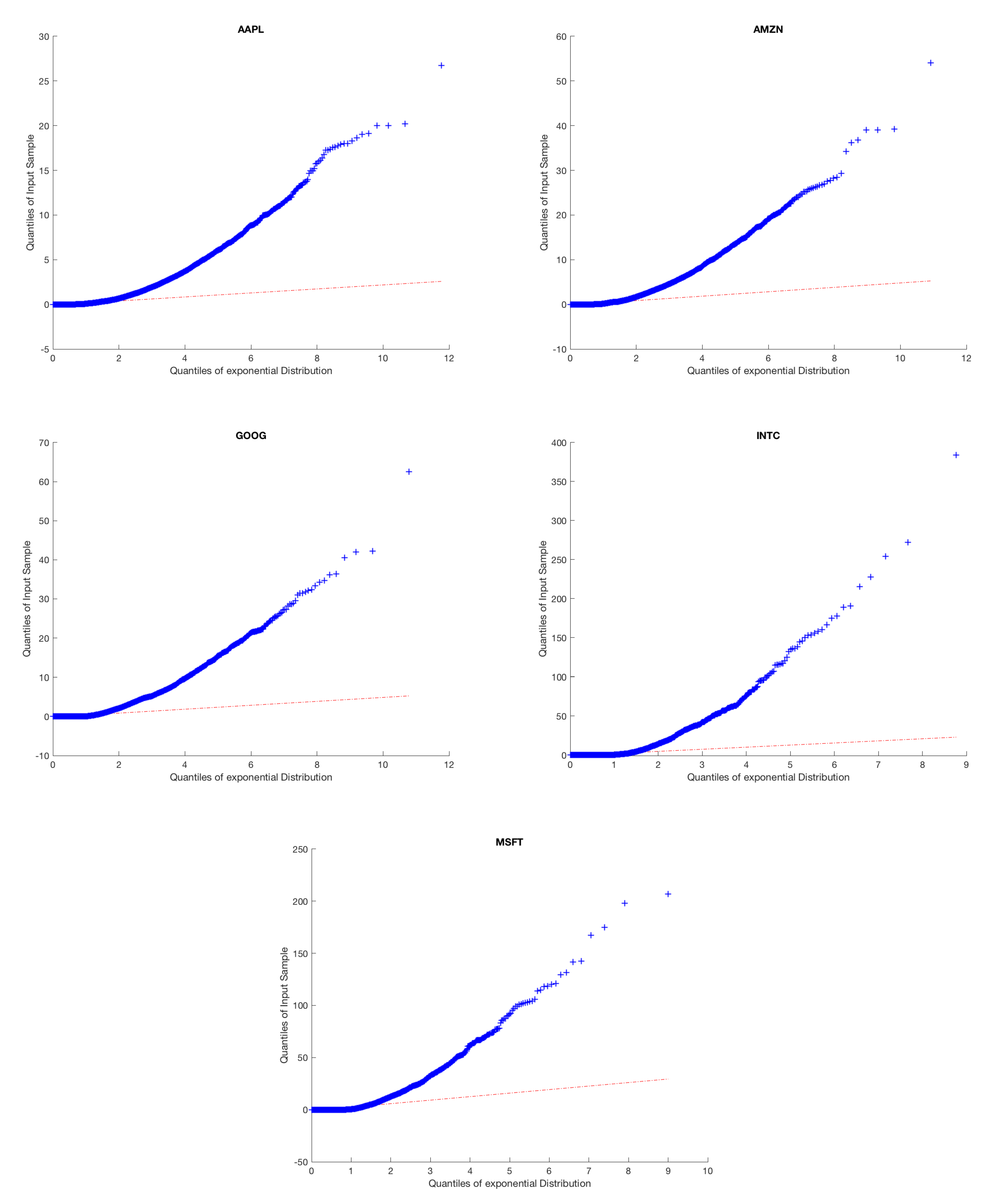
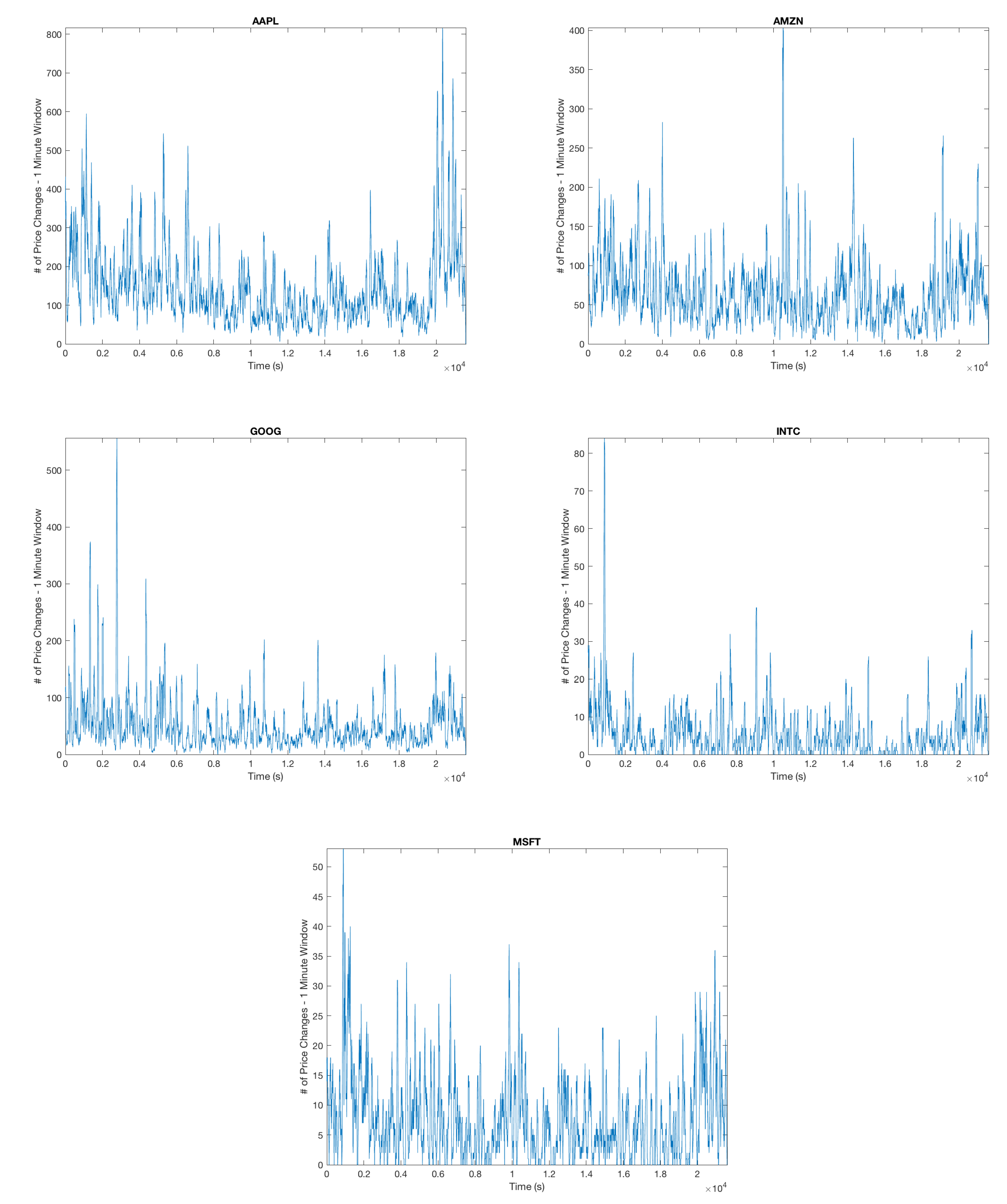
The high number of daily price changes motivates the idea that we can use asymptotic analysis in order to approximate long-run volatility using order flow by finding the diffusion limit of the price process. Because we do not want to include opening and closing auctions, we omit the first and last fifteen minutes of our data. We motivate the arrival process by analyzing the inter-arrival times and clustering to ensure the arrival process is not Poisson and exhibits the characteristics of a Hawkes Process. This is illustrated in Figure 1 and Figure 2.
Furthermore, the relationship between our diffusion coefficient and arrival process is limited to the expected number of arrivals on a unit interval. This implies that results for a simple exponential model can be easily generalized to a nonlinear one. This makes it possible to work with a simplified model for our Hawkes process, which is still rich enough to capture our observations. Keeping this in mind, we restrict ourselves to an exponential kernel and estimate parameters using an MLE Laub et al. (2015). We provide these estimates in Table 2 and compare the empirical expected number of arrivals and compare with the MLE estimate in Table 3.
Obviously, the MLE method accurately estimates the expected number of arrivals on the unit interval. This means we can confidently say for our data that our parameters will work reasonably with our models. We provide the estimated parameters in Table 2. We note that the novelty of the empirical results here compared with He and Swishchuk (2019) lies not only in the different stocks but also in considering the nonlinear Hawkes process as the model for a stock price.
Now that we have approximated the underlying arrival process, we quickly review our process for obtaining our empirical results:
- (1)
- Estimate the parameters of the arrival process using particle swarm optimization to maximize the negative loglikelihood function, as above.
- (2)
- Model the price change caused by an event using an -state Markov chain, with probabilities estimated by the relative frequencies
- (3)
- Use the diffusion limits determined previously to calculate the theoretical volatility and compare against what is observed
4.2. Compound Hawkes Process with Dependent ORders (CHPDO)
We first consider a compound Hawkes process with dependent orders defined in Definition 10, namely
where is a continuous-time two state Markov chain, is of fixed size and is the number of mid-price movements up to time t described by a Hawkes process.
We have opted to study the mid-price changes of our model. Thus, can be computed by averaging the best bid and ask price. Noting that the price is recorded in cents, the smallest possible jump in the mid-price is a half a cent, which we will use as . Furthermore, in order to estimate the transition matrix for the Markov chain , we count the absolute frequencies of upward and downward price movements and from this calculate the relative frequencies giving an estimate for and , which represent the conditional probabilities of an up/down movement given an up/down movement. Later, we will consider several different sizes of mid-price movements and will work with the convention that each movement will be assigned a state based off of its ordering in the reals. In this case, will be state one, and with be state two. This results in the transition matrix P given below:
After determining our parameters and transition probabilities, we calculate and in Table 4 together with and .
Provided these values, the asymptotic method from Section 3 and its Corollaries can be used to study the link between order flow in our model and price volatility. The estimated volatility of price changes is expressed in terms of parameters describing arrival rate of limit orders. Allowing us to test our claim that our model accurately describes the mid-price process. We recall that the mid-price , and the following diffusion limit
If the data satisfy our proposed model, then, after considering large windows of time (5 min, 10 min, 20 min), we would expect to see the empirical and theoretical standard deviations to follow each other closely. To test this, we compare the equivalent process, constructed by multiplying the LHS and RHS by . Then, cutting our data into disjoint windows of size n, specifically with and by setting the left bound as our starting time, we can calculate for each individual window and give a generalized formula for this below:
This gives a collection of values over which we compute the standard deviation. If our model is accurate, we would would expect that
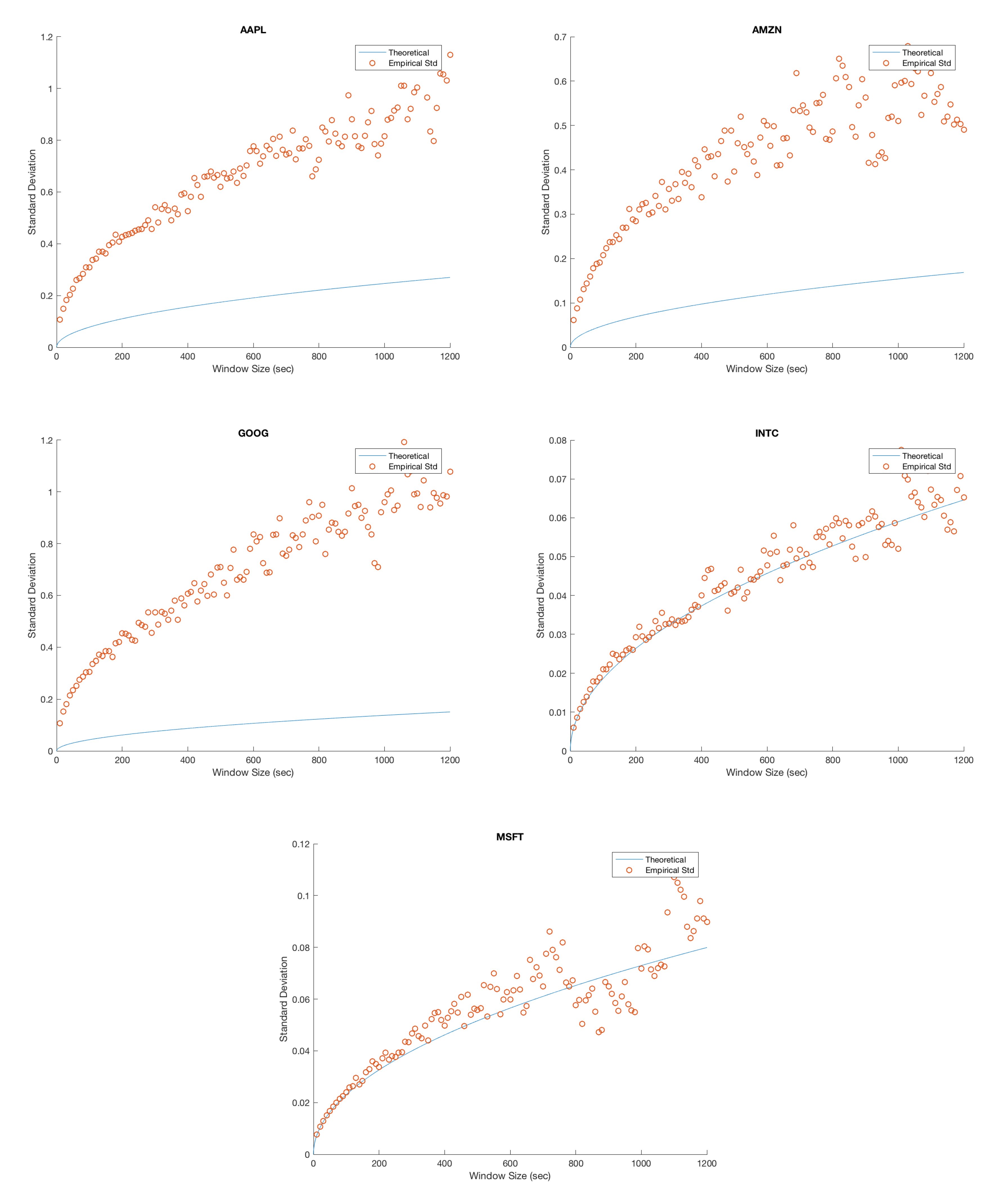
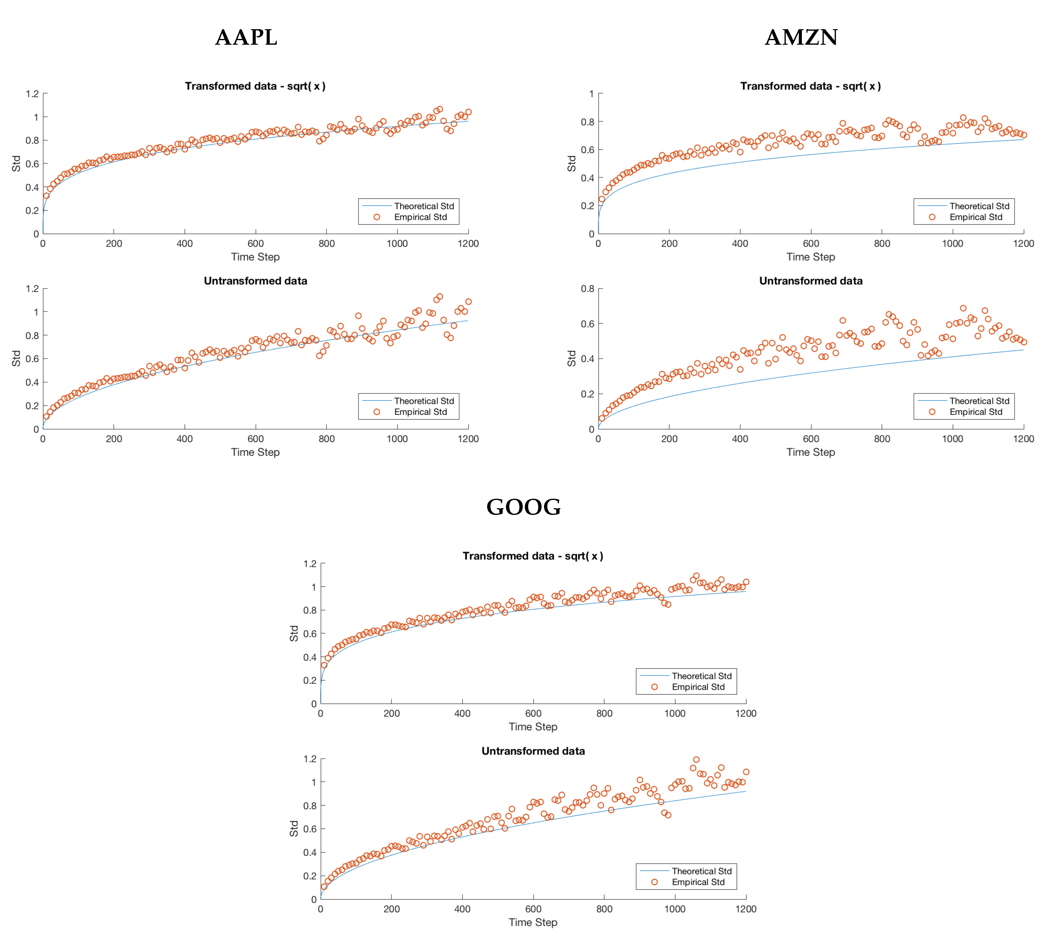
We plot the empirical standard deviation against the theoretical one for various window sizes starting at 10 s and increasing in steps of 10 s until we reach 20 min; this is illustrated in Figure 3.
Several important remarks should be made at this point. It is clear that, while the model accurately predicts the overall trend for MSFT and INTC, we severely underestimate the variability in the mid-price process for APPL, AMZN and GOOG. Furthermore, as the window size increases, the overall spread in the data increases. We attribute this to the decreasing sample size imposed on us as we increase the window size. For example, when we consider a 20 min window, we can only construct 27 disjoint windows in the 9 h trading day forcing us to deal with the problem of predicting a ’population’ standard deviation from a increasingly small sample. We remedy this by using a variance stabilizing transformation in later sections. Specifically, a popular method for a Poisson process is to take the square root of our empirical and theoretical standard deviations. This makes it possible to qualitatively view the overall trend in the data, gaining a clearer idea of goodness of fit from there.
4.3. General Compound Hawkes Process with Two Dependent Orders
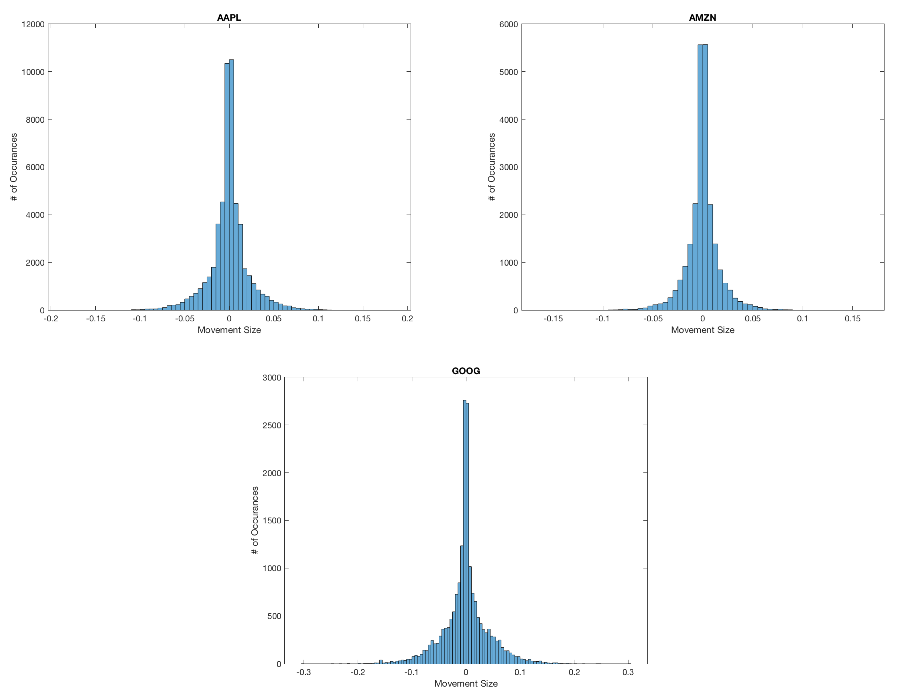
As of now, we have considered a fixed related to the trading tick size. However, if we consider the mid-price changes for APPL, AMZN and GOOG the assumption of a fixed tick size is violated. In fact, we observe that approximately 61%, 53% and 71% of all mid-price changes are larger than half a tick size, which is opposed to what we observe for MSFT and INTC where all mid-price changes occur at the half tick size, we illustrate this for AAPL, AMZN and GOOG in Figure 4.
It is clear in Figure 4 that additional considerations need to be made. A simple way to include the variability in mid-price movements in our model is to introduce as described in Definition 9. It is of course necessary to determine the values of for each state of our Markov chain. A naive method is to take the mean of the downward and upward mid-price movements and assign them to and , respectively. We provide these values in Table 5.
In this step, we have only endeavoured to better realize the actual price movements in our data. Therefore, when we observe a downward mid-price movement, we continue to assign it to state one and similarly for an upward price movement we continue to assign it to state two. It follows that our transition matrix will remain the same. Then, using these new state values, we recalculate and , providing them in Table 6. The effect of these changes is investigated in Figure 5. Note that in Figure 5 we have used the variance stabilizing transformation discussed earlier in order to better visualize the overall trend in our data.
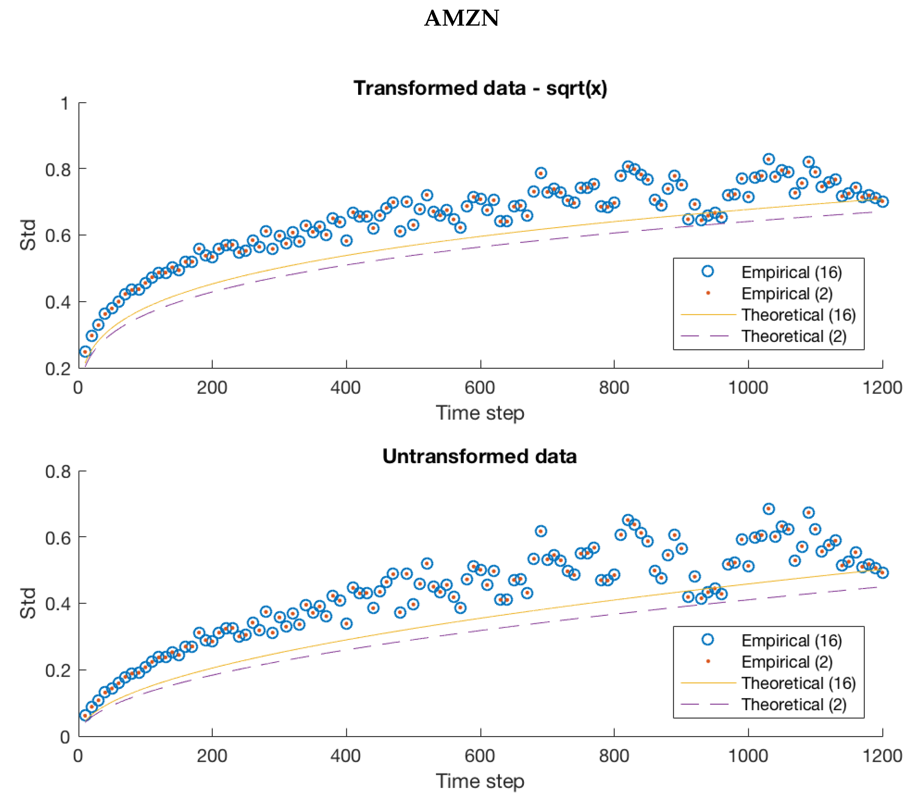
Notice that there is a significant qualitative improvement in the fits for AAPL and GOOG in Figure 5, but the variability in mid-price movements for AMZN is still clearly underestimated by our model. The unexplained variance may be captured by investigating an -state Markov chain since the additional transition probabilities could explain the variability missing in the 2-state case.
4.4. General Compound Hawkes Process with Dependent Orders
We recall the -state model described in Definition 8. The immediate question becomes how best to choose the state values. We modify the quantile based approach from Swishchuk et al. (2017). After calculating the mid-price changes, we separate the data into upward and downward price movements. Then, we calculate evenly distributed quantiles for both data sets. Depending on the data, several quantiles may be identical, we reject any duplicates. We thus obtain a list of bounds which we complete by adding the minimum observed value if necessary.
To determine the state values , we take the average of all mid-price changes located between two neighbouring boundary values. Furthermore, we assign a mid-price change to state i if it is greater than or equal to the th boundary and strictly less than the ith boundary. An exception is made for the largest upper bound where equality is permitted at both ends.
As we could not capture the full variability of mid-price changes for AMZN in the previous method, we investigate it for this case. Furthermore, for tractability, we only consider 14 boundary values from which we obtain a 12-state Markov chain. Instead of providing the transition matrix, we provide the ergodic probabilities for the transition matrix and the associated states in Table 7.
In order to compare the two state and -state approaches, we first take a qualitative approach and plot the two theoretical and empirical standard deviations against each other in Figure 6. When we compare the mean squared residuals, the 2-state model discussed before has mean squared error while our 12-state Markov chain brings that down to . Considering an even larger Markov chain with 24-states, we are only able to obtain a meager improvement to , suggesting that there is some underlying variance in the mid-price process not captured by our model. We investigate these more quantitative measures in the following subsection. First, comparing the models against a numerical best fit, and then investigating the mean squared error, we gain a better quantitative understanding of the overall improvement obtained from each model increasing the number of quantiles. While we do not propose a method for selecting an -state model in general, a possible piece of criteria is to halt when there is no appreciable gain in the MSE for more information (see Swishchuk et al. 2017, p. 17). In light of this, in the following section, we use k-fold cross-validation to make a determination.
5. Quantitative Analysis
While our model does visually appear to fit the expected variability in four of the five cases, it still fails to capture the complete dynamics of mid-price changes seen in our AMZN data. We investigate the mean square error of our models with a varying number of quantiles in Table 8. This gives a good indication as to whether the -state model is a better fit for our data. If we look closely at AAPL and GOOG, we see that the -state case can still improve our results from the 2-state case. For AAPL, we constructed a 17-state Markov chain by taking 16 quantiles on the downward movements and 16 quantiles upward movements. This resulted in a mean squared error of that is approximately a 28% improvement to the 2-state case where the mean squared error was . Even more extreme, using a 25-state Markov chain for GOOG which was constructed similarly, we observed a mean squared error of , which is a 60% improvement from the 2-state case with a mean squared error of . We conclude with Table 8, which provides the mean residuals for AAPL, AMZN and GOOG with several Markov chains constructed from various numbers of quantiles. We also include mean residuals for INTC and MSFT for comparison.
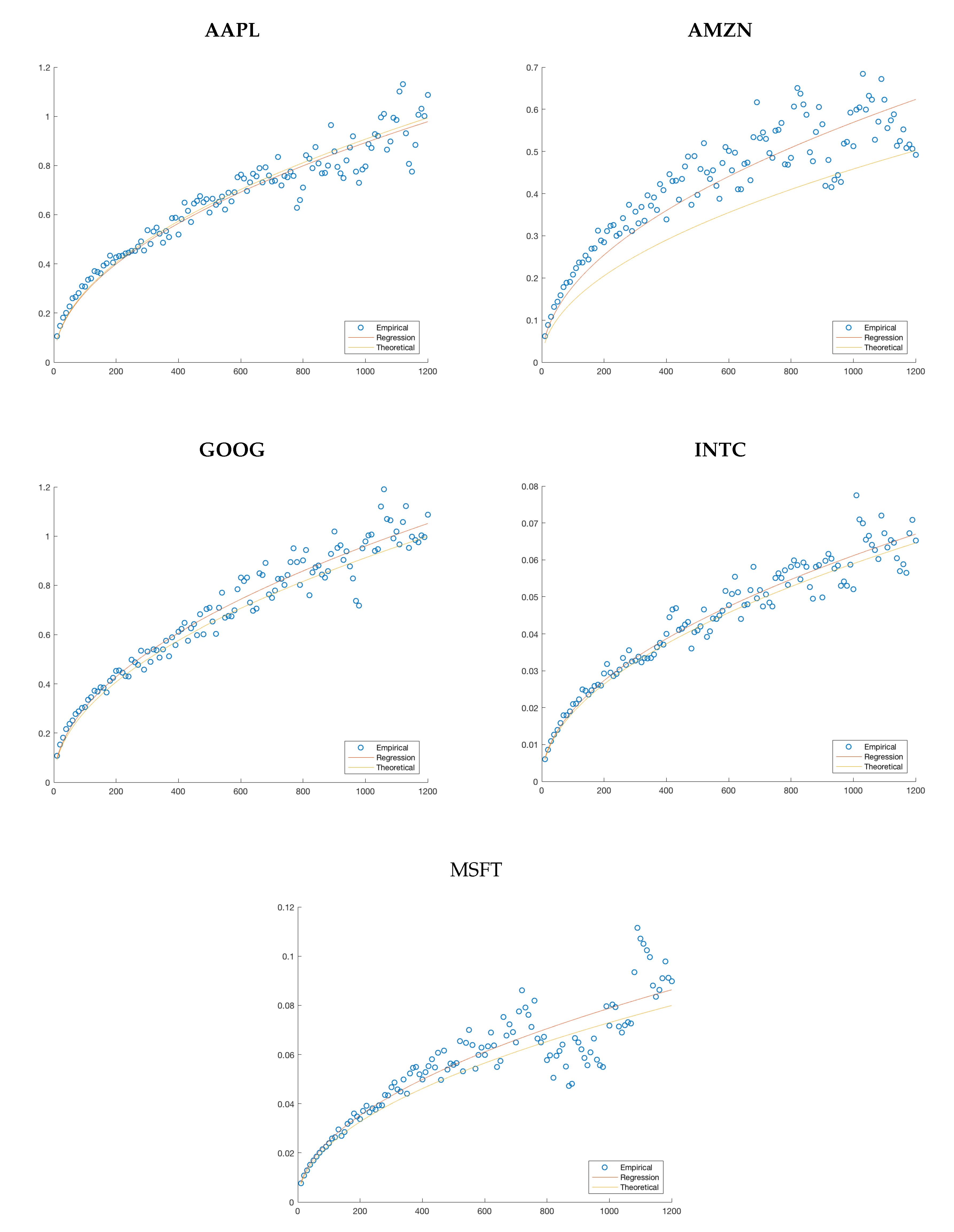
Another quantitative measure of our fit would be to compare them to the one which best minimizes the residuals. Notice that each of our models assumes that the standard deviation proportionally to the square root of the time step. Therefore, we can estimate the best possible coefficient by minimizing -norm or equivalently the mean squared error. We provide plots of these hypothetical best fits against the empirical data and theoretical fits in Figure 7. We also provide the coefficients for the theoretical fits and regression in Table 9 in order to have a more quantitative comparison. They are calculated using least-square regression.
We notice that in each case the errors are close to, or under five percent, with AMZN being the biggest offender. This is consistent with the discussion provided throughout our analysis and highlights the general applicability of our model.
Cross-Validation
We conclude this subsection using a method similar to k-fold cross-validation for model selection. Generally, the data are shuffled randomly and then partitioned into k sets of approximately equal size. From these k sets, one is selected for testing the model while the remaining are kept for training it. For our data, we are unable to perform this shuffling as there is an important ordering imposed by the arrival times. Fortunately, since we are considering high-frequency models for the mid-price changes, we expect a minimal amount of correlation in the volatility of the price process over large windows of time. Therefore, dividing the data into twelve 30 min windows selecting them one at a time should still be meaningful.
The training data will need to be glued back together after the thirty-minute window is removed. This is done by assuming the events never occurred. We provide an example below for how one would remove the second thirty-minute window in Table 10 and Table 11.
This introduces a small error into the arrival times, but only at a single point in a data set of several thousand arrival times. Had we randomly removed points, or shuffled the data, we could introduce many errors which could significantly change the underlying arrival process. At this point, we perform the same fitting procedure on the training data and after the fitting is completed, we can compute the empirical standard deviations on the testing data to obtain a mean squared error. This determines how well the model was able to predict the training data, calculating this for each window of time and averaging provides a score for how well the model was able to make predictions.
We recall that, for MSFT and INTC, the only observed prices changes were a single tick, and it is not possible to outperform the original CHPDO model. Instead, we consider AAPL, AMZN and GOOG calculating scores for CHPDO, GCHP2SDO and various GCHPnSDO models. Specifically the set of GCHPnSDO models are constructed using the quantile method, allowing for 2–14 quantiles. This was chosen only to make the recording more tractable; the resulting scores are provided in Table 12.
Overall, there is a meaningful gain in performance for the -state models, especially when we take into account the previous discussion. The cross-validation we’ve performed provides a reasonable criteria for model rejection, similar to when we stop observing appreciable gains in the mean squared error. From our analysis, the best model would be one constructed from 4–7 quantiles, depending on the stock of interest.
6. Conclusions and Future Work
Overall, the -state model outperforms the others when the number of states is kept small. It generates fits for four out of the five datasets that are reasonable and providing reductions in the mean squared error by upwards of 25%. While not able to capture the full dynamics observed in AMZN, it appears to be a strong candidate for a simple model of price dynamics observed in our data. Further investigation would be necessary to determine what causes the additional volatility observed in AMZN, and potentially implement a more robust model which captures this. The potential users of our models are practitioners working in the financial industry who wish to implement our results in high-frequency and algorithmic trading combined with their industrial knowledge.
Author Contributions
Both authors have contributed equally to the paper. All authors have read and agreed to the published version of the manuscript.
Funding
This research was funded by NSERC Grant No. RT732266.
Conflicts of Interest
The authors declare no conflict of interest.
References
- Azizpour, Shahriar, Kay Giesecke, and Gustavo Schwenkler. 2018. Exploring the sources of default clustering. Journal of Financial Economics 129: 154–83. [Google Scholar] [CrossRef]
- Aït-Sahalia, Yacine, Julio Cacho-Diaz, and Roger J.A. Laeven. 2015. Modeling financial contagion using mutually exciting jump processes. Journal of Financial Economics 117: 585–606. [Google Scholar] [CrossRef] [Green Version]
- Bacry, Emmanuel, Sylvain Delattre, Marc Hoffmann, and Jean-François Muzy. 2011. Modeling microstructure noise with mutually exciting point processes. arXiv arXiv:1101.3422. [Google Scholar]
- Bacry, Emmanuel, Iacopo Mastromatteo, and Jean-François Muzy. 2015. Hawkes processes in finance. arXiv arXiv:1502.04592. [Google Scholar] [CrossRef]
- Bartlett, Maurice Stevenson. 1963. The spectral analysis of point processes. Journal of the Royal Statistical Society. Series B (Methodological) 25: 264–296. [Google Scholar] [CrossRef]
- Bauwens, Luc, and Nikolaus Hautsch. 2009. Modelling Financial High Frequency Data Using Point Processes. Berlin/Heidelberg: Springer, pp. 953–79. [Google Scholar] [CrossRef] [Green Version]
- Bowsher, Clive G. 2007. Modelling security market events in continuous time: Intensity based, multivariate point process models. Journal of Econometrics 141: 876–912. [Google Scholar] [CrossRef] [Green Version]
- Brémaud, Pierre, and Laurent Massoulié. 1996. Stability of nonlinear hawkes processes. The Annals of Probability 24: 1563–88. [Google Scholar] [CrossRef]
- Buffington, John, and Robert J. Elliott. 2002a. American options with regime switching. International Journal of Theoretical and Applied Finance 5: 497–514. [Google Scholar] [CrossRef]
- Buffington, John, and Robert J. Elliott. 2002b. Regime switching and european options. In Stochastic Theory and Control. Edited by B. Pasik-Duncan. Berlin/Heidelberg: Springer, pp. 73–82. [Google Scholar]
- Carstensen, Lisbeth. 2010. Hawkes Processes and Combinatiorial Transcriptional Regulation. København: Museum Tusculanum. [Google Scholar]
- Cartea, Álvaro, Sebastian Jaimungal, and José Penalva. 2015. Algorithmic and High-Frequency Trading. Cambridge: Cambridge University Press. [Google Scholar]
- Cartea, Álvaro, Sebastian Jaimungal, and Jason Ricci. 2014. Buy low, sell high: A high frequency trading perspective. SIAM Journal on Financial Mathematics 5: 415–44. [Google Scholar] [CrossRef]
- Chávez-Casillas, Jonathan A., Robert J. Elliott, Bruno Rémillard, and Anatoliy V. Swishchuk. 2019. A level-1 limit order book with time dependent arrival rates. Methodology and Computing in Applied Probability 21: 699–719. [Google Scholar] [CrossRef] [Green Version]
- Chavez-Demoulin, Valérie, and J. A. McGill. 2012. High-frequency financial data modeling using hawkes processes. Journal of Banking & Finance 36: 3415–26. [Google Scholar]
- Cohen, Samuel N., and Robert J. Elliott. 2013. Filters and smoothers for self-exciting Markov modulated counting processes. arXiv arXiv:1311.6257. [Google Scholar]
- Cox, David R. 1955. Some statistical methods connected with series of events. Journal of the Royal Statistical Society Series B (Methodological) 17: 129–64. [Google Scholar] [CrossRef]
- Daley, Daryl J., and David Vere-Jones. 2003. An Introduction to The Theory of Point Processes: Volume I: Elementary Theory and Methods. Berlin/Heidelberg: Springer Science & Business Media. [Google Scholar]
- Dassios, Angelos, and Hongbiao Zhao. 2011. A dynamic contagion process. Advances in Applied Probability 43: 814–46. [Google Scholar] [CrossRef]
- Embrechts, Paul, Thomas Liniger, and Lu Lin. 2011. Multivariate hawkes processes: An application to financial data. Journal of Applied Probability 48A: 367–78. [Google Scholar] [CrossRef]
- Engle, Robert F., and Jeffrey R. Russell. 1998. Autoregressive conditional duration: A new model for irregularly spaced transaction data. Econometrica 1998: 1127–62. [Google Scholar] [CrossRef]
- Errais, Eymen, Kay Giesecke, and Lisa R. Goldberg. 2010. Affine point processes and portfolio credit risk. SIAM Journal on Financial Mathematics 1: 642–65. [Google Scholar] [CrossRef] [Green Version]
- Filimonov, Vladimir, David Bicchetti, Nicolas Maystre, and Didier Sornette. 2014. Quantification of the high level of endogeneity and of structural regime shifts in commodity markets. Journal of International Money and Finance 42: 174–92. [Google Scholar] [CrossRef] [Green Version]
- Filimonov, Vladimir, and Didier Sornette. 2012. Quantifying reflexivity in financial markets: Toward a prediction of flash crashes. Physical Review E 85: 056108. [Google Scholar] [CrossRef] [Green Version]
- Getoor, Ronald Kay. 1967. Review: A. v. skorokhod, studies in the theory of random processes. The Annals of Mathematical Statistics 38: 287. [Google Scholar] [CrossRef]
- Hasbrouck, Joel. 1999. Trading Fast and Slow: Security Market Events in Real Time. Leonard N. Stern School Finance Department Working Paper Seires 99-012; New York: New York University, Leonard N. Stern School of Business. [Google Scholar]
- Hawkes, Alan G. 1971. Spectra of some self-exciting and mutually exciting point processes. Biometrika 58: 83–90. [Google Scholar] [CrossRef]
- Hawkes, Alan G., and David Oakes. 1974. A cluster process representation of a self-exciting process. Journal of Applied Probability 11: 493–503. [Google Scholar] [CrossRef]
- He, Qiyue, and Anatoliy Swishchuk. 2019. Quantitative and comparative analyses of limit order books with general compound hawkes processes. Risks 7: 110. [Google Scholar] [CrossRef] [Green Version]
- Hewlett, Patrick. 2006. Clustering of Order Arrivals, Price Impact and Trade Path Optimisation. Available online: https://pdfs.semanticscholar.org/7a5c/ec408693f3f2ce2134374ee007b7c6b4973d.pdf (accessed on 12 March 2020).
- Large, Jeremy. 2007. Measuring the resiliency of an electronic limit order book. Journal of Financial Markets 10: 1–25. [Google Scholar] [CrossRef] [Green Version]
- Laub, Patrick J., Thomas Taimre, and Philip K. Pollett. 2015. Hawkes processes. arXiv arXiv:1507.02822. [Google Scholar]
- Lewis, Peter A. W. 1964. A branching poisson process model for the analysis of computer failure patterns. Journal of the Royal Statistical Society: Series B (Methodological) 26: 398–441. [Google Scholar] [CrossRef]
- Liniger, Thomas Josef. 2009. Multivariate Hawkes Processes. Ph.D. Thesis, ETH Zurich, Zurich, Switzerland. [Google Scholar]
- Mehrdad, Behzad, and Lingjiong Zhu. 2014. On the Hawkes Process with Different Exciting Functions. arXiv arXiv:1403.0994. [Google Scholar]
- Mohler, George O., M. B. Short, P. J. Brantingham, F. P. Schoenberg, and G. E. Tita. 2011. Self-exciting point process modeling of crime. Journal of the American Statistical Association 106: 100–8. [Google Scholar] [CrossRef]
- Norris, James R. 1997. Markov Chains. Cambridge Series in Statistical and Probabilistic Mathematics; Cambridge: Cambridge University Press. [Google Scholar] [CrossRef]
- Ogata, Yosihiko. 1988. Statistical models for earthquake occurrences and residual analysis for point processes. Journal of the American Statistical Association 83: 9–27. [Google Scholar] [CrossRef]
- Swishchuk, Anatoliy. 2017. Risk Model Based on General Compound Hawkes Process. arXiv arXiv:1706.09038. [Google Scholar] [CrossRef] [Green Version]
- Swishchuk, Anatoliy, Tyler Hofmeister, Katharina Cera, and Julia Schimidt. 2017. General semi-markov model for limit order books. International Journal of Theoretical and Applied Finance 20: 1750019. [Google Scholar] [CrossRef]
- Swishchuk, Anatoliy, and Aiden Huffman. 2018. General Compound Hawkes Processes in Limit Order Books. arXiv arXiv:1812.02298. [Google Scholar] [CrossRef] [Green Version]
- Swishchuk, Anatoliy, Bruno Remillard, Robert Elliott, and Jonathan Chavez-Casillas. 2019. Compound hawkes processes in limit order books. In Financial Mathematics, Volatility and Covariance Modelling. Edited by Julien Chevallier, Stéphane Goutte, David Guerreiro, Sophie Saglio and Bilel Sanhaji. Abingdon upon Thames: Routledge Advances in Applied Financial Econometrics, pp. 191–214. [Google Scholar]
- Swishchuk, Anatoliy, and Nelson Vadori. 2017. A semi-markovian modeling of limit order markets. SIAM Journal on Financial Mathematics 8: 240–73. [Google Scholar] [CrossRef] [Green Version]
- Vadori, Nelson, and Anatoliy Swishchuk. 2015. Strong law of large numbers and central limit theorems for functionals of inhomogeneous semi-markov processes. Stochastic Analysis and Applications 33: 213–43. [Google Scholar] [CrossRef]
- Vinkovskaya, Ekaterina. 2014. A Point Process Model for the Dynamics of Limit Order Books. New York: Columbia University. [Google Scholar] [CrossRef]
- Zheng, Ban, François Roueff, and Frédéric Abergel. 2013. Ergodicity and scaling limit of a constrained multivariate Hawkes process. arXiv arXiv:1301.5007. [Google Scholar] [CrossRef] [Green Version]
Figure 1.
Above, we provide a quantile-quantile plot of our empirical inter-arrival times against a Poisson process for each of the five stocks. We see that the inter-arrival data does not fit the expected curve, providing evidence that the underlying arrival process is not Poisson.
Figure 1.
Above, we provide a quantile-quantile plot of our empirical inter-arrival times against a Poisson process for each of the five stocks. We see that the inter-arrival data does not fit the expected curve, providing evidence that the underlying arrival process is not Poisson.

Figure 2.
Each plot shows the number of arrivals for a moving one minute window. From this, we can conclude that there is a significant amount of clustering in the arrival of mid-price changes, motivating the Hawkes model of our arrival process.
Figure 2.
Each plot shows the number of arrivals for a moving one minute window. From this, we can conclude that there is a significant amount of clustering in the arrival of mid-price changes, motivating the Hawkes model of our arrival process.

Figure 3.
Each figure compares the empirical standard deviation for a fixed window size to the theoretical standard deviation. We have plotted an empirical standard deviation for all n from 10 s to 20 min in step sizes of 10 s. Each empirical standard deviation corresponds to a single point in the scatter plot, and the plotted curve corresponds to the predicted theoretical value.

Figure 4.
We can see clearly that the change in the mid-price is often larger than a half tick. These mid-price changes make up a significant portion of the actual data, contradicting the assumption needed for the CHPDO model that the mid-price changes occur on average at a half tick size.
Figure 4.
We can see clearly that the change in the mid-price is often larger than a half tick. These mid-price changes make up a significant portion of the actual data, contradicting the assumption needed for the CHPDO model that the mid-price changes occur on average at a half tick size.

Figure 5.
A comparison of the empirical standard deviation for a fixed window size n to the theoretical standard deviation for AAPL, AMZN and GOOG using the 2-state dependent order model. We have plotted the empirical standard deviation for all n from 10 s to 20 min in step sizes of 10 s. Each empirical standard deviation corresponds to a single point in the scatter plot and the plotted curve corresponds to the predicted theoretical value. Visually, there is a significant improvement for all stocks, although the theoretical standard deviation for AMZN is still underestimating the empirical variability.

Figure 6.
We consider the N-state model for AMZN discussed previously in the paper. While there is a slight improvement against the original fit, the model still struggles to perfectly predict the variability in the mid-price changes of our data.
Figure 6.
We consider the N-state model for AMZN discussed previously in the paper. While there is a slight improvement against the original fit, the model still struggles to perfectly predict the variability in the mid-price changes of our data.

Figure 7.
A qualitative comparison of the regression to the theoretical model. For APPL, AMZN and GOOG, we have used a Markov chain generated from 16 quantiles taken on the upward movements and downward movements. For INTC and MSFT, we have taken the CHPDO coefficient since a different coefficient is not possible with the other models.


Table 1.
Stock liquidity of AAPL, AMZN, GOOG, MSFT, and INTC for 21 June 2012.
| Ticker | Avg # of Orders per 10 s | Price Changes in 1 Day |
|---|---|---|
| AAPL | 51 | 64,350 |
| AMZN | 25 | 27,557 |
| GOOG | 21 | 24,084 |
| MSFT | 173 | 3217 |
| INTC | 176 | 4060 |
Table 2.
Each parameter was estimated using a particle swarm optimization method in an attempt to globally optimize the negative log-likelihood function. The values for , and for each data set are as provided.
Table 2.
Each parameter was estimated using a particle swarm optimization method in an attempt to globally optimize the negative log-likelihood function. The values for , and for each data set are as provided.
| AAPL | 1.4683 | 1045.2676 | 2556.1844 |
| AMZN | 0.6443 | 653.7524 | 1556.1702 |
| GOOG | 0.4985 | 865.8553 | 1980.4409 |
| MSFT | 0.0659 | 479.3482 | 908.0032 |
| INTC | 0.0471 | 399.6389 | 760.4991 |
Table 3.
Expected number of arrivals on a unit interval using estimated parameters from an MLE method is compared against the empirical arrivals.
Table 3.
Expected number of arrivals on a unit interval using estimated parameters from an MLE method is compared against the empirical arrivals.
| Emp. | MLE | |
|---|---|---|
| AAPL | 2.4840 | 2.4841 |
| AMZN | 1.1110 | 1.1110 |
| GOOG | 0.8857 | 0.8857 |
| MSFT | 0.1395 | 0.1396 |
| INTC | 0.0991 | 0.0992 |
Table 4.
Provided above are the values for , as well as the probabilities of an upward/downward movement given an upward/downward movement for each of the five stocks in question.
Table 4.
Provided above are the values for , as well as the probabilities of an upward/downward movement given an upward/downward movement for each of the five stocks in question.
| AAPL | 0.4956 | 0.4933 | 0.0049 | −1.1463 × 10 |
| AMZN | 0.4635 | 0.4576 | 0.0046 | −2.7373 × 10 |
| GOOG | 0.4769 | 0.4461 | 0.0046 | −1.4301 × 10 |
| MSFT | 0.6269 | 0.5827 | 0.0062 | −2.7956 × 10 |
| INTC | 0.6106 | 0.5588 | 0.0059 | −3.1185 × 10 |
Table 5.
is the average of the upward or downward mid-price movements. Following our previous convention, the first state will be associated with the mean of all downward mid-price movements and the second state will be associated with the mean of all upward mid-price movements.
Table 5.
is the average of the upward or downward mid-price movements. Following our previous convention, the first state will be associated with the mean of all downward mid-price movements and the second state will be associated with the mean of all upward mid-price movements.
| AAPL | −0.0172 | 0.0170 |
| AMZN | −0.0134 | 0.0133 |
| GOOG | −0.0302 | 0.0308 |
Table 6.
Above, we have the values for , as well as the probabilities of an upwards/downwards movement, given an upwards/downwards movement for the three stocks of interest.
Table 6.
Above, we have the values for , as well as the probabilities of an upwards/downwards movement, given an upwards/downwards movement for the three stocks of interest.
| AAPL | 0.4956 | 0.4933 | 0.0169 | −1.5624 × 10 |
| AMZN | 0.4635 | 0.4576 | 0.0123 | −1.0475 × 10 |
| GOOG | 0.4769 | 0.4461 | 0.0282 | −5.5095 × 10 |
Table 7.
Above, we have provided the state, associated ergodic probabilities and state values for AMZN, given a 12-state Markov chain that was obtained from choosing a 16 quantile method.
Table 7.
Above, we have provided the state, associated ergodic probabilities and state values for AMZN, given a 12-state Markov chain that was obtained from choosing a 16 quantile method.
| AMZN | ||
|---|---|---|
| i | ||
| 1 | 0.0275 | −0.0524 |
| 2 | 0.0281 | −0.0318 |
| 3 | 0.0264 | −0.0250 |
| 4 | 0.0382 | −0.0200 |
| 5 | 0.0576 | −0.0150 |
| 6 | 0.3249 | −0.0064 |
| 7 | 0.2321 | 0.0050 |
| 8 | 0.0923 | 0.0100 |
| 9 | 0.0578 | 0.0150 |
| 10 | 0.0353 | 0.0200 |
| 11 | 0.0412 | 0.0271 |
| 12 | 0.0387 | 0.0476 |
Table 8.
We list the mean residuals for several Markov chains with varying numbers of states. These were generated using our modified quantile approach choosing to start with 2, 8, 16 or 32 quantiles. We see that, in general, the mean residual decreases to some lower limit where we can no longer perform any better. Recall that the only observed mid-price changes for INTC and MSFT were of a half tick size, and any increase in the number of quantiles will result in the same performance.
| CHPDO | 2 | 8 | 16 | 32 | |
|---|---|---|---|---|---|
| AAPL | 0.2679 | 0.0050 | 0.0036 | 0.0036 | 0.0036 |
| AMZN | 0.1122 | 0.0208 | 0.0131 | 0.0124 | 0.0123 |
| GOOG | 0.4036 | 0.0115 | 0.0048 | 0.0045 | 0.0047 |
| INTC | 1.7917 × 10 | 1.7917 × 10 | 1.7917 × 10 | 1.7917 × 10 | 1.7917 × 10 |
| MSFT | 1.0586 × 10 | 1.0586 × 10 | 1.0586 × 10 | 1.0586 × 10 | 1.0586 × 10 |
Table 9.
The coefficients calculated for AAPL, AMZN and GOOG are generated using a Markov chain created by 16 quantiles on the upward and downward movements, while the coefficients for INTC and MSFT are obtained from the CHPDO case.
Table 9.
The coefficients calculated for AAPL, AMZN and GOOG are generated using a Markov chain created by 16 quantiles on the upward and downward movements, while the coefficients for INTC and MSFT are obtained from the CHPDO case.
| Theoretical Coefficient | Regression Coefficient | Percent Error | |
|---|---|---|---|
| AAPL | 0.02868 | 0.02828 | 1.42% |
| AMZN | 0.01450 | 0.01831 | 20.8% |
| GOOG | 0.02883 | 0.03023 | 4.63% |
| INTC | 0.00186 | 0.00193 | 3.4% |
| MSFT | 0.00231 | 0.00246 | 6.4% |
Table 10.
An imagined sequence of price change events before the second thirty minute window has been removed.
Table 10.
An imagined sequence of price change events before the second thirty minute window has been removed.
| Time (s) | ⋯ | 1789 | 1795 | 1803 | ⋯ | 3193 | 3601 | 3608 | ⋯ |
| Event | ⋯ | n − 1 | n | n + 1 | ⋯ | n + k | n + k + 1 | n + k + 2 | ⋯ |
Table 11.
An imagined sequence of price change events after the second thirty minute window has been removed.
Table 11.
An imagined sequence of price change events after the second thirty minute window has been removed.
| Time (s) | ⋯ | 1789 | 1795 | 1801 | 1808 | ⋯ |
| Event | ⋯ | n − 1 | n | n + k + 1 | n + k + 2 | ⋯ |
Table 12.
A table of testing scores for various models. Computations were performed for up to the 40-quantile case for each stock, and this table represents a sample of that data. We note that the models stop obtaining appreciable performance gains at around 4–7 quantiles, fluctuating around the same scores.
| AAPL | AMZN | GOOG | |
|---|---|---|---|
| CHPDO | 0.0348 | 0.0142 | 0.0436 |
| GCHP2SDO | 0.0049 | 0.0048 | 0.0044 |
| 2-Quantiles | 0.0042 | 0.0041 | 0.0036 |
| 3-Quantiles | 0.0041 | 0.0042 | 0.0035 |
| 4-Quantiles | 0.0040 | 0.0040 | 0.0035 |
| 5-Quantiles | 4.0341 × 10 | 3.9878 × 10 | 3.4593 × 10 |
| 6-Quantiles | 4.0362 × 10 | 3.8971 × 10 | 3.4168 × 10 |
| 7-Quantiles | 4.0184 × 10 | 3.8971 × 10 | 3.3977 × 10 |
| 8-Quantiles | 4.0097 × 10 | 3.8656 × 10 | 3.3881 × 10 |
| 9-Quantiles | 4.0026 × 10 | 3.8124 × 10 | 3.3976 × 10 |
| 10-Quantiles | 3.9984 × 10 | 3.8124 × 10 | 3.425 × 10 |
| 11-Quantiles | 3.9971 × 10 | 3.81594 × 10 | 3.3867 × 10 |
| 12-Quantiles | 3.9826 × 10 | 3.81463 × 10 | 3.3906 × 10 |
| 13-Quantiles | 3.9804 × 10 | 3.81517 × 10 | 3.3562 × 10 |
| 14-Quantiles | 3.9725 × 10 | 3.81427 × 10 | 3.3549 × 10 |
© 2020 by the authors. Licensee MDPI, Basel, Switzerland. This article is an open access article distributed under the terms and conditions of the Creative Commons Attribution (CC BY) license (http://creativecommons.org/licenses/by/4.0/).
Share and Cite
MDPI and ACS Style
Swishchuk, A.; Huffman, A. General Compound Hawkes Processes in Limit Order Books. Risks 2020, 8, 28. https://0-doi-org.brum.beds.ac.uk/10.3390/risks8010028
AMA Style
Swishchuk A, Huffman A. General Compound Hawkes Processes in Limit Order Books. Risks. 2020; 8(1):28. https://0-doi-org.brum.beds.ac.uk/10.3390/risks8010028
Chicago/Turabian StyleSwishchuk, Anatoliy, and Aiden Huffman. 2020. "General Compound Hawkes Processes in Limit Order Books" Risks 8, no. 1: 28. https://0-doi-org.brum.beds.ac.uk/10.3390/risks8010028
Note that from the first issue of 2016, this journal uses article numbers instead of page numbers. See further details here.