Effect of Variance Swap in Hedging Volatility Risk

Abstract

This paper studies the effect of variance swap in hedging volatility risk under the mean-variance criterion. We consider two mean-variance portfolio selection problems under Heston’s stochastic volatility model. In the first problem, the financial market is complete and contains three primitive assets: a bank account, a stock and a variance swap, where the variance swap can be used to hedge against the volatility risk. In the second problem, only the bank account and the stock can be traded in the market, which is incomplete since the idiosyncratic volatility risk is unhedgeable. Under an exponential integrability assumption, we use a linear-quadratic control approach in conjunction with backward stochastic differential equations to solve the two problems. Efficient portfolio strategies and efficient frontiers are derived in closed-form and represented in terms of the unique solutions to backward stochastic differential equations. Numerical examples are provided to compare the solutions to the two problems. It is found that adding the variance swap in the portfolio can remarkably reduce the portfolio risk.

1. Introduction

It is widely recognized that the volatility of stocks evolves in a stochastic fashion rather than being constant or deterministic over time. Many empirical studies on stock options reveal that the implied volatility in option price data exhibit the so-called volatility smile/skew, which cannot be explained by the constant-volatility stock price models, say, the geometric Brownian motion model adopted in the Black and Scholes (1973) formula. Tremendous effort has been made to articulate this issue, and various stochastic volatility models have been developed to capture the volatility smile/skew as observed in the market. See, for example, French et al. (1987), Hull and White (1987), Wiggins (1987), Stein and Stein (1991), and Heston (1993). Among these stochastic volatility models, the most commonly used is certainly Heston’s model (Heston 1993). Indeed, the variance process described by Heston’s model follows a single-factor square-root process with mean-reversion, i.e., a Cox-Ingersoll-Ross (CIR) process, which is mathematically tractable even when the instantaneous volatility/variance is assumed to be correlated with the stock price.

The early research of Heston’s model focuses on option pricing under this model. Recently, there has been emerging interest in portfolio selection problems under Heston’s model as well as other stochastic volatility models. One direction of research is on maximizing the expected utility from investment and consumption. Kraft (2005) investigates a utility maximization problem and provides an explicit solution of the problem under specific conditions on model parameters. With the help of a martingale criterion, Kallsen and Muhle-Karbe (2010) derive explicit solutions for a power utility maximization problem in a number of affine-form stochastic volatility models. Zeng and Taksar (2013) study an optimal portfolio selection problem under a general stochastic volatility model and obtain closed-form solutions for Heston’s model under more relaxed assumptions. Other relevant works along this direction include, for example, Zariphopoulou (2001), Fleming and Hernández-Hernández (2003), Liu et al. (2003), and Chacko and Viceira (2005). Another direction of research explores the mean-variance hedging, that is, the problem of approximating a given final payoff by a self-financing trading strategy so as to minimize the mean-squared error. Preceding works include Laurent and Pham (1999), Biagini et al. (2000), Hobson (2004), Černý and Kallsen (2008), to name but only a few.

Although portfolio selection problems under Heston’s model have been extensively studied, most existing works concentrate on portfolio selection under the utility-maximization or the mean-variance hedging criteria and few attention has been paid to that under Markowitz (1952)’s mean-variance paradigm. In fact, Markowitz (1952)’s mean-variance criterion and Merton (1969, 1971)’s utility-maximization criterion are both considered precursors of modern portfolio optimization theory, and, to some degree, they are of equal importance in the field. On the other hand, the history of the mean-variance portfolio selection is much longer than that of the mean-variance hedging. In Markowitz (1952), the mean-variance portfolio selection problem is proposed in a single-period discrete-time setting. Using some delicate embedding techniques, Zhou and Li (2000) apply the linear-quadratic (LQ) control theory to solve a continuous-time mean-variance portfolio selection problem analytically. Subsequently, Lim and Zhou (2002), Lim (2004) and Lim (2005) study mean-variance portfolio selection problems with random parameters by using the LQ control and backward stochastic differential equations (BSDEs). At first glance, one may consider nesting the mean-variance portfolio selection problem under Heston’s model in Lim and Zhou’s framework. However, this is impossible since the variance process in Heston’s model is unbounded, which violates the boundedness assumption of model parameters in Lim and Zhou’s framework. In fact, a class of nonlinear BSDEs is used to solve mean-variance problems, and this class is termed backward stochastic differential Riccati equations (BSREs). Because there are no general results for BSREs with unbounded coefficients, it is challenging to use BSREs to solve mean-variance problems under Heston’s model. This attracts recent attention to studying mean-variance portfolio selection problems with unbounded random coefficients. See Chiu and Wong (2011, 2014), Shen et al. (2014), Shen and Zeng (2015), Shen (2015), Li et al. (2018), etc.

The focus of the the current paper is on demonstrating that volatility derivatives (e.g., variance swap) is effective tool to manage volatility risk when the stock price dynamics is only partially correlated with the stochastic volatility dynamics. Particularly, the advantage of using variance swap contracts is that there is no cost of entering into these contracts since swaps are worth zero at issuance. Compared with other volatility derivatives, e.g., variance and volatility options, variance swaps provide non-directional exposure to volatility risk, which then reduces the need for delta-hedging residual volatility risk.

To investigate the effect of variance swaps in hedging volatility risk, in this paper we consider two dynamic mean-variance portfolio selection problems under Heston’s stochastic volatility model in a complete market and an incomplete market, respectively. More specifically, we assume that a bank account, a stock and a variance swap are traded in the complete market and that only the bank account and the stock are traded in the incomplete market. The variance process of the stock is described by Heston’s model and is correlated with the stock price process. Throughout this paper, we make a standing assumption that the variance process/the market price of risk process is exponentially integrable. We employ a combined LQ control and BSDE approach to solve the two problems. To address the issue in the solvability of BSREs with unbounded coefficients, we use measure change techniques and study several transformed BSDEs under equivalent probability measures first. Based on the exponential-integrability assumption, Girsanov’s theorem, Hölder’s inequality and the one-to-one correspondence relationships between the solutions to the original BSREs and the transformed BSDEs, the uniqueness and existence of solutions to the original BSREs are proved under the real-world probability measure. Due to the Markovian structure, the unique solutions to these BSREs can be represented by the solutions to some Riccati-type ordinary differential equations (ODEs). With the unique solutions to related BSREs, a straightforward application of the LQ control theory leads to the explicit expressions of the efficient portfolio strategies and the efficient frontiers immediately. To examine the differences of the two problems and the effect of adding the variance swap in the portfolio, we provide numerical examples of the efficient frontiers with different parameter values in the complete and the incomplete markets. It is shown that the variance swap can reduce the overall risk of the terminal wealth through hedging against the volatility risk. In addition, we verify that if the stock price and variance processes are perfectly correlated, the complete market and the incomplete one are indistinguishable. Therefore, the variance swap is an effective tool to hedge idiosyncratic volatility risk.

On technical side, this paper somehow extends Shen (2015) and Shen and Zeng (2015) to cater for the current setting. Shen et al. (2014)) consider a mean-variance problem under a constant elasticity of variance (CEV) model. The efficient strategy found in Shen et al. (2014) indeed is in a space smaller than the square-integrable space since the BSDE therein is proved to admit a unique solution in a space accommodating stochastic Lipschitz coefficients, which is smaller than the usually used square-integrable solution space for BSDEs. Shen and Zeng (2015) study an optimal investment-reinsurance problem for insurers under the mean-variance optimization criterion. They impose an exponential integrability condition of order 2 and solve the problem for a modified admissible control set. A similarly modified definition of the admissible set is adopted by Li et al. (2018) to investigate a mean-variance asset-liability management under with stochastic volatility. Though Shen and Zeng (2015) have considered Heston’s model in their framework, they only find the almost surely square-integrable efficient strategy. We should note that in most preceding works as well as the current one, admissible strategies are required to be square-integrable (in an expected sense). By extending some techniques in Shen (2015) developed exclusively for a complete market environment and increasing the order of exponential integrability of the market price of risk, in this paper we manage to find square-integrable efficient portfolio strategies under Heston’s model, where the market may be incomplete.

The rest of this paper is structured as follows. Section 2 introduces the basic notation, model dynamics and standing assumption. In Section 3, we formulate two mean-variance portfolio selection problems, one in the complete market with the variance swap and the other in the incomplete market without the variance swap. Using the combined LQ control and BSDE approach, we derive the explicit expressions of the efficient portfolio strategies and the efficient frontiers of the two problems in Section 4 and Section 5, respectively. Section 6 provides numerical examples to illustrate the differences of the two problems and the effectiveness of the variance swap in hedging volatility risk. Finally, Section 7 concludes the paper. The Appendix contains proofs that can be adapted from the literature.

2. Model Dynamics

This section introduces the complete market and the incomplete market, and sets up the model dynamics of primitive assets, including a bank account, a stock and a variance swap. To begin with, we fix a complete probability space $(\Omega ,\mathcal{F},\mathbb{P})$, carrying two one-dimensional, independent standard Brownian motions ${\{W_1(t)\}}_{t\ge 0}$ and ${\{W_2(t)\}}_{t\ge 0}$. We further equip $(\Omega ,\mathcal{F},\mathbb{P})$ with a right-continuous, $\mathbb{P}$-complete filtration $\mathbb{F}:={\{\mathcal{F}(t)\}}_{t\ge 0}$ generated by $W_1(·)$ and $W_2(·)$. Here $\mathbb{P}$ is a real-world probability measure. We denote by $\mathbb{E}[·]$ the expectation taken under $\mathbb{P}$, ${\mathbb{E}}_t[·]$ the conditional expectation under $\mathbb{P}$ given $\mathcal{F}(t)$, $|·|$ the Euclidean norm of ${\mathbb{R}}^n$, and $A^{\top }$ the transpose of any vector or matrix A. Let $[0,T]$ be a finite horizon, where $T<\infty$.

For later use, we introduce several spaces of random variables and stochastic processes on $(\Omega ,\mathcal{F},\mathbb{P})$. For any $p\in [1,\infty )$, we define

• ${\mathcal{L}}_{\mathcal{F}(T),\mathbb{P}}^p(\Omega ;{\mathbb{R}}^n)$: the space of ${\mathbb{R}}^n$-valued, $\mathcal{F}(T)$-measurable random variables $\xi$ such that ${\parallel \xi \parallel }_{{\mathcal{L}}_{\mathcal{F}(T),\mathbb{P}}^p(\Omega ;{\mathbb{R}}^n)}:={\{\mathbb{E}[\left|\xi \right|}^p{]\}}^{\frac{1}{p}}<\infty$;
• ${\mathcal{L}}_{\mathbb{F},\mathbb{P}}^p(0,T;{\mathbb{R}}^n)$: the space of ${\mathbb{R}}^n$-valued, $\mathbb{F}$-adapted processes $f(·):={\{f(t)\}}_{t\in [0,T]}$ such that ${\parallel f(·)\parallel }_{{\mathcal{L}}_{\mathbb{F},\mathbb{P}}^p(0,T;{\mathbb{R}}^n)}:=\{\mathbb{E}[({\int }_0^T{\left|f(t)\right|}^2{dt)}^{\frac{p}{2}}{]\}}^{\frac{1}{p}}<\infty$;
• ${\mathcal{S}}_{\mathbb{F},\mathbb{P}}^p(0,T;{\mathbb{R}}^n)$: the space of ${\mathbb{R}}^n$-valued, $\mathbb{F}$-adapted, càdlàg processes $f(·)$ such that ${\parallel f(·)\parallel }_{{\mathcal{S}}_{\mathbb{F},\mathbb{P}}^p(0,T;{\mathbb{R}}^n)}:=\{\mathbb{E}[\underset{t\in [0,T]}{sup}{\left|f(t)\right|}^p{]\}}^{\frac{1}{p}}$$<\infty$;
• ${\mathcal{S}}_{\mathbb{F},\mathbb{P}}^{\infty }(0,T;{\mathbb{R}}^n)$: the space of ${\mathbb{R}}^n$-valued, $\mathbb{F}$-adapted, essentially bounded, càdlàg processes $f(·)$ over $[0,T]$ under $\mathbb{P}$;
• ${\mathcal{E}}_{\mathbb{F},\mathbb{P}}(0,T;{\mathbb{R}}^n)$: the space of ${\mathbb{R}}^n$-valued, $\mathbb{F}$-adapted, càdlàg processes $f(·)$ such that the random variable $f^{*}:=\underset{t\in [0,T]}{sup}\left|f(t)\right|$ has exponential moments of all orders.

Replacing the expectation $\mathbb{E}[·]$ by ${\mathbb{E}}^{\mathbb{Q}}[·]$, where ${\mathbb{E}}^{\mathbb{Q}}[·]$ is the expectation under some probability measure $\mathbb{Q}$ equivalent to $\mathbb{P}$, we can define similar spaces of random variables and stochastic processes on $(\Omega ,\mathcal{F},\mathbb{Q})$, i.e., ${\mathcal{L}}_{\mathbb{F},\mathbb{Q}}^p(0,T;{\mathbb{R}}^n)$, ${\mathcal{S}}_{\mathbb{F},\mathbb{Q}}^p(0,T;{\mathbb{R}}^n)$, ${\mathcal{L}}_{\mathcal{F}(T),\mathbb{Q}}^p(\Omega ;{\mathbb{R}}^n)$, ${\mathcal{L}}_{\mathbb{F},\mathbb{Q}}^{\infty }(0,T;{\mathbb{R}}^n)$ and ${\mathcal{E}}_{\mathbb{F},\mathbb{Q}}(0,T;{\mathbb{R}}^n)$. Furthermore, we define the following two spaces of deterministic functions:

• $\mathcal{C}(0,T;{\mathbb{R}}^n)$: the space of continuous functions $\varphi :[0,T]\to {\mathbb{R}}^n$;
• ${\mathcal{C}}_b(0,T;{\mathbb{R}}^n)$: the space of continuous, uniformly bounded functions $\varphi :[0,T]\to {\mathbb{R}}^n$.

Throughout this paper, we will take ${\mathbb{R}}^n$ to be either $\mathbb{R}$ or ${\mathbb{R}}^2$ in different circumstances.

We let $\tilde{\mathbb{P}}$ be the risk-neutral probability measure, which will be specified after we introduce our standing assumption. Suppose that the market prices of risks of $W_1(·)$ and $W_2(·)$ are given by two $\mathbb{F}$-adapted processes ${\{{\xi }_1(t)\}}_{t\ge 0}$ and ${\{{\xi }_2(t)\}}_{t\ge 0}$. We denote by ${\{\xi (t)\}}_{t\ge 0}$ the vector process of the market prices of risks, where $\xi (t):={({\xi }_1(t),{\xi }_2(t))}^{\top }$. We will specify the structure of the market prices of risks later. Indeed, $\tilde{\mathbb{P}}$ is a probability measure equivalent to $\mathbb{P}$ and the processes ${\{{\tilde{W}}_1(t)\}}_{t\ge 0}$ and ${\{{\tilde{W}}_2(t)\}}_{t\ge 0}$ defined by

$$\begin{array}{c}\hfill {\tilde{W}}_1(t):=W_1(t)+{\int }_0^t{\xi }_1(u)du,\end{array}$$

and

$$\begin{array}{c}\hfill {\tilde{W}}_2(t):=W_2(t)+{\int }_0^t{\xi }_2(u)du,\end{array}$$

are two one-dimensional, $(\mathbb{F},\tilde{\mathbb{P}})$-standard Brownian motions. We denote by $\tilde{\mathbb{E}}[·]$ the expectation taken under $\tilde{\mathbb{P}}$, and ${\tilde{\mathbb{E}}}_t[·]$ the conditional expectation under $\tilde{\mathbb{P}}$ given $\mathcal{F}(t)$.

The price process of the bank account ${\{P(t)\}}_{t\ge 0}$ is given by

$$\begin{array}{c}\hfill dP(t)=rP(t)dt,P(0)=1,\end{array}$$

(1)

where $r>0$ represents the risk-free, instantaneous interest rate. In what follows, we introduce the dynamics of the stock and variance processes under the risk-neutral measure $\tilde{\mathbb{P}}$ and the real-world measure $\mathbb{P}$ sequentially. Under $\tilde{\mathbb{P}}$, the stock price process ${\{S(t)\}}_{t\ge 0}$ is governed by

$$\begin{array}{c}\hfill dS(t)=S(t)\left[rdt+\sqrt{v(t)}d{\tilde{W}}_1(t)\right],S(0)=s>0,\end{array}$$

(2)

where $\sqrt{v(t)}$ is the instantaneous volatility of the stock at time t; the variance process ${\{v(t)\}}_{t\ge 0}$ evolves according to Heston’s model

$$\begin{array}{c}\hfill dv(t)=\tilde{\kappa }\left[\tilde{\theta }-v(t)\right]dt+\sigma \sqrt{v(t)}\left[\rho d{\tilde{W}}_1(t)+\sqrt{1-{\rho }^2}d{\tilde{W}}_2(t)\right],v(0)=v>0.\end{array}$$

(3)

Here $\tilde{\kappa }>0$ and $\tilde{\theta }>0$ are the speed of mean-reversion and the long-run average of $v(t)$ under $\tilde{\mathbb{P}}$; $\sigma >0$ is the volatility of volatility; the correlation coefficient satisfies $\rho \in [-1,1]$. We require that the Feller condition is satisfied, i.e., $2\tilde{\kappa }\tilde{\theta }>{\sigma }^2$, so that $v(·)$ is positive, $\tilde{\mathbb{P}}$-a.s. (refer to Chapter 9 in Elliott and Kopp 2005). Though the Feller condition may not be satisfied in practice, market volatility seldom becomes zero. Hence, having the Feller condition in place is meaningful in our model, which guarantees a strictly positive volatility.

As in other literature on Heston’s model (see, for example, Zeng and Taksar 2013), we assume that the market prices of risks at time t are given by

$$\begin{array}{c}\hfill {\xi }_1(t):={\xi }_1\sqrt{v(t)},{\xi }_1\in \mathbb{R},\end{array}$$

and

$$\begin{array}{c}\hfill {\xi }_2(t):={\xi }_2\sqrt{v(t)},{\xi }_2\in \mathbb{R}.\end{array}$$

The above specification of the market prices of risks ensures that the evolution of the variance process under the real-world probability measure $\mathbb{P}$ has a similar structure of affine drift and square-root volatility of volatility as that under the risk-neutral probability measure $\tilde{\mathbb{P}}$ (see Equation (5)). Indeed, this specification is closely related to the completely affine and the essentially affine specifications proposed by Duffee (2002). Furthermore, we require ${\xi }_1^2+{\xi }_2^2\ne 0$, which rules out the case that the real-world probability measure $\mathbb{P}$ coincides with the risk-neutral probability measure $\tilde{\mathbb{P}}$. Otherwise, the portfolio selection problems do not have non-trivial solutions.

Under $\mathbb{P}$, the stock price process ${\{S(t)\}}_{t\ge 0}$ follows

$$\begin{array}{c}\hfill dS(t)=S(t)\left\{\left[r+{\xi }_{1}v(t)\right]dt+\sqrt{v(t)}d{W}_1(t)\right\},S(0)=s>0.\end{array}$$

(4)

Here $r+{\xi }_{1}v(t)$ can be considered as the appreciation rate of the stock at time t. The variance process ${\{v(t)\}}_{t\ge 0}$ under $\mathbb{P}$ satisfies

$$\begin{array}{c}\hfill dv(t)=\kappa \left[\theta -v(t)\right]dt+\sigma \sqrt{v(t)}\left[\rho d{W}_1(t)+\sqrt{1-{\rho }^2}d{W}_2(t)\right],v(0)=v>0,\end{array}$$

(5)

where

$$\begin{array}{c}\hfill \kappa :=\tilde{\kappa }-\sigma {\xi }_{\rho },\theta :=\frac{\tilde{\kappa }\tilde{\theta }}{\tilde{\kappa }-\sigma {\xi }_{\rho }},{\xi }_{\rho }:=\rho {\xi }_1+\sqrt{1-{\rho }^2}{\xi }_2.\end{array}$$

Even when $\tilde{\kappa }-\sigma {\xi }_{\rho }=0$, we still have $\kappa \theta =\tilde{\kappa }\tilde{\theta }$ in view of the convention $\frac{\tilde{\kappa }-\sigma {\xi }_{\rho }}{\tilde{\kappa }-\sigma {\xi }_{\rho }}=\frac{0}{0}=1$. Then Equation (5) is well-defined even if $\tilde{\kappa }-\sigma {\xi }_{\rho }=0$. Hence, we do not require that $\tilde{\kappa }-\sigma {\xi }_{\rho }\ne 0$ in this paper. The equivalence between $\tilde{\mathbb{P}}$ and $\mathbb{P}$ implies that $v(·)$ is also positive, $\mathbb{P}$-a.s.. In fact, this is guaranteed by the Feller condition under $\mathbb{P}$, i.e., $2\kappa \theta =2\tilde{\kappa }\tilde{\theta }>{\sigma }^2$. In Heston’s model (5), $W_1(·)$ can be considered as the common shock of the stock price and the variance, while $W_2(·)$ as the idiosyncratic shock of the variance. Therefore, ${\xi }_1(·)$ and ${\xi }_2(·)$ represent the market price of the common risk of the stock and the variance and that of the idiosyncratic risk of the variance, respectively.

We now introduce our assumption:

Standing Assumption. For any $p\in [1,\infty )$,

$$\begin{array}{c}\hfill \mathbb{E}\left[Z^p(T)\right]<\infty ,\end{array}$$

where

$$\begin{array}{c}\hfill Z(T):=exp\left\{{\int }_0^T{\left|\xi (u)\right|}^{2}du\right\}=exp\left\{({\xi }_1^2+{\xi }_2^2){\int }_0^{T}v(u)du\right\}.\end{array}$$

The Standing Assumption states that the variance process/the market price of risk is exponentially integrable of all orders under $\mathbb{P}$. This assumption allows us to define a family of probability measures equivalent to $\mathbb{P}$ through a family of Radon-Nikodým derivatives. Indeed, under the Standing Assumption, it holds that

$$\begin{array}{c}\hfill \mathbb{E}\left[e^{-\frac{m_1^2{\xi }_1^2+m_2^2{\xi }_2^2}{2}{\int }_0^{T}v(u)du-{\int }_0^T\sqrt{v(u)}[m_1{\xi }_{1}d{W}_1(u)+m_2{\xi }_{2}d{W}_2(u)]}\right]=1,\forall m_1,m_2\in \mathbb{R}.\end{array}$$

(6)

The above equation will be used frequently throughout this paper. Particularly, if we take $m_1=m_2=1$ in (6) or $p=\frac{1}{2}$ in the Standing Assumption, then we can specify the risk-neutral probability measure $\tilde{\mathbb{P}}$ as follows

$$\begin{array}{c}\hfill \frac{d\tilde{\mathbb{P}}}{d\mathbb{P}}{|}_{\mathcal{F}(T)}=\Gamma (T):=exp\left\{-\frac{1}{2}{\int }_0^T{\left|\xi (u)\right|}^{2}du-{\int }_0^T\xi {(u)}^{\top }dW(u)\right\}.\end{array}$$

(7)

Moreover, it will turn out that the Standing Assumption ensures that a set of BSDEs admits unique solutions in proper spaces and mean-variance portfolio selection problems have optimal solutions.

We now introduce the dynamics of a variance swap under Heston’s model. The research on pricing variance swaps can be dated back to the early works of Neuberger (1990, 1994) and Dupire (1992,1993). Simply speaking, a variance swap contract is a financial contract with two legs on the future realized variance of the price changes of the underlying asset. One leg of the variance swap is floating and pays a variable amount based upon the annualized realized variance over a specified period, while the other leg is fixed and pays a fixed amount. This fixed amount is called the strike, which is usually chosen such that there is no cost of entering the contract at the issue time. The terminal payoff of the variance swap is equal to the realized variance minus the strike multiplying a notational amount. Under the continuous sampling scheme, we consider a variance swap written on the realized variance of the stock S over $[0,T_V]$ with a one-unit notational amount. Mathematically, the time-t value of this variance swap is given by

$$\begin{array}{c}\hfill V(t)=e^{-r(T_V-t)}{\tilde{\mathbb{E}}}_t\left[\frac{1}{T_V}{\int }_0^{T_V}v(u)du-K_V\right],\end{array}$$

(8)

where the strike $K_V$ is

$$\begin{array}{c}\hfill K_V:=\tilde{\mathbb{E}}\left[\frac{1}{T_V}{\int }_0^{T_V}v(u)du\right].\end{array}$$

From (3), we have

$$\begin{array}{c}\hfill v(u)=v(0)e^{-\tilde{\kappa }u}+\tilde{\theta }(1-e^{-\tilde{\kappa }u})+e^{-\tilde{\kappa }u}{\int }_0^u{e}^{\tilde{\kappa }\mu }\sigma \sqrt{v(\mu )}\left[\rho d{\tilde{W}}_1(\mu )+\sqrt{1-{\rho }^2}d{\tilde{W}}_2(\mu )\right].\end{array}$$

(9)

Substituting (9) into (8) gives

$$\begin{array}{ccc}\hfill V(t)& =& e^{-r(T_V-t)}{\tilde{\mathbb{E}}}_t\left[\frac{1}{T_V}{\int }_0^{T_V}\left(e^{-\tilde{\kappa }u}{\int }_0^u{e}^{\tilde{\kappa }\mu }\sigma \sqrt{v(\mu )}\left[\rho d{\tilde{W}}_1(\mu )+\sqrt{1-{\rho }^2}d{\tilde{W}}_2(\mu )\right]\right)du\right]\hfill \\ & =& e^{-r(T_V-t)}{\tilde{\mathbb{E}}}_t\left[\frac{1}{T_V}{\int }_0^{T_V}{\int }_{\mu }^{T_V}{e}^{-\tilde{\kappa }u}du\left(e^{\tilde{\kappa }\mu }\sigma \sqrt{v(\mu )}\left[\rho d{\tilde{W}}_1(\mu )+\sqrt{1-{\rho }^2}d{\tilde{W}}_2(\mu )\right]\right)\right]\hfill \\ & =& e^{-r(T_V-t)}{\int }_0^t\frac{\sigma }{\tilde{\kappa }{T}_V}\left[1-e^{-\tilde{\kappa }(T_V-\mu )}\right]\sqrt{v(\mu )}\left[\rho d{\tilde{W}}_1(\mu )+\sqrt{1-{\rho }^2}d{\tilde{W}}_2(\mu )\right].\hfill \end{array}$$

(10)

Here the first equality is obtained via canceling out the first two deterministic terms on the right hand side of (9) and noting that the third term on the right hand side of (9) is a $\tilde{\mathbb{P}}$-martingale and hence has a zero expectation under $\tilde{\mathbb{P}}$; the second equality comes from interchanging the order of integration; the third equality is due to the martingale property of the Itô integral inside the conditional expectation ${\tilde{\mathbb{E}}}_t[·]$.

Therefore, differentiating both sides of (10) with respect to t, we obtain the dynamics of the variance swap

$$\begin{array}{ccc}\hfill dV(t)& =& rV(t)dt+\varphi (t)\sqrt{v(t)}\left[\rho d{\tilde{W}}_1(t)+\sqrt{1-{\rho }^2}d{\tilde{W}}_2(t)\right]\hfill \\ & =& \left[rV(t)+{\xi }_{\rho }\varphi (t)v(t)\right]dt+\varphi (t)\sqrt{v(t)}\left[\rho d{W}_1(t)+\sqrt{1-{\rho }^2}d{W}_2(t)\right],\hfill \end{array}$$

(11)

where

$$\begin{array}{c}\hfill \varphi (t):=\frac{\sigma }{\tilde{\kappa }{T}_V}\left[e^{-r(T_V-t)}-e^{-(r+\tilde{\kappa })(T_V-t)}\right].\end{array}$$

3. Problem Formulation

In this section, we formulate two mean-variance portfolio selection problems for an economic agent. In the first problem, the agent can invest in the bank account, the stock and the variance swap; in the second problem, the agent can only invest in the bank account and the stock. Since the variance process is driven by the common shock $W_1(·)$ and the idiosyncratic shock $W_2(·)$, the market in the first problem is complete, while that in the second problem is incomplete in general. Note when $\rho =-1$ or $\rho =1$, the idiosyncratic shock $W_2(·)$ disappears in the dynamics of the variance process and the variance swap. The randomness of the financial market is entirely driven by the common shock $W_1(·)$. In this case, the variance swap becomes a redundant asset, and the market in the second problem becomes complete. The special case of $\rho =-1$ or $\rho =1$ will be discussed in detail in the rest of the paper.

In what follows, we introduce the mean-variance portfolio selection problem in the complete market. In this circumstance, the agent can allocate his wealth to the bank account, the stock and the variance swap over the finite-horizon $[0,T]$. Here we assume that the investment horizon is not longer than the term of the variance swap, i.e., $0<T\le T_V$. Let ${\pi }_S(t)$ denote the amount of the agent’s wealth invested in the stock at time t, and ${\pi }_V(t)$ the notational amount invested in the variance swap at time t. We call $\pi (·):={\{\pi (t)\}}_{t\in [0,T]}={\{{({\pi }_S(t),{\pi }_V(t))}^{\top }\}}_{t\in [0,T]}$ a portfolio strategy of the agent. Let $X(t):=X^{\pi }(t)$ be the total wealth of the agent at time t when the portfolio strategy $\pi (·)$ is adopted. Suppose that the market is frictionless, short-selling is allowed and the portfolio strategy is self-financing. Then the amount of the agent’s wealth invested in the bank account at time t is equal to $X(t)-{\pi }_S(t)-{\pi }_V(t)V(t)$. Thus, the agent’s wealth process ${\{X(t)\}}_{t\in [0,T]}$ satisfies the following stochastic differential equation (SDE):

$$\begin{array}{ccc}\hfill dX(t)& =& r[X(t)-{\pi }_S(t)-{\pi }_V(t)V(t)]dt+{\pi }_S(t)\frac{dS(t)}{S(t)}+{\pi }_V(t)dV(t)\hfill \\ & =& \left[rX(t)+\pi {(t)}^{\top }B(t)\right]dt+\pi {(t)}^{\top }\sigma (t)dW(t),X(0)=x>0,\hfill \end{array}$$

(12)

where

$$\begin{array}{c}\hfill B(t):={\left({\xi }_{1}v(t),{\xi }_{\rho }\varphi (t)v(t)\right)}^{\top }\in {\mathbb{R}}^2,\end{array}$$

(13)

and

$$\begin{array}{c}\hfill \sigma (t):=\left(\begin{array}{cc}\sqrt{v(t)}& 0\\ \rho \varphi (t)\sqrt{v(t)}& \sqrt{1-{\rho }^2}\varphi (t)\sqrt{v(t)}\end{array}\right)\in {\mathbb{R}}^{2\times 2},\end{array}$$

(14)

represent the risk premium vector and the volatility matrix of the risky assets (i.e., the stock and the variance swap), respectively. Denote by

$$\begin{array}{c}\hfill \Sigma (t):=\sigma (t)\sigma {(t)}^{\top }\in {\mathbb{R}}^{2\times 2},\end{array}$$

(15)

the variance-covariance matrix of the risky assets. If $\rho \ne \pm 1$, the market price of risk (vector) and its squared-norm satisfy

$$\begin{array}{c}\hfill B{(t)}^{\top }{(\sigma {(t)}^{\top })}^{-1}=\xi {(t)}^{\top }=({\xi }_1\sqrt{v(t)},{\xi }_2\sqrt{v(t)}),\end{array}$$

and

$$\begin{array}{c}\hfill B{(t)}^{\top }\Sigma {(t)}^{-1}B(t)={\left|\xi (t)\right|}^2=({\xi }_1^2+{\xi }_2^2)v(t),\forall t\in [0,T].\end{array}$$

However, if $\rho =-1$ or $\rho =1$, the volatility matrix and the variance-covariance matrix are singular. To integrate this singular case into a unified framework, we define an auxiliary market price of risk (vector) and its squared-norm as

$$\begin{array}{c}\hfill \vartheta (t):={({\xi }_1\sqrt{v(t)},{\mathbf{1}}_{\{\rho \ne \pm 1\}}{\xi }_2\sqrt{v(t)})}^{\top },\end{array}$$

(16)

and

$$\begin{array}{c}\hfill {\left|\vartheta (t)\right|}^2:=({\xi }_1^2+{\mathbf{1}}_{\{\rho \ne \pm 1\}}{\xi }_2^2)v(t),\forall t\in [0,T].\end{array}$$

(17)

It should be noted that the following equality holds

$$\begin{array}{c}\hfill B(t)=\sigma (t)\vartheta (t),\forall t\in [0,T],\end{array}$$

for any $\rho \in [-1,1]$.

Definition 1.

In the complete market, a portfolio strategy $\pi (·)$ is said to be admissible if (1) $\pi (·)$ is $\mathbb{F}$-adapted; (2) $\pi {(·)}^{\top }B(·)\in {\mathcal{L}}_{\mathbb{F},\mathbb{P}}^2(0,T;\mathbb{R})$ and $\pi {(·)}^{\top }\sigma (·)\in {\mathcal{L}}_{\mathbb{F},\mathbb{P}}^2(0,T;{\mathbb{R}}^2)$. The set of admissible portfolio strategies is denoted by ${\mathcal{A}}_C$.

From the standard theory of SDEs (refer to Chapter 1 in Yong and Zhou 1999), we know that for any $\pi (·)\in {\mathcal{A}}_C$, the SDE (12) has a unique strong solution $X(·)$ such that $X(·)\in {\mathcal{S}}_{\mathbb{F},\mathbb{P}}^p(0,T;\mathbb{R})$, for any $p\in [1,\infty )$. The agent’s objective is to find a portfolio $\pi (·)\in {\mathcal{A}}_C$, such that the expected terminal wealth satisfies $\mathbb{E}[X(T)]=d$ for a given $d\in \mathbb{R}$, while the variance of the terminal wealth

$$\begin{array}{c}\hfill \mathrm{Var}\left[X(T)\right]=\mathbb{E}\left[{(X(T)-\mathbb{E}\left[X(T)\right])}^2\right]=\mathbb{E}\left[{(X(T)-d)}^2\right]\end{array}$$

is minimized. We specify the mean-variance problem in the complete market as follows:

Definition 2.

In the complete market, the mean-variance portfolio selection is the following stochastic control problem with a terminal state constraint, parameterized by $d\in \mathbb{R}$:

$$\begin{array}{c}\hfill \left\{\begin{array}{c}\underset{\pi (·)\in {\mathcal{A}}_C}{min}J(x,v;\pi (·)):=\mathbb{E}\left[{(X(T)-d)}^2\right],\hfill \\ subject to\left\{\begin{array}{c}\mathbb{E}[X(T)]=d,\hfill \\ (X(·),v(·);\pi (·))satisfy(5)and(12).\hfill \end{array}\right.\hfill \end{array}\right.\end{array}$$

(18)

Here ${\pi }^{*}(·)$ denotes an optimal portfolio strategy of the above problem, and $X^{*}(·)$ denotes the wealth process associated with ${\pi }^{*}(·)$. The optimal portfolio strategy is called an efficient portfolio strategy, the pair $(\sqrt{\mathrm{Var}\left[X^{*}(T)\right]},d)$ is called an efficient point, and the set of all efficient points is called an efficient frontier.

The Lagrangian duality theorem (refer to Luenberger 1968) is a useful tool to deal with the state constraint $\mathbb{E}[X(T)]=d$. We consider the following min-max stochastic control problem:

$$\begin{array}{c}\hfill \left\{\begin{array}{c}\underset{\lambda \in \mathbb{R}}{max}\underset{\pi (·)\in {\mathcal{A}}_C}{min}J(x,v;\pi (·),\lambda ):=\mathbb{E}\left[{(X(T)-d)}^2\right]+2\lambda \mathbb{E}[X(T)-d],\hfill \\ (X(·),v(·);\pi (·))\mathrm{satisfy}(12)\mathrm{and}(5),\hfill \end{array}\right.\end{array}$$

(19)

By the end of this section, we will show that the mean-variance portfolio selection problem (18) is feasible under a mild condition. Then solving the mean-variance problem (18) is equivalent to finding an optimal control $\pi (·)$ over ${\mathcal{A}}_C$ in the inner minimization problem first and then finding an optimal value $\lambda$ over $\mathbb{R}$ in the outer maximization problem in the min-max problem (19). Note that

$$\begin{array}{c}\hfill J(x,v;\pi (·),\lambda )=\mathbb{E}\left[{(X(T)-(d-\lambda ))}^2\right]-{\lambda }^2,\lambda \in \mathbb{R}.\end{array}$$

Denote by $c:=d-\lambda$. Therefore, the solution of the inner minimization problem is the same as that of the following problem

$$\begin{array}{c}\hfill \left\{\begin{array}{c}\underset{\pi (·)\in {\mathcal{A}}_C}{min}{J}_0(x,v;\pi (·)):=\mathbb{E}\left[{(X(T)-c)}^2\right],\hfill \\ (X(·),v(·);\pi (·))\mathrm{satisfy}(12)\mathrm{and}(5).\hfill \end{array}\right.\end{array}$$

(20)

This problem is called a quadratic-loss minimization problem.

Next we formulate the mean-variance portfolio selection problem in the incomplete market. Note that the agent can only invest in the bank account and the stock in the incomplete market. Now the portfolio strategy is ${\pi }_S(·):={\{{\pi }_S(t)\}}_{t\in [0,T]}$ and the associated wealth process is denoted by $Y(·):={\{Y(t)\}}_{t\in [0,T]}$, which evolves as follows

$$\begin{array}{c}\hfill dY(t)=\left[rY(t)+{\xi }_1{\pi }_S(t)v(t)\right]dt+{\pi }_S(t)\sqrt{v(t)}d{W}_1(t),Y(0)=y>0.\end{array}$$

(21)

Definition 3.

In the incomplete market, a portfolio strategy ${\pi }_S(·)$ is said to be admissible if (1) ${\pi }_S(·)$ is $\mathbb{F}$-adapted; (2) ${\xi }_1{\pi }_S(·)v(·)\in {\mathcal{L}}_{\mathbb{F},\mathbb{P}}^2(0,T;\mathbb{R})$ and ${\pi }_S(·)\sqrt{v(·)}\in {\mathcal{L}}_{\mathbb{F},\mathbb{P}}^2(0,T;\mathbb{R})$. The set of admissible portfolio strategies is denoted by ${\mathcal{A}}_{IC}$.

Again, by the standard theory of SDEs, for any ${\pi }_S(·)\in {\mathcal{A}}_{IC}$, the SDE (21) has a unique strong solution $Y(·)$ such that $Y(·)\in {\mathcal{S}}_{\mathbb{F},\mathbb{P}}^p(0,T;\mathbb{R})$, for any $p\in [1,\infty )$. The mean-variance portfolio selection problem in the incomplete market is specified as follows:

Definition 4.

In the incomplete market, the mean-variance portfolio selection is the following stochastic control problem with a terminal state constraint, parameterized by $d\in \mathbb{R}$:

$$\begin{array}{c}\hfill \left\{\begin{array}{c}\underset{\pi (·)\in {\mathcal{A}}_{IC}}{min}J(y,v;{\pi }_S(·)):=\mathbb{E}\left[{(Y(T)-d)}^2\right],\hfill \\ subject to\left\{\begin{array}{c}\mathbb{E}[Y(T)]=d,\hfill \\ (Y(·),v(·);{\pi }_S(·))satisfy(21)and(5).\hfill \end{array}\right.\hfill \end{array}\right.\end{array}$$

(22)

Here ${\pi }_S^{*}(·)$ denotes an optimal portfolio strategy of the above problem, and $Y^{*}(·)$ denotes the wealth process associated with ${\pi }_S^{*}(·)$. The optimal portfolio strategy is called an efficient portfolio strategy, the pair $(\sqrt{\mathrm{Var}\left[Y^{*}(T)\right]},d)$ is called an efficient point, and the set of all efficient points is called an efficient frontier.

Similarly, the related min-max problem and quadratic-loss minimization problem are defined, respectively, as follows

$$\begin{array}{c}\hfill \left\{\begin{array}{c}\underset{\beta \in \mathbb{R}}{max}\underset{{\pi }_S(·)\in {\mathcal{A}}_{IC}}{min}J(y,v;{\pi }_S(·),\beta ):=\mathbb{E}\left[{(Y(T)-(d-\beta ))}^2\right]-{\beta }^2,\hfill \\ (Y(·),v(·);{\pi }_S(·))\mathrm{satisfy}(21)\mathrm{and}(5),\hfill \end{array}\right.\end{array}$$

(23)

and

$$\begin{array}{c}\hfill \left\{\begin{array}{c}\underset{{\pi }_S(·)\in {\mathcal{A}}_{IC}}{min}{J}_0(y,v;{\pi }_S(·)):=\mathbb{E}\left[{(Y(T)-b)}^2\right],\hfill \\ (Y(·),v(·);{\pi }_S(·))\mathrm{satisfy}(21)\mathrm{and}(5),\hfill \end{array}\right.\end{array}$$

(24)

where $b:=d-\beta$.

The mean-variance problem (18) is said to be feasible for every $d\in \mathbb{R}$ if there always exists a portfolio $\pi (·)\in {\mathcal{A}}_C$ such that $\mathbb{E}[X(T)]=d$. The feasibility of the mean-variance problem (22) can be defined similarly. It can be shown as in previous works (see, for example, Lim (2004)) that the two mean-variance problems (18) and (22) are feasible if and only if

$$\begin{array}{c}\hfill \mathbb{E}\left[{\int }_0^T({\xi }_1^2+{\xi }_{\rho }^2{\varphi }^2(u))v^2(u)du\right]>0,\end{array}$$

(25)

and

$$\begin{array}{c}\hfill \mathbb{E}\left[{\int }_0^T{\xi }_1^2{v}^2(u)du\right]>0,\end{array}$$

(26)

respectively. In the rest of the paper, we assume that ${\xi }_1\ne 0$, which ensures that both problems are feasible.

Moreover, we restrict $d\ge x{e}^{rT}$ and $d\ge y{e}^{rT}$ in Problems (18) and (22), respectively, in the remainder of the paper. This is reasonable and in line with the existing literature. Otherwise, if $d<x{e}^{rT}$ and $d<y{e}^{rT}$, Problems (18) and (22) have trivial solutions: the agent can achieve not only the terminal state constraint but also a zero variance by investing only part of his wealth, i.e., $d{e}^{-rT}$, in the risk-free bank account during the entire investment horizon.

Remark 1.

Whether the variance swap is traded in the market makes the two problems fundamentally different. Although the more complicated derivative, i.e., the variance swap, is introduced in the first problem, its market is complete and hence the problem is easier. On the contrary, the second problem with less and simpler assets is more complicated due to market incompleteness.

4. Solutions to the Complete Market Case

In this section, we derive the explicit expressions of the efficient portfolio strategy and the efficient frontier of the mean-variance problem (18). Our derivation relies on the LQ control and BSDE approach.

First of all, we consider a pair of processes $h(·):={\{h(t)\}}_{t\in [0,T]}$ and $\eta (·):={\{\eta (t)\}}_{t\in [0,T]}={\{{({\eta }_1(t),{\eta }_2(t))}^{\top }\}}_{t\in [0,T]}$ satisfying the following backward stochastic differential Riccati equation (BSRE):

$$\begin{array}{c}\hfill dh(t)=\left\{\left[-2r+{\left|\vartheta (t)\right|}^2\right]h(t)+2\vartheta {(t)}^{\top }\eta (t)+\frac{\eta {(t)}^{\top }\eta (t)}{h(t)}\right\}dt+\eta {(t)}^{\top }dW(t),h(T)=1.\end{array}$$

(27)

Lim (2004) discussed the solvability of a class of BSREs with bounded coefficients. However, the method in Lim (2004) cannot be applied to study the solvability of (27), since its coefficients are random and unbounded. We instead use a transformation method to prove the existence and uniqueness of a solution to (27).

Under the Standing Assumption, the following Novikov condition holds:

$$\begin{array}{c}\hfill \mathbb{E}\left[exp\left\{2{\int }_0^T{\left|\vartheta (u)\right|}^{2}du\right\}\right]\le \mathbb{E}\left[Z^2(T)\right]<\infty .\end{array}$$

Thus, we can define a new probability measure $\overline{\mathbb{P}}$ equivalent to $\mathbb{P}$ as follows

$$\begin{array}{c}\hfill \frac{d\overline{\mathbb{P}}}{d\mathbb{P}}{|}_{\mathcal{F}(T)}=\Lambda (T):=exp\left\{-2{\int }_0^T{\left|\vartheta (u)\right|}^{2}du-2{\int }_0^T\vartheta {(u)}^{\top }dW(u)\right\}.\end{array}$$

Hence by Girsanov’s theorem, the process $\overline{W}(·):={({\overline{W}}_1(·),{\overline{W}}_2(·))}^{\top }$ defined by

$$\begin{array}{c}\hfill \overline{W}(t):=W(t)+2{\int }_0^t\vartheta (u)du,\end{array}$$

is a two-dimensional, $(\mathbb{F},\overline{\mathbb{P}})$-standard Brownian motion. We denote by $\overline{\mathbb{E}}[·]$ the expectation taken under $\overline{\mathbb{P}}$, and ${\overline{\mathbb{E}}}_t[·]$ the conditional expectation under $\overline{\mathbb{P}}$ given $\mathcal{F}(t)$.

Lemma 1.

Suppose that the Standing Assumption holds. The BSRE (27) admits a unique solution $(h(·),\eta (·))\in {\mathcal{L}}_{\mathbb{F},\mathbb{P}}^{\infty }(0,T;\mathbb{R})\times {\mathcal{L}}_{\mathbb{F},\mathbb{P}}^2(0,T;{\mathbb{R}}^2)$, where the first component of the solution satisfies

$$\begin{array}{c}\hfill 0\le h(t)=\frac{e^{2r(T-t)}}{{\overline{\mathbb{E}}}_t\left[e^{{\int }_t^T{\left|\vartheta (u)\right|}^{2}du}\right]}<e^{2rT},a.e.t\in [0,T],\mathbb{P}\text{-}a.s..\end{array}$$

(28)

Proof. 

Let us consider a pair of processes $\overline{h}(·):={\{\overline{h}(t)\}}_{t\in [0,T]}$ and $\overline{\eta }(·):={\{\overline{\eta }(t)\}}_{t\in [0,T]}={\{{({\overline{\eta }}_1(t),{\overline{\eta }}_2(t))}^{\top }\}}_{t\in [0,T]}$, which is governed by the following linear BSDE under $\overline{\mathbb{P}}$:

$$\begin{array}{c}\hfill d\overline{h}(t)=2r\overline{h}(t)dt+\overline{\eta }{(t)}^{\top }d\overline{W}(t),\overline{h}(T)=e^{{\int }_0^T{\left|\vartheta (u)\right|}^{2}du}.\end{array}$$

(29)

Evidently, the driver of (29) is Lipschitz continuous. In addition, by Hölder’s inequality and the Standing Assumption, we can show

$$\begin{array}{ccc}\hfill \overline{\mathbb{E}}\left[{\overline{h}}^p(T)\right]& =& \mathbb{E}\left[e^{(p-2){\int }_0^T{\left|\vartheta (u)\right|}^{2}du-2{\int }_0^T\vartheta {(u)}^{\top }dW(u)}\right]\hfill \\ & \le & {\left\{\mathbb{E}\left[Z^{2(p+2)}(T)\right]\right\}}^{\frac{1}{2}}<\infty .\hfill \end{array}$$

That is, $\overline{h}(T)\in {\mathcal{L}}_{\mathcal{F}(T),\overline{\mathbb{P}}}^p(\Omega ;\mathbb{R})$, for any $p>1$. Thus, Equation (29) is a BSDE with p-standard data (see Theorem 5.1 in El Karoui et al. (1997)), which admits a unique solution $(\overline{h}(·),\overline{\eta }(·))\in {\mathcal{S}}_{\mathbb{F},\overline{\mathbb{P}}}^p(0,T;\mathbb{R})\times {\mathcal{L}}_{\mathbb{F},\overline{\mathbb{P}}}^p(0,T;{\mathbb{R}}^2)$, for any $p>1$. Furthermore, using Proposition 2.2 in El Karoui et al. (1997), we obtain

$$\begin{array}{c}\hfill \overline{h}(t)=e^{-2r(T-t)}{\overline{\mathbb{E}}}_t\left[e^{{\int }_0^T{\left|\vartheta (u)\right|}^{2}du}\right].\end{array}$$

(30)

Since ${\left|\vartheta (t)\right|}^2=({\xi }_1^2+{\mathbf{1}}_{\{\rho \ne \pm 1\}}{\xi }_2^2)v(t)>0$, we must have $\overline{h}(t)>0$, a.e. $t\in [0,T]$, $\overline{\mathbb{P}}$-a.s..

Consider a pair of transformed processes $h(·)$ and $\eta (·)$ defined by

$$\begin{array}{c}\hfill h(t):=\frac{e^{{\int }_0^t{\left|\vartheta (u)\right|}^{2}du}}{\overline{h}(t)},\end{array}$$

(31)

and

$$\begin{array}{c}\hfill \eta (t):=-\frac{h(t)\overline{\eta }(t)}{\overline{h}(t)}.\end{array}$$

(32)

An application of Itô’s differentiation rule to $h(·)$ gives

$$\begin{array}{ccc}\hfill dh(t)& =& \left\{\left[-2r+{\left|\vartheta (t)\right|}^2\right]\frac{e^{{\int }_0^t{\left|\vartheta (u)\right|}^{2}du}}{\overline{h}(t)}+\frac{e^{{\int }_0^t{\left|\vartheta (u)\right|}^{2}du}\overline{\eta }{(t)}^{\top }\overline{\eta }(t)}{{\overline{h}}^3(t)}\right\}dt-\frac{e^{{\int }_0^t{\left|\vartheta (u)\right|}^{2}du}\overline{\eta }{(t)}^{\top }}{{\overline{h}}^2(t)}d\overline{W}(t)\hfill \\ & =& \left\{\left[-2r+{\left|\vartheta (t)\right|}^2\right]h(t)+2\vartheta {(t)}^{\top }\eta (t)+\frac{\eta {(t)}^{\top }\eta (t)}{h(t)}\right\}dt+\eta {(t)}^{\top }dW(t),\hfill \end{array}$$

which is exactly the BSRE (27). Observing (31) and (32), we can see that $(h(·),\eta (·))$ has a one-to-one correspondence relationship with $(\overline{h}(·),\overline{\eta }(·))$. Therefore, $(h(·),\eta (·))$ is the unique solution to the BSRE (27).

Combining (30)–(32) gives

$$\begin{array}{c}\hfill 0\le h(t)=\frac{e^{2r(T-t)}}{{\overline{\mathbb{E}}}_t\left[e^{{\int }_t^T{\left|\vartheta (u)\right|}^{2}du}\right]}<e^{2r(T-t)}\le e^{2rT},\end{array}$$

(33)

a.e. $t\in [0,T]$, $\overline{\mathbb{P}}$-a.s.. Since $\mathbb{P}$ and $\overline{\mathbb{P}}$ are equivalent, we have that $h(·)\in {\mathcal{L}}_{\mathbb{F},\mathbb{P}}^{\infty }(0,T;\mathbb{R})$ and the above inequalities also hold $\mathbb{P}$-a.s.. Furthermore, using Hölder’s inequality, the Standing Assumption and Equation (6) and taking $p=4$ in the above p-standard data, we obtain

$$\begin{array}{ccc}\hfill \mathbb{E}\left[{\int }_0^T{\left|\eta (u)\right|}^{2}du\right]& =& \overline{\mathbb{E}}\left[{\Lambda }^{-1}(T){\int }_0^T{\left|\overline{\eta }(u)\right|}^2{e}^{-2{\int }_0^u{\left|\vartheta (\mu )\right|}^{2}d\mu }{h}^4(u)du\right]\hfill \\ & \le & C{\left\{\overline{\mathbb{E}}\left[{\Lambda }^{-2}(T)\right]\right\}}^{\frac{1}{2}}{\left\{\overline{\mathbb{E}}\left[{\left({\int }_0^T{\left|\overline{\eta }(u)\right|}^{2}du\right)}^2\right]\right\}}^{\frac{1}{2}}\hfill \\ & \le & C{\left\{\mathbb{E}\left[e^{-8{\int }_0^T{\left|\vartheta (u)\right|}^{2}du+4{\int }_0^T\vartheta {(u)}^{\top }dW(u)}\right]\right\}}^{\frac{1}{4}}\hfill \\ & & \times {\left\{\mathbb{E}\left[Z^{12}(T)\right]\right\}}^{\frac{1}{4}}\left|\right|\overline{\eta }(·){\left|\right|}_{{\mathcal{L}}_{\mathbb{F},\overline{\mathbb{P}}}^4(0,T;{\mathbb{R}}^2)}^2\hfill \\ & =& C{\left\{\mathbb{E}\left[Z^{12}(T)\right]\right\}}^{\frac{1}{4}}\left|\right|\overline{\eta }(·){\left|\right|}_{{\mathcal{L}}_{\mathbb{F},\overline{\mathbb{P}}}^4(0,T;{\mathbb{R}}^2)}^2<\infty ,\hfill \end{array}$$

(34)

where C is a positive constant. Therefore, $(h(·),\eta (·))\in {\mathcal{L}}_{\mathbb{F},\mathbb{P}}^{\infty }(0,T;\mathbb{R})\times {\mathcal{L}}_{\mathbb{F},\mathbb{P}}^2(0,T;{\mathbb{R}}^2)$. □

Remark 2.

The basic idea in the above proof is to relate the BSRE (27) to a linear BSDE (29) that satisfies the Lipschitz continuity condition. By doing this, we can use the ${\mathcal{L}}^p$-solution theory of BSDEs and the transformation method to prove the uniqueness and existence of the original BSRE in appropriate spaces. Furthermore, from the linear BSDE and the reciprocal transformation, we can represent the first component $h(t)$ in terms of an expectation, which will be used to derive explicit expressions of the solution to the BSRE (27).

Remark 3.

The derivations of (34) is based on the following reasoning: under the Standing Assumption, an adapted stochastic process, which is dominated by another adapted, ${\mathcal{L}}^4$-integrable process under an equivalent probability measure, is ${\mathcal{L}}^2$-integrable under the original probability measure. Similar derivations can be also conducted for processes in ${\mathcal{S}}_{\mathbb{F},\mathbb{P}}^2(0,T;\mathbb{R})$. We will refer to (34) and this remark whenever similar derivations are needed in the sequel.

Since the (auxiliary) market prices of risk vector $\vartheta (·)$ are deterministic functions of the variance $v(·)$, it is Markovian with respect to $\mathbb{F}$. Therefore, we can derive the explicit expressions of the unique solution to (27) via partial differential equations (PDEs).

Lemma 2.

Suppose that the Standing Assumption holds. The unique solution pair $(h(·),\eta (·))$ of the BSRE (27) is given by

$$\begin{array}{c}\hfill h(t)=exp\left\{2r(T-t)-K(t)v(t)-L(t)\right\},\end{array}$$

(35)

and

$$\begin{array}{ccc}\hfill {\eta }_1(t)& =& -\sigma \rho \sqrt{v(t)}K(t)h(t),\hfill \end{array}$$

(36)

$$\begin{array}{ccc}\hfill {\eta }_2(t)& =& -\sigma \sqrt{1-{\rho }^2}\sqrt{v(t)}K(t)h(t).\hfill \end{array}$$

(37)

Here $K(·)\in \mathcal{C}(0,T;\mathbb{R})$ and $L(·)\in \mathcal{C}(0,T;\mathbb{R})$ are the solutions of the following Riccati and linear ODEs:

$$\begin{array}{c}\hfill \frac{dK(t)}{dt}-(\kappa +2\sigma {\xi }_{\rho })K(t)+\frac{1}{2}{\sigma }^2{K}^2(t)+({\xi }_1^2+{\mathbf{1}}_{\{\rho \ne \pm 1\}}{\xi }_2^2)=0,\end{array}$$

(38)

and

$$\begin{array}{c}\hfill \frac{dL(t)}{dt}+\kappa \theta K(t)=0,L(T)=0.\end{array}$$

(39)

Proof. 

Refer to the Appendix A. □

Remark 4.

In Lemma 2, deriving the solution to the BSRE (27) is reduced to calculating an expectation. Due to the Markovian and square-root structure of Heston’s model, we use the Feynman-Kac formula and obtain the exponential affine-form expression for the first component of the solution. Indeed, the Feynman-Kac formula relates the solutions of Markovian BSDEs to those of PDEs. Similar calculations are frequently conducted in zero-coupon bond pricing under affine-form term-structure models.

Lemma 3.

The explicit solutions to (38) and (39) are given by

$$\begin{array}{c}\hfill K(t)=\left\{\begin{array}{cc}\frac{({\xi }_1^2+{\mathbf{1}}_{\{\rho \ne \pm 1\}}{\xi }_2^2)\frac{sin({\delta }_C\tau )}{{\delta }_C}}{cos({\delta }_C\tau )+\frac{\kappa +2\sigma {\xi }_{\rho }}{2}\frac{sin({\delta }_C\tau )}{{\delta }_C}},\hfill & \hfill {\Delta }_C<0,\\ \frac{({\xi }_1^2+{\mathbf{1}}_{\{\rho \ne \pm 1\}}{\xi }_2^2)\tau }{1+\frac{\kappa +2\sigma {\xi }_{\rho }}{2}\tau },\hfill & \hfill {\Delta }_C=0,\\ \frac{({\xi }_1^2+{\mathbf{1}}_{\{\rho \ne \pm 1\}}{\xi }_2^2)\frac{sinh({\delta }_C\tau )}{{\delta }_C}}{cosh({\delta }_C\tau )+\frac{\kappa +2\sigma {\xi }_{\rho }}{2}\frac{sinh({\delta }_C\tau )}{{\delta }_C}},\hfill & \hfill {\Delta }_C>0,\end{array}\right.\end{array}$$

(40)

and

$$\begin{array}{c}\hfill L(t)=\left\{\begin{array}{cc}-\frac{2\kappa \theta }{{\sigma }^2}log|cos({\delta }_C\tau )+\frac{\kappa +2\sigma {\xi }_{\rho }}{2}\frac{sin({\delta }_C\tau )}{{\delta }_C}|+\frac{\kappa \theta (\kappa +2\sigma {\xi }_{\rho })}{{\sigma }^2}\tau ,\hfill & \hfill {\Delta }_C<0,\\ -\frac{2\kappa \theta }{{\sigma }^2}log|1+\frac{\kappa +2\sigma {\xi }_{\rho }}{2}\tau |+\frac{\kappa \theta (\kappa +2\sigma {\xi }_{\rho })}{{\sigma }^2}\tau ,\hfill & \hfill {\Delta }_C=0,\\ -\frac{2\kappa \theta }{{\sigma }^2}log|cosh({\delta }_C\tau )+\frac{\kappa +2\sigma {\xi }_{\rho }}{2}\frac{sinh({\delta }_C\tau )}{{\delta }_C}|+\frac{\kappa \theta (\kappa +2\sigma {\xi }_{\rho })}{{\sigma }^2}\tau ,\hfill & \hfill {\Delta }_C>0,\end{array}\right.\end{array}$$

(41)

where ${\Delta }_C:={(\kappa +2\sigma {\xi }_{\rho })}^2-2{\sigma }^2({\xi }_1^2+{\mathbf{1}}_{\{\rho \ne \pm 1\}}{\xi }_2^2)$, ${\delta }_C:=\frac{1}{2}\sqrt{|{\Delta }_C|}$ and $\tau :=T-t$.

Proof. 

Refer to the Appendix A. □

Define a stochastic exponential ${\{\Pi (t)\}}_{t\in [0,T]}$ by

$$\begin{array}{c}\hfill \Pi (t):=exp\left\{-\frac{1}{2}{\int }_0^t{\left|\vartheta (u)\right|}^{2}du-{\int }_0^t\vartheta {(u)}^{\top }dW(u)\right\}.\end{array}$$

(42)

Before we derive the efficient strategy and the efficient frontier, we study the integrability of $\Pi (·)$. This integrability result will be used in the proof of Theorem 1.

Lemma 4.

Under the Standing Assumption, the stochastic exponential $\Pi (·)$ belongs to ${\mathcal{S}}_{\mathbb{F},\mathbb{P}}^p(0,T;\mathbb{R})$, for any $p>1$.

Proof. 

It can be easily verified that for any given $p>1$, the following equation

$$\begin{array}{c}\hfill p=\frac{k}{2\sqrt{k}-1}\end{array}$$

has two positive roots

$$\begin{array}{c}\hfill k_1=p(2p-1)+2p\sqrt{p(p-1)},k_2=p(2p-1)-2p\sqrt{p(p-1)},\end{array}$$

with the first root satisfying $k_1>1$. From the Standing Assumption, we know

$$\begin{array}{c}\hfill \mathbb{E}\left[e^{\frac{k_1}{2}{\int }_0^T{\left|\vartheta (u)\right|}^{2}du}\right]<\infty .\end{array}$$

By Case (ii) of Theorem 15.4.6 in Cohen and Elliott (2015), we have

$$\begin{array}{c}\hfill \mathbb{E}\left[\underset{t\in [0,T]}{sup}{|\Pi (t)|}^p\right]\le \frac{p}{p-1}{\left\{\mathbb{E}\left[e^{\frac{k_1}{2}{\int }_0^T{\left|\vartheta (u)\right|}^{2}du}\right]\right\}}^{\frac{\sqrt{k_1}-1}{k_1}}<\infty .\end{array}$$

This completes the proof. □

Theorem 1.

Suppose that the Standing Assumption holds. The efficient portfolio strategy of the mean-variance portfolio selection problem (18) is given by

$$\begin{array}{c}\hfill {\pi }^{*}(t)=-\Sigma {(t)}^{-1}\left[B(t)+\frac{\sigma (t)\eta (t)}{h(t)}\right]\left[X^{*}(t)-(d-{\lambda }^{*})e^{-r(T-t)}\right],if\rho \ne \pm 1,\end{array}$$

(43)

or

$$\begin{array}{c}\hfill {\pi }_S^{*}(t)+\rho \varphi (t){\pi }_V^{*}(t)=-\left[{\xi }_1-\rho \sigma K(t)\right]\left[X(t)-(d-{\lambda }^{*})e^{-r(T-t)}\right],if\rho =-1or1,\end{array}$$

(44)

where

$$\begin{array}{c}\hfill {\lambda }^{*}=-\frac{h(0)e^{-rT}(x-d{e}^{-rT})}{h(0)e^{-2rT}-1},\end{array}$$

(45)

and the efficient frontier is given by

$$\begin{array}{c}\hfill Var\left[X^{*}(T)\right]=\frac{h(0)e^{-2rT}}{1-h(0)e^{-2rT}}{[d-x{e}^{rT}]}^2,\end{array}$$

(46)

which can be also written as

$$\begin{array}{c}\hfill \mathbb{E}\left[X^{*}(T)\right]=d=\sqrt{\frac{1-h(0)e^{-2rT}}{h(0)e^{-2rT}}}\sqrt{Var\left[X^{*}(T)\right]}+x{e}^{rT}.\end{array}$$

(47)

Proof. 

Denote by

$$\begin{array}{c}\hfill \widehat{X}(t):=X(t)-c{e}^{-r(T-t)},\end{array}$$

(48)

which solves the same SDE as $X(t)$ in Equation (12) but has a different initial value $\widehat{X}(0)=x-c{e}^{-rT}$. Hence for any $\pi (·)\in {\mathcal{A}}_C$, we know $\widehat{X}(·)\in S_{\mathbb{F},\mathbb{P}}^p(0,T;\mathbb{R})$, for $p\ge 1$. By Itô’s differentiation rule, we have

$$\begin{array}{ccc}dh(t){\widehat{X}}^2(t)\hfill & =\hfill & h(t){\left\{\sigma {(t)}^{\top }\pi (t)+\left[\vartheta (t)+\frac{\eta (t)}{h(t)}\right]\widehat{X}(t)\right\}}^{\top }\left\{\sigma {(t)}^{\top }\pi (t)+\left[\vartheta (t)+\frac{\eta (t)}{h(t)}\right]\widehat{X}(t)\right\}dt\hfill \\ \hfill & \hfill & +\left\{2h(t)\widehat{X}(t)\pi {(t)}^{\top }\sigma (t)+{\widehat{X}}^2(t)\eta {(t)}^{\top }\right\}dW(t).\hfill \end{array}$$

(49)

We employ a localization technique and define a sequence of stopping times as follows

$$\begin{array}{c}\hfill {\tau }_n:=inf\left\{t\ge 0:{\int }_0^t|2h(u)\widehat{X}(u)\pi {(u)}^{\top }\sigma (u)+{\widehat{X}}^2(u)\eta {(u)}^{\top }{|}^{2}du\ge n\right\},\mathrm{for}n\ge 1.\end{array}$$

Here we adopt the convention $inf\varnothing :=+\infty$. Since $\widehat{X}(·)\in S_{\mathbb{F},\mathbb{P}}^2(0,T;\mathbb{R})$ and $\pi {(·)}^{\top }\sigma (·)\in {\mathcal{L}}_{\mathbb{F},\mathbb{P}}^2(0,T;{\mathbb{R}}^2)$, for any $\pi (·)\in {\mathcal{A}}_C$, and $(h(·),\eta (·))\in {\mathcal{L}}_{\mathbb{F},\mathbb{P}}^{\infty }(0,T;\mathbb{R})\times {\mathcal{L}}_{\mathbb{F},\mathbb{P}}^2(0,T;{\mathbb{R}}^2)$, the sequence of the stopping times ${\tau }_n$ is increasing and converges to $+\infty$, $\mathbb{P}$-a.s., when n approaches $+\infty$. Moreover, we note

$$\begin{array}{c}\hfill h(T\wedge {\tau }_n){\widehat{X}}^2(T\wedge {\tau }_n)\le e^{2rT}\left(\underset{t\in [0,T]}{sup}{\widehat{X}}^2(t)\right),\end{array}$$

where the right hand side is a $\mathbb{P}$-integrable random variable.

Integrating from 0 to $T\wedge {\tau }_n$ and taking expectations on both sides of (49) yield

$$\begin{array}{ccc}\mathbb{E}\left[h(T\wedge {\tau }_n){\widehat{X}}^2(T\wedge {\tau }_n)\right]-h(0){\widehat{X}}^2(0)\hfill & =\hfill & \mathbb{E}[{\int }_0^{T\wedge {\tau }_n}h(u){\left\{\sigma {(u)}^{\top }\pi (u)+\left[\vartheta (u)+\frac{\eta (u)}{h(u)}\right]\widehat{X}(u)\right\}}^{\top }\hfill \\ & & \times \left\{\sigma {(u)}^{\top }\pi (u)+\left[\vartheta (u)+\frac{\eta (u)}{h(u)}\right]\widehat{X}(u)\right\}du].\hfill \end{array}$$

(50)

Sending $n\to \infty$ in the above equation and using the dominated convergence theorem and the monotone convergence theorem, we obtain

$$\begin{array}{ccc}\hfill \mathbb{E}\left[{\widehat{X}}^2(T)\right]-h(0){\widehat{X}}^2(0)& =& \mathbb{E}[{\int }_0^{T}h(u){\left\{\sigma {(u)}^{\top }\pi (u)+\left[\vartheta (u)+\frac{\eta (u)}{h(u)}\right]\widehat{X}(u)\right\}}^{\top }\hfill \\ & & \times \left\{\sigma {(t)}^{\top }\pi (u)+\left[\vartheta (u)+\frac{\eta (u)}{h(u)}\right]\widehat{X}(u)\right\}du].\hfill \end{array}$$

(51)

Depending on the value of correlation coefficient, the optimal strategy of the quadratic-loss minimization problem (20) is given by the following two cases

$$\begin{array}{c}\hfill \pi (t)=-\Sigma {(t)}^{-1}\left[B(t)+\frac{\sigma (t)\eta (t)}{h(t)}\right]\left[X(t)-c{e}^{-r(T-t)}\right],\mathrm{if}\rho \ne \pm 1,\end{array}$$

(52)

or

$$\begin{array}{c}\hfill {\pi }_S(t)+\rho \varphi (t){\pi }_V(t)=-\left[{\xi }_1-\rho \sigma K(t)\right]\left[X(t)-c{e}^{-r(T-t)}\right],\mathrm{if}\rho =-1\mathrm{or}1.\end{array}$$

(53)

The optimal cost functional is given by

$$\begin{array}{c}\hfill J_0(x,v;\pi (·))=h(0){[x-c{e}^{-rT}]}^2.\end{array}$$

(54)

From the Lagrangian duality theorem, solving the original problem (18) is reduced to maximizing the following cost functional

$$\begin{array}{ccc}\hfill J(x,v;\pi (·),\lambda )& =& J_0(x,v;\pi (·))-{\lambda }^2\hfill \\ & =& h(0){\left[x-(d-\lambda )e^{-rT}\right]}^2-{\lambda }^2,\hfill \end{array}$$

(55)

over $\lambda \in \mathbb{R}$. From Lemma 1, we know

$$\begin{array}{c}\hfill \frac{{\partial }^{2}J}{\partial {\lambda }^2}(x,v;\pi (·),\lambda )=2e^{-2rT}h(0)-2<0.\end{array}$$

Using the first-order condition to (55) with respect to $\lambda$, we obtain the following optimal value of $\lambda$:

$$\begin{array}{c}\hfill {\lambda }^{*}=-\frac{h(0)e^{-rT}(x-d{e}^{-rT})}{h(0)e^{-2rT}-1}.\end{array}$$

Substituting ${\lambda }^{*}$ into (52) or (53) and (54) leads to the efficient portfolio strategy (43) or (44) and the efficient frontier (46) and (47).

Next we claim that the efficient portfolio strategy (43) or (44) is admissible. Evidently, ${\pi }^{*}(·)$ is $\mathbb{F}$-adapted, i.e., Condition (1) in Definition 1 is satisfied. For both (43) and (44), we can see

$$\begin{array}{c}\hfill {\pi }^{*}{(t)}^{\top }\sigma (t)=-{\left[\vartheta (t)+\frac{\eta (t)}{h(t)}\right]}^{\top }\left[X^{*}(t)-(d-{\lambda }^{*})e^{-r(T-t)}\right].\end{array}$$

Then substituting ${\pi }^{*}(t)\sigma (t)$ into (12) gives

$$\begin{array}{c}\hfill d{X}^{*}(t)=\left[a_1(t)X^{*}(t)+a_2(t)\right]dt+\left[a_3{(t)}^{\top }{X}^{*}(t)+a_4{(t)}^{\top }\right]dW(t),\end{array}$$

(56)

where

$$\begin{array}{ccc}\hfill a_1(t)& :=& r-\left[{\left|\vartheta (t)\right|}^2+\frac{\vartheta {(t)}^{\top }\eta (t)}{h(t)}\right]\in \mathbb{R},\hfill \\ \hfill a_2(t)& :=& (d-{\lambda }^{*})e^{-r(T-t)}\left[{\left|\vartheta (t)\right|}^2+\frac{\vartheta {(t)}^{\top }\eta (t)}{h(t)}\right]\in \mathbb{R},\hfill \end{array}$$

and

$$\begin{array}{ccc}\hfill a_3(t)& :=& -\left[\vartheta (t)+\frac{\eta (t)}{h(t)}\right]\in {\mathbb{R}}^2,\hfill \\ \hfill a_4(t)& :=& (d-{\lambda }^{*})e^{-r(T-t)}\left[\vartheta (t)+\frac{\eta (t)}{h(t)}\right]\in {\mathbb{R}}^2.\hfill \end{array}$$

By Itô’s differentiation rule, we can verify

$$\begin{array}{c}\hfill X^{*}(t)=(d-{\lambda }^{*})e^{-r(T-t)}-H(t)\overline{h}(t)e^{-{\int }_0^t{\left|\vartheta (u)\right|}^{2}du},\end{array}$$

(57)

where $\overline{h}(·)$ is the unique solution of the BSRE (29) and $H(·)$ is defined by

$$\begin{array}{c}\hfill H(t)=h(0)\left[(d-{\lambda }^{*})e^{-rT}-x_0\right]e^{-rt}\Pi (t),\forall t\in [0,T].\end{array}$$

Using Lemmas 1 and 4, we deduce that

$$\begin{array}{ccc}\hfill \mathbb{E}\left[\underset{u\in [0,T]}{sup}{\left|X^{*}(u)\right|}^4\right]& \le & K\left\{1+\mathbb{E}\left[\underset{u\in [0,T]}{sup}{\left(\Pi (u)\overline{h}(u)\right)}^4\right]\right\}\hfill \\ & \le & K\left\{1+\mathbb{E}\left[\underset{u\in [0,T]}{sup}{|\Pi (u)|}^8\right]+\mathbb{E}\left[\underset{u\in [0,T]}{sup}{\left|\overline{h}(u)\right|}^8\right]\right\}<\infty .\hfill \end{array}$$

Furthermore, we derive that

$$\begin{array}{ccc}\hfill \mathbb{E}\left[{\int }_0^T|{\pi }^{*}{(u)}^{\top }B(u){|}^{2}du\right]& \le & C\left\{\mathbb{E}\left[{\int }_0^T|v(u)X^{*}(u){|}^{2}du\right]+1\right\}\hfill \\ & \le & C\left\{\mathbb{E}\left[\underset{u\in [0,T]}{sup}{\left|X^{*}(u)\right|}^4\right]+\mathbb{E}\left[e^{{\int }_0^T{\left|v(u)\right|}^{2}du}\right]+1\right\}<\infty .\hfill \end{array}$$

Hence, ${\pi }^{*}{(·)}^{\top }B(·)\in {\mathcal{L}}_{\mathbb{F},\mathbb{P}}^2(0,T;\mathbb{R})$. In the same vein, we can show ${\pi }^{*}{(·)}^{\top }\sigma (·)\in {\mathcal{L}}_{\mathbb{F},\mathbb{P}}^2(0,T;{\mathbb{R}}^2)$. This implies that Condition (2) in Definition 1 is satisfied. Therefore, we can conclude ${\pi }^{*}(·)\in {\mathcal{A}}_C$. This completes the proof. □

Remark 5.

Although the efficient strategy has the same parametric form as that in the market with bounded coefficients, the admissibility of the efficient strategy needs to be carefully discussed. Simply speaking, this is because the product of two square-integrable variables is not necessarily square-integrable unless additional conditions (refer to Remark 3), i.e., Standing Assumption, are imposed.

Remark 6.

From Lemmas 2 and 3, we can see that $h(0)$ is independent of the term of the variance swap, i.e., $T_V$. Therefore, the efficient frontier (45) or (46) in the complete market does not depend on $T_V$. This is interesting since investing in the variance swaps with different maturities does not make any difference to the efficient frontier.

Remark 7.

Depending on the correlation coefficient, the efficient portfolio strategies have different representations. Particularly, if $\rho =-1$ or 1, the optimal (notational) amounts allocated to the stock and the variance swap cannot be disentangled, since the volatility matrix now is singular and hence not invertible. Indeed, when $\rho =-1$ or 1, the stock and the variance swap play essentially the same role in the market and the existence of any one of them makes the market complete and the other a redundant asset.

5. Solution to the Incomplete Market Case

In this section, we consider the mean-variance portfolio selection problem (22), where the variance swap is absent. Although the market with only the bank account and the stock in this section seems simpler than the market in the previous section, the derivations of the efficient portfolio strategy and the efficient frontier are more complicated due to market incompleteness. The derivations in this section also rely on the LQ control and BSDE approach.

Consider a pair of processes $g(·):={\{g(t)\}}_{t\in [0,T]}$ and $\zeta (·):={\{\zeta (t)\}}_{t\in [0,T]}={\{{({\zeta }_1(t),{\zeta }_2(t))}^{\top }\}}_{t\in [0,T]}$ satisfying the following BSDE

$$\begin{array}{c}\hfill \left\{\begin{array}{cc}\hfill dg(t)=& \left\{\left[-2r+{\xi }_1^{2}v(t)\right]g(t)+2{\xi }_1\sqrt{v(t)}{\zeta }_1(t)+\frac{{\zeta }_1^2(t)}{g(t)}\right\}dt+\zeta {(t)}^{\top }dW(t),\hfill \\ \hfill g(T)=& 1.\hfill \end{array}\right.\end{array}$$

(58)

As in the previous section, Equation (58) is a BSRE with random and unbounded coefficients, thereby the existing theory of BSREs cannot be used directly. Similarly, we apply a transformation method to prove the existence and uniqueness of a solution to BSRE (58). Indeed, in Section 4 we use a reciprocal transformation to relate the BSRE (27) to the linear BSDE (29). Since the market is incomplete in this section, the structure of BSRE (58) is different from that of (27). We cannot use the same reciprocal transformation in this section. Instead, we use a logarithmic transformation to relate BSRE (58) to a quadratic BSDE. In that sense, this section is not a trivial repetition of the previous section.

Under the Standing Assumption, we can define a new probability measure $\breve{\mathbb{P}}$ equivalent to $\mathbb{P}$ as follows

$$\begin{array}{c}\hfill \frac{d\breve{\mathbb{P}}}{d\mathbb{P}}{|}_{\mathcal{F}(T)}=\Gamma (T):=exp\left\{-2{\int }_0^T{\xi }_1^{2}v(u)du-2{\int }_0^T{\xi }_1\sqrt{v(u)}d{W}_1(u)\right\}.\end{array}$$

By Girsanov’s theorem, the process $\breve{W}(·):={({\breve{W}}_1(·),{\breve{W}}_2(·))}^{\top }$ defined by

$$\begin{array}{c}\hfill {\breve{W}}_1(t):=W_1(t)+2{\int }_0^t{\xi }_1\sqrt{v(u)}du,\end{array}$$

and

$$\begin{array}{c}\hfill {\breve{W}}_2(t):=W_2(t),\end{array}$$

is a two-dimensional, $(\mathbb{F},\breve{\mathbb{P}})$-standard Brownian motion. We denote by $\breve{\mathbb{E}}[·]$ the expectation taken under $\breve{\mathbb{P}}$, and ${\breve{\mathbb{E}}}_t[·]$ the conditional expectation under $\breve{\mathbb{P}}$ given $\mathcal{F}(t)$.

Lemma 5.

Suppose that the Standing Assumption holds. The BSRE (58) admits at least one solution $(g(·),\zeta (·))\in {\mathcal{S}}_{\mathbb{F},\mathbb{P}}^2(0,T;\mathbb{R})\times {\mathcal{L}}_{\mathbb{F},\mathbb{P}}^2(0,T;{\mathbb{R}}^2)$.

Proof. 

We consider a pair of processes $\breve{g}(·):={\{\breve{g}(t)\}}_{t\in [0,T]}$ and $\breve{\zeta }(·):={\{\breve{\zeta }(t)\}}_{t\in [0,T]}={\{{({\breve{\zeta }}_1(t),{\breve{\zeta }}_2(t))}^{\top }\}}_{t\in [0,T]}$ following a quadratic BSDE under $\breve{\mathbb{P}}$:

$$\begin{array}{c}\hfill d\breve{g}(t)=\left\{[-2r+{\xi }_1^{2}v(t)]+\frac{1}{2}[{\breve{\zeta }}_1^2(t)-{\breve{\zeta }}_2^2(t)]\right\}dt+\breve{\zeta }{(t)}^{\top }d\breve{W}(t),\breve{g}(T)=0.\end{array}$$

(59)

From the Standing Assumption, we can see that the BSDE (59) belongs to a class of quadratic BSDEs satisfying the exponential integrability condition, as considered by Briand and Hu (2008). Therefore, under the Standing Assumption, there exists at least one solution $(\breve{g}(·),\breve{\zeta }(·))\in {\mathcal{E}}_{\mathbb{F},\breve{\mathbb{P}}}(0,T;\mathbb{R})\times {\mathcal{L}}_{\mathbb{F},\breve{\mathbb{P}}}^p(0,T;{\mathbb{R}}^2)$, for any $p\ge 1$ (see Corollary 4 in Briand and Hu 2008).

We consider a pair of transformed processes $g(·)$ and $\zeta (·)$ defined by

$$\begin{array}{c}\hfill g(t):=e^{\breve{g}(t)},\end{array}$$

(60)

and

$$\begin{array}{c}\hfill \zeta (t):=\breve{\zeta }(t)e^{\breve{g}(t)}.\end{array}$$

(61)

Applying Itô’s differentiation rule to $g(t)$ gives

$$\begin{array}{ccc}\hfill dg(t)& =& \left\{[-2r+{\xi }_1^{2}v(t)]e^{\breve{g}(t)}+{\breve{\zeta }}_1^2(t)e^{\breve{g}(t)}\right\}dt+e^{\breve{g}(t)}\breve{\zeta }{(t)}^{\top }d\breve{W}(t)\hfill \\ & =& \left\{\left[-2r+{\xi }_1^{2}v(t)\right]g(t)+2{\xi }_1\sqrt{v(t)}{\zeta }_1(t)+\frac{{\zeta }_1^2(t)}{g(t)}\right\}dt+\zeta {(t)}^{\top }dW(t),\hfill \end{array}$$

which is exactly the BSRE (58). Therefore, by relationships (60) and (61), there also exists at least one solution $(g(·),\zeta (·))$ to the BSRE (58). By $(\breve{g}(·),\breve{\zeta }(·))\in {\mathcal{E}}_{\mathbb{F},\breve{\mathbb{P}}}(0,T;\mathbb{R})\times {\mathcal{L}}_{\mathbb{F},\breve{\mathbb{P}}}^p(0,T;{\mathbb{R}}^2)$, where $p=4$, Hölder’s inequality and the Standing Assumption (see also Remark 3), we derive

$$\begin{array}{ccc}\hfill \mathbb{E}\left[\underset{u\in [0,T]}{sup}{\left|g(u)\right|}^2\right]& =& \breve{\mathbb{E}}\left[{\Gamma }^{-1}(T)\underset{u\in [0,T]}{sup}{e}^{2\breve{g}(u)}\right]\hfill \\ & \le & {\left\{\mathbb{E}\left[{\Gamma }^{-1}(T)\right]\right\}}^{\frac{1}{2}}{\left\{\breve{\mathbb{E}}\left[e^{4{sup}_{u\in [0,T]}\left|\breve{g}(u)\right|}\right]\right\}}^{\frac{1}{2}}\hfill \\ & \le & {\left\{\mathbb{E}\left[e^{-8{\xi }_1^2{\int }_0^{T}v(u)du+4{\xi }_1{\int }_0^T\sqrt{v(u)}d{W}_1(u)}\right]\right\}}^{\frac{1}{4}}\hfill \\ & & \times {\left\{\mathbb{E}\left[e^{12{\xi }_1^2{\int }_0^{T}v(u)du}\right]\right\}}^{\frac{1}{4}}{\left\{\breve{\mathbb{E}}\left[e^{4{sup}_{u\in [0,T]}\left|\breve{g}(u)\right|}\right]\right\}}^{\frac{1}{2}}\hfill \\ & \le & {\left\{\mathbb{E}\left[Z^{12}(T)\right]\right\}}^{\frac{1}{4}}{\left\{\breve{\mathbb{E}}\left[e^{4{sup}_{u\in [0,T]}\left|\breve{g}(u)\right|}\right]\right\}}^{\frac{1}{2}}<\infty ,\hfill \end{array}$$

and

$$\begin{array}{ccc}\hfill \mathbb{E}\left[{\int }_0^T{\left|\zeta (t)\right|}^{2}dt\right]& =& \breve{\mathbb{E}}\left[{\Gamma }^{-1}(T){\int }_0^T{e}^{2\breve{g}(t)}{\left|\breve{\zeta }(t)\right|}^{2}dt\right]\hfill \\ & \le & C{\left\{\breve{\mathbb{E}}\left[{\Gamma }^{-2}(T)e^{4{sup}_{t\in [0,T]}\left|\breve{g}(t)\right|}\right]\right\}}^{\frac{1}{2}}{\left\{\breve{\mathbb{E}}\left[{\left({\int }_0^T{\left|\breve{\zeta }(t)\right|}^{2}dt\right)}^2\right]\right\}}^{\frac{1}{2}}\hfill \\ & \le & C{\left\{\mathbb{E}\left[{\Gamma }^{-3}(T)\right]\right\}}^{\frac{1}{4}}{\left\{\breve{\mathbb{E}}\left[e^{8{sup}_{t\in [0,T]}\left|\breve{g}(t)\right|}\right]\right\}}^{\frac{1}{4}}\left|\right|\breve{\zeta }(·){\left|\right|}_{{\mathcal{L}}_{\mathbb{F},\breve{\mathbb{P}}}^4(0,T;{\mathbb{R}}^2)}^2\hfill \\ & \le & C{\left\{\mathbb{E}\left[Z^{30}(T)\right]\right\}}^{\frac{1}{8}}{\left\{\breve{\mathbb{E}}\left[e^{8{sup}_{t\in [0,T]}\left|\breve{g}(t)\right|}\right]\right\}}^{\frac{1}{4}}\left|\right|\breve{\zeta }(·){\left|\right|}_{{\mathcal{L}}_{\mathbb{F},\breve{\mathbb{P}}}^4(0,T;{\mathbb{R}}^2)}^2<\infty .\hfill \end{array}$$

Therefore, $(g(·),\zeta (·))\in {\mathcal{S}}_{\mathbb{F},\mathbb{P}}^2(0,T;\mathbb{R})\times {\mathcal{L}}_{\mathbb{F},\mathbb{P}}^2(0,T;{\mathbb{R}}^2)$. □

Remark 8.

As $-2r+{\xi }_1^{2}v(t)$ is not uniformly bounded in t, the classical theory of quadratic BSDEs established by Kobylanski (2000) is not working for (59). Furthermore, since the driver of (59) is neither convex nor concave in the second (control) component of the solution, the uniqueness result for quadratic BSDEs in Briand and Hu (2008) cannot be applied. Therefore, the BSDE (59) does not necessarily have a unique solution, and neither does the BSRE (58). Fortunately, we can find an explicit solution to the BRSE (58), thanks to its Markovian structure, and verify that this solution is exactly the unique solution.

Lemma 6.

Suppose that the Standing Assumption holds. A solution pair $(g(·),\zeta (·))$ to the BSRE (58) is given by

$$\begin{array}{c}\hfill g(t)=exp\left\{2r(T-t)-M(t)v(t)-N(t)\right\},\end{array}$$

(62)

and

$$\begin{array}{ccc}\hfill {\zeta }_1(t)& =& -\sigma \rho \sqrt{v(t)}M(t)g(t),\hfill \end{array}$$

(63)

$$\begin{array}{ccc}\hfill {\zeta }_2(t)& =& -\sigma \sqrt{1-{\rho }^2}\sqrt{v(t)}M(t)g(t).\hfill \end{array}$$

(64)

Here $M\in \mathcal{C}(0,T;\mathbb{R})$ and $N\in \mathcal{C}(0,T;\mathbb{R})$ are the solutions of the following Riccati and linear ODEs:

$$\begin{array}{c}\hfill \frac{dM(t)}{dt}-(\kappa +2\sigma {\xi }_1\rho )M(t)+\left({\rho }^2-\frac{1}{2}\right){\sigma }^2{M}^2(t)+{\xi }_1^2=0,M(T)=0,\end{array}$$

(65)

and

$$\begin{array}{c}\hfill \frac{dN(t)}{dt}+\kappa \theta M(t)=0,N(T)=0.\end{array}$$

(66)

Proof. 

Refer to the Appendix A. □

Remark 9.

Unlike the proof of Lemma 2, the solution of the BSRE (58) is found by trial and error in Lemma 6. This is because we cannot find a linear BSDE related to BSRE (58). In fact, it seems very difficult, if not impossible, to represent the solution in terms of an expectation expression. The difficulty is caused by market incompleteness.

Lemma 7.

The first component of the solution to the BSRE (58), i.e., $g(t)$ given by (62), is in ${\mathcal{L}}_{\mathbb{F},\mathbb{P}}^{\infty }(0,T;\mathbb{R})$. More specifically, $0\le g(t)<e^{2rT}$, a.e. $t\in [0,T]$, $\mathbb{P}$-a.s..

Proof. 

From the second line of Equation (A11), we see

$$\begin{array}{c}\hfill d\left[g(t)e^{2rt-{\int }_0^t{[{\xi }_1-\rho \sigma M(u)]}^{2}v(u)du}\right]=e^{2rt-{\int }_0^t{[{\xi }_1-\rho \sigma M(u)]}^{2}v(u)du}\left[{\zeta }_1(t)d{W}_1(t)+{\zeta }_2(t)d{W}_2(t)\right].\end{array}$$

Since $e^{2rt-{\int }_0^t{[{\xi }_1-\rho \sigma M(u)]}^{2}v(u)du}$ is bounded, a.e. $t\in [0,T]$, $\mathbb{P}$-a.s. and $\zeta (·)\in {\mathcal{L}}_{\mathbb{F},\mathbb{P}}^2(0,T;{\mathbb{R}}^2)$, we have that the process

$$\begin{array}{c}\hfill {\left\{g(t)e^{2rt-{\int }_0^t{[{\xi }_1-\rho \sigma M(u)]}^{2}v(u)du}\right\}}_{t\in [0,T]}\end{array}$$

is a square-integrable $(\mathbb{F},\mathbb{P})$-martingale. Then taking expectations gives

$$\begin{array}{c}\hfill 0\le g(t)={\mathbb{E}}_t\left[exp\left(2r(T-t)-{\int }_t^T{[{\xi }_1-\rho \sigma M(u)]}^{2}v(u)du\right)\right]\le e^{2r(T-t)}\le e^{2rT},\end{array}$$

a.e. $t\in [0,T]$, $\mathbb{P}$-a.s.. Furthermore, since $v(t)>0$, $\mathrm{a}.\mathrm{e}.t\in [0,T]$, $\mathbb{P}$-a.s., and $M(t)=\frac{{\xi }_1}{\rho \sigma }$ is not the solution of (65), the upper bound is strict, for any $t\in [0,T]$. □

Remark 10.

Although we have already obtained the solution space of $g(·)$ in Lemma 5, that space is not delicate enough to be used in our following applications. Lemma 7 gives a more accurate estimate for the first component of the solution $g(·)$. The upper bound of $g(·)$ guarantees that the first-order condition is satisfied in Theorem 2 for the outer maximization problem.

As in the previous section, we provide the explicit representations of the solutions to (65) and (66).

Lemma 8.

The explicit solutions to (65) and (66) are given by

$$\begin{array}{c}\hfill M(t)=\left\{\begin{array}{cc}\frac{{\xi }_1^2\frac{sin({\delta }_I\tau )}{{\delta }_I}}{cos({\delta }_I\tau )+\frac{\kappa +2\sigma {\xi }_1\rho }{2}\frac{sin({\delta }_I\tau )}{{\delta }_I}},\hfill & \hfill {\Delta }_I<0,\\ \frac{{\xi }_1^2\tau }{1+\frac{\kappa +2\sigma {\xi }_1\rho }{2}\tau },\hfill & \hfill {\Delta }_I=0,\\ \frac{{\xi }_1^2\frac{sinh({\delta }_I\tau )}{{\delta }_I}}{cosh({\delta }_I\tau )+\frac{\kappa +2\sigma {\xi }_1\rho }{2}\frac{sinh({\delta }_I\tau )}{{\delta }_I}},\hfill & \hfill {\Delta }_I>0,\end{array}\right.\end{array}$$

(67)

and

(i) 

if ${\rho }^2\ne \frac{1}{2}$, then

$$\begin{array}{c}N(t)=\left\{\begin{array}{cc}-\frac{2\kappa \theta }{(2{\rho }^2-1){\sigma }^2}log|cos({\delta }_I\tau )+\frac{\kappa +2\sigma {\xi }_1\rho }{2}\frac{sin({\delta }_I\tau )}{{\delta }_I}|+\frac{\kappa \theta (\kappa +2\sigma {\xi }_1\rho )}{(2{\rho }^2-1){\sigma }^2}\tau ,\hfill & \hfill {\Delta }_I<0,\\ -\frac{2\kappa \theta }{(2{\rho }^2-1){\sigma }^2}log|1+\frac{\kappa +2\sigma {\xi }_1\rho }{2}\tau |+\frac{\kappa \theta (\kappa +2\sigma {\xi }_1\rho )}{(2{\rho }^2-1){\sigma }^2}\tau ,\hfill & \hfill {\Delta }_I=0,\\ -\frac{2\kappa \theta }{(2{\rho }^2-1){\sigma }^2}log|cosh({\delta }_I\tau )+\frac{\kappa +2\sigma {\xi }_1\rho }{2}\frac{sinh({\delta }_I\tau )}{{\delta }_I}|+\frac{\kappa \theta (\kappa +2\sigma {\xi }_1\rho )}{(2{\rho }^2-1){\sigma }^2}\tau ,\hfill & \hfill {\Delta }_I>0;\end{array}\right.\hfill \end{array}$$

(68)

(ii) 

if ${\rho }^2=\frac{1}{2}$ and $\kappa \ne -2\sigma {\xi }_1\rho$, then

$$\begin{array}{c}\hfill N(t)=-\frac{\kappa \theta {\xi }_1^2}{\kappa +2\sigma {\xi }_1\rho }\left[\frac{sinh({\delta }_I\tau )}{{\delta }_I}{e}^{-\frac{(\kappa +2\sigma {\xi }_1\rho )\tau }{2}}-\tau \right];\end{array}$$

(69)

(iii) 

if ${\rho }^2=\frac{1}{2}$ and $\kappa =-2\sigma {\xi }_1\rho$, then

$$\begin{array}{c}\hfill N(t)=\frac{1}{2}\kappa \theta {\xi }_1^2{\tau }^2.\end{array}$$

(70)

where ${\Delta }_I:={(\kappa +2\sigma {\xi }_1\rho )}^2-2{\xi }_1^2{\sigma }^2(2{\rho }^2-1)$, ${\delta }_I:=\frac{1}{2}\sqrt{|{\Delta }_I|}$ and $\tau :=T-t$.

Proof. 

The proof is similar to that of Lemma 3. We omit it here. □

Lemma 9.

Suppose that the Standing Assumption holds. The solution $M(·)$ given by (67) is non-negative and non-explosive over $[0,T]$.

Proof. 

Consider the following Riccati equation for $M_1(·)\in \mathcal{C}(0,T;\mathbb{R})$:

$$\begin{array}{c}\hfill \frac{d{M}_1(t)}{dt}-(\kappa +2\sigma {\xi }_1\rho )M_1(t)+\left({\rho }^2-\frac{1}{2}\right){\sigma }^2{M}_1^2(t)=0,M_1(T)=0.\end{array}$$

(71)

Obviously, $M_1(t)\equiv 0$ is the solution to (71). Observe $M_1(T)=M(T)$ and

$$\begin{array}{c}\hfill \left(\begin{array}{cc}0& -(\kappa +2\sigma {\xi }_1\rho )\\ 0& ({\rho }^2-\frac{1}{2}){\sigma }^2\end{array}\right)\le \left(\begin{array}{cc}{\xi }_1^2& -(\kappa +2\sigma {\xi }_1\rho )\\ 0& ({\rho }^2-\frac{1}{2}){\sigma }^2\end{array}\right).\end{array}$$

Thus, using the comparison theorem for Riccati equations (see Theorem 2.1 in Freiling et al. 1996) gives

$$\begin{array}{c}\hfill 0\equiv M_1(t)\le M(t),\forall t\in [0,T].\end{array}$$

Since $v(·)$ is Markovian with respect to $\mathbb{F}$, we can derive as in Lemma 2 that there exists $M_2(·)\in \mathcal{C}(0,T;\mathbb{R})$ and $N_2(·)\in \mathcal{C}(0,T;\mathbb{R})$ such that

$$\begin{array}{c}\hfill {\breve{\mathbb{E}}}_t\left[exp\left\{{\xi }_1^2{\int }_t^{T}v(u)du\right\}\right]=exp\left\{M_2(t)v(t)+N_2(t)\right\}.\end{array}$$

The dynamics of $v(·)$ under $\breve{\mathbb{P}}$ is given by

$$\begin{array}{c}\hfill dv(t)=\left[\kappa \theta -(\kappa +2\sigma {\xi }_1\rho )v(t)\right]dt+\sigma \sqrt{v(t)}\left[\rho d{\breve{W}}_1(t)+\sqrt{1-{\rho }^2}d{\breve{W}}_2(t)\right],v(0)=v>0.\end{array}$$

As in Lemmas 2 and 6, we have

$$\begin{array}{c}\hfill \frac{d{M}_2(t)}{dt}-(\kappa +2\sigma {\xi }_1\rho )M_2(t)+{\sigma }^2{M}_2^2(t)+{\xi }_1^2=0,M_2(T)=0,\end{array}$$

and

$$\begin{array}{c}\hfill \frac{d{N}_2(t)}{dt}+\kappa \theta M_2(t)=0,N_2(T)=0.\end{array}$$

Observe that $M(T)=M_2(T)=0$ and

$$\begin{array}{c}\hfill \left(\begin{array}{cc}{\xi }_1^2& -(\kappa +2\sigma {\xi }_1\rho )\\ 0& ({\rho }^2-\frac{1}{2}){\sigma }^2\end{array}\right)\le \left(\begin{array}{cc}{\xi }_1^2& -(\kappa +2\sigma {\xi }_1\rho )\\ 0& {\sigma }^2\end{array}\right).\end{array}$$

Again, using the comparison theorem for Riccati equations gives

$$\begin{array}{c}\hfill 0\le M(t)\le M_2(t),\forall t\in [0,T].\end{array}$$

It follows from Jensen’s inequality, the tower property, Hölder’s inequality and the Standing Assumption that

$$\begin{array}{ccc}\hfill exp\left\{M_2(t)\breve{\mathbb{E}}\left[v(t)\right]+N_2(t)\right\}& \le & \breve{\mathbb{E}}\left[exp\left\{M_2(t)v(t)+N_2(t)\right\}\right]\hfill \\ & =& \breve{\mathbb{E}}\left[exp\left\{{\xi }_1^2{\int }_t^{T}v(u)du\right\}\right]\hfill \\ & \le & \mathbb{E}\left[\Gamma (T)exp\left\{{\xi }_1^2{\int }_0^{T}v(u)du\right\}\right]\hfill \\ & \le & {\left\{\mathbb{E}\left[e^{-8{\xi }_1^2{\int }_0^{T}v(u)du-4{\xi }_1{\int }_0^T\sqrt{v(u)}dW(u)}\right]\right\}}^{\frac{1}{2}}{\left\{\mathbb{E}\left[e^{6{\xi }_1^2{\int }_0^{T}v(u)du}\right]\right\}}^{\frac{1}{2}}\hfill \\ & \le & {\left\{\mathbb{E}\left[Z^6(T)\right]\right\}}^{\frac{1}{2}}<\infty .\hfill \end{array}$$

Note that

$$\begin{array}{c}\hfill M_2(t)\ge 0,N_2(t)\ge 0,\forall t\in [0,T],\end{array}$$

and

$$\begin{array}{c}\hfill \breve{\mathbb{E}}\left[v(t)\right]=e^{-(\kappa +2\sigma {\xi }_1\rho )t}\left[v+\kappa \theta {\int }_0^t{e}^{(\kappa +2\sigma {\xi }_1\rho )u}du\right]\in {\mathcal{C}}_b(0,T;\mathbb{R}).\end{array}$$

Therefore, $M_2(·)$ does not explode over $[0,T]$, i.e., the investment horizon T is shorter than the first explosion time of $M_2(·)$, and

$$\begin{array}{c}\hfill 0=M_1(t)\le M(t)\le M_2(t)<\infty ,\forall t\in [0,T].\end{array}$$

This completes the proof. □

The next lemma states that $(g(·),\zeta (·))$ given in Lemma 6 is, in fact, the unique solution to the BSRE (58).

Lemma 10.

Suppose that the Standing Assumption holds. The BSRE (58) admits a unique solution $(g(·),\zeta (·))\in {\mathcal{L}}_{\mathbb{F},\mathbb{P}}^{\infty }(0,T;\mathbb{R})\times {\mathcal{L}}_{\mathbb{F},\mathbb{P}}^2(0,T;{\mathbb{R}}^2)$, which is given by (62)–(64).

Proof. 

From relationships (60) and (61), we have

$$\begin{array}{c}\hfill \breve{g}(t)=2r(T-t)-M(t)v(t)-N(t),\end{array}$$

(72)

and

$$\begin{array}{ccc}\hfill \breve{\zeta }(t)& =& {({\breve{\zeta }}_1(t),{\breve{\zeta }}_2(t))}^{\top }\hfill \\ & =& {(-\sigma \rho \sqrt{v(t)}M(t),-\sigma \sqrt{1-{\rho }^2}\sqrt{v(t)}M(t))}^{\top },\hfill \end{array}$$

(73)

is a solution pair of the quadratic BSDE (59). Suppose that $(\breve{\stackrel{˘}{g}}(·),\breve{\stackrel{˘}{\zeta }}(·))$, where $\breve{\stackrel{˘}{\zeta }}(·):={({\breve{\stackrel{˘}{\zeta }}}_1(·),{\breve{\stackrel{˘}{\zeta }}}_2(·))}^{\top }$, is another solution pair to the BSDE (59), i.e.,

$$\begin{array}{c}\hfill d\breve{\stackrel{˘}{g}}(t)=\left\{[-2r+{\xi }_1^{2}v(t)]+\frac{1}{2}[{\breve{\stackrel{˘}{\zeta }}}_1^2(t)-{\breve{\stackrel{˘}{\zeta }}}_2^2(t)]\right\}dt+\breve{\stackrel{˘}{\zeta }}{(t)}^{\top }d\breve{W}(t),\breve{\stackrel{˘}{g}}(T)=0.\end{array}$$

(74)

By the Standing Assumption and Lemma 9, the following Novikov condition holds:

$$\begin{array}{ccc}\breve{\mathbb{E}}\left[exp\left\{\frac{1}{2}{\int }_0^T{\left|\breve{\zeta }(u)\right|}^{2}du\right\}\right]\hfill & \le \hfill & \mathbb{E}\left[\Gamma (T)exp\left\{\frac{{\sigma }^2{sup}_{u\in [0,T]}{M}^2(u)}{2}{\int }_0^{T}v(u)du\right\}\right]\hfill \\ & \le \hfill & {\left\{\mathbb{E}\left[e^{-8{\xi }_1^2{\int }_0^{T}v(u)du-4{\xi }_1{\int }_0^T\sqrt{v(u)}dW(u)}\right]\right\}}^{\frac{1}{2}}{\left\{\mathbb{E}\left[{(Z(T))}^{4+\frac{{\sigma }^2{sup}_{u\in [0,T]}{M}^2(u)}{{\xi }_1^2+{\xi }_2^2}}\right]\right\}}^{\frac{1}{2}}\hfill \\ & =\hfill & {\left\{\mathbb{E}\left[{(Z(T))}^{4+\frac{{\sigma }^2{sup}_{u\in [0,T]}{M}^2(u)}{{\xi }_1^2+{\xi }_2^2}}\right]\right\}}^{\frac{1}{2}}<\infty .\hfill \end{array}$$

Thus, we can define a new probability measure $\widehat{\mathbb{P}}$ equivalent to $\breve{\mathbb{P}}$ as follows

$$\begin{array}{c}\hfill \frac{d\widehat{\mathbb{P}}}{d\breve{\mathbb{P}}}{|}_{\mathcal{F}(T)}=\Theta (T):=exp\left\{-\frac{1}{2}{\int }_0^T{\left|\breve{\zeta }(u)\right|}^{2}du-{\int }_0^T{\breve{\zeta }}_1(u)d{\breve{W}}_1(u)+{\int }_0^T{\breve{\zeta }}_2(u)d{\breve{W}}_2(u)\right\}.\end{array}$$

(75)

By Girsanov’s theorem, the process $\widehat{W}(·):={({\widehat{W}}_1(·),{\widehat{W}}_2(·))}^{\top }$ defined by

$$\begin{array}{c}\hfill {\widehat{W}}_1(t):={\breve{W}}_1(t)+{\int }_0^t{\breve{\zeta }}_1(u)du,\end{array}$$

and

$$\begin{array}{c}\hfill {\widehat{W}}_2(t):={\breve{W}}_2(t)-{\int }_0^t{\breve{\zeta }}_2(u)du,\end{array}$$

is a two-dimensional, $(\mathbb{F},\widehat{\mathbb{P}})$-standard Brownian motion. Under $\widehat{\mathbb{P}}$, $(\breve{g}(·),\breve{\zeta }(·))$ and $(\breve{\stackrel{˘}{g}}(·),\breve{\stackrel{˘}{\zeta }}(·))$ satisfy the following two equations

$$\begin{array}{c}\hfill \left\{\begin{array}{c}d\breve{g}(t)=\left\{[-2r+{\xi }_1^{2}v(t)]-\frac{1}{2}[{\breve{\zeta }}_1^2(t)-{\breve{\zeta }}_2^2(t)]\right\}dt+\breve{\zeta }{(t)}^{\top }d\widehat{W}(t),\hfill \\ \breve{g}(T)=0,\hfill \end{array}\right.\end{array}$$

(76)

and

$$\begin{array}{c}\hfill \left\{\begin{array}{c}d\breve{\stackrel{˘}{g}}(t)=\left\{[-2r+{\xi }_1^{2}v(t)]+\frac{1}{2}[{\breve{\stackrel{˘}{\zeta }}}_1^2(t)-{\breve{\stackrel{˘}{\zeta }}}_2^2(t)]-[{\breve{\zeta }}_1(t){\breve{\stackrel{˘}{\zeta }}}_1(t)-{\breve{\zeta }}_2(t){\breve{\stackrel{˘}{\zeta }}}_2(t)]\right\}dt+\breve{\stackrel{˘}{\zeta }}{(t)}^{\top }d\widehat{W}(t),\hfill \\ \breve{\stackrel{˘}{g}}(T)=0.\hfill \end{array}\right.\end{array}$$

(77)

Denote by $(\widehat{g}(·),\widehat{\zeta }(·)):=(\breve{g}(·),\breve{\zeta }(·))-(\breve{\stackrel{˘}{g}}(·),\breve{\stackrel{˘}{\zeta }}(·))$. Then subtracting (76) by (77) gives

$$\begin{array}{c}\hfill \left\{\begin{array}{c}d\widehat{g}(t)=-\frac{1}{2}[{\widehat{\zeta }}_1^2(t)-{\widehat{\zeta }}_2^2(t)]dt+\widehat{\zeta }{(t)}^{\top }d\widehat{W}(t),\hfill \\ \widehat{g}(T)=0.\hfill \end{array}\right.\end{array}$$

(78)

Indeed, Equation (78) is a BSDE with quadratic growth and bounded terminal value considered by Kobylanski (2000), hence admits a unique solution. Clearly, $\widehat{g}(·)\equiv 0$ and $\widehat{\zeta }(·)\equiv {(0,0)}^{\top }$ form the unique solution pair to (78). Therefore, $(\breve{g}(·),\breve{\zeta }(·))$ is the unique solution to the quadratic BSDE (59). By definition, $(g(·),\zeta (·))\in {\mathcal{S}}_{\mathbb{F},\mathbb{P}}^2(0,T;\mathbb{R})\times {\mathcal{L}}_{\mathbb{F},\mathbb{P}}^2(0,T;{\mathbb{R}}^2)$ is the unique solution to the BSRE (58). Furthermore, by Lemmas 5 and 7, we conclude that $(g(·),\zeta (·))\in {\mathcal{L}}_{\mathbb{F},\mathbb{P}}^{\infty }(0,T;\mathbb{R})\times {\mathcal{L}}_{\mathbb{F},\mathbb{P}}^2(0,T;{\mathbb{R}}^2)$. □

Next we derive the closed-form expressions of the efficient portfolio strategy and the efficient frontier of the mean-variance portfolio selection problem (22).

Theorem 2.

The efficient portfolio strategy of the mean-variance portfolio selection problem (22) is given by

$$\begin{array}{c}\hfill {\pi }_S^{*}(t)=-\left[{\xi }_1-\rho \sigma M(t)\right]\left[Y(t)-(d-{\beta }^{*})e^{-r(T-t)}\right],\end{array}$$

(79)

where

$$\begin{array}{c}\hfill {\beta }^{*}=-\frac{g(0)e^{-rT}(y-d{e}^{-rT})}{g(0)e^{-2rT}-1},\end{array}$$

(80)

and the efficient frontier is given by

$$\begin{array}{c}\hfill Var\left[Y^{*}(T)\right]=\frac{g(0)e^{-2rT}}{1-g(0)e^{-2rT}}{\left[d-y{e}^{rT}\right]}^2,\end{array}$$

(81)

which can be also written as

$$\begin{array}{c}\hfill \mathbb{E}\left[Y^{*}(T)\right]=d=\sqrt{\frac{1-g(0)e^{-2rT}}{g(0)e^{-2rT}}}\sqrt{Var\left[Y^{*}(T)\right]}+y{e}^{rT}.\end{array}$$

(82)

Proof. 

As in Section 4, a two-step procedure is employed to derive the efficient portfolio strategy and the efficient frontier. Since the derivations are similar to those of Theorem 1, we only present key steps here.

We first consider the quadratic-loss minimization problem (24). Applying Itô’s differentiation rule to $g(t){\widehat{Y}}^2(t)$, where $\widehat{Y}(t):=Y(t)-b{e}^{-r(T-t)}$, using the technique of localization, and taking integrations and expectations, we obtain

$$\begin{array}{c}\hfill E\left[{\widehat{Y}}^2(T)\right]-g(0){\left[y-b{e}^{-r(T-t)}\right]}^2=E\left[{\int }_0^{T}g(t){\left\{{\pi }_S(t)\sqrt{v(t)}+\left[{\xi }_1\sqrt{v(t)}+\frac{{\zeta }_1(t)}{g(t)}\right]\widehat{Y}(t)\right\}}^{2}dt\right].\end{array}$$

Therefore, the optimal control and the associated cost functional of the quadratic-loss minimization problem (24) are given by

$$\begin{array}{c}\hfill {\pi }_S(t)=-\left[{\xi }_1+\frac{1}{\sqrt{v(t)}}\frac{{\zeta }_1(t)}{g(t)}\right]\left[Y(t)-b{e}^{-r(T-t)}\right],\end{array}$$

and

$$\begin{array}{c}\hfill J_0(y,v;{\pi }_S(·))=g(0){\left[y-b{e}^{-rT}\right]}^2.\end{array}$$

Then we consider the following cost functional

$$\begin{array}{ccc}\hfill J(y,v;{\pi }_S(·),\beta )& =& J_0(y,v;{\pi }_S(·))-{\beta }^2\hfill \\ & =& g(0){\left[y-(d-\beta )e^{-rT}\right]}^2-{\beta }^2.\hfill \end{array}$$

Since $g(0)<e^{2rT}$, using the Lagrangian method, we can achieve the desired results (79)–(82). The admissibility of the efficient portfolio strategy (79) can be verified as in the proof of Theorem 1, and is omitted here. □

Remark 11.

From Theorems 1 and 2, the efficient portfolio strategies in the complete and the incomplete markets can be, respectively, decomposed into two components:

$$\begin{array}{c}{\pi }^{*}(t)=-\Sigma {(t)}^{-1}B(t)\left[X^{*}(t)-(d-{\lambda }^{*})e^{-r(T-t)}\right]-\frac{{(\sigma {(t)}^{\top })}^{-1}\eta (t)}{h(t)}\left[X^{*}(t)-(d-{\lambda }^{*})e^{-r(T-t)}\right],if\rho \ne \pm 1,\\ {\pi }_S^{*}(t)+\rho \varphi (t){\pi }_V^{*}(t)=-{\xi }_1\left[X(t)-(d-{\lambda }^{*})e^{-r(T-t)}\right]+\rho \sigma K(t)\left[X(t)-(d-{\lambda }^{*})e^{-r(T-t)}\right],if\rho =-1or1,\end{array}$$

and

$$\begin{array}{c}\hfill {\pi }_S^{*}(t)=-{\xi }_1\left[Y(t)-(d-{\beta }^{*})e^{-r(T-t)}\right]+\rho \sigma M(t)\left[Y(t)-(d-{\beta }^{*})e^{-r(T-t)}\right].\end{array}$$

The first terms capture the market prices of risks of the stock and the variance swap, while the second terms quantify the dollar amounts that should be reserved to hedge the volatility risk arising in Heston’s model.

Remark 12.

From the explicit solution of $g(·)$, the efficient frontier is independent of ${\xi }_2$, i.e., the market price of the idiosyncratic risk, in the incomplete market. As seen in the above remark, although the agent allocates part of his wealth to hedge against the volatility risk, only the common risk can be hedged in the incomplete market. The idiosyncratic risk is still unhedgable unless volatility derivatives (e.g., variance swaps) can be traded as in the complete market case. From this observation, we conjecture that the residual risk on the efficient frontier of the complete market should be smaller than that of the incomplete market unless these two markets are indistinguishable, i.e., when $\rho =-1$ or 1.

6. Numerical Examples

In this section, we provide numerical examples to illustrate the differences between the complete and the incomplete market scenarios discussed in Section 4 and Section 5, respectively. We are particularly interested in when the two markets are indistinguishable and whether the variance swap is an effective tool to reduce the volatility risk in the portfolio.

Intuitively speaking, the variance swap can hedge against the volatility risk and hence adding the variance swap into the portfolio should reduce the overall risk, as measured by the variance of the terminal wealth. Indeed, in the complete market, the agent would walk away from the variance swap, invest only in the bank account and the stock, and achieve at least the same level of the variance as in the incomplete market if there were any possibility that the variance swap would increase the overall risk of the agent’s terminal wealth. When ${\xi }_2\le 0$, we have

$$\begin{array}{c}\hfill \left(\begin{array}{cc}{\xi }_1^2& -(\kappa +2\sigma {\xi }_1\rho )\\ 0& ({\rho }^2-\frac{1}{2}){\sigma }^2\end{array}\right)\le \left(\begin{array}{cc}{\xi }_1^2+{\mathbf{1}}_{\{\rho \ne \pm 1\}}{\xi }_2^2& -(\kappa +2\sigma {\xi }_{\rho })\\ 0& \frac{1}{2}{\sigma }^2\end{array}\right).\end{array}$$

(83)

Then using the comparison theorem for Riccati equations (see Theorem 2.1 in Freiling et al. 1996), we know that $M(t)\le K(t)$, for all $t\in [0,T]$. By Lemmas 1, 6 and 7, we further have $N(t)\le L(t)$ and hence $0\le g(t)\le h(t)<e^{2rT}$, for all $t\in [0,T]$. Therefore, given that $x=y$ and with all other parameters being identical in the two markets, we can confirm $Var(X^{*}(T))\le Var(Y^{*}(T))$ analytically. However, when ${\xi }_2>0$, the comparison theorem cannot be applied and this case needs to be analyzed numerically.

Before proceeding to numerical results, we briefly explain our principle of selecting parameter values. Clearly, it is financially reasonable that v, $\kappa$, $\theta$ and $\sigma$ take positive values. In addition to that, we require that the Feller condition holds, i.e., $2\kappa \theta >{\sigma }^2$. The values of $\rho$, ${\xi }_1$ and ${\xi }_2$ should be discussed carefully.

From the empirical evidence, the correlation coefficient should take negative values due to the leverage effect, i.e., the instantaneous volatility decreases as the stock price increases. Typically, the appreciation rate is greater than the risk-free interest rate. So it is not unreasonable to assume that ${\xi }_1>0$ and ${\xi }_2>0$. Therefore, the situation with ${\xi }_2>0$ is extremely important and practically meaningful. In what follows, we will verify the impact of the variance swap on the overall risk in the case of ${\xi }_2\le 0$ and investigate that in the case of ${\xi }_2>0$.

Table 1. Benchmark values of model parameters.

Model Parameters	x	y	T	r	v	$\mathit{\kappa }$	$\mathit{\theta }$	$\mathit{\sigma }$	$\mathit{\rho }$	${\mathit{\xi }}_1$	${\mathit{\xi }}_2$
Benchmark values	$e^{-0.03}$	$e^{-0.03}$	1	0.03	0.06	1	0.05	0.10	−0.50	1	1

presents a set of parameter values adopted as our benchmark. We will vary the value of one parameter each time when others are fixed, and provide sensitivity analysis of the efficient frontier with respect to model parameters ${\xi }_1$, ${\xi }_2$ and $\rho$. These parameters determine the differences between the complete and the incomplete market examples. Recall the restrictions $d\ge x{e}^{rT}$ and $d\ge y{e}^{rT}$ in the complete and the incomplete markets, respectively. The benchmark values of model parameters allow us to consider the efficient frontiers for $d\ge 1$ in both markets.

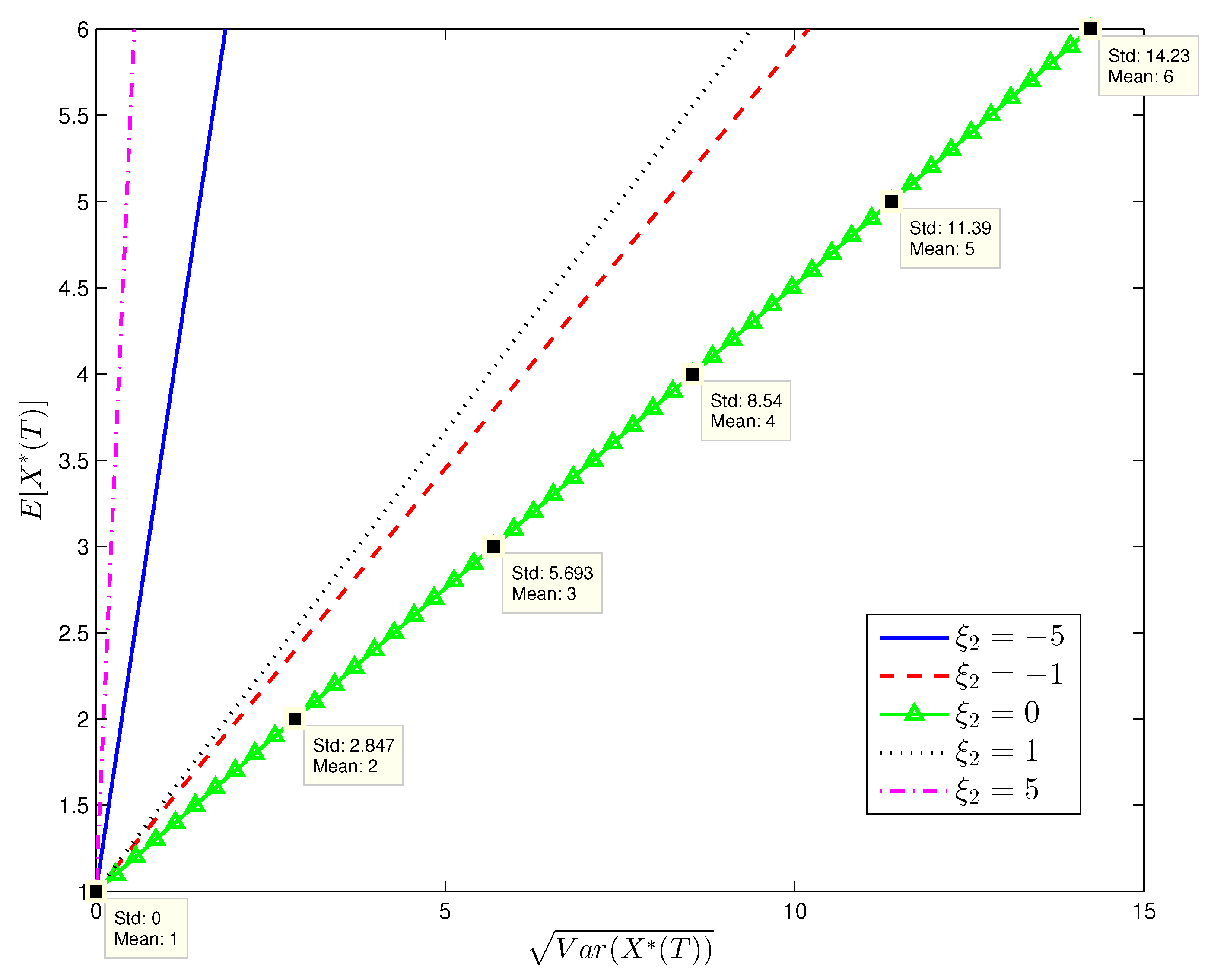
Figure 1, Figure 2, Figure 3 and Figure 4 show the efficient frontiers (standard deviation v.s. mean) with different values of ${\xi }_1$ and ${\xi }_2$. From Figure 1, Figure 2, Figure 3 and Figure 4, the efficient frontiers in the complete market is always on the left hand side of those in the incomplete market when all parameter values are identical. Note that the efficient frontier on the left hand side has a greater slope and a greater slope indicates a lower overall portfolio risk. This shows that introducing the variance swap to the financial market is an effective way to hedge the volatility risk, thereby reducing the overall risk of the agent’s terminal wealth. From Figure 1 and Figure 2, we can see that the overall risk of the agent’s terminal wealth decreases with ${\xi }_1$. On the one hand, observing two matrices in Equation (83) and using the comparison theorem for Riccati equations, we know that both $h(0)$ and $g(0)$ are increasing functions of ${\xi }_1$ when the values of other model parameters are specified in Table 1. In addition, the greater is $h(0)$ or $g(0)$, the greater is the slope in (47) or (82). Thus, the efficient frontiers with greater ${\xi }_1$ are on the left hand side of those with smaller ${\xi }_1$. If the market price of the common risk ${\xi }_1$ is higher, the excessive returns on both the stock and the variance are greater. Therefore, the agent can achieve a same level of expected terminal wealth by holding less risky assets and hence bearing less risk.

In Figure 4, it is shown that ${\xi }_2$ has no impact on the efficient frontiers in the incomplete market. In the incomplete market, the agent cannot invest in the variance swap and does not bear the idiosyncratic risk of the variance process in his wealth. So the efficient frontiers in the incomplete market are independent of ${\xi }_2$. On the other hand, Figure 3 shows that the efficient frontiers in the complete market with the variance swap do vary with ${\xi }_2$. Regardless of whether ${\xi }_2$ is negative or positive, the variance of the terminal wealth in the complete market is smaller than that in the incomplete market for any given level of expected terminal wealth. Moreover, the higher is the absolute value of ${\xi }_2$, the smaller variance of the terminal wealth can be achieved in the complete market. Note that ${\xi }_2$ is proportional to the market price of the idiosyncratic risk of the variance process. This implies that the higher is the market price of the idiosyncratic risk, the more volatility risk can be hedged by the variance swap. We note that even if ${\xi }_2$ is zero, the variance is also slightly smaller in Figure 3 than in Figure 4 (refer to the green lines in both figures). This implies that even when the idiosyncratic risk is not priced, the volatility risk still amplifies the variance of the terminal wealth and the variance swap can be still used to hedge the volatility risk in the complete market.

Table 2. The efficient frontier in the complete market with different $\rho$.

	$\mathbb{E}\left[{\mathit{X}}^{*}(\mathit{T})\right]$	1.0	2.0	3.0	4.0	5.0	6.0
Parameter Values		$\sqrt{\mathbf{Var}\left[{\mathit{X}}^{*}(\mathit{T})\right]}$
$\rho$	−1.0	0	2.916508	5.833017	8.749525	11.666033	14.582542
	−0.9	0	1.956137	3.912274	5.868411	7.824548	9.780685
	−0.8	0	1.930803	3.861606	5.792409	7.723212	9.654014
	−0.7	0	1.910073	3.820146	5.730219	7.640291	9.550364
	−0.6	0	1.891954	3.783907	5.675861	7.567814	9.459768
	−0.5	0	1.875674	3.751348	5.627022	7.502696	9.378370
	−0.4	0	1.860846	3.721692	5.582538	7.443384	9.304230
	−0.3	0	1.847249	3.694498	5.541748	7.388997	9.236246
	−0.2	0	1.834752	3.669504	5.504257	7.339009	9.173761
	−0.1	0	1.823279	3.646558	5.469836	7.293115	9.116394
	0.0	0	1.812791	3.625582	5.438374	7.251165	9.063956
	1.0	0	2.650105	5.300211	7.950316	10.600422	13.250527

and

Table 3. The efficient frontier in the incomplete market with different $\rho$.

	$\mathbb{E}\left[{\mathit{Y}}^{*}(\mathit{T})\right]$	1.0	2.0	3.0	4.0	5.0	6.0
Parameter Values		$\sqrt{\mathbf{Var}{[\mathit{Y}}^{*}(\mathit{T})]}$
$\rho$	−1.0	0	2.916508	5.833017	8.749525	11.666033	14.582542
	−0.9	0	2.902382	5.804764	8.707145	11.609527	14.511909
	−0.8	0	2.888341	5.776681	8.665022	11.553363	14.441704
	−0.7	0	2.874385	5.748770	8.623155	11.497540	14.371926
	−0.6	0	2.860515	5.721030	8.581545	11.442060	14.302575
	−0.5	0	2.846731	5.693461	8.540192	11.386922	14.233653
	−0.4	0	2.833031	5.666063	8.499094	11.332126	14.165157
	−0.3	0	2.819418	5.638835	8.458253	11.277671	14.097089
	−0.2	0	2.805889	5.611778	8.417668	11.223557	14.029446
	−0.1	0	2.792446	5.584892	8.377337	11.169783	13.962229
	0.0	0	2.779087	5.558174	8.337261	11.116349	13.895436
	1.0	0	2.650105	5.300211	7.950316	10.600422	13.250527

1 report the efficient frontiers with different $\rho$ in the complete and the incomplete markets, respectively. Though $\rho <0$ is a condition to incorporate the leverage effect in our modeling framework, we also show the efficient frontiers with $\rho =1$, as this case corresponds to a degenerate incomplete market, which is in fact complete as discussed throughout this paper. We observe that as the correlation increases from $-1$ to 0, the variance of the terminal wealth is decreasing in both markets. This is because that the increase of $\rho$ reduces the leverage effect, which makes the stock price risk and volatility risk less interactive. Thus, the diminished interaction decreases the overall risk of the terminal wealth.

It is particularly interesting, as shown in the first and the last rows of Table 2 and Table 3, that the efficient frontiers are exactly the same in the complete and the incomplete markets when $\rho =\pm 1$. This verifies our conjecture, that is, $\rho =\pm 1$ is a condition that the complete and the incomplete markets are indistinguishable. The equivalence of two markets can be also confirmed by the comparison theorem of Riccati equations. More precisely, the following equality holds

$$\begin{array}{c}\hfill \left(\begin{array}{cc}{\xi }_1^2& -(\kappa +2\sigma {\xi }_1\rho )\\ 0& ({\rho }^2-\frac{1}{2}){\sigma }^2\end{array}\right)=\left(\begin{array}{cc}{\xi }_1^2+{\mathbf{1}}_{\{{\rho }^2\ne \pm 1\}}{\xi }_2^2& -(\kappa +2\sigma {\xi }_{\rho })\\ 0& \frac{1}{2}{\sigma }^2\end{array}\right).\end{array}$$

(84)

if and only if $\rho =\pm 1$. Once Equation (84) is satisfied, the slopes in (47) and (82) are identical and so are the efficient frontiers. If the variance process and the stock price process are perfectly positive/negative-correlated (i.e., $\rho =\pm 1$), the variance swap becomes a redundant asset. Note that even if the idiosyncratic risk is not priced, i.e., ${\xi }_2=0$, the two matrices in (84) may be still different due to their last entries (see Figure 3 and Figure 4). This reflects that the differences of the complete market and the incomplete market are primarily determined by $\rho$ rather than ${\xi }_2$.

7. Conclusions

In this paper, we investigate the effect of the variance swap in hedging volatility risk by solving two mean-variance portfolio selection problems under Heston’s model. The LQ control and BSDE approach is used to tackle the problems. We obtain explicit expressions of the efficient portfolio strategies and the efficient frontiers in the complete and the incomplete markets. Numerical examples demonstrate that investing in the complete market with the variance swap can achieve a smaller variance (i.e., risk) of the terminal wealth than in the incomplete market without the variance swap.

The paper only considers a single-factor stochastic volatility model, namely Heston’s model. In future research, it is interesting to use more realistic stochastic volatility models, e.g., multivariate Heston model (refer to Asai et al. (2006)). Another potential direction is to include other variance/volatility derivatives into the investment portfolio, such as volatility swaps, VIX futures, and VIX options.

References

- Asai, Manabu, Michael McAleer, and Jun Yu. 2006. Multivariate stochastic volatility: A review. Econometric Reviews 25: 145–75. [Google Scholar] [CrossRef]
- Biagini, Francesca, Paolo Guasoni, and Maurizio Pratelli. 2000. Mean-Variance hedging for stochastic volatility models. Mathematical Finance 10: 109–23. [Google Scholar] [CrossRef] [Green Version]
- Black, Fisher, and Myron Scholes. 1973. The pricing of options and corporate liabilities. The Journal of Political Economy 81: 637–54. [Google Scholar] [CrossRef] [Green Version]
- Briand, Philippe, and Ying Hu. 2008. Quadratic BSDEs with convex generators and unbounded terminal conditions. Probability Theory and Related Fields 141: 543–67. [Google Scholar] [CrossRef] [Green Version]
- Černý, Aleš, and Jan Kallsen. 2008. Mean-variance hedging and optimal investment in Heston’s model with correlation. Mathematical Finance 18: 473–92. [Google Scholar]
- Chacko, George, and Luis M. Viceira. 2005. Dynamic consumption and portfolio choice with stochastic volatility in incomplete markets. The Review of Financial Studies 18: 1369–402. [Google Scholar] [CrossRef] [Green Version]
- Chiu, Mei Choi, and Hoi Ying Wong. 2011. Mean-variance portfolio selection of cointegrated assets. Journal of Economic Dynamics and Control 35: 1369–85. [Google Scholar] [CrossRef]
- Chiu, Mei Choi, and Hoi Ying Wong. 2014. Mean-variance portfolio selection with correlation risk. Journal of Computational and Applied Mathematics 263: 432–44. [Google Scholar] [CrossRef]
- Cohen, Samuel N., and Robert James Elliott. 2015. Stochastic Calculus and Applications, 2nd ed. Basel: Birkhäuser. [Google Scholar]
- Duffee, Gregory R. 2002. Term premia and interest rate forecasts in affine models. The Journal of Finance 57: 405–43. [Google Scholar] [CrossRef]
- Dupire, Bruno. 1992. Arbitrage Pricing with Stochastic Volatility. Paris: Options Division, Société Générale. [Google Scholar]
- Dupire, Bruno. 1993. Model art. Risk 6: 118–24. [Google Scholar]
- El Karoui, Nicole, Shige Peng, and Marie Claire Quenez. 1997. Backward stochastic differential equations in finance. Mathematical Finance 7: 1–71. [Google Scholar] [CrossRef]
- Elliott, Robert James, and P. Ekkehard Kopp. 2005. Mathematics of Financial Markets. New York: Springer. [Google Scholar]
- Fleming, Wendell H., and Daniel Hernández-Hernández. 2003. An optimal consumption model with stochastic volatility. Finance and Stochastics 7: 245–62. [Google Scholar] [CrossRef]
- Freiling, Gerhard, Gerhard Jank, and Hisham Abou-Kandil. 1996. Generalized Riccati difference and differential equations. Linear Algebra and its Applications 241: 291–303. [Google Scholar] [CrossRef] [Green Version]
- French, Kenneth R., G. William Schwert, and Robert F. Stambaugh. 1987. Expected stock returns and volatility. Journal of Financial Economics 19: 3–29. [Google Scholar] [CrossRef] [Green Version]
- Heston, Steven L. 1993. A closed-form solution for options with stochastic volatility with applications to bond and currency options. The Review of Financial Studies 6: 327–43. [Google Scholar] [CrossRef] [Green Version]
- Hobson, David. 2004. Stochastic volatility models, correlation, and the q-optimal measure. Mathematical Finance 14: 537–56. [Google Scholar] [CrossRef]
- Hull, John, and Alan White. 1987. The pricing of options on assets with stochastic volatilities. The Journal of Finance 42: 281–300. [Google Scholar] [CrossRef]
- Kallsen, Jan, and Johannes Muhle-Karbe. 2010. Utility maximization in affine stochastic volatility models. International Journal of Theoretical and Applied Finance 13: 459–77. [Google Scholar] [CrossRef] [Green Version]
- Kraft, Holger. 2005. Optimal portfolios and Heston’s stochastic volatility model: An explicit solution for power utility. Quantitative Finance 5: 303–13. [Google Scholar] [CrossRef]
- Kobylanski, Magdalena. 2000. Backward stochastic differential equations and partial differential equations with quadratic growth. Annals of Probability 28: 558–602. [Google Scholar] [CrossRef]
- Laurent, Jean Paul, and Huyên Pham. 1999. Dynamic programming and mean-variance hedging. Finance and Stochastics 3: 83–110. [Google Scholar] [CrossRef]
- Li, Danping, Yang Shen, and Yan Zeng. 2018. Dynamic derivative-based investment strategy for mean-variance asset-liability management with stochastic volatility. Insurance: Mathematics and Economics 78: 72–86. [Google Scholar] [CrossRef]
- Lim, Andrew E. B. 2004. Quadratic hedging and mean-variance portfolio selection with random parameters in an incomplete market. Mathematics of Operations Research 29: 132–61. [Google Scholar] [CrossRef] [Green Version]
- Lim, Andrew E. B. 2005. Mean-variance hedging when there are jumps. SIAM Journal on Control and Optimization 44: 1893–922. [Google Scholar] [CrossRef] [Green Version]
- Lim, Andrew E. B., and Xun Yu Zhou. 2002. Mean-variance portfolio selection with random parameters in a complete market. Mathematics of Operations Research 27: 101–20. [Google Scholar] [CrossRef] [Green Version]
- Liu, Jun, Francis A. Longstaff, and Jun Pan. 2003. Dynamic asset allocation with event risk. The Journal of Finance 58: 231–59. [Google Scholar] [CrossRef] [Green Version]
- Luenberger, David G. 1968. Optimization by Vector Space Methods. New York: John Wiley. [Google Scholar]
- Markowitz, Harry. 1952. Portfolio Selection. The Journal of Finance 7: 77–91. [Google Scholar]
- Merton, Robert C. 1969. Lifetime portfolio selection under uncertainty: The continuous-time case. The Review of Economics and Statistics 51: 247–57. [Google Scholar] [CrossRef] [Green Version]
- Merton, Robert C. 1971. Optimum consumption and portfolio rules in a continuous-time model. Journal of Economic Theory 3: 373–413. [Google Scholar] [CrossRef]
- Neuberger, Anthony J. 1990. Volatility Trading. London: Institute of Finance and Accounting, London Business School. [Google Scholar]
- Neuberger, Anthony J. 1994. The log contract. The Journal of Portfolio Management 20: 74–80. [Google Scholar] [CrossRef]
- Shen, Yang, and Yan Zeng. 2015. Optimal investment-reinsurance for mean-variance insurers with square-root factor process. Insurance: Mathematics and Economics 62: 118–37. [Google Scholar] [CrossRef]
- Shen, Yang, Xin Zhang, and Tak Kuen Siu. 2014. Mean-variance portfolio selection under a constant elasticity of variance model. Operations Research Letters 42: 337–42. [Google Scholar] [CrossRef]
- Shen, Yang. 2015. Mean-variance portfolio selection in a random environment with unbounded coefficients. Automatica 55: 165–75. [Google Scholar] [CrossRef]
- Stein, Elias M., and Jeremy C. Stein. 1991. Stock price distributions with stochastic volatility: An analytic approach. The Review of Financial Studies 4: 727–52. [Google Scholar] [CrossRef]
- Wiggins, James B. 1987. Option values under stochastic volatility: Theory and empirical estimates. Journal of Financial Economics 19: 351–72. [Google Scholar] [CrossRef]
- Yong, Jiongmin, and Xun Yu Zhou. 1999. Stochastic Controls: Hamiltonian Systems and HJB Equations. New York: Springer. [Google Scholar]
- Zariphopoulou, Thaleia. 2001. A solution approach to valuation with unhedgeable risks. Finanance and Stochastics 5: 61–82. [Google Scholar] [CrossRef]
- Zeng, Xudong, and Michael Taksar. 2013. A stochastic volatility model and optimal portfolio selection. Quantitative Finance 13: 1547–58. [Google Scholar] [CrossRef]
- Zhou, Xun Yu, and Duan Li. 2000. Continuous-time mean-variance portfolio selection: A stochastic LQ framework. Applied Mathematics and Optimization 42: 19–33. [Google Scholar] [CrossRef]