Comparison of Home Advantage in European Football Leagues

Abstract

Home advantage in sports is important for coaches, players, fans, and commentators and has a key role in sports prediction models. This paper builds on results of recent research that—instead of points gained—used goals scored and goals conceded to describe home advantage. This offers more detailed look at this phenomenon. Presented description understands a home advantage in leagues as a random variable that can be described by a trinomial distribution. The paper uses this description to offer new ways of home advantage comparison—based on the Jeffrey divergence and the test for homogeneity—in different leagues. Next, a heuristic procedure—based on distances between probability descriptions of home advantage in leagues—is developed for identification of leagues with similar home advantage. Publicly available data are used for demonstration of presented procedures in 19 European football leagues between the 2007/2008 and 2016/2017 seasons, and for individual teams of one league in one season. Overall, the highest home advantage rate was identified in the highest Greek football league, and the lowest was identified in the fourth level English football league.

1. Introduction

The effect of home advantage is important in modeling the probabilities of the results of sports matches. These probabilities are the basis for listing odds for sports matches and therefore it is important for betting companies to have a good model for their estimation. Since the probabilities of the results of sports matches are not known (unlike, for example, in roulette), bookmakers are exposed to the risk of loss. The risk can be reduced by increasing their margin, but this reduces the competitiveness of bookmakers. Recent study of margins in English football leagues can be found in (Marek 2018) and it shows that bookmakers have significantly reduced margins in recent years. Next, results of (Buhagiar et al. 2018) show “that bettors lose more on events that are more accurately predicted by bookmakers”. Therefore, it is important to cover all available aspects that can improve the bookmakers’ models. This article is focused on one important factor—home advantage.

Home advantage in sports is addressed by many researchers. The main causes of the home advantage—crowd effect, referee bias, travel effect, familiarity with local conditions, territoriality, special tactics, etc.—are analysed and discussed in detail by (Pollard and Gómez 2014), and the scientific interest in this area can be tracked back to (Schwartz and Barsky 1977). Exhaustive studies about home advantage can be found in (Allen and Jones 2014) and (Pollard and Pollard 2005). In both papers, as well as in many others, the home advantage of a league is based on comparing the number of points that were earned at home grounds with the total number of points that were awarded. This approach, proposed by (Pollard 1986), is straightforward, easy to use, and produces reasonable results for a league as a whole. Adjustment that is required when the approach is used for individual teams is described in (Pollard and Ruano 2009); nevertheless, this procedure requires data over several seasons.

All papers mentioned in the previous paragraph understand home advantage similarly as defined in (Pollard and Pollard 2005): “the number of points obtained by the home team expressed as a percentage of all points obtained in all games played”. However, this definition can be problematic in some situations, e.g., let us assume that two teams A and B played each other exactly two times in a season. Team A recorded 4–0 win at its home ground and 2–0 win away from home. When points are used in this situation we conclude that the team A won exactly half of its points at its home ground. This leads to a conclusion that the team A does not have home advantage. However, using the difference of goals scored and conceded—for the team A: four goals at its home ground and two goals away from home—indicates that the team A recorded better result (measured only by the goal difference) at the home ground, i.e., it has the home advantage. The team B lost by two goals at its home ground and by four goals away from home. As in the case of the team A, the result at its home ground was better. If the similar situation happens often in a league then analysis may end with a conclusion that the home advantage—understood in its natural meaning—does not exist, or the home advantage can be underestimated.

The solution of this problem can be in using goals instead of points. This provides a deeper view of the home advantage problem, and it is closer to the natural meaning of the home advantage, i.e., better performance, not only more points. There are several approaches how to deal with goals, the first approach—based on modelling team ability and home advantage—was used by (Clarke and Norman 1995) for the analysis of home advantage of individual clubs in English football leagues. These models can be tracked back to (Maher 1982) and are usually used to predict match outcomes in football and other sports, e.g., (Karlis and Ntzoufras 2003) in water polo, (Marek et al. 2014) in ice hockey. Next approach is presented by (Goumas 2017) who models home advantage for individual teams in UEFA Championship League. His method is based on ratio of goals that was scored by the team at its home ground and total number of goals scored at its home ground, i.e., goals that the home team scored and conceded at its home ground. The third approach, on which this paper builds, was proposed by (Marek and Vávra 2017), and it uses a combined measure of home advantage that takes into account results (goals scored and conceded) of two same teams in one season, once at the home ground and once at the away team ground. The number of goals scored and conceded was successfully used in another type of analysis, e.g., (Hassanniakalager and Newall 2019) who analysed the potential variation in soccer betting outcomes—they used the cumulative number of points earned and the number of goals scored and conceded over the previous five matches.

The approach presented in this paper allows evaluation of home advantage for a single team in one season. It can also be used to evaluate home advantage of larger groups of data: league in one season, league over several seasons, and one team over several seasons. The price for this advantage is that only leagues with a balanced schedule can be analysed; nevertheless, this is the most common type of schedule in association football, and all leagues analysed in this paper use it.

The following parts present definition of home advantage based on goals scored and conceded. It uses three-state random variable that describes home advantage of a given object of interest: a team in a single season, a team over several seasons, a league in one season, and a league over several seasons. The main goals of this paper are to offer a usable procedure based on goals scored and conceded for evaluation of home advantage and procedure for identification of objects—leagues or teams—with similar type of home advantage. Leagues from the following countries are analysed in this paper: Belgium, the Czech Republic, England, France, Germany, Greece, Italy, Netherlands, Portugal, Spain, and Turkey (for some countries, even the lower level leagues are used). The 2015/2016 season of the top-level leagues of similar countries was analysed using method based on points in (Leite 2017), and it can be used for comparison of results.

2. Data

Leagues used in this paper are:

• Belgium: Belgian First Division A (level 1, $B{E}_1$);
• Czech Republic: Czech First League (level 1, $C{Z}_1$);
• England: Premier League (level 1, $E{N}_1$), English Football League Championship (level 2, $E{N}_2$), English Football League One (level 3, $E{N}_3$), English Football League Two (level 4, $E{N}_4$), and National League (level 5, $E{N}_5$);
• France: Ligue 1 (level 1, $F{R}_1$) and Ligue 2 (level 2, $F{R}_2$);
• Germany: Bundesliga (level 1, $D{E}_1$) and 2. Bundesliga (level 2, $D{E}_2$);
• Greece: Superleague Greece (level 1, $G{R}_1$);
• Italy: Serie A (level 1, $I{T}_1$) and Serie B (level 2, $I{T}_2$);
• Netherlands: Eredivisie (level 1, $N{L}_1$);
• Portugal: Primeira Liga (level 1, $P{T}_1$);
• Spain: La Liga (level 1, $E{S}_1$) and Segunda Divisíon (level 2, $E{S}_2$);
• Turkey: Süper Lig (level 1, $T{R}_1$).

All results starting 2007/2008 season and ending 2016/2017 season are used in the analysis. These results were obtained from (Football-Data.co.uk 2018) and (HETliga.cz 2018). Official websites of leagues e.g., LaLiga.es (2018) were used for basic data check, and to identify awarded wins1 which, obviously, do not represent abilities of teams. The whole of the 2014/2015 season of $G{R}_1$ was excluded from the analysis because of too many awarded wins. Awarded wins were also recorded in the following matches: Trabzonspor vs. Sivasspor (2007/2008, $T{R}_1$), Belenenses vs. Naval (2007/2008, $P{T}_1$), Bohemians 1905 vs. Bohemians Praha (2009/2010, $C{Z}_1$), Gaziantepspor vs. Bursaspor (2010/2011, $T{R}_1$), Bursaspor vs. Besiktas (2010/2011, $T{R}_1$), Aris vs. Tripolis (2011/2012, $G{R}_1$), Panathinaikos vs. Olympiakos (2011/2012, $G{R}_1$), AEK vs. Panthrakikos (2012/2013, $G{R}_1$), Besiktas vs. Galatasaray (2013/2014, $T{R}_1$), Trabzonspor vs. Fenerbahce (2013/2014, $T{R}_1$), Blackpool vs. Huddersfield (2014/2015, $E{N}_2$), Panathinaikos vs. Olympiakos (2015/2016, $G{R}_1$), Bastia vs. Lyon (2016/2017, $F{R}_1$), and Sassuolo vs. Pescara (2016/2017, $I{T}_1$). These matches were excluded from the analysis. Opposite matches between mentioned teams were also excluded as the analysis requires to have both matches played. The rest of the 72,182 matches were used in the analysis.

3. Methods

Three types of measures are defined in (Marek and Vávra 2017): active measure of home advantage (it uses difference between goals scored at home and away from home); passive measure of home advantage (it uses difference between goals conceded at home and away from home); and combined measure of home advantage (it uses both goals scored and conceded) which is used in this paper and described in Definition 1.

Definition 1.

Combined measure of home advantage is random variable C that can take values $-1,0$, and 1. $C=-1$ for team $T_1$ if two matches between teams $T_1$ and $T_2$ in a season ended with a better result – measured by goal differences in matches – for team $T_1$ away from home (at $T_2$’s ground). $C=0$ for team $T_1$ if goal differences in both matches were exactly the same from $T_1$’s point of view, and $C=1$ for team $T_1$ if this team recorded better result – measured by goal differences in matches – at its own ground. With results $h_{T_1}:a_{T_2}$ at the home ground of team $T_1$ and $h_{T_2}:a_{T_1}$ at the home ground of team $T_2$ the value of random variable C for team $T_1$ is determined as

$$C=sgn((h_{T_1}-a_{T_2})-(a_{T_1}-h_{T_2})).$$

(1)

3.1. Parameters Estimation Method

A balanced schedule was used in all leagues and seasons, i.e., each team played every other team exactly twice in a season, once at home and once away from home. The combined measure of home advantage combines results of the first half of the season (team A plays at its home ground against team B) with results of the second half of the season (team A plays against team B at B’s home ground). This means that 72,182 matches offers 36,091 observations of combined measure of home advantage.

Let $Z_r,r=-1,0,1$ are random variables which describe number of cases (e.g., for a team in a season) where it is possible to identify home advantage ($r=1$), away advantage ($r=-1$), and no advantage ($r=0$), i.e., $Z_r$ sums number of cases where $C=r$. Vector $(Z_{-1},Z_0,Z_1)$ follows trinomial distribution with parameters $p_{-1},p_0,p_1$, and K with probability function

$$P(k_{-1},k_0,k_1)=\frac{K!}{k_{-1}!k_0!k_1!}{p}_{-1}^{k_{-1}}{p}_0^{k_0}{p}_1^{k_1},$$

(2)

where K is total number of observations of combined measure in a season, $p_{-1},p_0,p_1$ are probabilities of occurring home advantage ($r=1$), away advantage ($r=-1$), and no advantage ($r=0$). $k_{-1},k_0,k_1$ ($k_{-1}+k_0+k_1=K$) are observations of appropriate advantage.

Maximum likelihood estimator of parameters $p_r,r=-1,0,1$ is

$${\widehat{p}}_r=\frac{k_r}{K},r=-1,0,1.$$

(3)

The procedure is demonstrated on results of $B{E}_1$ (Belgian First Division A) and $E{S}_1$ (La Liga) in the 2016/2017 season.

Table 1. Combined measure of home advantage in the 2016/2017 season—observed counts.

League	${\mathit{k}}_{-1}$	${\mathit{k}}_0$	${\mathit{k}}_1$
$B{E}_1$	33	13	74
$E{S}_1$	52	41	97

contains observed counts for combined measure and

Table 2. Estimated probabilities in the 2016/2017 season.

League	${\widehat{\mathit{p}}}_{-1}$	${\widehat{\mathit{p}}}_0$	${\widehat{\mathit{p}}}_1$
$B{E}_1$	0.275	0.108	0.617
$E{S}_1$	0.274	0.216	0.511

contains point estimates of parameters $p_r,r=-1,0,1$.

3.2. Comparison Methods

Home advantages of leagues were compared by two approaches. The first approach is based on Jeffrey divergence ($JD$), i.e., symmetric version of Kullback–Leibler distance. Jeffrey divergence (described in detail in (Deza and Deza 2006, p. 185)) can be used to measure distance between two probability distributions P and Q as

$$JD(P,Q)=\sum _x\left(p\left(x\right)ln\frac{p\left(x\right)}{q\left(x\right)}+q\left(x\right)ln\frac{q\left(x\right)}{p\left(x\right)}\right).$$

(4)

Equation (4) is used to measure distance between probability distributions of $(Z_{-1},Z_0,Z_1)$ for each two leagues or teams. Obtained distances are compared to find leagues or teams with home advantage that is similar (or different). Values of $JD$ are multiplied by 100 for better readability. For the data presented in Table 2 we obtain 100·JD = 9.410.

The second approach is based on the test for homogeneity of parallel samples that allows to test hypothesis $H_0$: two samples come from the same population (or in this case: that home advantage in both tested leagues, or for both tested teams, is described by the same distribution) against alternative hypothesis $H_1$: two samples do not come from the same population (or in this case: that home advantage in both tested leagues, or for both tested teams, is described by different distributions). ${\chi }^2$ statistic can be computed for a case with two leagues or two teams as

$${\chi }^2=\sum _{r=-1}^1\frac{{\left(k_{1,r}-\frac{k_{1,•}{k}_{•,r}}{k_{•,•}}\right)}^2}{\frac{k_{1,•}{k}_{•,r}}{k_{•,•}}}+\sum _{r=-1}^1\frac{{\left(k_{2,r}-\frac{k_{2,•}{k}_{•,r}}{k_{•,•}}\right)}^2}{\frac{k_{2,•}{k}_{•,r}}{k_{•,•}}},$$

(5)

where appropriate observed numbers ($k_{1,-1},k_{1,0},$ etc.) are obtained according to

Table 3. Observed numbers in given sample and class.

	$\mathit{C}=-1$	$\mathit{C}=0$	$\mathit{C}=1$	Total
Sample 1	$k_{1,-1}$	$k_{1,0}$	$k_{1,1}$	$k_{1,•}$
Sample 2	$k_{2,-1}$	$k_{2,0}$	$k_{2,1}$	$k_{2,•}$
Total	$k_{•,-1}$	$k_{•,0}$	$k_{•,1}$	$k_{•,•}$

.

Asymptotical distribution of ${\chi }^2$ statistic for the data in Table 3 is ${\chi }^2$ distribution with two degrees of freedom. For more details on this test see (Rao 2002, pp. 398–402).

Value of ${\chi }^2$ for the data in Table 1 is 6.378, and corresponding p-value is 0.094. The hypothesis $H_0$ that home advantage in $B{E}_1$ (Belgian First Division A) and $E{S}_1$ (La Liga) in the 2016/2017 season is described by the same distribution cannot be rejected, i.e., the null hypothesis that there is no difference in the home advantage (measured by the combined measure) in $B{E}_1$ and $E{S}_1$ in the 2016/2017 season cannot be rejected.

The method based on ${\chi }^2$ statistic can be used to test whether the home advantage in two leagues, or of two teams, differ or not. Next, both presented methods may be used as a heuristic procedure to identify groups of leagues, or teams, with similar home advantage. The steps of the procedure are:

(1)

Construct a graph, where leagues are used as vertices and distances (measured by $JD$ or ${\chi }^2$) are used as edges;

(2)

Find the edge with the highest distance and remove it from the graph;

(3)

Repeat step $\left(2\right)$ until the graph becomes disconnected, i.e., until two components are obtained.

This heuristic procedure will determine two groups (components) of leagues, or teams, where distance ($JD$ or ${\chi }^2$) between any league, or team, from the first group (component) and the second group (component) is always equal or greater than the last removed distance of the graph. The described procedure can continue to obtain more components.

4. Results

The first subsection will present the results obtained if only categorization by leagues is used, i.e., for each analysed league over whole 10 seasons. The second subsection will present major findings for single seasons, and the last subsection will demonstrate usage of this approach for single teams.

4.1. Categorization by Leagues

All findings in this chapter are valid for leagues over the last 10 seasons together (observed counts of combined measure in each season are connected together for each league to obtain one group of data for a league).

Observed counts of combined measure for each analysed league over all 10 seasons (from the 2007/2008 season to the 2016/2017 season) are presented in

Table 4. Observed counts of combined measure for each analysed league over all 10 seasons with appropriate estimated probabilities.

League	Counts of Combined Measure				Estimated Probabilities
	$\mathit{k}=-1$	$\mathit{k}=0$	$\mathit{k}=1$	Total	${\widehat{\mathit{p}}}_{-1}$	${\widehat{\mathit{p}}}_0$	${\widehat{\mathit{p}}}_1$
$E{N}_1$	520	346	1034	1900	0.274	0.182	0.544
$E{N}_2$	796	510	1453	2759	0.289	0.185	0.527
$E{N}_3$	845	503	1412	2760	0.306	0.182	0.512
$E{N}_4$	922	518	1320	2760	0.334	0.188	0.478
$E{N}_5$	845	494	1398	2737	0.309	0.180	0.511
$D{E}_1$	461	234	835	1530	0.301	0.153	0.546
$D{E}_2$	461	243	826	1530	0.301	0.159	0.540
$E{S}_1$	484	304	1112	1900	0.255	0.160	0.585
$E{S}_2$	600	438	1272	2310	0.260	0.190	0.551
$I{T}_1$	502	344	1053	1899	0.264	0.181	0.555
$I{T}_2$	617	453	1240	2310	0.267	0.196	0.537
$F{R}_1$	507	341	1051	1899	0.267	0.180	0.553
$F{R}_2$	480	369	1051	1900	0.253	0.194	0.553
$N{L}_1$	422	247	861	1530	0.276	0.161	0.563
$B{E}_1$	329	236	686	1251	0.263	0.189	0.548
$P{T}_1$	364	243	691	1298	0.280	0.187	0.532
$T{R}_1$	416	289	803	1508	0.276	0.192	0.532
$G{R}_1$	287	221	753	1261	0.228	0.175	0.597
$C{Z}_1$	304	184	711	1199	0.254	0.153	0.593

.

The highest and lowest value of each column of estimated probabilities are highlighted. Test of hypothesis that home advantage exists can be tested by the procedure described in (Marek and Vávra 2017). The result of this test is that the null hypothesis about non-existent home advantage can be rejected, and the alternative hypothesis that home advantage exists can be accepted for all leagues in Table 4. The main goal of this paper is to build on these expected results, and to compare home advantage of leagues.

Each two leagues can be compared using the test for homogeneity of parallel samples described in Section 3.2. All p-values for each pair of the highest leagues of each country are listed in

Table 5. p-values of the test for homogeneity of parallel samples for the highest leagues over all ten seasons.

	${\mathit{EN}}_1$	${\mathit{DE}}_1$	${\mathit{ES}}_1$	${\mathit{IT}}_1$	${\mathit{FR}}_1$	${\mathit{NL}}_1$	${\mathit{BE}}_1$	${\mathit{PT}}_1$	${\mathit{TR}}_1$	${\mathit{GR}}_1$	${\mathit{CZ}}_1$
$E{N}_1$	−	0.038	0.033	0.781	0.844	0.268	0.771	0.804	0.726	0.006	0.021
$D{E}_1$	0.038	−	0.010	0.016	0.027	0.290	0.013	0.046	0.014	<0.001	0.017
$E{S}_1$	0.033	0.010	−	0.111	0.112	0.336	0.060	0.011	0.005	0.171	0.870
$I{T}_1$	0.781	0.016	0.111	−	0.980	0.297	0.866	0.453	0.436	0.036	0.062
$F{R}_1$	0.844	0.027	0.112	0.980	−	0.368	0.810	0.500	0.453	0.026	0.064
$N{L}_1$	0.268	0.290	0.336	0.297	0.368	−	0.165	0.140	0.074	0.014	0.274
$B{E}_1$	0.771	0.013	0.060	0.866	0.810	0.165	−	0.600	0.680	0.040	0.034
$P{T}_1$	0.804	0.046	0.011	0.453	0.500	0.140	0.600	−	0.940	0.002	0.007
$T{R}_1$	0.726	0.014	0.005	0.436	0.453	0.074	0.680	0.940	−	0.002	0.004
$G{R}_1$	0.006	<0.001	0.171	0.036	0.026	0.014	0.040	0.002	0.002	−	0.173
$C{Z}_1$	0.021	0.017	0.870	0.062	0.064	0.274	0.034	0.007	0.004	0.173	−

. In the case of $D{E}_1$, the hypothesis that home advantage is described by the same distribution cannot be rejected only in the case of testing with $N{L}_1$. Nevertheless, if all 19 leagues are taken into account, then the only league where tests against any other league result in conclusion that null hypothesis can be rejected, and the alternative that home advantage in both tested leagues is described by different distributions, is $E{N}_4$.

(Leite and Pollard 2018) compared differences in home advantage between level 1 and level 2 football leagues. They used data between the 2010/2011 season and the 2016/2017 season, i.e., similar data as used in this paper. Their analysis used method based on points gained, and they found out that in England, Germany, Spain, Italy, and France no difference in home advantage was recorded. To compare results, we performed the analysis for the same seasons. Obtained results are the same with one exception—Spain. In Spain, according to our analysis, the home advantage is different in both leagues with interpretation that in $E{S}_1$ the home advantage is higher. This indicates, that method based on combined measure can offer more detailed view of home advantage, and it is able to find differences that cannot be identified by some methods based on points.

The second approach of comparing is not based on testing but on measuring distance between distributions that describe home advantage. Jeffrey divergence (multiplied by 100) measures distances between each pair of leagues, and selected results are shown in

Table 6. Jeffrey divergence (multiplied by 100) for the highest leagues over all ten seasons.

	${\mathit{EN}}_1$	${\mathit{DE}}_1$	${\mathit{ES}}_1$	${\mathit{IT}}_1$	${\mathit{FR}}_1$	${\mathit{NL}}_1$	${\mathit{BE}}_1$	${\mathit{PT}}_1$	${\mathit{TR}}_1$	${\mathit{GR}}_1$	${\mathit{CZ}}_1$
$E{N}_1$	−	0.78	0.72	0.05	0.04	0.31	0.07	0.06	0.08	1.37	1.06
$D{E}_1$	0.78	−	1.09	0.97	0.85	0.32	1.27	0.88	1.13	2.83	1.22
$E{S}_1$	0.72	1.09	−	0.46	0.46	0.26	0.74	1.18	1.24	0.47	0.04
$I{T}_1$	0.05	0.97	0.46	−	0.00	0.29	0.04	0.21	0.20	0.89	0.76
$F{R}_1$	0.04	0.85	0.46	0.00	−	0.24	0.06	0.18	0.19	0.97	0.75
$N{L}_1$	0.31	0.32	0.26	0.29	0.24	−	0.52	0.56	0.69	1.24	0.39
$B{E}_1$	0.07	1.27	0.74	0.04	0.06	0.52	−	0.16	0.11	1.03	1.11
$P{T}_1$	0.06	0.88	1.18	0.21	0.18	0.56	0.16	−	0.02	1.93	1.60
$T{R}_1$	0.08	1.13	1.24	0.20	0.19	0.69	0.11	0.02	−	1.82	1.69
$G{R}_1$	1.37	2.83	0.47	0.89	0.97	1.24	1.03	1.93	1.82	−	0.57
$C{Z}_1$	1.06	1.22	0.04	0.76	0.75	0.39	1.11	1.60	1.69	0.57	−

. The highest value among all analysed leagues is recorded for $E{N}_4$ and $G{R}_1$ where $100·JD(E{N}_4,G{R}_1)=6.810$, and the lowest value is recorder for $E{N}_3$ and $E{N}_5$ where $100·JD(E{N}_3,E{N}_5)=0.004$.

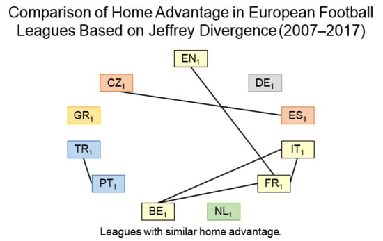
The procedure described in Section 3.2 is used to identify groups of leagues with similar home advantage, i.e., a graph where vertices represent leagues, and edges represent distances between leagues is constructed; edges with the highest distances are removed until a disconnected graph is obtained. The last removed edge is between $G{R}_1$ and $E{S}_1$ ($100·JD(G{R}_1,E{N}_1)=0.469$). After this, the graph contains two components, one with $G{R}_1$ and the second one with the remaining 18 leagues. As can be seen from Table 4, $G{R}_1$ shows a stronger home advantage than all the other leagues (parameter ${\widehat{p}}_1$). When the removing continues, the third component containing $E{N}_4$ is obtained; as can be seen from Table 4, $E{N}_4$ has the lowest home advantage. This procedure can continue further. Summary of all consequently obtained components is

• $G{R}_1$;
• $E{N}_4$;
• $D{E}_1$ and $D{E}_2$;
• $E{S}_1$ and $C{Z}_1$;
• $N{L}_1$;
• $E{N}_3$ and $E{N}_5$;
• $E{N}_2$, $I{T}_2$, $P{T}_1$, and $T{R}_1$.

The other six leagues $E{N}_1$, $E{S}_2$, $I{T}_1$, $F{R}_1$, $F{R}_2$, and $B{E}_1$ are in the largest component. The next removed distance would divide previously obtained components. Leagues in each group can be considered as those that poses similar home advantage.

The procedure based on ${\chi }^2$ statistics offers exactly the same results. The only difference is sequence of obtained components (e.g., the first obtained component is $E{N}_4$). In the case of ${\chi }^2$ statistics, the removed distance can be also connected with appropriate p-value from the test for homogeneity of parallel samples. As stated before, the first component contains $E{N}_4$, and it is obtained when the edge between $E{N}_4$ and $E{N}_5$ is removed. The value of ${\chi }^2$ statistics is 6.674 and corresponding p-value is 0.048 (i.e., the difference is still statistically significant at the 0.05 level of significance). The next component is obtained when edge between $G{R}_1$ and $C{Z}_1$ is removed. Corresponding p-value of this edge is 0.173. This means that the difference in home advantage for these two leagues cannot be considered as statistically significant at the 0.05 level of significance. However, as stated before, it is possible to use this approach as a heuristic procedure for identification of leagues with similar home advantage.

4.2. Categorization by Leagues and Seasons

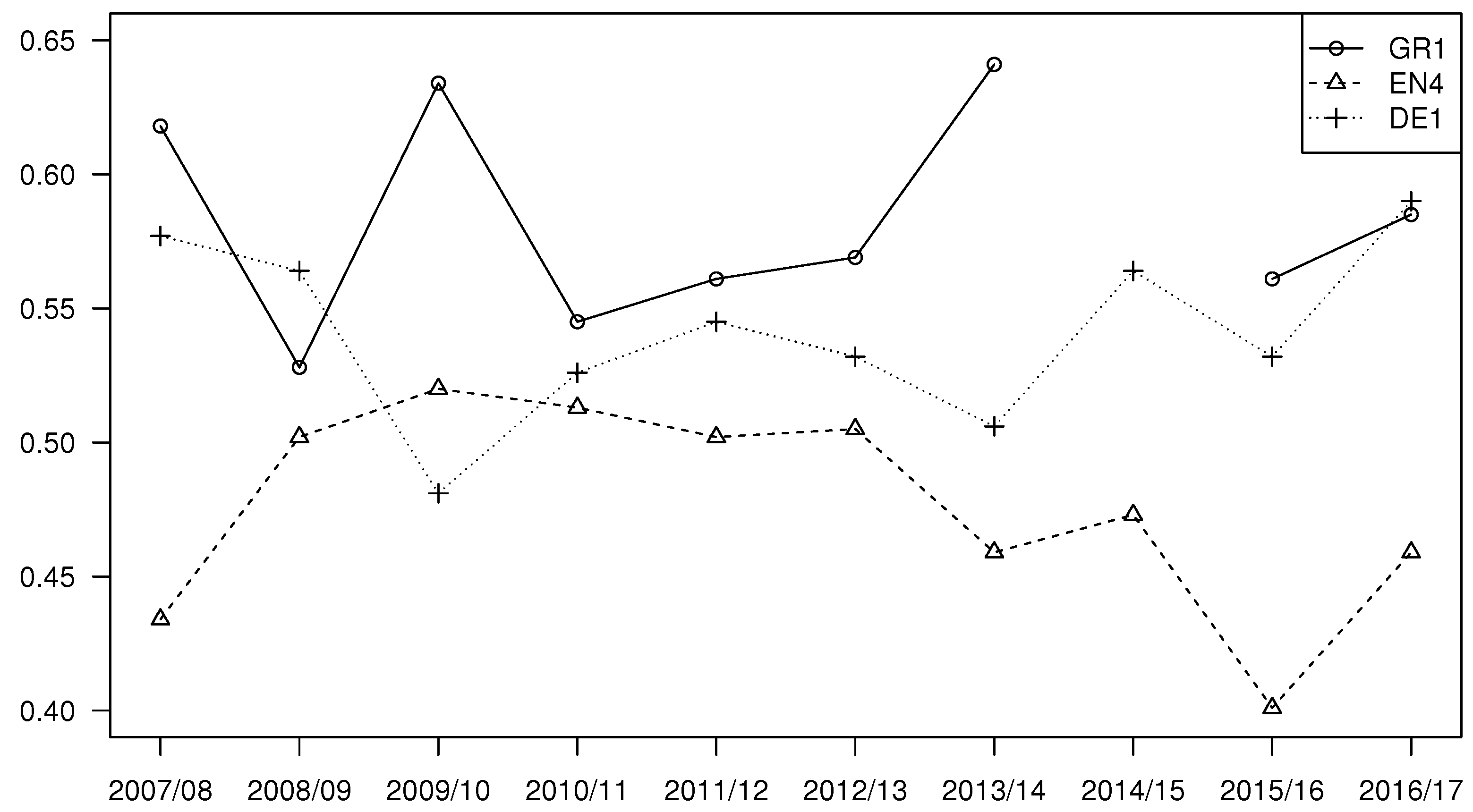
In the previous subsection, the highest difference in home advantage was identified between $E{N}_4$ and $G{R}_1$ (e.g., see Table 4); therefore, $E{N}_4$ and $G{R}_1$ are selected to present evolution of ${\widehat{p}}_1$ during all 10 seasons in Figure 1. The next league chosen for the presentation of results is $D{E}_1$ that recorded the lowest value of ${\widehat{p}}_0$ (see Table 4).

Point estimates ${\widehat{p}}_1$ of $G{R}_1$ are in all seasons (with an exception of 2015/2016 season that was excluded from the analysis; see Section 2) above the point estimates ${\widehat{p}}_1$ of $E{N}_4$ and usually above the point estimates ${\widehat{p}}_1$ of $D{E}_1$. The test for homogeneity of parallel samples described in Section 3.2 can be used to identify differences in home advantage between leagues in single seasons.

As an example, the test is used for each pair of leagues presented in Figure 1:

• The hypothesis $H_0$ that home advantage in $G{R}_1$ and $E{N}_4$ is described by the same distribution cannot be rejected in five seasons: 2008/2009, 2009/2010, 2010/2011, 2011/2012, and 2012/2013. The hypothesis $H_0$ can be rejected, and the alternative hypothesis $H_1$ that home advantage in $G{R}_1$ and $E{N}_4$ is described by different distributions can be accepted in four seasons: 2007/2008, 2013/2014, 2015/2016, and 2016/2017.
• The same test used for $G{R}_1$ and $D{E}_1$ shows that $H_0$ can be rejected, and $H_1$ can be accepted in three seasons: 2009/2010, 2010/2011, and 2013/2014 (the main difference in the 2010/2011 season is in values of ${\widehat{p}}_{-1}$ and ${\widehat{p}}_0$). $H_0$ cannot be rejected in the rest six seasons.
• The third tested pair is $D{E}_1$ and $E{N}_4$ for which $H_0$ can be rejected, and $H_1$ can be accepted in three seasons: 2007/2008, 2015/2016, and 2016/2017. $H_0$ cannot be rejected in the rest of the seven seasons.

Previous results suggest that when using data for a single season, the difference in home advantage between leagues must be substantial, otherwise it will not be identified. Therefore, to identify groups of leagues with similar home advantages, the heuristic procedure described in Section 3.2 will be used.

Table 7. Obtained components in seasons (based on ${\chi }^2$ distances).

Season	Lower Home Advantage	Higher Home Advantage
2007/2008	$E{N}_{4,5}$	all others
2008/2009	all others	$C{Z}_1$
2009/2010 *	$B{E}_1$
2010/2011	$E{N}_4,D{E}_1$	all others
2011/2012	all others	$B{E}_1$
2012/2013	$E{N}_{4,5},D{E}_{1,2}$	all others
2013/2014	$D{E}_2$	all others
2014/2015	$E{N}_3$	all others
2015/2016	$E{N}_4$	all others
2016/2017	all others	$B{E}_1$

contains, for each season analysed, the first two components identified by this procedure (distance was measured by ${\chi }^2$ statistic, see Equation (5)), e.g., the first of two obtained components in the 2007/2008 season contains $E{N}_4$ and $E{N}_5$, and the second component contains all other leagues. The interpretation of these results is based on values of ${\widehat{p}}_r,r=-1,0,1$—the first component includes leagues for which the ${\widehat{p}}_{-1}$ values are higher than for the leagues forming the second component.

Table 7 contains one remark (${}^{*}$) for the 2009/2010 season. The interpretation in this season is not made in favour of the higher or lower home advantage, because the different value (0.29) is obtained for ${\widehat{p}}_0$ which is the highest value for all leagues not only in this season but also in all tested seasons.

The 2015/2016 season of $B{E}_1$, $E{N}_1$, $F{R}_1$, $D{E}_1$, $I{T}_1$, $N{L}_1$, $P{T}_1$, $E{S}_1$, $T{R}_1$, and Russia was analysed in (Leite 2017) with the result that home advantage can be found in each of these leagues. Except for Russia, this paper contains all leagues that were analysed in (Leite 2017). The same approach as in (Leite 2017) was used to compute home advantage based on points for all 19 leagues used in this paper. Except for $E{N}_4$, all leagues can be considered to have home advantage based on points. When the combined measure that uses goals scored and conceded is used, and home advantage is tested by the procedure described in (Marek and Vávra 2017), then the result is the same, i.e., the null hypothesis about non-existent home advantage cannot be rejected only for $E{N}_4$.

Nevertheless, the interpretation of results based on obtained values is different, e.g., three teams with the highest home advantage based on points are $C{Z}_1$, $I{T}_2$, and $E{S}_2$. The approach presented in this paper provides more detailed view of home advantage (based on combined measure)—it offers the same interpretation for $C{Z}_1$ and $I{T}_2$, however in the case of $E{S}_2$ the home advantage is below average of all 19 leagues, and high value is obtained for the parameter ${\widehat{p}}_0$ (no advantage), i.e., the same difference at home and away.

This illustrates that both methods will probably answer the question about existence of home advantage in the similar way. The main difference is in the interpretation how strong is the home advantage and in the possibility of better understanding of home advantage.

Complete results for point estimate ${\widehat{p}}_1$ are contained in

Table 8. Results of ${\widehat{p}}_1$ for leagues in single seasons.

	07/08	08/09	09/10	10/11	11/12	12/13	13/14	14/15	15/16	16/17
$E{N}_1$	0.570	0.503	0.622	0.575	0.560	0.503	0.544	0.539	0.472	0.523
$E{N}_2$	0.534	0.559	0.584	0.523	0.509	0.513	0.477	0.496	0.509	0.541
$E{N}_3$	0.534	0.487	0.602	0.509	0.513	0.455	0.473	0.444	0.563	0.516
$E{N}_4$	0.434	0.502	0.520	0.513	0.502	0.505	0.459	0.473	0.401	0.459
$E{N}_5$	0.491	0.520	0.547	0.520	0.513	0.470	0.588	0.487	0.484	0.473
$D{E}_1$	0.577	0.564	0.481	0.526	0.545	0.532	0.506	0.564	0.532	0.590
$D{E}_2$	0.603	0.564	0.590	0.545	0.519	0.506	0.487	0.519	0.481	0.545
$E{S}_1$	0.570	0.523	0.601	0.622	0.617	0.622	0.575	0.591	0.585	0.508
$E{S}_2$	0.517	0.551	0.560	0.594	0.530	0.573	0.534	0.530	0.538	0.551
$I{T}_1$	0.534	0.580	0.575	0.560	0.560	0.549	0.528	0.508	0.570	0.544
$I{T}_2$	0.590	0.556	0.543	0.560	0.474	0.500	0.466	0.543	0.568	0.543
$F{R}_1$	0.580	0.539	0.523	0.580	0.565	0.508	0.544	0.544	0.544	0.570
$F{R}_2$	0.565	0.606	0.560	0.596	0.544	0.523	0.570	0.528	0.497	0.508
$N{L}_1$	0.583	0.564	0.596	0.571	0.564	0.532	0.577	0.513	0.526	0.558
$B{E}_1$	0.532	0.526	0.463	0.593	0.667	0.463	0.504	0.512	0.561	0.610
$P{T}_1$	0.537	0.520	0.512	0.480	0.561	0.472	0.528	0.551	0.532	0.571
$T{R}_1$	0.538	0.526	0.532	0.455	0.583	0.513	0.603	0.449	0.551	0.519
$G{R}_1$	0.618	0.528	0.634	0.545	0.561	0.569	0.641	—	0.561	0.585
$C{Z}_1$	0.585	0.634	0.537	0.585	0.520	0.577	0.626	0.642	0.650	0.512

. The table uses a tint to emphasize the values—the darker the higher the value of the ${\widehat{p}}_1$. These results can be used to assess whether or not there are large differences over the years in a single league. As we have seen before in Figure 1, the results can change significantly over the time. Stable results can be seen in $I{T}_1,N{L}_1,$ and $E{S}_2$. Big variance can be seen in $B{E}_1,E{N}_3,$ and $T{R}_1$. This information can be used by bookmakers and gamblers to identify leagues where home advantage plays significant role each year.

4.3. Home Advantage for Single Teams

Out of all leagues, the most surprising results were obtained for $E{N}_4$; therefore, it is chosen for demonstration of proposed approach for single teams. Again, as for leagues, it can be used over several seasons or even for a single season. The lowest recorded home advantage for $E{N}_4$ was in the 2015/2016 season; therefore, because it can offer a detailed view of home advantage of teams in this season, it is chosen for the demonstration of usage for single teams in a single season. Results are presented in

Table 9. Observed counts of combined measure for the 2015/2016 season of $E{N}_4$.

Team	Counts of Combined Measure				Estimated Probabilities
	$\mathit{k}=-1$	$\mathit{k}=0$	$\mathit{k}=1$	Total	${\widehat{\mathit{p}}}_{-1}$	${\widehat{\mathit{p}}}_0$	${\widehat{\mathit{p}}}_1$
Accrington	9	5	9	23	0.391	0.217	0.391
AFC Wimbledon	12	3	8	23	0.522	0.130	0.348
Barnet	8	1	14	23	0.348	0.043	0.609
Bristol Rvs	7	6	10	23	0.304	0.261	0.435
Cambridge	8	4	11	23	0.348	0.174	0.478
Carlisle	7	6	10	23	0.304	0.261	0.435
Crawley Town	6	6	11	23	0.261	0.261	0.478
Dag and Red	11	5	7	23	0.478	0.217	0.304
Exeter	10	5	8	23	0.435	0.217	0.348
Hartlepool	5	7	11	23	0.217	0.304	0.478
Leyton Orient	9	5	9	23	0.391	0.217	0.391
Luton	15	1	7	23	0.652	0.043	0.304
Mansfield	8	7	8	23	0.348	0.304	0.348
Morecambe	9	7	7	23	0.391	0.304	0.304
Newport County	8	7	8	23	0.348	0.304	0.348
Northampton	7	6	10	23	0.304	0.261	0.435
Notts County	8	5	10	23	0.348	0.217	0.435
Oxford	10	6	7	23	0.435	0.261	0.304
Plymouth	9	5	9	23	0.391	0.217	0.391
Portsmouth	10	5	8	23	0.435	0.217	0.348
Stevenage	10	5	8	23	0.435	0.217	0.348
Wycombe	12	3	8	23	0.522	0.130	0.348
Yeovil	8	5	10	23	0.348	0.217	0.435
York	6	3	14	23	0.261	0.130	0.609

. Strong home advantage can be identified only for two teams—Barnet and York. Totally, ${\widehat{p}}_1>{\widehat{p}}_{-1}$ for 10 out of 24 teams, ${\widehat{p}}_1<{\widehat{p}}_{-1}$ for 9 out of 24 teams, and ${\widehat{p}}_1={\widehat{p}}_{-1}$ for 5 out of 24 teams. These results demonstrate that surprising results about home advantage in $E{N}_4$ in the 2015/2016 season is not caused by several teams but, on the contrary, it is common for almost all teams.

Each two teams can be compared using the test for homogeneity of parallel samples described in Section 3.2. The team with the highest number of cases where the null hypothesis that home advantage of both tested teams is described by the same distribution can be rejected, and the alternative that home advantage of both tested teams is described by different distributions can be accepted is Luton. For Luton, 9 out of 23 teams can be considered as those with statistically significant difference in home advantage. The next team with most differences is Barnet with four cases.

The heuristic procedure based on searching for components of graph (see Section 3.2) can be used to identify groups of teams with similar home advantages. When distances are based on Jeffrey divergence, then the first obtained component is Luton with interpretation that it has lower home advantage. Next obtained components are: Barnet (higher home advantage), York (higher home advantage), AFC Wimbledon and Wycombe (lower home advantage), Hartlepool (higher home advantage), etc.

5. Conclusions

This paper described procedures based on combined measure of home advantage that can be used to compare home advantage of different leagues. Combined measure of home advantage is based on both goals scored and conceded, and this is the reason why it can detect home advantage in a better way than the usual approach based on points gained. Section 3.2 introduced two methods that can be used to compare home advantage. The first method is based on classical hypothesis testing, and the second method uses distances between leagues and heuristic procedure that can be used to find leagues with similar home advantage.

Described procedures were used in 10 seasons in 19 football leagues, and obtained results were compared. Results for all seasons together were used in Section 4.1; the Superleague Greece ($G{R}_1$) was identified as a league with the highest home advantage, and the English Football League Two ($E{N}_4$) was identified as a league with the lowest home advantage. Based on the results in the lower level leagues, we can formulate a hypothesis that home advantage is lower in the lower level leagues (see Table 4) and that it can be caused by lower attendance that has lower influence on the referee—a generally accepted idea. In further research, therefore, our method could be used to test this hypothesis. The results of matches where, due to the COVID-19 pandemic, limited audience is allowed, could be used for this purpose. However, in order to use our method, it is necessary to play whole season with this limitation.

Section 4.2 showed that when using data for a single season, the difference in home advantage between leagues must be substantial to prove statistically significant difference; for this case, to identify groups of leagues with similar home advantages, the heuristic procedure defined in Section 3.2 can be used. Finally, Section 4.3 demonstrates usage for single teams.

The results of this paper can help bookmakers identify leagues and teams where home advantage plays a significant role. As a result, bookmakers can improve their prediction models and become more competitive by being able to reduce margins and not increase risk. For gamblers, the results offer the opportunity to identify leagues and teams with a stable home advantage and, knowing the result of the first match between the two teams, to have information available for betting on the return match.

References

- Allen, Mark S., and Marc V. Jones. 2014. The home advantage over the first 20 seasons of the English Premier League: Effects of shirt colour, team ability and time trends. International Journal Of Sport And Exercise Psychology 12: 10–18. [Google Scholar] [CrossRef]
- Buhagiar, Ranier, Dominic Cortis, and Philip W. S. Newall. 2018. Why do some soccer bettors lose more money than others? Journal of Behavioral and Experimental Finance 18: 85–93. [Google Scholar] [CrossRef] [Green Version]
- Clarke, Stephen R., and John M. Norman. 1995. Home ground advantage of individual clubs in english soccer. Journal of the Royal Statistical Society. Series D (The Statistician) 44: 509–21. [Google Scholar] [CrossRef]
- Deza, Michel-Marie, and Elena Deza. 2006. Dictionary of Distances. Amsterdam: Elsevier. [Google Scholar]
- Football-Data.co.uk. 2018. Football Results, Statistics & Soccer Betting Odds Data. Available online: http://www.football-data.co.uk/data.php (accessed on 11 January 2018).
- Goumas, Chris. 2017. Modelling home advantage for individual teams in uefa champions league football. Journal of Sport and Health Science 6: 321–26. [Google Scholar] [CrossRef] [PubMed] [Green Version]
- Hassanniakalager, Arman, and Philip W. S. Newall. 2019. A machine learning perspective on responsible gambling. Behavioural Public Policy, 1–24. [Google Scholar] [CrossRef] [Green Version]
- HETliga.cz. 2018. HET Liga: Fixtures & Results. Available online: http://en.hetliga.cz/rozpis-zapasu (accessed on 11 January 2018).
- Karlis, Dimitris, and Ioannis Ntzoufras. 2003. Analysis of sports data by using bivariate Poisson models. The Statistician 52: 381–93. [Google Scholar] [CrossRef]
- LaLiga.es. 2018. Liga de Fútbol Profesional: Competition LaLiga Santander. Available online: http://www.laliga.es/en/laliga-santander (accessed on 11 January 2018).
- Leite, Werlayne, and Richard Pollard. 2018. International comparison of differences in home advantage between level 1 and level 2 of domestic football leagues. German Journal of Exercise and Sport Research 48: 271–77. [Google Scholar] [CrossRef]
- Leite, Werlaine S. S. 2017. Home advantage: Comparison between the major european football leagues. Athens Journal of Sports 4: 65–74. [Google Scholar] [CrossRef]
- Maher, M. J. 1982. Modelling association football scores. Statistica Neerlandica 36: 109–18. [Google Scholar] [CrossRef]
- Marek, Patrice. 2018. Bookmakers’ efficiency in english football leagues. Paper presented at 36th International Conference on Mathematical Methods in Economics, Jindřichův Hradec, Czech Republic, September 12–14; pp. 330–35. [Google Scholar]
- Marek, Patrice, and František Vávra. 2017. Home Team Advantage in English Premier League. Paper presented at Mathsport International 2017 Conference Proceedings, Padua, Italy, June 26–28; pp. 244–54. [Google Scholar]
- Marek, Patrice, Blanka Šedivá, and Tomáš Ťoupal. 2014. Modeling and prediction of ice hockey match results. Journal of Quantitative Analysis in Sports 10: 357–65. [Google Scholar] [CrossRef]
- Pollard, Richard. 1986. Home advantage in soccer: A retrospective analysis. Journal of Sport Sciences 4: 237–48. [Google Scholar] [CrossRef] [PubMed]
- Pollard, Richard, and Miguel Gómez. 2014. Components of home advantage in 157 national soccer leagues worldwide. International Journal of Sport and Exercise Psychology 12: 218–33. [Google Scholar] [CrossRef]
- Pollard, Richard, and Gregory Pollard. 2005. Long-term trends in home advantage in professional team sports in North America and England (1876–2003). Journal of Sports Sciences 23: 337–50. [Google Scholar] [CrossRef]
- Pollard, Richard, and Miguel A. Gómez. 2009. Home advantage in football in South-West Europe: Long-term trends, regional variation, and team differences. European Journal of Sport Science 9: 341–52. [Google Scholar] [CrossRef]
- Rao, Calyampudi R. 2002. Linear Statistical Inference and Its Applications. Hoboken: John Wiley & Sons. [Google Scholar]
- Schwartz, Barry, and Stephen F. Barsky. 1977. The home advantage. Social Forces 55: 641–61. [Google Scholar] [CrossRef]