
Evaluation of Changes on World Stock Exchanges in Connection with the SARS-CoV-2 Pandemic. Survival Analysis Methods


Institute of Economics and Finance, University of Szczecin, 71-101 Szczecin, Poland
*
Author to whom correspondence should be addressed.
Risks 2021, 9(7), 121; https://0-doi-org.brum.beds.ac.uk/10.3390/risks9070121
Submission received: 27 April 2021
/
Revised: 7 June 2021
/
Accepted: 10 June 2021
/
Published: 22 June 2021
(This article belongs to the Special Issue Financial Stability and Systemic Risk in Times of Pandemic)
Abstract
:The aim of our research was to compare the intensity of decline and then increase in the value of basic stock indices during the SARS-CoV-2 coronavirus pandemic in 2020. The survival analysis methods used to assess the risk of decline and chance of rise of the indices were: Kaplan–Meier estimator, logit model, and the Cox proportional hazards model. We observed the highest intensity of decline in the European stock exchanges, followed by the American and Asian plus Australian ones (after the fourth and eighth week since the peak). The highest risk of decline was in America, then in Europe, followed by Asia and Australia. The lowest risk was in Africa. The intensity of increase was the highest in the fourth and eleventh week since the minimal value had been reached. The highest odds of increase were in the American stock exchanges, followed by the European and Asian (including Australia and Oceania), and the lowest in the African ones. The odds and intensity of increase in the stock exchange indices varied from continent to continent. The increase was faster than the initial decline.
1. Introduction
On 11 March 2020, the World Health Organization (WHO) officially declared the COVID-19 disease as a global pandemic. According to official sources, the pandemic affects 220 countries (https://www.worldometers.info/coronavirus/ (accessed on 15 February 2021)). The number of the new cases and deaths still increases. The USA is the country with the highest number of confirmed cases and deaths. Since the disease has been present for almost a year, we present the selected events in its timeline:
- 31 December 2019—World Health Organization (WHO) announces the cases of pneumonia of unknown origins in the city of Wuhan in the province of Hubei, China.
- 7 January 2020—Chinese authorities identify a new strain of coronavirus as the cause of pneumonia and name it temporarily as “2019-nCoV”. Subsequently, it was renamed as the “COVID-19 virus”.
- 30 January 2020—WHO declares the outbreak as a Public Health Emergency of International Concern (PHEIC) with almost 8000 confirmed cases in 19 countries worldwide.
- 7 March 2020—first 100,000 cases worldwide are confirmed.
- 11 March 2020—WHO declares the COVID-19 outbreak as a global pandemic.
- 13 March 2020—Europe becomes the centre of the pandemic.
- 14 March 2020—10,000 deaths worldwide are confirmed.
- 26 March 2020—USA becomes the country with the highest number of confirmed cases (85,000 of them).
- 4 April 2020—first million cases worldwide is confirmed.
- 11 April 2020—first 100,000 deaths worldwide are confirmed.
- 29 June 2020—confirmed number of cases exceeds 10 million worldwide.
- 30 June 2020—death toll exceeds 500,000.
- 1 October 2020—the second wave of the pandemic begins.
- 25 November 2020—total number of confirmed cases exceeds 60 million and total number of deaths is over 1.4 million worldwide.
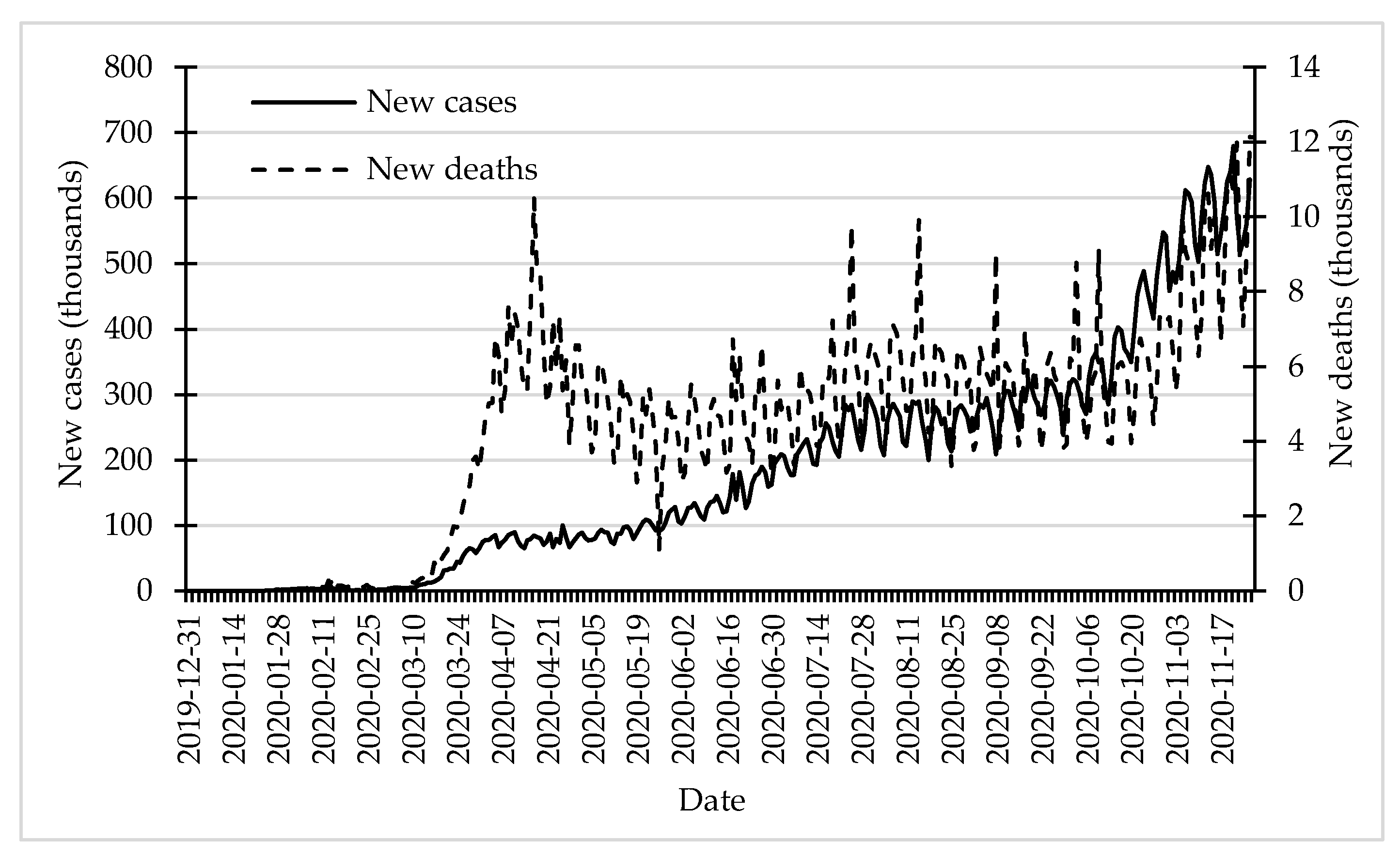
Although the first wave of the pandemic, that took place in spring 2020, had a higher fatality rate than the second wave that started at the beginning of October 2020, the second one had a much higher number of new infections. Although the fatality rate is lower, due to the larger number of cases, the total number of deaths is much higher (Figure 1).
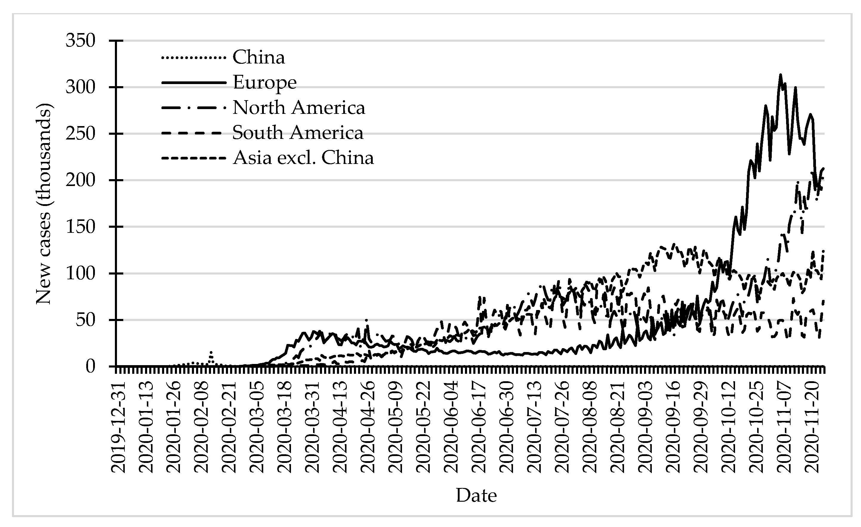
Geographical distribution of the spreading of the pandemic varied across the globe. At the beginning of the pandemic, the largest number of new cases was reported in China. In spring 2020, Europe became the centre of the pandemic. In the second half of spring, the number of new cases in Europe began to decrease, with increasing numbers in the Americas and Asia (excluding China). During mid-summer 2020, North America became the centre of the pandemic. In August and September, the largest numbers of new cases were reported in Asia. In mid-September, the number of new cases in Asia reported its peak. At the end of September, the second wave of the pandemic approached and hit Europe very hard. After about two weeks it also hit North America. In these two continents, the number of new infections started to grow rapidly. In Europe, it reached its peak on the 6th of November 2020, at the level of 313,500. North America reached its peak about two weeks later, at the level of almost 213,000 (Figure 2).
In his article, Fernandes (2020) characterised the main problems posed by the current global situation. They are:
- The pandemic is global;
- The world is much more globalised;
- Interest rates are historically low;
- It is not focused on low–middle income countries;
- Demand and supply are simultaneously devastated;
- It is generating spill-over effects throughout supply chains.
The aim of the study is to compare the intensity of decline and then increase in the value of basic stock indices during the SARS-CoV-2 coronavirus pandemic in 2020. The conducted research is a continuation of our previous analysis connected only with the decline in values of world stock indices. Our research presents the results of assessment of probability and intensity of increase in the values of stock indices after their previous decline. Moreover, obtained values are compared with previous results. We set the following research hypothesis:
Hypothesis 1.
The risk and intensity of the decline and then increase in stock indices varied on a continental level.
We verify the hypothesis by means of the survival analysis methods: Kaplan–Meier estimator, empirical hazard estimator, Cox proportional hazards model, and the logit model.
2. Selected Economic Aspects of the COVID-19 Pandemic
The outbreak of the pandemic results in significant adverse economic effects. Many countries have adopted a strict quarantine policy, which has significantly reduced the economic activity and caused mass unemployment. A particularly difficult situation is in sectors such as tourism and aviation. The exact global economic effect of the pandemic is not yet known, but the financial markets reacted with great strength. In ten days in March 2020, the US market hit the circuit breaker mechanism four times. It is worth noting that it was introduced in 1987 and since then it had been triggered just once, in 1997 (Zhang et al. 2020). The financial markets in Europe and Asia also plunged. On 12 March, the main stock index in the United Kingdom, FTSE, declined by over 10%. It was the worst day since 1987 (https://www.bbc.com/news/business-51829852 (accessed on 15 February 2021)). In March 2020, the Japanese stock market collapsed. The decline from the highest value in December 2019 was over 20% (https://www.bloomberg.com/news/articles/2020-03-09/perfect-storm-is-plunging-asia-stocks-to-bear-markets-one-by-one (accessed on 15 February 2021)). The central banks and authorities’ responses were immediate. These institutions introduced their policy instruments into the market. Most stock markets have recently begun to recover. However, with the progression of the pandemic, high uncertainty still persists (Ashraf 2020a).
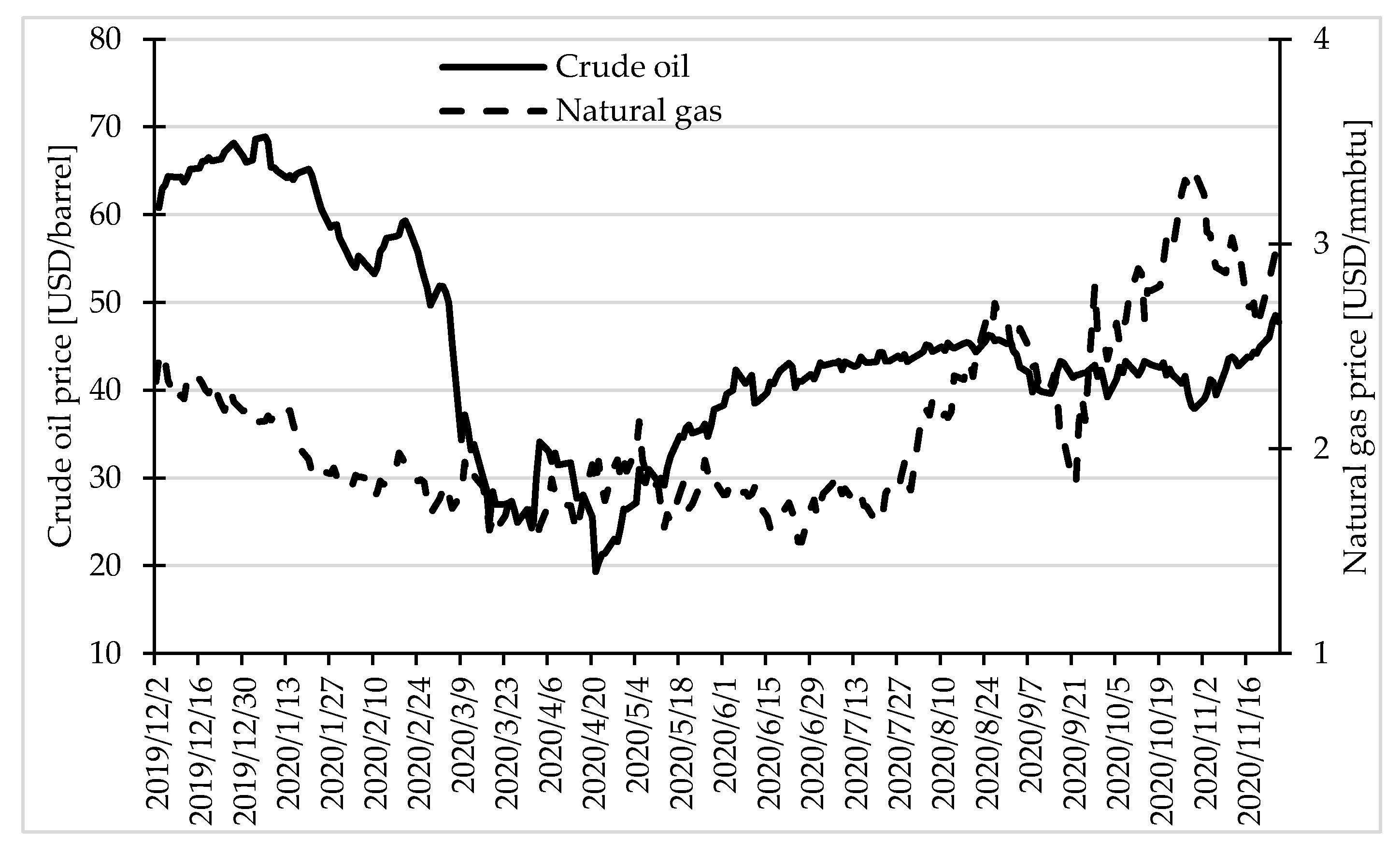
The pandemic influenced the global economy in many areas. However, the first symptoms of economic turbulence of any kind are usually noticeable first in financial markets. They manifest in changes of prices of commodities, such as fuels, metals, or agricultural products, and changes in values of stock indices. Figure 3 presents the changes of prices of selected fuels—crude oil and natural gas in the period 2 December 2019–26 November 2020.
At the beginning of the pandemic, the crude oil price was on its maximal level in the analysed period—almost 70 USD/barrel. When the pandemic became visible to the public, the crude oil price plunged from the level of almost 60 USD/barrel to below 20 USD/barrel. Then it began to regain its value, and after mid-July, it stabilised at the level between 40 and 50 USD/barrel. The course of the natural gas price was very much different. Since the beginning of the pandemic, it was slowly decreasing from the level of almost 2.5 USD per MMBtu to 1.5 USD/MMBtu on 2 April. Since that day, until the second half of July, it was stable at the level of 1.5–1.8. Then, the price of natural gas was increasing until the end of the observation period (26 November).
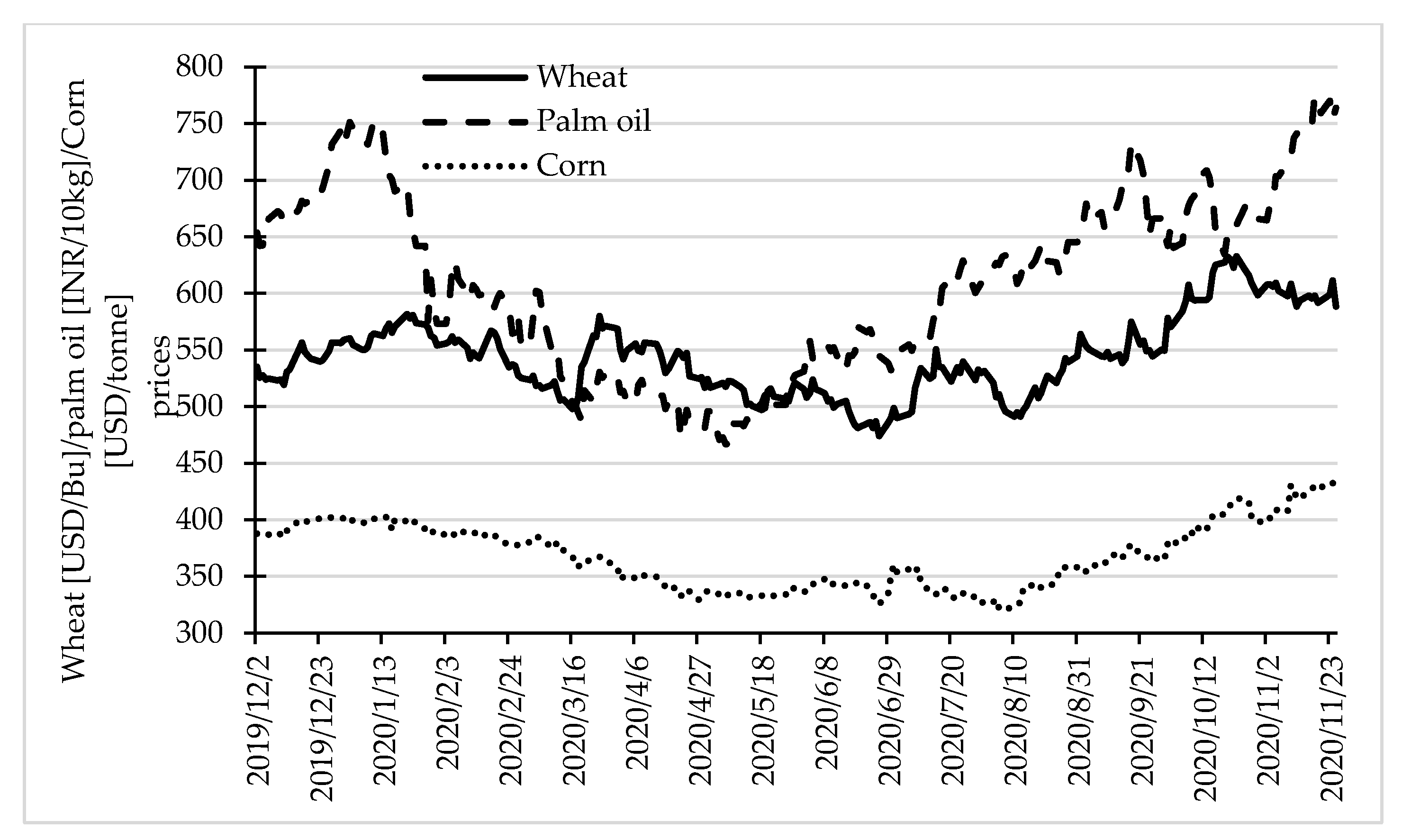
Prices of selected agricultural products (wheat, palm oil, and corn) had a different course. It seems that the declaration of the pandemic did not affect their trends. Prices of all three analysed commodities noted more or less constant decline since January 2020 until May 2020 (wheat and palm oil) or June (corn). Then they began to increase, and their increase was more or less constant (although with fluctuations) until the end of the observation period (Figure 4).
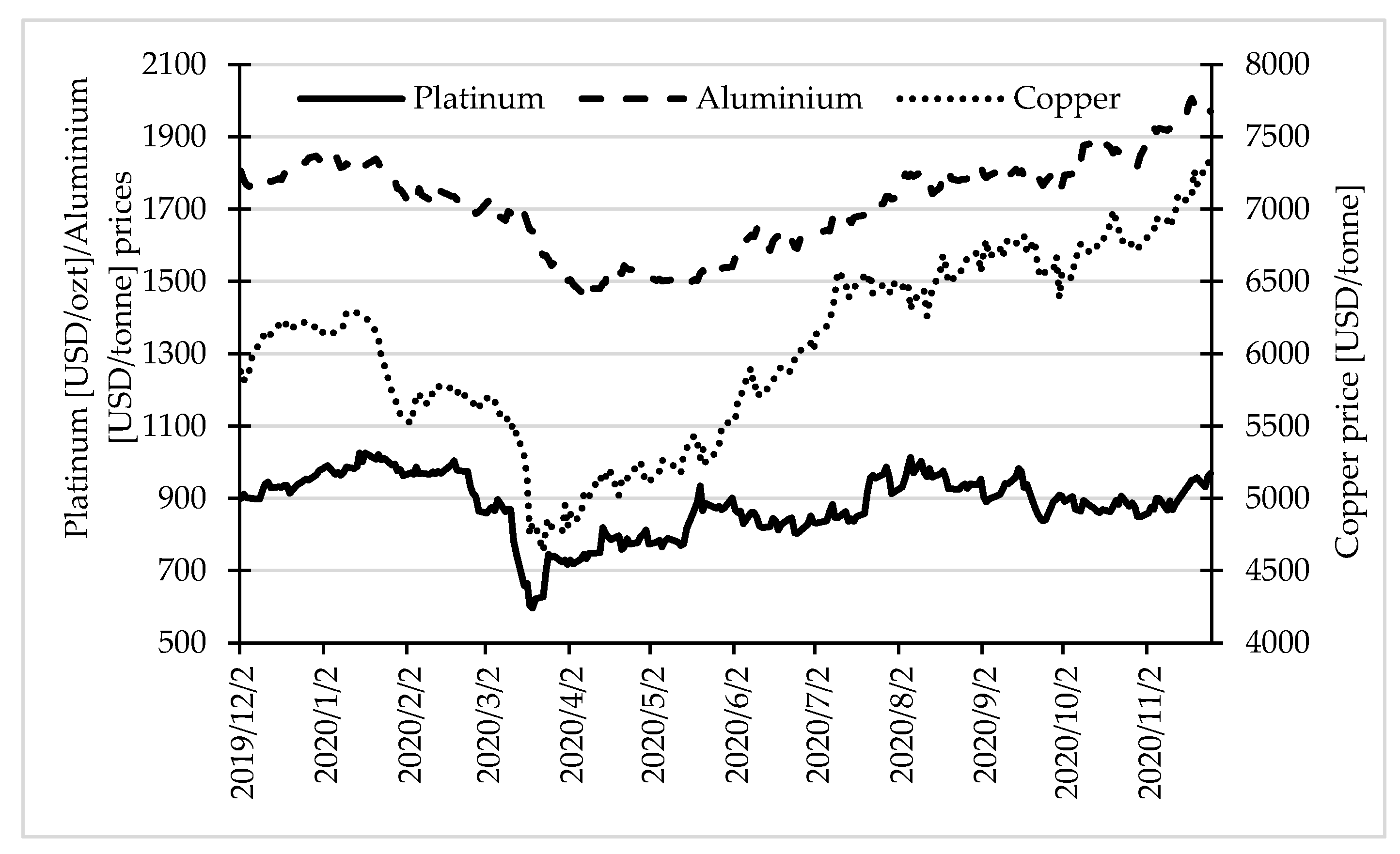
The last analysed group of commodities were selected metals (platinum, aluminium, and copper). Trends of prices of all of them were similar, although they had different magnitude. The prices were slightly increasing until mid-January and then began to decrease. After declaration of the pandemic, they noted a sharp decline. Since the end of March (beginning of April for aluminium), until the end of observation period (26 November), they were increasing, with the exception of the platinum price, which stabilised at the level of ca. 900 USD/ozt since mid-May until the end of the observation period (Figure 5).
It is also worth noting that the impact of the second wave of the pandemic is visible only in the case of prices of fuels, although it is much lower than in the first wave of the pandemic.
3. Literature Review
Since the beginning of the pandemic, medical and pharmaceutical research has been carried out in order to develop an effective vaccine and to develop methods of treating patients. At the same time, research is being carried out into the impact of the pandemic on the global economy and the methods of counteracting its effects.
Goodell (2020) compared the pandemic with other disasters that humanity faces. Local natural disasters affected only a certain area of the globe and primarily affect local financial markets. Climate change is too slow to consider its direct impact on the economy. The global nuclear crisis will quickly and effectively threaten the existence of entire humanity. The current pandemic can be seen as a global natural disaster.
Ashraf (2020b) applied available daily COVID-19 data and data referring to stock market returns from 64 countries in the period from 22 January 2020 until 17 April 2020 to analyse the influence of growth in COVID-19 confirmed cases and deaths on stock market returns. In his research, he considered country characteristics and systematic risk due to international factors. He found out that the reaction of the stock markets was particularly strong and resulted in negative returns with respect to the growth in confirmed COVID-19 cases. The stock markets’ response to the number of deaths was not statistically significant. He also showed that the strongest reaction of the stock markets was during the very beginning of the pandemic and then between 40 and 60 days after the initial confirmed cases.
Espinosa-Méndez and Arias (2020) analysed share prices of companies noted in the following indices: DAX 30 Index (Germany), CAC 40 (France), FTSE MIB (Italy), Ibex 35 Index (Spain), and FTSE 100 Index (United Kingdom) in the period since 3 January 2020 until 19 June 2020. They showed that the COVID-19 pandemic increased herding behaviour in European capital markets. Less aware investors followed the more aware in a clear example of herd behaviour. It subsequently caused erratic behaviour in the capital markets. Fear and uncertainty about the outcomes of the pandemic made less aware investors discard their confidence and follow the more aware ones.
Interesting studies on the influence of the pandemic on cryptocurrencies were conducted by Demir et al. (2020). They analysed the correlation between cryptocurrencies (Bitcoin (BTC), Ethereum (ETH), and Ripple (XRP)) and the COVID-19 cases/deaths. They applied the wavelet coherence analysis and initially noted a negative correlation between Bitcoin and the number of confirmed COVID-19 cases and deaths. Later, this correlation changed to positive. They obtained similar results for Ripple and Ethereum; however, the interactions were weaker. It showed the hedging role of cryptocurrencies against the uncertainty caused by COVID-19. The authors suggested that investors should have considered including cryptocurrencies in their portfolios depending on the COVID-19 phases. Cryptocurrencies would provide pandemic insurance benefits and could also be used as a payment and money transfer instrument.
Mazur et al. (2020) showed that the COVID-19 pandemic may not necessarily have been equally damaging to all companies and sectors. Although most sectors suffered and lost their values in the stock markets, others may have benefited from the pandemic and the ensuing lockdown. Healthcare, food, software stocks, and natural gas showed high positive returns. Equity values in real estate, entertainment, petroleum, and hospitality sectors plunged sharply.
Okorie and Lin (2020) confirmed the fractal contagion effect of the COVID-19 pandemic in the stock markets. They used the stock market information for the 32 biggest economies in the countries affected by the coronavirus (as of 31 March 2020). In addition, this fractal contagion effect disappeared over time (in the medium and long term) for both stock market returns and volatility. They confirmed a significant but short-term contagion effect in stock markets as a consequence of the COVID-19 pandemic. These contagion effects were found in both returns and stock market volatility.
Shear et al. (2021) in their study noted that increased investor attention to the COVID-19 pandemic resulted in negative stock market returns. This was particularly strong in countries where the investors held higher cultural values associated with avoiding uncertainty. They suggested that the investors’ cultural values associated with uncertainty avoidance promoted financial market volatility during the crisis.
Gunay et al. (2021) studied the influence of the first wave of the COVID-19 pandemic on various sectors of the Australian stock market. They showed that the pandemic mainly affected three sectors: consumer goods, industrials, and real estate. After accounting for company size, they found that smaller companies in the energy sector showed a gradual deterioration, while small companies in the consumer goods sector experienced the greatest positive impact of the pandemic.
The outbreak and quick spread of the COVID-19 pandemic hit global financial markets, including the energy sector. Czech and Wielechowski (2021) assessed the influence of the pandemic on stock indices connected with the conventional and alternative energy sectors. The analysed indices declined as the government anti-COVID-19 policy tightened, but the relationship was statistically significant only in the high variability regime. The alternative energy sector appeared to be more resilient to COVID-19 than the conventional one. It could suggest that COVID-19 had emphasised the growing concern about environmental pollution and climate change rather than depreciated them.
According to the definition of bullish (bearish) periods, there must have been a sufficiently large (at least 20%) decline/increase in a series of quotations. The study was based on the Dow theory (Rhea 1932), according to which the bearishness occurred when stock markets declined by 20%. Moreover, it was assumed that the phases of the stock market cycle (decline, increase, mid-range) should not last less than 4 months (Pagan and Sossounov 2003). Olbryś and Majewska (2015) applied the Pagan and Sossounov (2003) procedure for determining the periods of crisis. They analysed the monthly logarithmic rates of return of major stock exchange indices in Warsaw (WIG) and New York (S&P500) in the years 2007–2009. The possibilities of identifying a crisis depended on its type. Emin and Aytac (2016) presented 20 different definitions of the currency crisis. They used, inter alia, the studies by Reinhart and Rogoff (2009), who assumed that a currency crisis occurred when the currency value fell by at least 15% during a year in comparison with the value of the USD (or other currency adopted as a country’s reference).
Roszkowska and Prorokowski (2013) presented novel aspects and a broad picture of the financial crisis contagion, including the stages of contagion and the factors involved in its spread. They applied the modified Kaplan–Meier estimator. They proposed a model for the financial crisis contagion, which was based on international linkages between markets, with a focus on weaknesses in regulatory frameworks that allowed for the crisis to spread. Results of the simulation analysis (for the period 2007–2012) showed that Europe has experienced several phases of crisis contagion. Various regions and countries have been affected by different paths, propagated by different factors with not the same intensity. The diversity of vulnerability of European countries was evident both when comparing the developed markets with the emerging ones and within these groups.
We used the survival analysis methods in the research. Although they originate from demography and reliability theory, they are also widely used in social and economic research, including the financial market (Lunde and Timmermann 2004; Deville and Riva 2007; Markovitch and Golder 2008; Bieszk-Stolorz and Markowicz 2017a, 2018; Bieszk-Stolorz and Dmytrów 2021). It is applied, inter alia, to the analysis of the duration of companies and the analysis of crises.
Baschieri et al. (2020) investigated the role of initial capital structure on the success and duration of manufacturing start-ups entering the market. They used the survival analysis and focused on the period 2009–2016. Their analysis confirmed that the relationship between firm hazard and initial leverage was positive and significant also in case of the manufacturing companies in Italy. They also found weak evidence of a positive relationship between the quintiles of the leverage distribution and the hazard ratio.
Gepp and Kumar (2015) applied non-parametric classification and regression trees (CART) and a semi-parametric Cox model to prediction of difficult financial situations and compared the results obtained by both models. This analysis was carried out in relation to various cost indicators (Type I Error cost, Type II Error cost) and prediction intervals, as they were different depending on the situation. Obtained results showed that the survival analysis models and the decision trees had good prediction accuracy that justified their use and supported further examination.
By using the survival analysis methods, Deb (2006) presented the study on duration of recovery from a contractionary crisis. Most of the episodes of contraction were short lived. The recovery period for affected countries was two years after the recession caused by the crisis. Both the industrial and developing countries suffered from the contractionary crises. More frequent and severe contractions occurred for the Asian and the Latin American countries. In the research sample, these countries were responsible for two-thirds of the contractionary crises. It took them 4.5 years on average to recover. The average recovery time for other industrialised countries and developing ones was 2.8 and 2.4 years, respectively.
Puttachai et al. (2019) applied the Cox proportional hazards model to analyse which structural features might indicate that a country could be affected by a collapse in global GDP during the US financial crisis. They analysed 182 countries. Amongst them, 114 were not immune to the US financial crisis. The results from the Cox regression suggested that the developed economies, continents (Africa, Asia, and Australia), the human development, and the economic community (APEC and WTO) were the factors that provided a significant effect on the country’s survival during 2008–2009. The authors observed that the probability of survival decreased gradually after the 25th quarter and suddenly dropped in the 40th quarter, which corresponded to the US financial crisis.
Bieszk-Stolorz and Markowicz (2017b) applied the methods of the survival analysis for assessment of the variability of the shares of companies listed on the Warsaw Stock Exchange. They analysed the bear market in 2011 and the subsequent two years. They used the Kaplan–Meier estimator, the logit model, and the Cox regression model. They compared obtained results with previous ones for the 2008–2009 crisis. They examined 378 companies that were listed for the whole analysed period. They grouped them into three macro-sectors: finance, services, and industry. They confirmed the first hypothesis that the bear market in 2011 strongly affected the financial macro-sector. However, for the financial and industrial sectors, they did not confirm the second hypothesis—that the situation of macro-sectors during the financial crisis and the bear market was similar. The situation of the financial sector during the bear market was better than during the crisis, while for the industrial one it was worse.
4. Research Methodology
We applied the models and methods used in the survival analysis. They originate from demography and reliability theory. Their biggest development is connected with medical sciences, where it is commonly used for analysis of survival of patients. Currently, they are increasingly used in the analysis of socio-economic phenomena and are the basis of every study of the random variable T, describing survival time of analysed occurrence. Observations are carried out over a fixed period and the subject matter of the study are the individual units of a certain cohort. The parametric models are often used to analyse human life expectancy. It is because distributions such as Weibull, Gompertz, lognormal, and their mixtures describe human life expectancy well (Gompertz 1825). In the social-economic phenomena, the distribution of the survival time is usually unknown. It is the main reason for using the non-parametric and semiparametric methods. Another reason is that due to the relatively small number of observations, it would not be possible to estimate such a distribution, let alone fit a reliable parametric model. Their biggest advantage is the possibility of application of censored observations. For a specified observation period, some individuals may not experience the event before its termination and the duration may be known only partially. The presence of such units in the cohort significantly affects the total survival probability.
We assumed that the time a unit stays in a given state until a specific event occurs is a random variable T. In such a case, the cumulative distribution function F(t) expresses the probability that the event occurs until time t, at the latest. However, the basic concept in the survival analysis is the survival function, denoted by (Kleinbaum and Klein 2012):
where:
- T—duration,
- F(t)—cumulative distribution function of random variable T.
The survival function denotes the probability that a certain event will not occur until at least time t. Using Formula (1), we can determine the duration quartiles. These are the moments of time for which the survival function takes the following values: , , and , respectively. Because there are censored observations, not all quartiles can exist. This is because during the period of observation of the cohort, not all units experience the event (they still remain in the cohort).
The most widely used non-parametric estimator of the survival function is the Kaplan–Meier estimator. It is calculated by means of the following equation (Kaplan and Meier 1958):
where:
- ti—the point in time when at least one event occurs, ,
- di—number of events in time ti,
- ni—number of units observed in time ti, ,
- zi—number of censored observations in time ti.
We can determine the survival curve for all observations in general as well as for groups separated by unit characteristics. We can also compare such curves. There are many tests to investigate the significance of differences between two survival curves. We then verified the null hypothesis: . The alternative hypothesis can take one of the following forms: , or . We do not possess the consistent group of criteria to decide which test has the greatest power, thus which one should be used in the research. Some of them are more sensitive for the course of a survival curve in its initial part, while another one—in the final part. Latta (1981) proved that the power of tests depends on the sample size, censorship mechanism, and probability density of the hazard function. In 1972, the Peto brothers proposed modification of the Wilcoxon test. It is based on the estimation of the survival function, obtained by means of the Kaplan–Meier estimator for combined samples (Peto and Peto 1972). We used it when the hazard ratio between groups was not constant (Stevenson 2009). One of the assumptions of the Peto–Peto test is the same distribution of censored observations in both groups. Its main advantage, however, is that it does not lose power in the event of various types of censorship in groups. We should use this test if we want to pay more attention to initial parts of the survival curves.
The hazard function is the second important one in the survival analysis. It describes the intensity of occurrence of an event at time t under the condition of survival until time t and is denoted as follows (Kleinbaum and Klein 2012):
Depending on the analysed phenomenon, the hazard function allows us to assess the risk or chance of occurrence of an event at the moment t. In such a case, we often used the empirical hazard function, denoted by the following equation:
where:
- dj—the number of events in the j-th time interval,
- nj—the number of units observed in the j-th time interval,
- τj—the length of the j-th time interval.
We can assess hazard by estimation of the relative hazard (hazard ratio). For this purpose, we can use the semiparametric Cox hazards model, given by the following equation (Cox 1972):
where:
- —vector of independent variables,
- —baseline hazard,
- —model coefficients,
- t—observation period.
By means of this model, we can assess intensity of occurrence of an event at the moment t for the selected group with relation to the reference group. In this purpose, we do not use parameters directly, but we calculated the hazard ratios, by means of the formula .
We can assess the relative chance/risk (odds ratio) of an event by means of a logit model (Kleinbaum and Klein 2010):
where:
- —conditional probability of the occurrence of an event,
- —vector of independent variables,
- —model coefficients.
Model (6) is a discrete time model using logistic regression for the entire period (Cox 1972, p. 192). The variable Y takes the value 1 if the event occurred and 0 if the event did not occur during the observation period (censored observation).
The coefficients of the logit model allow us to determine the chance (odds/risk) that an event occurs at the moment t in the selected group in relation to the reference group. Moreover, in this case we do not analyse the parameters directly, but the relative risk, denoted by the formula .
5. Statistical Data and Basic Assumptions of the Research
We used a cohort of 108 of the most important stock market indices. They are presented in Table A1 in Appendix A. We observed the values of the indices from mid-December 2019 until 15 July 2020. We analysed the two phenomena—decline in the value of the indices and then their increase. In the case of the first one, we analysed 20% decline in the value of the indices from their maximal value. For these reasons, we observed the stock exchange indices from mid-December 2019 to mid-April 2020 (4 months). We considered the moment when the analysed index reached its maximum during the observation period as an initial event. The moment when the index recorded a 20% decline from its maximal value, we considered as the final event. In such a case, the random variable T was the time that elapsed between the initial and the final event. The next analysed phenomenon was the 20% increase in the values of the indices. In this case, the random variable T was the time that elapsed from the minimum value (initial event) until the moment of reaching the 20% increase of the value (final event). Due to the process of the spreading the pandemic, we grouped the indices by continents. By doing this, we selected four groups of indices: European, American, African, and Asian plus Australian ones. Because of the fact that we analysed only three indices for Australia and New Zealand, we decided to add them to the Asian ones. In the analysed period, not all the indices have reached the assumed limit values. These are the censored observations. Table 1 presents the share of indices for each group that reached at least a 20% decline in their values, a 20% increase, and those that did not reach the assumed limit values. Additionally, Table 1 presents maximal and minimal times of decline and increase in values of the indices. The first required decline took place on the 19th day since maximal value (in Europe) and the last one—on the 84th day (also in Europe). Twenty percent of indices did not record the required decline in their values—the largest number of them was in Africa (44%). The first required increase took place on the third day after the minimal value (in America and Africa) and the last one—on the 106th day (Asia + Australia). Thirty percent of indices did not record the required 20% increase in their values. Furthermore, in this case, the largest share of them was in Africa.
6. Empirical Research and Discussion
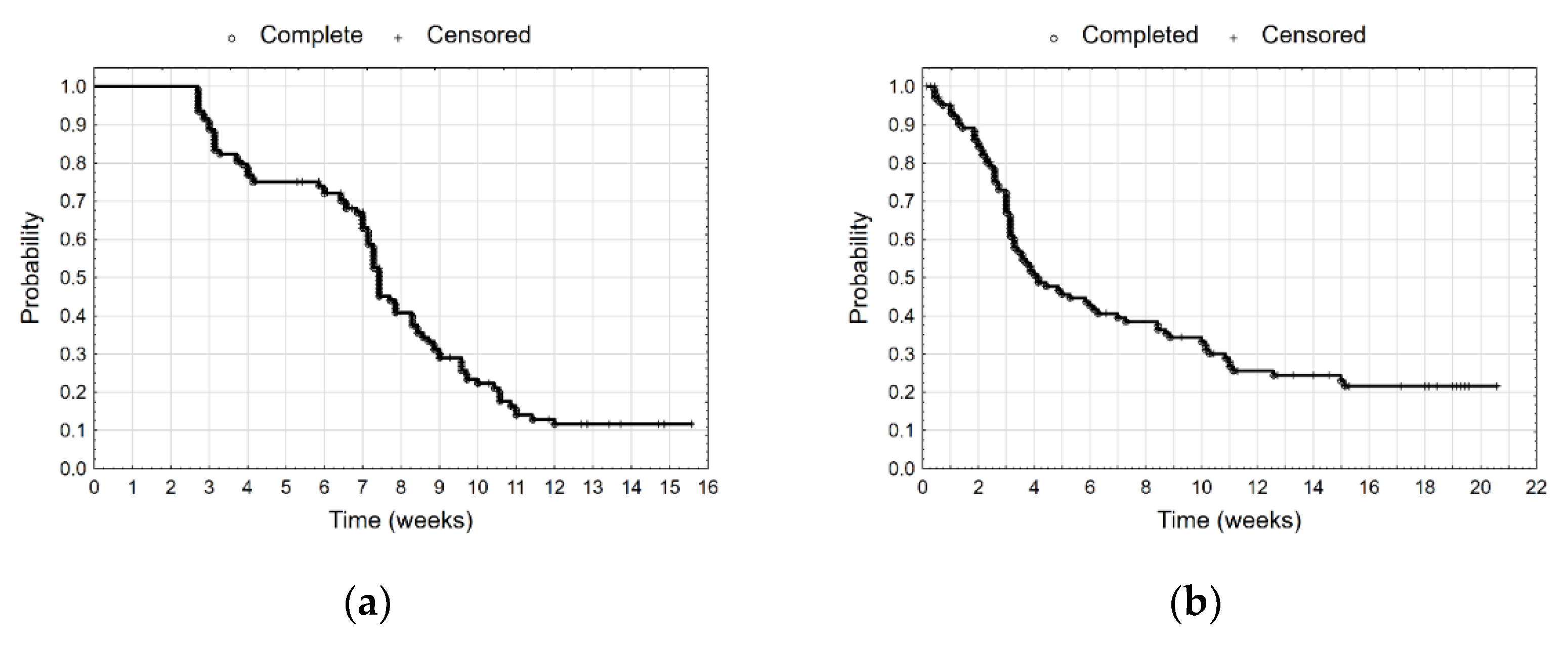
All calculations were performed in Statistica 13.3 and Microsoft Excel for Microsoft 365 software. In the first stage of the research, we used the Kaplan–Meier estimator for assessment of probability of not reaching the 20% decline and then 20% increase in value of the stock indices. At first, we analysed all the indices together. We recorded the first 20% decrease on the 19th day from the moment the maximal value was reached (Figure 6a). On the other hand, we observed the first increase after the third day from the minimal value (Figure 6b). The median duration of the 20% decline in values of indices was 52 days. That means that half of the indices recorded a 20% decline within 52 days after reaching their maximal value. Likewise, the median duration for the 20% increase in values of the indices after their minimum was 29 days.
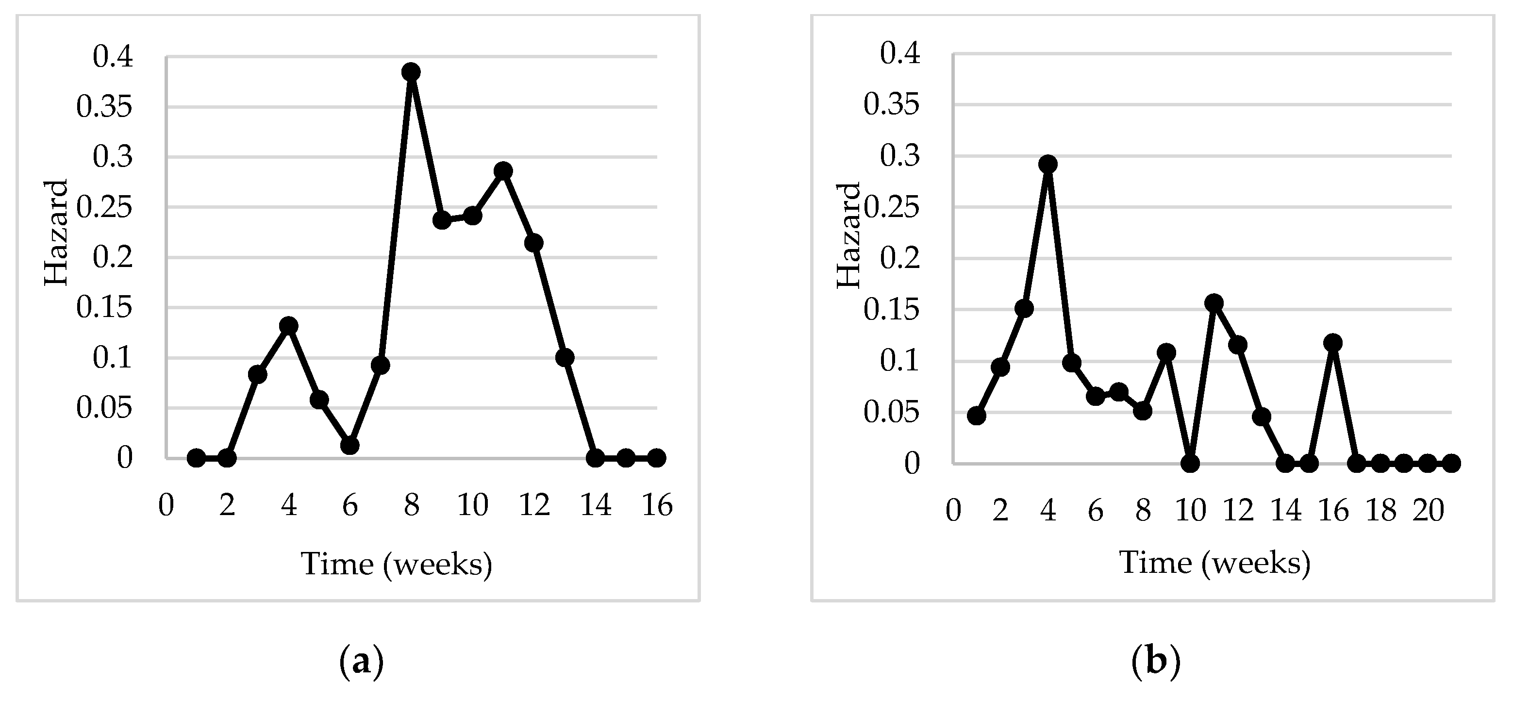
We then estimated the empirical hazard estimator for all indices together. We assessed the intensity of a 20% decline and increase in values of the stock market indices. The highest intensity of the decline in the indices was in the fourth and eighth weeks (Figure 7a). The hazard function has local maxima at these two points. It is confirmed by the Kaplan–Meier estimator (Figure 6a). Between the third and fourth week and seventh and eighth week, it has a significantly higher decline in its value. The highest intensity of the increase in the indices was in the fourth and eleventh week (Figure 7b). That means that between the third and fourth week, the Kaplan–Meier estimator has a significantly higher decline in its value (Figure 6b).
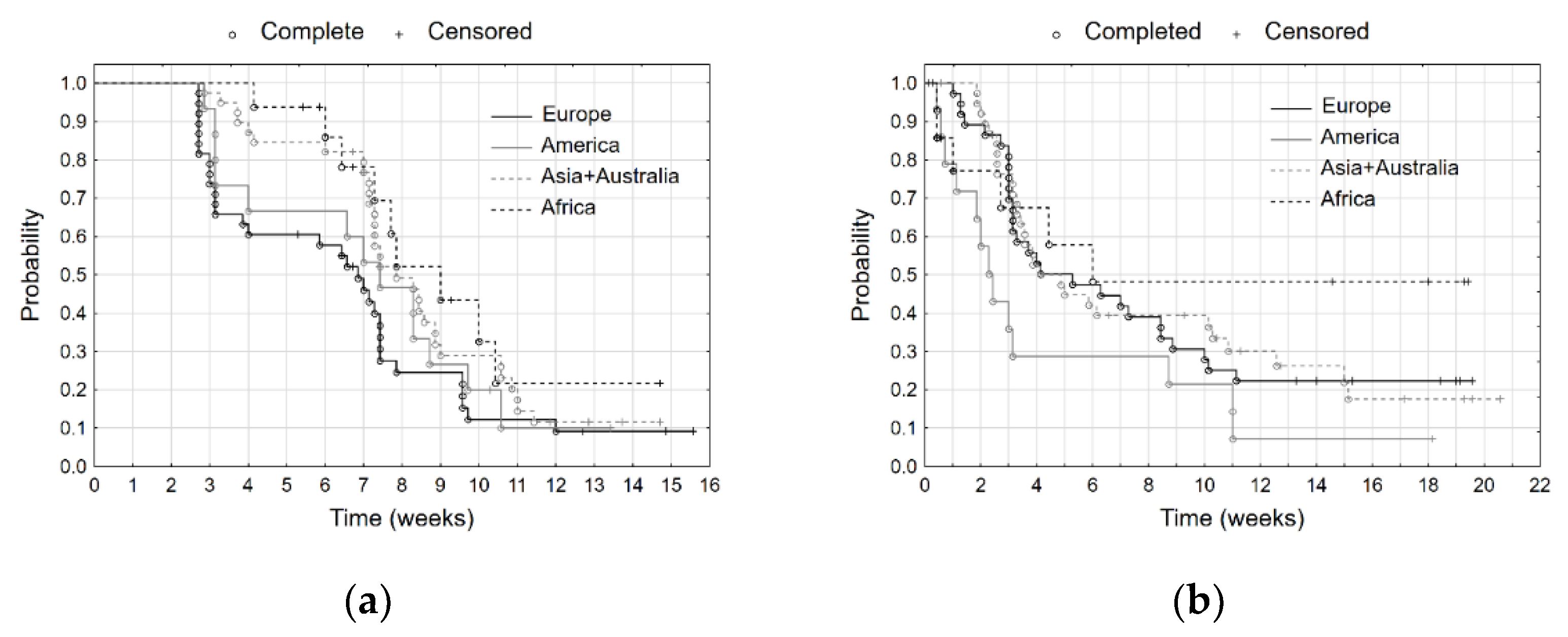
In the next stage of the research, we determined the Kaplan–Meier estimators for the groups of indices. These groups were distinguished by their continental belonging (Figure 8). The European stock exchanges recorded the fastest 20% decline in the indices. They were followed by the American, and Asian with Australian ones. The slowest decline in values of the stock market indices was recorded in Africa. We can confirm this by analysing the mutual position of the survival curves (Figure 8a). In the next step, we analysed the increase in the values of the stock market indices. The fastest increase from their minimal values was observed for the American indices. Increases in values of European, Asian, and Australian stock indices were similar, while in case of the African ones, the increase was the slowest.
We compared the survival curves by means of the Peto–Peto test (Table 2). For the decline in the values of the stock market indices, we confirmed the significance of differences between many groups (at a level of 0.05). We examined separately every pair of groups. We rejected the null hypothesis of the equality of survival curves (at a 0.01 significance level) for pairs: Europe and Africa and for Europe and Asia + Australia. When we analysed the increase in values of the stock market indices, the test indicates differences between curves at a significance level of 0.1. The test for pairs of continents shows significant difference (at a 0.05 significance level) only in the case of pair America and Asia + Australia.
On the basis of the survival curves for all indices together and by continents, we calculated the quartiles of duration (Table 3). In the case of the decline in values of stock indices, the first quartiles for Europe and America (21 and 22 days, respectively) show faster and similar rates of decline. The pair Asia with Australia and Africa had similar, but much slower rates (50 and 51 days, respectively). By the time in which 75% of the European indices recorded at least 20% decline (55 days) in their values, such decrease was observed for half of Asian and Australian ones. By this time, a little more than 25% of the African stock market indices recorded required decline. When we analysed the increase in the values of the indices, it turns out that in the case of Africa the rate of increase at the beginning was fast (first quartile was equal to 10 days), but in the subsequent period it was slower (median equal to 40 days). The lack of the third quartile informs that until the end of observation period, less than 75% of indices recorded a 20% increase in their values. The values of the quartiles for America (7, 16, 42 days) show a faster rate of increase in the values of stock indices. The values of the first quartiles for Europe and Asia + Australia (21 and 20 days for the first quartile, 30 and 29 days for median) show a similar and slower rate of decline of stock indices.
In the last stage of our research, we analysed the relative hazard and the relative risk of decline and increase in the values of indices across continents. We determined this decline/increase with respect to the geographical location (continent) of the index (xi). This qualitative variable was converted into dummy (dichotomous) variables. With accordance to the rules of econometric modelling, the number of dummy variables must be one less than the number of categories. We considered the African indices as a reference group (coded as 0). Previous analysis proved that this was the continent where the decline and increase in the values of indices were the slowest. Therefore, we obtained the three variables in the models: x1 (Europe), x2 (America), x3 (Asia + Australia). We assumed that the threshold value for the decline/increase was 20%. In the case of the logit model, the dichotomous explained variable Y takes the value of 1 if there is at least a 20% decline/increase in the values of indices, and the value of 0 otherwise. We assessed the relative hazard (relative intensity) of a 20% decline and increase in the values of the stock market indices by means of the Cox proportional hazard model. We used the logit model to assess a relative risk/chance of a 20% decline and increase in the values of the stock market indices. We present the results of the parameter estimation of the Cox hazards and the logit models in Table 4.
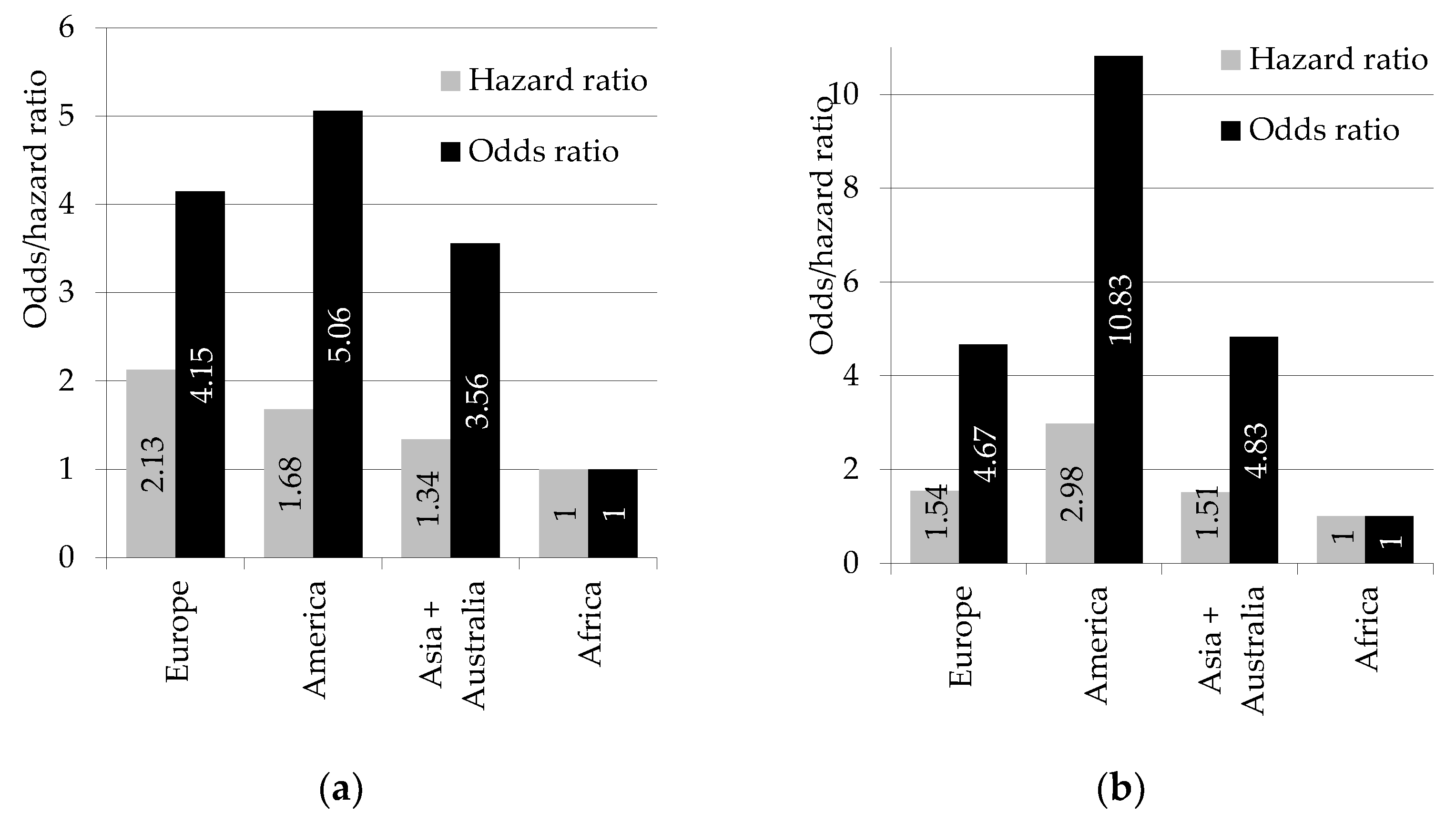
We present the hazard/odds ratios in Figure 9. If their value is above 1, it means that an intensity or risk of decline/increase is higher than for Africa. For both situations (decline and increase), all the hazard and odds ratios are greater than 1. For Africa alone, as a reference group, they are equal to 1.
The intensity of decline for the European indices was the highest and 2.13 times higher than for Africa. The American indices had a 1.68 times higher intensity of decline than the African ones. For the Asian and Australian ones, this intensity was 1.34 times higher than for the reference group. The risk of decline in values of indices was the highest on the American exchanges—about 5 times higher than for the African ones, for the European stock exchanges it was 4.15 times higher, and for Asian and Australian ones—3.56 times higher. This means that the European and American markets reacted the most forcefully to the pandemic situation.
The increase intensity of the American indices was the highest and 2.98 times higher than for African ones; for the European indices it was 1.54 times, and for the Asian and Australian ones—1.51 times higher. The risk of increase in values of indices was the highest in the American exchanges and about 10.83 times higher than for the African ones. For the Asian and Australian stock exchanges it was 4.83 times higher, and for the European stock exchanges—4.67 times higher. This means that for the European and Asian and Australian markets, increases of the indices from their minimal values were similar.
This study confirms the results obtained by Singh et al. (2020). They analysed the impact of the COVID-19 pandemic on the stock market in a sample of G-20 countries. They showed that after the outbreak, stock markets around the world behaved badly and achieved negative returns. However, the markets gradually recovered in the later stages. The regression results of the panel data provide evidence to support the recovery of the stock market after the negative impact of COVID-19. The implication is that the future uncertainty associated with the outbreak initially caused panic sales in stock markets around the world. H. Liu et al. (2020) found that the main explanation for the initial panic in the financial markets was the actions taken by governments, such as closing offices and factories and reducing activity, which resulted in a reduction in labour force, productivity, and consequently corporate profitability. The weaker response of emerging market stock markets to the pandemic is explained by the research of Topcu and Gulal (2020), who showed that their governments took the required actions in time and announced larger stimulus packages. Chowdhury et al. (2021) analysed panel data from 12 countries covering four continents from January to April 2020. They used each country’s stock market index, purchasing managers’ index, and variables characterising the course of the pandemic: restriction in internal movement, the number of lockdown days, restriction in international travel, confirmed cases, and fiscal measures. They observed a severe negative impact of the pandemic on stock market returns. European stock markets were the most affected in comparison to others in the initial phase of the pandemic.
In the study, we analysed the first wave of the pandemic. The variation in the impact of a pandemic on stock indices is related to its spread and scale. There are theories linking the development of pandemics to climatic and weather conditions. The frequency of respiratory virus infections is usually seasonal. This is also true for COVID-19. Moderately cool and dry weather, high pressure, low-speed winds, and moderate rainfall are conducive to this type of illness. Such a situation occurred from January to March 2020 in both Wuhan and northern Italy. Similar weather conditions occurred in other countries where large numbers of infections were observed, such as Western Europe and the United States. These regions had similar weather conditions during this period. Studies by many authors (Scafetta 2020; Tzampoglou and Loukidis 2020; Spena et al. 2020; Haque and Rahman 2020; Wang et al. 2021; J. Liu et al. 2020; Tobías and Molina 2020) confirm the negative impact of high temperature and high humidity on the number of infections and pandemic deaths. They suggest that the pandemic is likely to evolve in line with the seasonal temperature cycle. This was indicated by the migration of the infection wave from the northern to the southern hemisphere. The southern hemisphere appears to be more protected as most of its surface area, with the exception of a few regions, is always warm enough throughout the year. Moreover, the relatively low median age of the population in African countries may contribute to pandemic mitigation there. Based on the weather model, the authors suggested a second wave of infections in the northern hemisphere in the autumn of 2020. This is what happened. This phenomenon can explain the delayed decline in African and Asian stock indices.
7. Conclusions
Our research confirms that the stock markets responded to the SARS-CoV-2 coronavirus pandemic in various ways. The 20% decline in the value of stock indices occurred in 80% of the stock exchanges analysed. It shows that value drops for all stock exchanges, showing an almost simultaneous reaction to the spread of the virus. On the other hand, a 20% increase from their minimal values was visible for 70% of stock indices. The data analysis indicates that the moment when the maximal value of indices was recorded was different for individual stock exchanges. However, the largest drops occurred in March 2020. This happened after the declaration of the pandemic state by the WHO (11 March 2020). It caused the differences in risk and intensity of decline in the values of indices for various countries and continents. The American stock exchanges have the greatest risk of decline and increase. This is because 87% of the American indices lost and then gained 20% of their value. The American stock exchanges have also the highest intensity of increases in the values of indices. We observed that the European exchanges have the highest intensity of decline, which results from the fact that there was the shortest time of fall from the maximum value (median duration equal to 48 days) with a high percentage of indices that reached the required limit. We can explain this phenomenon by the fact that the European countries (especially Italy and the United Kingdom) were struck by the first wave of the pandemic very hard and earlier than the countries on the American continent. The European and Asian plus Australian stock markets have similar intensity and chance for increase in the values of indices. During the first wave of the pandemic, we observed the lowest or no index declines in the African countries. Africa is also distinguished by the fact that when analysing increases in the values of the stock indices, most of them (62%) did not record a 20% increase. This confirms the research hypothesis that both decline and then increase in the values of the stock indices varied on the continental level.
We plan to carry out a similar analysis in the future in connection with subsequent pandemic waves and using other research methods as well. It is also interesting to examine and compare the behaviour of sectoral indices.
Author Contributions
Conceptualisation, B.B.-S. and K.D.; methodology, B.B.-S. and K.D.; software, B.B.-S.; validation, K.D.; formal analysis, B.B.-S.; investigation, B.B.-S. and K.D.; resources, B.B.-S. and K.D.; writing—original draft preparation, B.B.-S. and K.D.; writing—review and editing, K.D. All authors have read and agreed to the published version of the manuscript.
Funding
This research received no external funding.
Data Availability Statement
The data referring to the COVID-19 cases was downloaded from the https://ourworldindata.org/coronavirus-source-data (accessed on 27 November 2020) webpage. Data referring to the analysed stock indices was downloaded from the https://stooq.pl (accessed on 1 September 2020) financial service.
Acknowledgments
The authors would like to thank the anonymous reviewers for their valuable feedback and suggestions, which were helpful in further improving the commentary.
Conflicts of Interest
The authors declare no conflict of interest.
Appendix A

Table A1.
Stock indices used in the study. Source: own elaboration.
| Country | Index | Country | Index | Country | Index |
|---|---|---|---|---|---|
| Argentina | MERVAL | Ireland | ISEQ | Russia | MOEX |
| Australia | S&P/ASX200 | Israel | TA35 | Russia | RTS |
| Austria | ATX | Italy | FTSEMIB | Rwanda | ALSIRW |
| Bahrain | Bahrain All Share | Ivory Coast | BRVM10 | Saudi Arabia | MSCI TADAWUL 30 |
| Bangladesh | DSE30 | Jamaica | JSEMI | Saudi Arabia | TASI |
| Belgium | BEL20 | Japan | NIKKEI | Serbia | BELEX15 |
| Bosnia and Herzegovina | BIRS1 | Jordan | AMGNRLX | Singapore | STI |
| Bosnia and Herzegovina | SARAJEVO10 | Kazakhstan | KASE | Slovakia | SAX |
| Botswana | BSE | Kenya | NSE20 | Slovenia | SBITOP |
| Brazil | BOVESPA | Lebanon | BLSI | South Korea | KOSPI |
| Bulgaria | BSE SOFIX | Malaysia | KLCI | South Korea | KS50 |
| Canada | TSX | Malta | MSE | Spain | IBEX35 |
| Chile | SASEIPSA | Mauritius | MDEX | Sri Lanka | CSE |
| China | SSECOMP | Mexico | BMV | Sweden | OMXS30 |
| China | SZSECOMP | Mexico | FTFTBIVA | Switzerland | SSMI |
| Columbia | COLCAP | Mongolia | MNETOP20 | Thailand | SETI |
| Croatia | CROBEX | Montenegro | MNSE10 | Taiwan | GTSM50 |
| Cyprus | Cyprus Main Market | Morocco | MASI | Taiwan | TAIEX |
| Czechia | PX | Namibia | FTN098 | Tanzania | DSEI |
| Denmark | OMXC20 | Netherlands | AEX | Tunisia | TUNINDEX |
| Ecuador | Guayaquil Select | New Zealand | NZMC | Tunisia | TUNINDEX20 |
| Egypt | EGX30 | New Zealand | NZX50 | Turkey | BIST100 |
| Egypt | EGX70 | Nigeria | NGSE30 | UAE | ADXGENERAL |
| Finland | OMXH25 | Norway | OBX | UAE | DFMGI |
| France | CAC40 | Norway | OSEBX | Uganda | ALSIUG |
| Germany | DAX | Oman | MSI | Ukraine | PFTSI |
| Germany | STOXX50E | Pakistan | KSE | United Kingdom | FTSE |
| Greece | THEXCOMP | Peru | SPBLPGPT | USA | DJI |
| Hong Kong | FTXIN25 | Philippines | PSEICOMP | USA | NASDAQ |
| Hong Kong | HANGSENG | PNA | PLE | USA | NDX |
| Hungary | BUX | Poland | WIG20 | USA | SP500 |
| Iceland | OMXIPI | Poland | WIG30 | Venezuela | IBC |
| India | NSEI | Portugal | PSI20 | Vietnam | HNX30 |
| India | SENSEX | Qatar | QSI | Vietnam | VNI |
| Indonesia | IDXCOMP | Romania | BETI | Vietnam | VNI30 |
| Iraq | ISX60 | RSA | JTOPI | Zambia | LASILZ |
References
- Ashraf, Badar N. 2020a. Economic impact of government interventions during the COVID-19 pandemic: International evidence from financial markets. Journal of Behavioral and Experimental Finance 27: 100371. [Google Scholar] [CrossRef] [PubMed]
- Ashraf, Badar N. 2020b. Stock markets’ reaction to COVID-19: Cases or fatalities? Research in International Business and Finance 54: 101249. [Google Scholar] [CrossRef]
- Baschieri, Giulia, Giorgio S. Bertinetti, and Gloria Gardenal. 2020. Start-Ups Beyond the Crisis: A Survival Analysis. In Banking and Beyond. Palgrave Macmillan Studies in Banking and Financial Institutions. Edited by Caterina Cruciani, Gloria Gardenal and Elisa Cavezzali. Cham: Palgrave Macmillan, pp. 237–56. [Google Scholar] [CrossRef]
- Bieszk-Stolorz, Beata, and Krzysztof Dmytrów. 2021. A survival analysis in the assessment of the influence of the SARS-CoV-2 pandemic on the probability and intensity of decline in the value of stock indices. Eurasian Economic Review 11: 363–379. [Google Scholar] [CrossRef]
- Bieszk-Stolorz, Beata, and Iwona Markowicz. 2017a. Methods of Event History Analysis in the Assessment of Crisis Impact on Sectors Related with the Real Estate Market in Poland. Folia Oeconomica Stetinensia 17: 57–67. [Google Scholar] [CrossRef] [Green Version]
- Bieszk-Stolorz, Beata, and Iwona Markowicz. 2017b. The assessment of the situation of listed companies in macrosectors in a bear market—Duration analysis models. In 20-th AMSE. Applications of Mathematics and Statistics in Economics. International Scientific Conference: Szklarska Poręba, 30 August–3 September 2017. Conference Proceedings Full Text Papers. Edited by Albert Gardoń, Cyprian Kozyra and Edyta Mazurek. Wrocław: Wydawnictwo Uniwersytetu Ekonomicznego we Wrocławiu, pp. 17–25. [Google Scholar] [CrossRef] [Green Version]
- Bieszk-Stolorz, Beata, and Iwona Markowicz. 2018. Application of models of survival analysis in the assessment of the situation of macrosectors of listed companies. Optimum. Economic Studies 1: 3–15. [Google Scholar] [CrossRef] [Green Version]
- Chowdhury, Emon K., Iffat I. Khan, and Bablu K. Dhar. 2021. Catastrophic impact of Covid-19 on the global stock markets and economic activities. Business and Society Review. [Google Scholar] [CrossRef]
- Cox, David R. 1972. Regression Models and Life-Tables. Journal of the Royal Statistical Society, Series B (Methodological) 34: 187–220. [Google Scholar] [CrossRef]
- Czech, Katarzyna, and Michał Wielechowski. 2021. Is the Alternative Energy Sector COVID-19 Resistant? Comparison with the Conventional Energy Sector: Markov-Switching Model Analysis of Stock Market Indices of Energy Companies. Energies 14: 988. [Google Scholar] [CrossRef]
- Deb, Saubnik. 2006. Trade First and Trade Fast: A Duration Analysis of Recovery from Currency Crisis. Departmental Working Paper 2006-07. New Brunswick: Department of Economics, Rutgers University. [Google Scholar]
- Demir, Ender, Mehmet H. Bilgin, Gokan Karabulut, and Asli C. Doker. 2020. The relationship between cryptocurrencies and COVID-19 Pandemic. Eurasian Economic Review 10: 349–60. [Google Scholar] [CrossRef]
- Deville, Laurent, and Fabrice Riva. 2007. Liquidity and Arbitrage in Options Markets: A Survival Analysis Approach. Review of Finance 11: 497–525. [Google Scholar] [CrossRef] [Green Version]
- Emin, Dogus, and Aysegul Aytac. 2016. The challenge of predicting currency crises: How do definition and probability threshold choice make a difference? Eurasian Economic Review 6: 195–213. [Google Scholar] [CrossRef] [Green Version]
- Espinosa-Méndez, Christian, and Jose Arias. 2020. COVID-19 effect on herding behaviour in European capital markets. Finance Research Letters 38: 101787. [Google Scholar] [CrossRef] [PubMed]
- Fernandes, Nuno. 2020. Economic effects of coronavirus outbreak (COVID-19) on the world economy. IESE Business School Working Paper No. WP-1240-E. [Google Scholar] [CrossRef]
- Gepp, Adrian, and Kuldeep Kumar. 2015. Predicting Financial Distress: A Comparison of Survival Analysis and Decision Tree Techniques. Procedia Computer Science 54: 396–404. [Google Scholar] [CrossRef] [Green Version]
- Gompertz, Benjamin. 1825. On the nature of the function expressive of the law of human mortality, and on a new mode of determining the value of life contingencies. Philosophical Transactions of the Royal Society of London 115: 513–83. [Google Scholar]
- Goodell, John W. 2020. COVID-19 and finance: Agendas for future research. Finance Research Letters 35: 101512. [Google Scholar] [CrossRef] [PubMed]
- Gunay, Samet, Walid Bakry, and Somar Al-Mohamad. 2021. The Australian Stock Market’s Reaction to the First Wave of the COVID-19 Pandemic and Black Summer Bushfires: A Sectoral Analysis. Journal of Risk and Financial Management 14: 175. [Google Scholar] [CrossRef]
- Haque, Syed Emdadul, and Mosiur Rahman. 2020. Association between Temperature, Humidity, and COVID-19 Outbreaks in Bangladesh. Environmental Science & Policy 114: 253–55. [Google Scholar] [CrossRef]
- Kaplan, Edward L., and Paul Meier. 1958. Nonparametric estimation from incomplete observations. Journal of the American Statistical Association 53: 457–81. [Google Scholar] [CrossRef]
- Kleinbaum, David G., and Mitchel Klein. 2010. Logistic Regression. A Self-Learning Text, 3rd ed. New York: Springer. [Google Scholar] [CrossRef]
- Kleinbaum, David G., and Mitchel Klein. 2012. Survival Analysis. A Self-Learning Text, 3rd ed. New York: Springer. [Google Scholar] [CrossRef]
- Latta, Robert B. 1981. A Monte Carlo study of some two-sample rank tests with censored data. Journal of the American Statistical Association 76: 713–19. [Google Scholar] [CrossRef]
- Liu, HaiYue, Aqsa Manzoor, CangYu Wang, Lei Zhang, and Zaira Manzoor. 2020. The COVID-19 Outbreak and Affected Countries Stock Markets Response. International Journal of Environmental Research and Public Health 17: 2800. [Google Scholar] [CrossRef] [Green Version]
- Liu, Jiangtao, Ji Zhou, Jinxi Yao, Xiuxia Zhang, Lanyu Li, Xiaocheng Xu, Xiaotao He, Bo Wang, Shihua Fu, Tingting Niu, and et al. 2020. Impact of Meteorological Factors on the COVID-19 Transmission: A Multi-City Study in China. Science of The Total Environment 726: 138513. [Google Scholar] [CrossRef]
- Lunde, Asger, and Allan Timmermann. 2004. Duration Dependence in Stock Prices: An Analysis of Bull and Bear Markets. Journal of Business & Economic Statistics 22: 253–73. [Google Scholar] [CrossRef] [Green Version]
- Markovitch, Dmitri G., and Peter N. Golder. 2008. Findings—Using Stock Prices to Predict Market Events: Evidence on Sales Takeoff and Long-Term Firm Survival. Marketing Science 27: 717–29. [Google Scholar] [CrossRef] [Green Version]
- Mazur, Mieszko, Man Dang, and Miguel Vega. 2020. COVID-19 and the march 2020 stock market crash. Evidence from S&P1500. Finance Research Letters 38: 101690. [Google Scholar] [CrossRef]
- Okorie, David I., and Boqiang Lin. 2020. Stock markets and the COVID-19 fractal contagion effects. Finance Research Letters 38: 101640. [Google Scholar] [CrossRef]
- Olbryś, Joanna, and Elżbieta Majewska. 2015. Bear Market Periods During the 2007–2009 Financial Crisis: Direct Evidence from the Visegrad Countries. Acta Oeconomica 65: 547–65. [Google Scholar] [CrossRef]
- Pagan, Adrian R., and Kirill A. Sossounov. 2003. A Simple Framework for Analysing Bull and Bear Markets. Journal of Applied Economics 18: 23–46. [Google Scholar] [CrossRef]
- Peto, Richard, and Julian Peto. 1972. Asymptotically efficient rank invariant test procedures. Journal of the Royal Statistical Society: Series A (Statistics in Society) 135: 185–207. [Google Scholar] [CrossRef]
- Puttachai, Wachirawit, Woraphon Yamaka, Paravee Maneejuk, and Songsak Sriboonchitta. 2019. Analysis of the Global Economic Crisis Using the Cox Proportional Hazards Model. In Beyond Traditional Probabilistic Methods in Economics. ECONVN 2019 Studies in Computational Intelligence. Edited by Vladik Kreinovich, Nguyen Ngoc Thach, Nguyen Duc Trung and Dang Van Thanh. Cham: Springer, vol. 809, pp. 863–72. [Google Scholar] [CrossRef]
- Reinhart, Carmen M., and Kenneth S. Rogoff. 2009. This Time is Different: A Panoramic View of Eight Centuries of Financial Crises. NBER Working Paper Series 13882. Available online: https://0-doi-org.brum.beds.ac.uk/10.3386/w13882 (accessed on 15 February 2021).
- Rhea, Robert. 1932. The Dow Theory. New York: Barron’s. [Google Scholar]
- Roszkowska, Paulina, and Łukasz Prorokowski. 2013. Model of Financial Crisis Contagion: A survey-based Simulation by Means of the Modified Kaplan-Meier Survival Plots. Folia Oeconomica Stetinenesia 13: 22–55. [Google Scholar] [CrossRef]
- Scafetta, Nicola. 2020. Distribution of the SARS-CoV-2 Pandemic and Its Monthly Forecast Based on Seasonal Climate Patterns. International Journal of Environmental Research and Public Health 17: 3493. [Google Scholar] [CrossRef] [PubMed]
- Shear, Falik, Badar N. Ashraf, and Mohsin Sadaqat. 2021. Are Investors’ Attention and Uncertainty Aversion the Risk Factors for Stock Markets? International Evidence from the COVID-19 Crisis. Risks 9: 2. [Google Scholar] [CrossRef]
- Singh, Bhanwar, Rosy Dhall, Sahil Narang, and Savita Rawat. 2020. The Outbreak of COVID-19 and Stock Market Responses: An Event Study and Panel Data Analysis for G-20 Countries. Global Business Review. [Google Scholar] [CrossRef]
- Spena, Angelo, Leonardo Palombi, Massimo Corcione, Alessandro Quintino, Mariachiara Carestia, and Vincenzo A. Spena. 2020. Predicting SARS-CoV-2 Weather-Induced Seasonal Virulence from Atmospheric Air Enthalpy. International Journal of Environmental Research and Public Health 17: 9059. [Google Scholar] [CrossRef] [PubMed]
- Stevenson, Mark. 2009. An Introduction to Survival Analysis. EpiCentre, IVABS. Palmerston North: Massey Massey University, Available online: http://www.massey.ac.nz/massey/fms/Colleges/College%20of%20Sciences/Epicenter/docs/ASVCS/Stevenson_survival_analysis_195_721.pdf (accessed on 15 February 2021).
- Tobías, Aurelio, and Tomás Molina. 2020. Is Temperature Reducing the Transmission of COVID-19? Environmental Research 186: 109553. [Google Scholar] [CrossRef] [PubMed]
- Topcu, Mert, and Omer S. Gulal. 2020. The impact of COVID-19 on emerging stock markets. Finance Research Letters 36: 101691. [Google Scholar] [CrossRef] [PubMed]
- Tzampoglou, Ploutarchos, and Dimitrios Loukidis. 2020. Investigation of the Importance of Climatic Factors in COVID-19 Worldwide Intensity. International Journal of Environmental Research and Public Health 17: 7730. [Google Scholar] [CrossRef]
- Wang, Jingyuan, Ke Tang, Kai Feng, Xin Lin, Weifeng Lv, Kun Chen, and Fei Wang. 2021. Impact of Temperature and Relative Humidity on the Transmission of COVID-19: A Modelling Study in China and the United States. BMJ Open 11: e043863. [Google Scholar] [CrossRef]
- Zhang, Dayong, Min Hu, and Quiang Ji. 2020. Financial markets under the global pandemic of COVID-19. Finance Research Letters 36: 101528. [Google Scholar] [CrossRef]
Figure 1.
New cases and new deaths of COVID-19 in the period 31 December 2019–26 November 2020. Source: own elaboration on the basis of data from https://ourworldindata.org/coronavirus-source-data (accessed on 15 February 2021).
Figure 1.
New cases and new deaths of COVID-19 in the period 31 December 2019–26 November 2020. Source: own elaboration on the basis of data from https://ourworldindata.org/coronavirus-source-data (accessed on 15 February 2021).

Figure 2.
New cases of COVID-19 in selected regions in the period 31 December 2019–26 November 2020. Source: own elaboration on the basis of data from https://ourworldindata.org/coronavirus-source-data (accessed on 15 February 2021).
Figure 2.
New cases of COVID-19 in selected regions in the period 31 December 2019–26 November 2020. Source: own elaboration on the basis of data from https://ourworldindata.org/coronavirus-source-data (accessed on 15 February 2021).

Figure 3.
Crude oil and natural gas prices in the period 2 December 2019–26 November 2020. Source: own elaboration on the basis of data from www.stooq.pl (accessed on 18 February 2021).
Figure 3.
Crude oil and natural gas prices in the period 2 December 2019–26 November 2020. Source: own elaboration on the basis of data from www.stooq.pl (accessed on 18 February 2021).

Figure 4.
Wheat, palm oil, and corn prices in the period 2 December 2019–26 November 2020. Source: own elaboration on the basis of data from www.stooq.pl (accessed on 18 February 2021).
Figure 4.
Wheat, palm oil, and corn prices in the period 2 December 2019–26 November 2020. Source: own elaboration on the basis of data from www.stooq.pl (accessed on 18 February 2021).

Figure 5.
Wheat, palm oil, and corn prices in the period 2 December 2019–26 November 2020. Source: own elaboration on the basis of data from www.stooq.pl (accessed on 18 February 2021).
Figure 5.
Wheat, palm oil, and corn prices in the period 2 December 2019–26 November 2020. Source: own elaboration on the basis of data from www.stooq.pl (accessed on 18 February 2021).

Figure 6.
Kaplan–Meier estimator—probability of not reaching 20% decline (a) and increase (b) in values of the stock indices. Source: own elaboration, Statistica.
Figure 6.
Kaplan–Meier estimator—probability of not reaching 20% decline (a) and increase (b) in values of the stock indices. Source: own elaboration, Statistica.

Figure 7.
Intensity of a 20% decline (a) and increase (b) in stock market indices—empirical hazard estimator. Source: own elaboration, Statistica.
Figure 7.
Intensity of a 20% decline (a) and increase (b) in stock market indices—empirical hazard estimator. Source: own elaboration, Statistica.

Figure 8.
Kaplan–Meier estimator—probability of not reaching the 20% decline (a) and increase (b) in stock market indices by continent. Source: own elaboration, Statistica.
Figure 8.
Kaplan–Meier estimator—probability of not reaching the 20% decline (a) and increase (b) in stock market indices by continent. Source: own elaboration, Statistica.

Figure 9.
The risk and intensity of the decline (a) and increase (b) of stock indices by continent. Source: own elaboration, Statistica.
Figure 9.
The risk and intensity of the decline (a) and increase (b) of stock indices by continent. Source: own elaboration, Statistica.

Table 1.
Structure of indices with respect to the achieved limit values and continents (N = 108). Source: own elaboration.
Table 1.
Structure of indices with respect to the achieved limit values and continents (N = 108). Source: own elaboration.
| Groups | Full Observations | Censored Observations | Maximal Duration (Days) | Minimal Duration (Days) |
|---|---|---|---|---|
| Decline | ||||
| Europe | 84% | 16% | 84 | 19 |
| America | 87% | 13% | 75 | 20 |
| Asia + Australia | 82% | 18% | 80 | 20 |
| Africa | 56% | 44% | 73 | 29 |
| Total | 80% | 20% | 84 | 19 |
| Increase | ||||
| Europe | 74% | 26% | 78 | 7 |
| America | 87% | 13% | 77 | 3 |
| Asia + Australia | 74% | 26% | 106 | 13 |
| Africa | 38% | 62% | 42 | 3 |
| Total | 70% | 30% | 106 | 3 |
Table 2.
Results of the Peto–Peto test (N = 108). Source: own elaboration, Statistica.
| Groups | Decline | Increase | ||
|---|---|---|---|---|
| Test Statistics | p-Value | Test Statistics | p-Value | |
| Total | 11.0897 ** | 0.0113 | 6.6353 * | 0.0845 |
| Europe−America | 1.1351 | 0.2563 | −2.2264 | 0.2599 |
| Europe−Asia + Australia | 2.6339 *** | 0.0084 | 0.2552 | 0.7986 |
| Europe–Africa | 2.6008 *** | 0.0093 | 0.1748 | 0.8612 |
| America–Asia + Australia | 1.1806 | 0.2377 | 2.523 ** | 0.0116 |
| America−Africa | 1.4651 | 0.1429 | 1.4022 | 0.1609 |
| Asia + Australia−Africa | 0.7752 | 0.4382 | 0.3087 | 0.7576 |
*—significance level 0.1, **—significance level 0.05, ***—significance level 0.01.
Table 3.
Quartiles of duration (N = 108). Source: own elaboration, Statistica.
| Groups | Decline (Days) | Increase (Days) | ||||
|---|---|---|---|---|---|---|
| First Quartile | Median | Third Quartile | First Quartile | Median | Third Quartile | |
| Europe | 21 | 48 | 55 | 21 | 30 | 72 |
| America | 22 | 52 | 61 | 7 | 16 | 42 |
| Asia + Australia | 50 | 55 | 74 | 20 | 29 | 93 |
| Africa | 51 | 63 | 73 | 10 | 40 | – |
Table 4.
Results of the Cox hazards model and the logit model parameters estimation (N = 108). Source: own elaboration.
Table 4.
Results of the Cox hazards model and the logit model parameters estimation (N = 108). Source: own elaboration.
| Variable | Parameter’s Estimator | Standard Error | Wald’s Statistics | p-Value | Hazard/Odds Ratio |
|---|---|---|---|---|---|
| Decline | |||||
| Cox hazards model | |||||
| x1 | 0.7563 ** | 0.3779 | 4.0062 | 0.0453 | 2.13 |
| x2 | 0.5181 | 0.4341 | 1.4244 | 0.2327 | 1.68 |
| x3 | 0.2946 | 0.3779 | 0.6077 | 0.4357 | 1.34 |
| Logit model | |||||
| Intercept | 0.2513 | 0.5040 | 0.2487 | 0.6180 | – |
| x1 | 1.4227 ** | 0.6722 | 4.4789 | 0.0343 | 4.15 |
| x2 | 1.6205 * | 0.9115 | 3.1604 | 0.0754 | 5.06 |
| x3 | 1.2685 * | 0.6543 | 3.7590 | 0.0525 | 3.56 |
| Increase | |||||
| Cox hazards model | |||||
| x1 | 0.4339 | 0.4514 | 0.9240 | 0.3364 | 1.5433 |
| x2 | 1.0936 ** | 0.4958 | 4.8650 | 0.0274 | 2.9849 |
| x3 | 0.4102 | 0.4502 | 0.8303 | 0.3622 | 1.5071 |
| Logit model | |||||
| Intercept | −0.5108 | 0.5164 | 0.9785 | 0.3226 | – |
| x1 | 1.5404 ** | 0.6343 | 5.8973 | 0.0152 | 4.6667 |
| x2 | 2.3826 *** | 0.9185 | 6.7295 | 0.0094 | 10.8333 |
| x3 | 1.5755 ** | 0.6334 | 6.1880 | 0.0129 | 4.8333 |
*—significance level 0.1, **—significance level 0.05, ***—significance level 0.01.
Publisher’s Note: MDPI stays neutral with regard to jurisdictional claims in published maps and institutional affiliations. |
© 2021 by the authors. Licensee MDPI, Basel, Switzerland. This article is an open access article distributed under the terms and conditions of the Creative Commons Attribution (CC BY) license (https://creativecommons.org/licenses/by/4.0/).
Share and Cite
MDPI and ACS Style
Bieszk-Stolorz, B.; Dmytrów, K. Evaluation of Changes on World Stock Exchanges in Connection with the SARS-CoV-2 Pandemic. Survival Analysis Methods. Risks 2021, 9, 121. https://0-doi-org.brum.beds.ac.uk/10.3390/risks9070121
AMA Style
Bieszk-Stolorz B, Dmytrów K. Evaluation of Changes on World Stock Exchanges in Connection with the SARS-CoV-2 Pandemic. Survival Analysis Methods. Risks. 2021; 9(7):121. https://0-doi-org.brum.beds.ac.uk/10.3390/risks9070121
Chicago/Turabian StyleBieszk-Stolorz, Beata, and Krzysztof Dmytrów. 2021. "Evaluation of Changes on World Stock Exchanges in Connection with the SARS-CoV-2 Pandemic. Survival Analysis Methods" Risks 9, no. 7: 121. https://0-doi-org.brum.beds.ac.uk/10.3390/risks9070121
Note that from the first issue of 2016, this journal uses article numbers instead of page numbers. See further details here.