Study of Variational Inference for Flexible Distributed Probabilistic Robotics

Abstract

By combining stochastic variational inference with message passing algorithms, we show how to solve the highly complex problem of navigation and avoidance in distributed multi-robot systems in a computationally tractable manner, allowing online implementation. Subsequently, the proposed variational method lends itself to more flexible solutions than prior methodologies. Furthermore, the derived method is verified both through simulations with multiple mobile robots and a real world experiment with two mobile robots. In both cases, the robots share the operating space and need to cross each other’s paths multiple times without colliding.

1. Introduction

Uncertainty is an inherent part of robotics that must be dealt with explicitly through the robust design of sensors, mechanics, and algorithms. Unlike many other engineering research areas that also have to deal with uncertainties, robotics problems usually also consist of a heterogeneous set of interconnected sub-problems and have strict real-time requirements, making it even harder to deal with uncertainty in an appropriate manner [1].

A common approach to model uncertainties in robotics is to employ probability mass functions and/or probability density functions, hereinafter jointly referred to as probability distributions, over model variables. One can then represent many classical robotics problems as a joint distribution, $p\left(x,z\right)$, over observable variables, x, and latent variables, z. Given the knowledge that the observable variables, x, can be assigned specific values $\overline{x}$, solving the problem then boils down to solving the posterior inference problem given by the conditional distribution

$$\begin{array}{cc}\hfill p\left(z|x=\overline{x}\right)& =\frac{p\left(x=\overline{x},z\right)}{p\left(x=\overline{x}\right)}\hfill \end{array}$$

(1)

$$\begin{array}{cc}\hfill & =\frac{p\left(x=\overline{x},z\right)}{\int p\left(x=\overline{x},z\right)dz}.\hfill \end{array}$$

(2)

Unfortunately, the marginalization by the integral in the denominator of Equation (2) is, in general, intractable to compute in most realistic problems, and thereby the reason why one often has to resort to approximate inference [2].

The classical solution to this problem has been to simplify the model of a problem, p, sufficiently to obtain an approximate problem definition, $q\approx p$, for which one can derive or use analytical solutions such as the Kalman filter [3], henceforth referred to as the “model simplification method”. Typically, it is only possible to derive analytical solutions for a very limited set of probability distributions. Thereby, it may be necessary to apply crude approximations to obtain a solution, making it a rather inflexible method. However, such solutions tend to be computationally efficient, which is why they were commonly used in the early days of probabilistic robotics where computational resources were limited. One good example of this is Kalman filter-based simultaneous localization and mapping (SLAM). It is well known that in many cases the true posterior, p, is multi-modal, e.g., due to ambiguities and changes in the environment [4]. However, Kalman filter-based SLAM implicitly assumes a uni-modal Gaussian posterior, q, which in some cases can lead to poor solutions.

Another possibility is to use Monte Carlo methods such as particle filters. These methods have the benefit that they usually do not enforce any restrictions on the model, p, making these methods highly flexible. Furthermore, with these methods, it is often possible to obtain any degree of accuracy at the cost of losing computational efficiency. The computational complexity usually makes these methods unsuitable for solving complex robotics problems in real-time. An example of the use of Monte Carlo methods in robotics is the particle filter-based SLAM algorithm called FastSLAM [5], which only utilizes a particle filter to estimate the posterior of the robots pose and settles for Kalman filters for estimating the pose of landmarks.

The third set of methods, that have gained increasing interest in the last decade due to the advancement in stochastic optimization and increase in computational resources, is the optimization-based method called variational inference. In variational inference, optimization is used to approximate the distribution, $p\left(z\right)$, that we are interested in finding, by another simpler distribution $q\left(z\right)$, called the variational distribution. Like analytical solutions, variational inference assumes an approximation model, q, and thereby introduces a bias into the solution. The set of possible models that can be employed in modern variational inference is wide, making the method very flexible for modelling robotics problems. This optimization-based approach also makes the distinction between the model of the real problem, p, and the model used to find an approximate solution, q, very explicit and gives a measure of the applicability of the approximate model, q. Furthermore, the use of an approximate model, q, usually allows this set of methods to be more computationally efficient than Monte Carlo methods. As such, variational inference can be viewed as a compromise between the computational efficiency of the model simplification method and the flexibility of Monte Carlo methods. This makes variational inference especially interesting for robotics applications.

Initial efforts on applying variational inference for robot applications have shown promising results in various problems. In [6] variational inference is used to solve several tasks related to navigation in spatial environments for a single robot. In [7] variational inference is used to learn low-level dynamics as well as meta-dynamics of a system, which is subsequently used to plan actions at multiple temporal resolutions. In a similar fashion, it is also demonstrated in [8] how variational inference can be used to learn both low-level and high-level action policies from demonstrations. In [9], variational inference with a mixture model as the variational distribution is used to find approximate solutions to robot configurations satisfying multiple objectives. Variational inference has also been used in some distributed settings. In [10], they perform centralised training with decentralised execution for cooperative deep multi-agent reinforcement learning, where a variational distribution is used in the approximation of a shared global mutual information objective common for all the agents. In [11], variational inference is used to learn a latent variable model that infers the role and index assignments for a set of demonstration trajectories, before these demonstrations are passed to another algorithm that than learns the optimal policy for each agent in a coordinated multi-Agent problem. Common for [10,11] is that variational inference is used to learn global parameters in a centralized fashion. In [12], a more decentralized approach is taken. Here, variational inference is used locally on each robot in a swarm to estimates a Bayesian Hilbert Map. These locally estimated maps are subsequently merged through a method called Conflation. A method applicable due to an assumption about normal distributed random variables. While others have successfully used variational inference for robotics applications even in distributed settings, the use of a combination of stochastic variational inference and message-passing for decentralized distributed robotic problems has been an untouched topic to date.

In the present effort, we unite these two major solution approaches in variational inference to outline a flexible framework for solving probabilistic robotics problems in a distributed way. The main contribution of this paper is:

• A demonstration of the feasibility of combining stochastic variational inference with message-passing for distributed robotic applications by deriving an algorithm for multi-robot navigation with cooperative avoidance under uncertainty. We validate this through simulations and a real-world experiment with two robots.

In Section 2, we formally present the basics of variational inference, message-passing, and stochastic variational inference. In Section 3, we introduce the problem of and derive the algorithm for multi-robot navigation with cooperative avoidance under uncertainty. In Section 4, we present the results of simulations and a real-world experiment. Finally, in Section 5 and Section 6, we conclude upon the obtained results and discuss the potential use cases of the proposed approach.

2. Variational Inference

Variational inference uses optimization to approximate one distribution $p\left(z\right)$ by another, simpler distribution $q\left(z\right)$ called the variational distribution. Notice that, in general, $p\left(z\right)$ does not need to be a conditional distribution, $p\left(z|x=\overline{x}\right)$, as in Equation (2). However, for the sake of the topic in this paper, we will focus on the conditional distribution case. Thus, we will concentrate on solving a variational inference problem on the form

$$q^{*}\left(z\right)=arg\underset{q\left(z\right)\in Q}{min}D\left(p\left(z|x=\overline{x}\right)\left|\right|q\left(z\right)\right),$$

(3)

where D is a so-called divergence measure, measuring the similarity between p and q, and Q is the family of variational distributions from which we want to find our approximation. The notation $D\left(x\right|\left|y\right)$ denotes that we are dealing with a divergence measure and that the order of arguments, x and y, matters. The family of variational distributions, Q, is usually selected as a compromise between how good an approximation one wants and computational efficiency. The divergence measure, D, can have a rather large impact on the approximation. However, experiments have shown that for the family of $\alpha$-divergences, subsuming the commonly used Kullback–Leibler divergence, all choices will give similar results as long as the approximating family, Q, is a good fit to the true distribution [13].

Section 2.1 and Section 2.2 present two solution approaches commonly used in variational inference, namely message-passing algorithms and stochastic variational inference. Message-passing algorithms exploit the dependency structure of a given variational inference problem to decompose the overall problem into a series of simpler variational inference sub-problems, that can be solved in a distributed fashion [13]. Message-passing algorithms do not give specific directions on how to solve these sub-problems, and thus classically required tedious analytical derivations, that effectively limited the usability of the method. On the other hand, modern stochastic variational inference methods directly solve such variational inference problems utilizing stochastic optimization that inherently permits the incorporation of modern machine learning models, such as artificial neural networks, into the problem definition [14,15]. As such, the fusion of these two approaches can potentially result in a transparent and flexible framework in which complex problems can be solved distributively, making it a perfect fit for a broad interdisciplinary research area such as robotics, inherently accommodating recent trends in research fields such as deep learning, cloud robotics and multi-robot systems.

2.1. Message-Passing

The overall idea behind message-passing algorithms is to take a possible complicated problem as defined by Equation (3) and break it down into a series of more tractable problems that depend on the solution of the other problems [13,16]. This way of solving a variational inference problem is known as message-passing because the solution of each sub-problem can be interpreted as a message sent to the other sub-problems. This is achieved by assuming that the model of our problem, $p\left(z\right|x)$, naturally factorizes into a product of probability distributions

$$\begin{array}{cc}\hfill p\left(z\right|x)& =\prod _{a\in A}{p}^{\left(a\right)}\left(z\right|x),\hfill \end{array}$$

(4)

where superscript $\left(a\right)$ is used to denote the index of the a’th factor. Notice that the factorization need not be unique and that each probability distribution, $p^{\left(a\right)}\left(z\right|x)$, can depend on any number of the variables of $p\left(z\right|x)$. The choice is up to us. Similarly, we can choose a variational distribution, $q\left(z\right)$, that factorizes into a similar form

$$\begin{array}{c}\hfill q\left(z\right)=\prod _{a\in A}^{}{q}^{\left(a\right)}\left(z\right).\end{array}$$

(5)

Now by defining the product of all other than the a’th factor of $q\left(z\right)$ and $p\left(z\right|x)$, respectively as

$$\begin{array}{cc}\hfill q^{\backslash a}\left(z\right)& =\prod _{b\in A\backslash a}^{}{q}^{\left(b\right)}\left(z\right),\hfill \end{array}$$

(6)

$$\begin{array}{cc}\hfill p^{\backslash a}\left(z|x\right)& =\prod _{b\in A\backslash a}^{}{p}^{\left(b\right)}\left(z|x\right),\hfill \end{array}$$

(7)

and by further assuming that $q^{\backslash a*}\left(z\right)\approx p^{\backslash a}\left(z|x\right)$ is in fact a good approximation, it is possible to rewrite our full problem in Equation (3) into a series of approximate sub-problems on the form

$$\begin{array}{c}\hfill q^{\left(a\right)*}\left(z\right)\approx arg\underset{q^{\left(a\right)\in Q^{\left(a\right)}}}{min}D\left[p^{\left(a\right)}\left(z|x\right)q^{\backslash a}\left(z\right)\left|\right|q^{\left(a\right)}\left(z\right)q^{\backslash a}\left(z\right)\right].\end{array}$$

(8)

Assuming a sensible choice of factor families, $Q^{\left(a\right)}$, from which $q^{\left(a\right)}$ can be chosen, the problem in Equation (8) can be more tractable than the original problem, and by iterating over these coupled sub-problems as shown in Algorithm 1, we can obtain an approximate solution to our original problem.

Algorithm 1: The generic message-passing algorithm.

1: Initialize $q^{\left(a\right)*}\left(z\right)$ for all $a\in A$ 2: repeat 3:     Pick a factor $a\in A$ 4:     Solve Equation (8) to find $q^{\left(a\right)*}\left(z\right)$ 5: until$q^{\left(a\right)*}\left(z\right)$ converges for all $a\in A$

The approach is not guaranteed to converge for general problems. Furthermore, Equation (8) might still be a hard problem to solve, thus previously in practice, the approach has been limited to problems for which Equation (8) can be solved analytically such as fully discrete or Gaussian problems [13]. However, besides breaking the original problem into a series of more tractable sub-problems, this solution approach also gives a principle way of solving the original problem in a distributed fashion, which can be a huge benefit in robotics applications. Furthermore, depending on the dependency structure of the problem, a sub-problem might only depend on the solution of some of the other sub-problems, which can significantly reduce the amount of communication needed due to sparsely connected networks.

2.2. Stochastic Variational Inference

Stochastic Variational Inference (SVI) reformulates the minimization problem of a variational inference problem, e.g., Equation (3) or Equation (8), into a dual maximization problem with an objective, L, that is suited for stochastic optimization. To use stochastic optimization, we need to assume that the variational distribution, q, is parameterized by some parameters, $\varphi$. We will denote the parameterized variational distribution by $q_{\varphi }$. The steps and assumptions taken to obtain this dual problem and the objective function, L, of the resulting maximization problem of course depends on whether we have chosen the Kullback–Leibler divergence [17,18,19], $\alpha$-divergences [20], or another divergence measure [21]. However, the resulting maximization problem ends up being on the form

$${\varphi }^{*}=arg\underset{\varphi }{max}\underset{E_{z\sim q_{\varphi }\left(z\right)}\left[l\left(z,\varphi \right)\right]}{\underbrace{L\left(p\left(z,x=\overline{x}\right),q_{\varphi }\left(z\right)\right)}}.$$

(9)

This dual objective function, L, does not depend on the posterior, $p\left(z|x=\overline{x}\right)$, but only the variational distribution, $q_{\varphi }\left(z\right)$ and the unconditional distribution $p\left(z,x=\overline{x}\right)$ making the problem much easier to work with. Furthermore, by, for example, utilizing the reparameterization trick or the REINFORCE-gradient, it is possible to obtain an unbiased estimate of the gradient, $\overline{{\nabla }_{\varphi }L}$, of the dual objective L. Stochastic gradient ascent can then be used to iteratively optimize the objective through the updated equation

$$\begin{array}{c}\hfill {\varphi }^l={\varphi }^{l-1}+{\rho }^{l-1}{\overline{{\nabla }_{\varphi }L}}^l\left({\varphi }^{l-1}\right),\end{array}$$

(10)

where superscript l is used to denote the l’th iteration. If the sequence of learning rates, ${\rho }^{l-1}$, follows the Robbins–Monro conditions,

$$\begin{array}{c}\hfill \sum _{l=1}^{\infty }{\rho }^{\left(l\right)}=\infty ,\sum _{l=1}^{\infty }{\left({\rho }^{\left(l\right)}\right)}^2<\infty ,\end{array}$$

(11)

then stochastic gradient ascent converges to a maximum of the objective function L, and Equation (9) is dual to the original minimization problem, thus providing a solution to the original problem.

An unbiased gradient estimator with low variance is pivotal for this method, and variance reduction methods are often necessary. However, a discussion of this subject is outside the scope of this paper and can often be achieved automatically by probabilistic programming libraries/languages such as Pyro [14]. Besides providing the basic algorithms for stochastic variational inference, such modern probabilistic programming languages also provide ways of defining a wide variety of probability distributions and extensions to stochastic variational inference that permits incorporating and learning of parameterized functions, such as neural networks, into the unconditional distribution $p\left(z,x=\overline{x}\right)$, thereby making the approach very versatile. The benefit of solving variational inference problems with stochastic optimization is that noisy estimates of the gradient are often relatively cheap to compute due to, e.g., subsampling of data. Furthermore, the use of noisy gradient estimates can cause algorithms to escape shallow local optima of complex objective functions [19].

To summarize, if we want to distribute a complex inference problem, one potential solution is to first find variational inference sub-problems via the message-passing method, and then use stochastic variational inference to solve these sub-problems. This procedure is illustrated in Figure 1, and the next section explains the usage of our method for a distributed multi-robot system.

3. Navigation with Cooperative Avoidance under Uncertainty

Multi-robot collision avoidance is the problem of multiple robots navigating a shared environment to fulfil their respective objective without colliding. It is a problem that arises in many situations such as warehouse management and transportation, collaborative material transfer and construction [22], entertainment [23], search and rescue missions [24], and connected autonomous vehicles [25]. Due to its importance in these and other applications, multi-robot collision avoidance has been extensively studied in the literature. In non-cooperative collision avoidance, each robot assumes that other robots do not actively take actions to avoid collisions, i.e., a worst case scenario. A common approach to non-cooperative collision avoidance is velocity obstacles [26,27,28]. Velocity obstacles geometrically characterize the set of velocities for the robot that result in a collision at some future time, assuming that the other robots maintains the observed velocity. By only allowing robots to take actions that keep them outside of this set, they avoid collisions. However, non-cooperative approaches are conservative by nature as they neglect the fact that other robots, in most cases, will also try to avoid collisions. Cooperative collision avoidance alleviates this conservatism by assuming that the responsibility of avoiding collisions is shared between the robots. Such approaches include the extensions to velocity obstacles referred to as reciprocal collision avoidance [29,30,31,32], but also includes approaches relying on centralized computations of actions, and decentralized approaches in which robots communicate their intentions to each other. For both non- and cooperative collision avoidance, action decision is commonly based on a deterministic optimization/model predictive control formulations [28,33,34,35]. However, optimal control [36], Lyapunov theory [37,38], and even machine learning approaches [39] have also been used.

Despite many claims of guaranteed safety in the literature, uncertainty is often totally neglected, treated in an inapt way, or only to a limited extent. An inapt but common approach to handle uncertainties is to derive deterministic algorithms assuming no uncertainties, and afterwards artificially increase the size of robots used in the algorithm by an arbitrary number, as in [28,30]. For example, in [30], uncertainties are handled by artificially increasing the radii of robots with 33%. Despite being stated otherwise in the paper, it is clear from the accompanying video material (https://youtu.be/s9lvMvFcuCE?t=144 Accessed on 1 February 2022) that this is not sufficient to avoid contact between robots during a real-world experiment. When uncertainty is treated in an appropriate way, it is usually only examined for a single source of uncertainty, e.g., position estimation error as in [27,35,38], presumably due to the difficulties of other methods mentioned in Section 1, such as deriving analytical solutions or computing solutions in real-time, which is only further complicated by the need for distributed solutions.

Within this section, we illustrate how the approach outlined in Section 2 can be utilized to solve the multi-robot collision avoidance problem in a cooperative and distributed way that appropriately treats multiple sources of uncertainty. Section 3.1 introduces the problem dealt with in this paper, in Section 3.2 the algorithm is derived and explained, and finally, in Section 4, the result of simulations and a real-world experiment is presented, validating the approach.

3.1. Problem Definition and Modelling

Consider N uni-cycle robots placed in the same environment. Each of them have to navigate to a goal location, $z_{g,n}={\left[\begin{array}{c}{z}_{x,g,n},z_{y,g,n}\end{array}\right]}^T$, by controlling their translational and rotational velocities while communicating with the other robots to avoid collision. We will consider the two-dimensional case where the robots can obtain a mean and covariance estimate of their own current pose at time t, $z_{q,n}^t={\left[\begin{array}{c}{z}_{x,n}^t,z_{y,n}^t,z_{\psi ,n}^t\end{array}\right]}^T$, e.g., from a standard localization algorithm such as Adaptive Monte Carlo Localization (AMCL) from the Nav2 ROS2 package [40]. Therefore, we model the current pose of the n’th robot as the following normal distribution

$$\begin{array}{c}\hfill p\left(z_{q,n}^t\right)=N({\mu }_{z_{q,n}^t},{\sigma }_{z_{q,n}^t}).\end{array}$$

(12)

We do not consider the dynamics of the robots but settle for a standard discrete kinematic motion model of a uni-cycle robot given by

$$\begin{array}{c}\hfill z_{q,n}^{\tau +1}=\underset{f\left(z_{q,n}^{\tau },z_{a,n}^{\tau }\right)}{\underbrace{z_{q,n}^{\tau }+\left[\begin{array}{cc}cos\left(z_{\psi ,n}^{\tau }\right)& 0\\ sin\left(z_{\psi ,n}^{\tau }\right)& 0\\ 0& 1\end{array}\right]A\left(z_{a,n}^{\tau }\right)\Delta T}},\end{array}$$

(13)

where $z_{a,n}^{\tau }={\left[\begin{array}{c}{z}_{a1,n}^{\tau },z_{a2,n}^{\tau }\end{array}\right]}^T$, $z_{a1,n}^{\tau }$ and $z_{a2,n}^{\tau }$ are the translational and rotational velocities of the n’th robot at time $\tau$ normalized to the range $\left[\begin{array}{c}0,1\end{array}\right]$, respectively, A is a linear scaling of the velocity to be in the range $\left[\begin{array}{c}\underline{z_{a,n}^{\tau }},\overline{z_{a,n}^{\tau }}\end{array}\right]$ corresponding to the minimum and maximum velocities of the n’th robot, and $\Delta T$ is the temporal difference between $\tau$ and $\tau +1$. As Equation (13), among other things, does not consider the dynamics of the motion, an estimate based on this will yield an error. To model this error, we employ an uniform distribution and define

$$\begin{array}{cc}\hfill & p\left(z_{q,n}^{\tau +1}|z_{q,n}^{\tau },z_{a,n}^{\tau }\right)=U\left(f\left(z_{q,n}^{\tau },z_{a,n}^{\tau }\right)-M,f\left(z_{q,n}^{\tau },z_{a,n}^{\tau }\right)+M\right),\hfill \end{array}$$

(14)

where M is a constant vector that captures the magnitude of the model error. As Equation (13) is obtained through the use of the forward Euler method, M could potentially be obtained as an upper bound by analysing the local truncation error. However, this would probably be too conservative. Instead, we consider M as a tuning parameter. The robots do not naturally have any preference for selecting specific translational and rotational velocities, thus, we also model the prior over the normalized velocities as a uniform distribution. That is

$$\begin{array}{c}\hfill p\left(z_{a,n}^{\tau }\right)=U\left(0,1\right).\end{array}$$

(15)

So far, we have modelled everything we need to describe the uncertainty in the motion of each of the robots. Now, we turn to the problem of modelling optimality and constraints. The only criteria of optimality that we will consider are that the robots grow closer to their respective goal locations, $z_{g,n}$. To do so, we define the following simple reward function

$$\begin{array}{c}\hfill r\left(z_{q,n}^{\tau }\right)=\sqrt{{\left(z_{g,n}-z_{p,n}^{\tau }\right)}^2},\end{array}$$

(16)

where

$$\begin{array}{c}\hfill z_{p,n}^{\tau }=\left[\begin{array}{ccc}1& 0& 0\\ 0& 1& 0\end{array}\right]z_{q,n}^{\tau }.\end{array}$$

To include the optimality into the probabilistic model, we use a trick commonly utilized in probabilistic Reinforcement Learning and Control [41]. We start by defining a set of binary optimality variables, $x_{O,n}^{\tau }$, for which $x_{O,n}^{\tau }=1$ denotes that time step $\tau$ is optimal for the n’th robot, and conversely $x_{O,n}^{\tau }=0$ denotes that time step $\tau$ is not optimal. We now define the distribution of this optimality variable at time $\tau$, $x_{O,n}^{\tau }$, conditioned on the pose of the robot at time $\tau$, $z_{q,n}^{\tau }$, as 

$$\begin{array}{c}\hfill p\left(x_{O,n}^{\tau }|z_{q,n}^{\tau }\right)=Bernoulli\left(e^{-c_1·r\left(z_{q,n}^{\tau }\right)}\right),\end{array}$$

(17)

where $c_1$ is a tuning constant. Notice that, as $r\left(z_{q,n}^{\tau }\right)\ge 0$, it follows that $e^{-c_1·r\left(z_{q,n}^{\tau }\right)}\in \left[\begin{array}{c}0,1\end{array}\right]$. The intuition behind Equation (17) is that the state with the highest reward has the highest probability and states with lower reward have exponentially lower probability.

As stated, the robots should avoid colliding with each other. Therefore, we would like to impose a constraint on the minimum distance, $d_{min}$, that the n’th and m’tn robots should keep. To do so we define

$$\begin{array}{c}\hfill c\left(z_{q,n}^{\tau },z_{q,m}^{\tau }\right)=\left\{\begin{array}{cc}0\hfill & ;d_{n,m}^{\tau }\le d_{min}\hfill \\ d_{n,m}^{\tau }-d_{min}\hfill & ;d_{n,m}^{\tau }>d_{min}\hfill \end{array}\right.,\end{array}$$

(18)

where $d_{n,m}^{\tau }=\sqrt{{\left(z_{p,n}^{\tau }-z_{p,m}^{\tau }\right)}^2}$. Similarly, as we modeled optimality we can now also define binary constraint variables, $x_{C,n,m}^{\tau }$, for which $x_{C,n,m}^{\tau }=1$ denotes that the minimum distance constraint between the n’th and m’tn robot is violated at time $\tau$, and model the constraint by the distribution given by

$$\begin{array}{c}\hfill p\left(x_{C,n,m}^{\tau }|z_{q,n}^{\tau },z_{q,m}^{\tau }\right)=Bernoulli\left(e^{-c_2·c\left(z_{q,n}^{\tau },z_{q,m}^{\tau }\right)}\right),\end{array}$$

(19)

where $c_2$ is a tuning constant. Again, when the distance between two robots becomes larger, it has an exponentially lower probability of violating the distance constraint. With the above variable definitions, we can now formulate a solution to the navigation problem at time t as the following conditional probability distribution

$$\begin{array}{cc}\hfill & p\left(z_{a,1}^t,\dots ,z_{a,N}^t|X_O^t=1,X_C^t=0\right)={\int }_{Z^t\backslash \left\{z_{a,1}^t,\dots ,z_{a,N}^t\right\}}p\left(Z^t|X_O^t=1,X_C^t=0\right),\hfill \end{array}$$

(20)

where

$$\begin{array}{cc}\hfill & X_O^t=\left\{\begin{array}{c}{X}_{O,1}^t,\dots ,X_{O,N}^t\end{array}\right\},\hfill \\ \hfill & X_{O,n}^t=\left\{\begin{array}{c}{x}_{O,n}^{t+1},\dots ,x_{O,n}^{k·t}\end{array}\right\},\hfill \\ \hfill & Z^t=\left\{\begin{array}{c}{Z}_1^t,\dots ,Z_N^t\end{array}\right\},\hfill \\ \hfill & Z_n^t=\left\{\begin{array}{c}{z}_{q,n}^t,z_{a,n}^t,z_{q,n}^{t+1}\dots ,z_{a,n}^{k·t-1},z_{q,n}^{k·t}\end{array}\right\},\hfill \\ \hfill & X_C^t=\left\{\begin{array}{c}{x}_{C,1,2}^{t+1},\dots ,x_{C,N-1,N}^{t+1},\dots ,x_{C,1,2}^{k·t},\dots ,x_{C,N-1,N}^{k·t}\end{array}\right\}.\hfill \end{array}$$

To capitalize, Equation (20) states that we are interested in finding the distribution over the next action, $z_{a,n}^t$, that each robot should take conditioned on that it should be optimal, specified by the “observations” $x_O^t=1$, and should not result in violation of the constraints, specified by the “observations” $x_C^t=0$. Furthermore, it states that we can obtain this distribution as the marginal to the conditional distribution on the right-hand side of the equal sign. If we can evaluate this problem efficiently in real-time, it will act as probabilistic model predictive control, taking the next k time-steps into account. However, as discussed in the introduction, solving such a problem is, in general, intractable. Therefore, the next section will derive an approximate solution based on message-passing and Stochastic Variational Inference.

3.2. Algorithm Derivation

Instead of solving Equation (20), in this section we will show how to find an approximate solution based on variational inference. The derived algorithm is shown in Algorithm 2. At each time step, t, we want to approximate Equation (20) by solving the following problem

$$\begin{array}{c}\hfill \underset{q\left(Z^t\right)}{min}D\left[\begin{array}{c}p\left(Z^t|X_O^t=1,X_C^t=0\right)\end{array}\left|\right|q\left(Z^t\right)\right],\end{array}$$

(21)

while making sure that it is easy to obtain the marginals for the variables of interest, $z_{a,1}^t,\dots ,z_{a,N}^t$, from this approximation. To utilize the idea of message-passing, we need to find a natural factorization of the model of the problem. By applying the definition of conditional probability together with the chain rule, and by considering the dependency structure of the model, the conditional probability distribution on the right-hand side of Equation (20) can be rewritten as

$$\begin{array}{cc}\hfill & p\left(Z^t|X_O^t=1,X_C^t=0\right)=\frac{p\left(X_C^t=0|Z^t\right)}{p\left(X_C^t=0\right)}\prod _{n\in [1,N]}p\left(Z_n^t|X_{O,n}^t=1\right).\hfill \end{array}$$

(22)

From Equation (22), it is seen that the model naturally factorizes into a fraction related to the constraints and N factors related to the pose, actions, and optimality variables of each of the N robots. Thus, it is natural to choose a variational distribution that factorizes as

$$\begin{array}{c}\hfill q\left(Z^t\right)=\prod _{n\in [1,N]}q\left(Z_n^t\right).\end{array}$$

(23)

Now considering Equation (8) we can distribute the computations by letting the n’th robot solve a problem on the form

$$\begin{array}{c}\hfill q^{*}\left(Z_n^t\right)=arg\underset{q\left(Z_n^t\right)}{min}D\left[\begin{array}{c}\frac{p\left(X_C^t=0|Z^t\right)}{p\left(X_C^t=0\right)}p\left(Z_n^t|X_{O,n}^t=1\right)\\ ·\prod _{m\in [1,N]\backslash n}q\left(Z_m^t\right)\end{array}\parallel \prod _{n\in [1,N]}q\left(Z_n^t\right)\right],\end{array}$$

(24)

and broadcast the result, $q^{*}\left(Z_n^t\right)$, to the rest of the vehicles. This could be repeated until convergence, or simply until a solution for the next time step, $t+1$, has to be found. However, Equation (24) still includes the unknown term $p\left(X_C^t=0\right)$. To overcome this hurdle, we utilize stochastic variational inference, for which we can work with the unconditional distribution given by Equation (25) instead.

$$\begin{array}{cc}\hfill & {\tilde{p}}^{\left(n\right)}\left(Z^t,X_{O,n}^t=1,X_C^t=0\right)=p\left(X_C^t=0|Z^t\right)p\left(X_{O,n}^t=1|Z_n^t\right)p\left(Z_n^t\right)\prod _{m\in [1,N]\backslash n}q\left(Z_m^t\right),\hfill \end{array}$$

(25)

where

$$\begin{array}{cc}\hfill & p\left(X_C^t=0|Z^t\right)=\prod _{\tau =t+1}^{kt}\prod _{n=1}^{N-1}\prod _{m=n+1}^{N}p\left(x_{C,n,m}^{\tau }=0|z_{q,n}^{\tau },z_{q,m}^{\tau }\right),\hfill \\ \hfill & p\left(X_{O,n}^t=1|Z_n^t\right)=\prod _{\tau =t+1}^{kt}p\left(x_{O,n}^{\tau }=1|z_{q,n}^{\tau }\right),\hfill \end{array}$$

$$\begin{array}{cc}\hfill & p\left(Z_n^t\right)=p\left(z_{q,n}^t\right)\prod _{\tau =t}^{kt-1}p\left(z_{q,n}^{\tau +1}|z_{q,n}^{\tau },z_{a,n}^{\tau }\right)p\left(z_{a,n}^{\tau }\right).\hfill \end{array}$$

(26)

Algorithm 2: Navigation with Cooperative Avoidance under Uncertainty.

1: On each of the n robots 2: repeat 3:     $t\leftarrow t+1$ 4:     Get ${\mu }_{z_{q,n}^t},{\sigma }_{z_{q,n}^t}$ from localization algorithm 5:     Initialize ${\varphi }_n^{t,*}=\left\{\begin{array}{c}{\alpha }_n^t,{\beta }_n^t,\dots ,{\alpha }_n^{kt-1},{\beta }_n^{kt-1}\end{array}\right\}$ 6:     repeat 7:         if messages available for $m\in [1,N]\backslash n$ then 8:              Store ${\mu }_{z_{q,m}^t}$, ${\sigma }_{z_{q,m}^t}$ and ${\varphi }_m^{t,*}$ 9:           end if 10:         Solve Equation (29) to find ${\varphi }_n^{t,*}$ 11:         Broadcast ${\mu }_{z_{q,n}^t}$, ${\sigma }_{z_{q,n}^t}$ and ${\varphi }_n^{t,*}$ 12:     until ${\varphi }_n^{t,*}$ converges or time is up. 13: until Suitable stop criteria; e.g., goal reached.

All terms in Equation (25) except for the variational distribution, $q\left(Z_m^t\right)$, were defined in Section 3.1. To choose an appropriate variational distribution, $q\left(Z_m^t\right)$, consider Equation (26) describing the motion of the robot. The only distribution in Equation (26) that can actually be directly controlled is $p\left(z_{a,n}^{\tau }\right)$, as $p\left(z_{q,n}^t\right)$ is the current best estimate of the n’th robots’ current location provided by a localization algorithm, and $p\left(z_{q,n}^{\tau +1}|z_{q,n}^{\tau },z_{a,n}^{\tau }\right)$ is derived from the kinematics of the robots. Therefore, an appropriate choice of variational distribution is

$$\begin{array}{c}\hfill q\left(Z_n^t\right)=p\left(z_{q,n}^t\right)\prod _{\tau =t}^{kt-1}p\left(z_{q,n}^{\tau +1}|z_{q,n}^{\tau },z_{a,n}^{\tau }\right)q\left(z_{a,n}^{\tau }\right),\end{array}$$

(27)

leaving only the distribution $q\left(z_{a,n}^{\tau }\right)$ left to be chosen. $q\left(z_{a,n}^{\tau }\right)$ has a direct connection to $p\left(z_{a,n}^t\right)$ in Equation (15), and thus it is natural to choose a distribution that shares some of the same properties such as the support. Therefore, we have chosen

$$\begin{array}{c}\hfill q\left(z_{a,n}^{\tau }\right)=Beta\left({\alpha }_n^{\tau },{\beta }_n^{\tau }\right),\end{array}$$

(28)

which has the exact same support as and even subsumes $p\left(z_{a,n}^t\right)$. To summarize, at each time-step, t, each robot, n, has to iteratively solve a sub-problem through stochastic variational inference represented by

$$arg\underset{{\varphi }_n^t}{max}L\left({\tilde{p}}^{\left(n\right)}\left(Z^t,X_{O,n}^t=1,X_C^t=0\right),q\left(Z^t\right)\right),$$

(29)

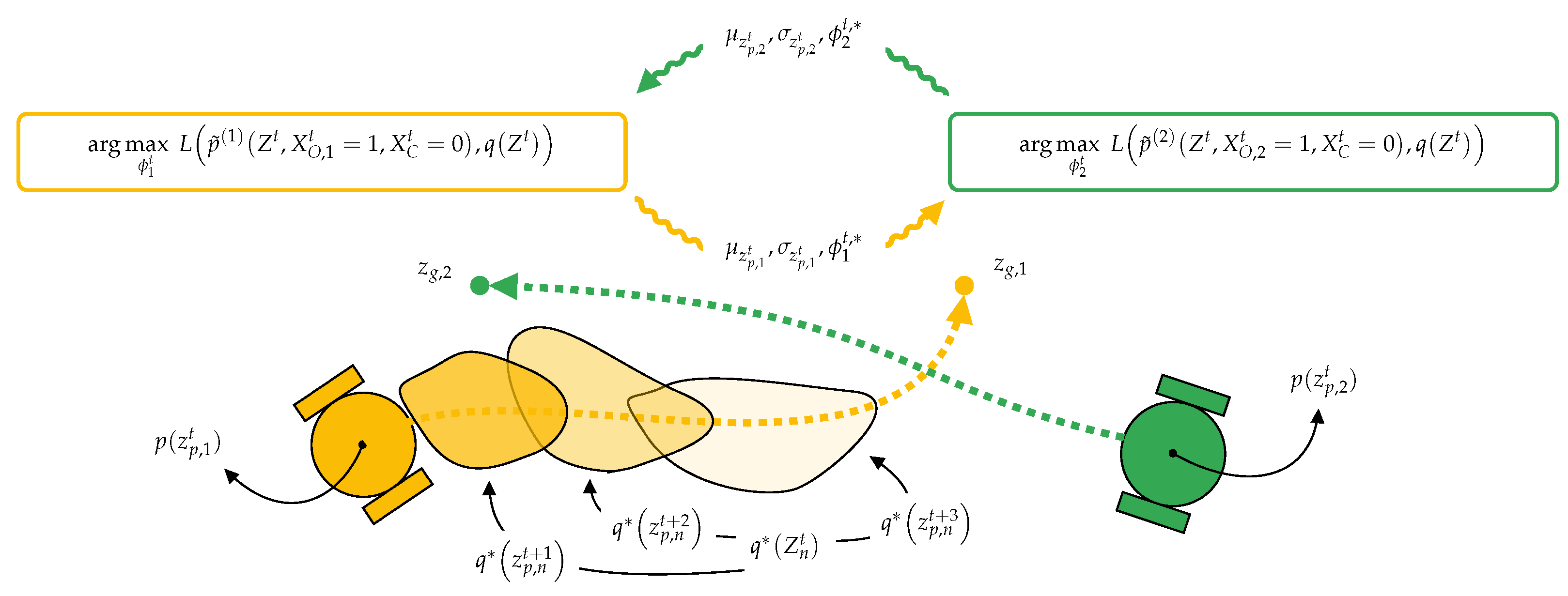
where ${\varphi }_n^t=\left\{\begin{array}{c}{\alpha }_n^t,{\beta }_n^t,\dots ,{\alpha }_n^{kt-1},{\beta }_n^{kt-1}\end{array}\right\}$, and broadcast the result ${\varphi }_n^{t,*}$ to the other vehicles as illustrated in Figure 2. In practice, to ease the computational burden, some of the terms can be removed from Equation (29), as only the evaluation of the constraints involving the n’th robot is non-constant. Overall we have divided the original approximation problem in Equation (21) into a series of less computationally demanding sub-problems that can be solved distributively by each of the robots. The next section presents a simulation study and a real world experiment utilizing this algorithm to make multiple robots safely navigate the same environment, and we will refer to it as “Stochastic Variational Message-passing for Multi-robot Navigation” (SVMMN).

4. Validation

To validate SVMMN described in Section 3, we performed both a simulation study and a real-world experiment, described in Section 4.1 and Section 4.2, respectively. In both cases, the models described in Section 3.1 were implemented utilizing the probabilistic programming language Pyro [14], and Pyro’s build-in stochastic variational inference solver was used. For solver options, we chose “Trace_ELBO”, thus implicitly using the Kullback–Leibler divergence, and the commonly used “Adam” stochastic optimization solver with 10 epochs/iterations per sent message.

4.1. Simulations

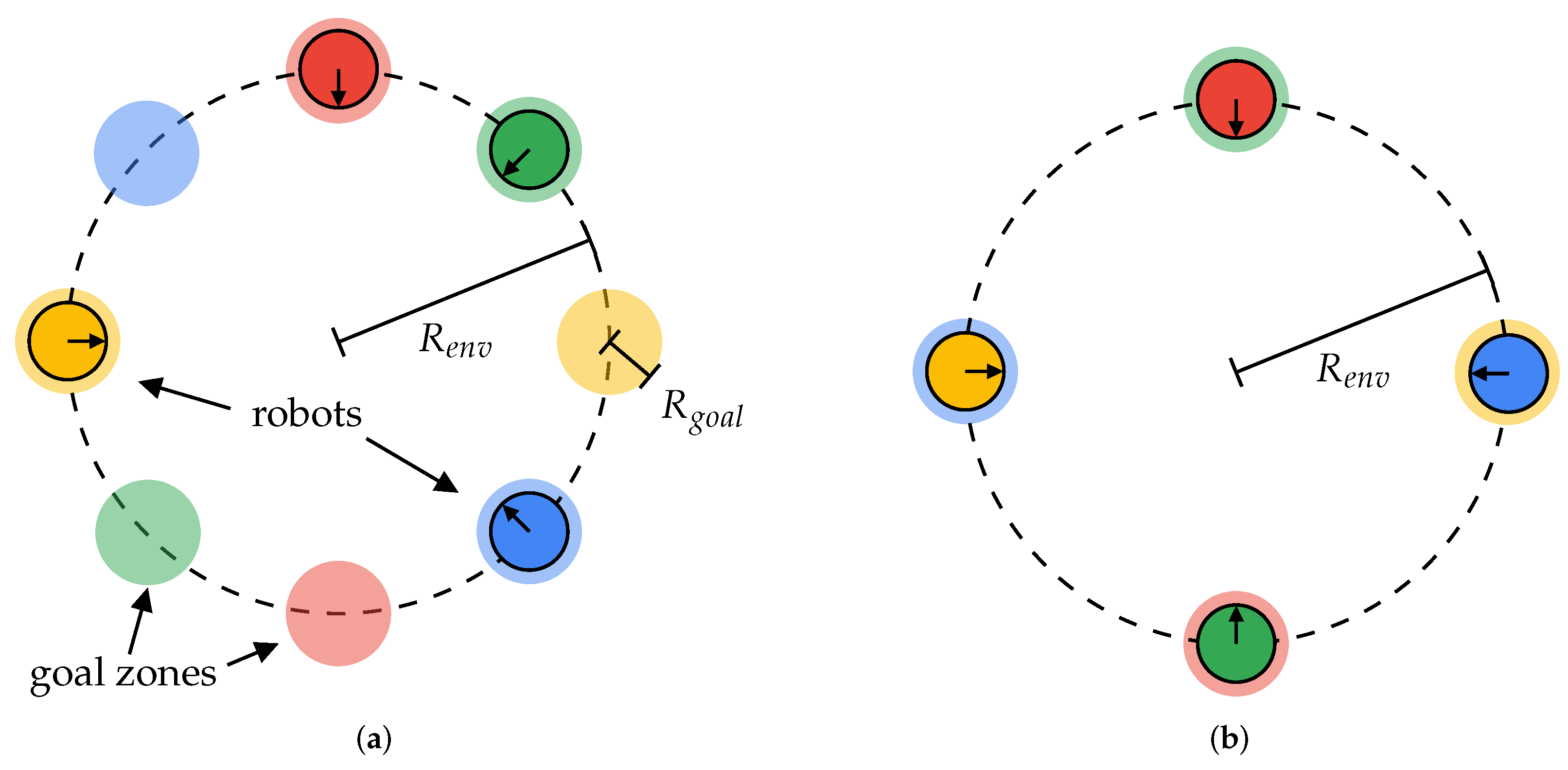
To evaluate the stochastic properties of SVMMN, we implemented a simple simulation environment for simulating N uni-cycle robots in parallel and in an asynchronous fashion. For ease of future comparison of algorithms, the environment was created according to the OpenAI Gym API [42]. Currently, the environment implements multiple scenarios commonly used to evaluate multi-robot collision avoidance algorithms: the antipodal goal circle scenario with both evenly distributed initialisation and with random initialisation used in, e.g., [29,32,34,37], and the antipodal circle swapping scenario used in, e.g., [27,28,29,30,31,32,33,34,35,38,39]. Both scenarios are illustrated in Figure 3. For each of the robots in these scenarios, two goal zones with a radius, $R_{goal}$, are generated evenly on the circumference of a circle with radius, $R_{env}$. When the simulation starts, each of the robots are initialized with a position in the centre of one of their respective goal zones. The goal of the robots is then to drive either one time or as many times as possible between the two goal zones without colliding with the robots during the simulated time. While both scenarios cause unnaturally crowded environments, the antipodal circle swapping scenario is specifically designed to provoke reciprocal dances [43] and deadlocks, whereas running the antipodal goal circle scenario with random initialisation for longer durations seems to cause more natural and diverse interactions. Results of simulations for both of these scenarios are summarized in the following sections. The environment, together with the code, data, and an accompanying video for each of the simulations, are available at [44].

Table A1. Parameters used during the simulations and the real-world experiment.

Parameter	General
$\underline{z_{a,n}^t}$, $\overline{z_{a,n}^t}$	$[-0.22,-2.84]$, $[0.22,2.84]$
M	$[0.05,0.05,0.10]$
$\Delta T$	1 s
k	4
$d_{min}$	$R_n+R_m$
	Real-world Experiment
	Robot 1	Robot 2
$R_n$	138 mm
$R_{goal}$	$0.2$ m
$z_{g,n}$	${[0.00,0.00]}^T$, ${[2.00,1.00]}^T$	${[0.50,0.13]}^T$, ${[1.50,1.87]}^T$
$c_1$, $c_2$	3, 25
	Antipodal Goal Circle
N	12
$R_n$	138 mm $\pm 20\%$
$R_{env},R_{goal}$	2 m, $0.25$ m
$c_1$, $c_2$	3, 5
${\sigma }_{z_{q,n}^t}$	$\mathrm{Diag}{\left(\frac{0.05\mathrm{m}}{3},\frac{0.05\mathrm{m}}{3},\frac{2.5^{\circ }}{3}\right)}^2$
	Antipodal Circle Swapping
N	$2,4,8,16,32$
$R_n$	200 mm
$R_{env},R_{goal}$	4 m, $0.1$ m
$c_1$, $c_2$	2, 5
${\sigma }_{z_{q,n}^t}$	$\mathrm{Diag}{\left(\frac{0.12\mathrm{m}}{3},\frac{0.12\mathrm{m}}{3},\frac{2.5^{\circ }}{3}\right)}^2$

in Appendix A summarizes the parameters chosen for the model, environment, and simulations. During the simulations, the real-time factor was adjusted to allow the robots to send approximately 3–4 messages per time-step, imitating the capabilities of the hardware used in the real world experiment.

4.1.1. The Antipodal Goal Circle Scenario

A series of 50 simulations of the antipodal goal circle scenario with 12 robots, and a simulated duration of 300 s were conducted. The simulations were performed with robots having physical properties similar to the robots used in the real world experiment. To quantify the ability of SVMMN to avoid collisions, we utilize the minimum separating distance (MSD) metric also used in [45]. We calculate the MSD of the i’th simulation as the minimum distance between any of the robots during the whole simulation:

$$\begin{array}{cc}\hfill \mathrm{MSD}\left(\mathrm{i}\right)& =\underset{t\in [0,300]}{min}SSD(t,i),\hfill \end{array}$$

where

$$\begin{array}{cc}\hfill SSD(t,i)& =\underset{\begin{array}{c}n\in [1,N-1]\hfill \\ m\in [n+1,N]\hfill \end{array}}{min}Dist\left(S_n^{t,i},S_m^{t,i}\right)=\underset{\begin{array}{c}n\in [1,N-1]\hfill \\ m\in [n+1,N]\hfill \end{array}}{min}\left|\right|z_{p,n}^{t,i}-z_{p,m}^{t,i}\left|\right|-R_n-R_m,\hfill \end{array}$$

(30)

$S_n^{t,i}$ is the geometrical set describing the shape and position of the n’th robots at time t, $z_{p,n}^{t,i}$ is the position of the n’th robot at time t in the i’th simulation, $R_n^i$ is the radius of the n’th robot, and the last equality in Equation (30) assumes that a disk can describe the robots. The MSD metric has the natural interpretation that a value strictly greater than 0 implies no collisions. Figure 4 shows the smallest separating distance (SSD) between any of the robots during all of the simulation, together with the mean of the MSD of the 50 simulations, and the smallest MSD recorded in any of the simulations. As seen from Figure 4, the MSD is strictly greater than 0 at any time, thus 0 collisions occurred. Figure 5 shows how many times the robots reached a goal zone during the simulations. These plots indicate that no deadlock occurred during the simulations. From these simulations, it can be concluded that SVMMN successfully manages to guide the robots towards their goals while still avoiding collisions.

4.1.2. The Antipodal Circle Swapping Scenario

A series of 10 simulations of the antipodal goal circle scenario with 4, 8, 16, and 32 robots were conducted. The simulations were stopped when all robots had reached their first goal. To make the results comparable with the B-UAVC algorithm [35], we adjusted the simulated radius of the robots together with the noise parameters to fit those used for simulations in [35]. Figure 6 presents the results of the simulation. As we do not use the same maximum velocities as in [35], we have normalized the travel distance and the travel time, with the minimum possible travel distance and time, respectively. As indicated by the MSD in Figure 6 zero collisions occurred during these simulations as well. Comparing SVMMN to B-UAVC, SVMMN generally seems to take a shorter path. For a small number of robots in the environment, B-UAVC has the smallest travel time despite SVMMN taking the shortest path. Data from the simulations reveal that the maximum translational velocity reference generated by SVMMN during the simulations with two robots was only 85.9% of the possible translational velocity. This is despite there being nothing to avoid most of the time, indicating that our approach generally picks velocities conservatively. This conservatism could be explained by the use of the Kullback–Leibler divergence, which tends to make the variational distribution, $q\left(z\right)$, cover a larger part of the true distribution, $p\left(z\right|x)$, rather then the most probable mode [13]. However, for a large number of robots, SVMMN still seems superior. Thus, from these simulations it can be concluded that SVMMN performs as well as, if not better than, B-UAVC specifically made for the problem of multi-robot collision avoidance.

4.2. Real-Wold Experiment

The real-wold experiment was performed with two TurtleBot3 Burger robots, each equipped with the standard lidar and an Intel NUC10FNK as the on-board processing unit. The parameters chosen for the model are summarized in Table A1 in Appendix A. To facilitate communication between the robots as needed for message-passing as described in Section 3.2, the meta operating system ROS2 was utilized. As the communication medium, 5 Ghz Wi-Fi provided by an Asus rt-ax92u router was used. As in the simulations, the robots were programmed to utilize alternating goal locations, $z_{g,n}$, each time they reached within 20cm of their current goal locations. To provide the estimate of the robots current pose distribution, $p\left(z_{q,n}^t\right)$, we utilized AMCL from the Nav2 ROS2 package [40]. The implemented algorithm is available at [46].

The results of the experiments are shown in Figure 7, Figure 8 and Figure 9. On average, the robots managed to solve their sub-problem and sent a solution to the other robot $3.01$ times per time-step. Figure 7 shows the full path taken by the robots during the 388 s long experiment. Robot 0 and Robot 1 travelled approximately $37.5$ m and $34.8$ m, respectively, while reaching their goals 17 times each giving plenty of opportunities for collisions.

Figure 8 shows the distance between the robots and their respective goal together with the SSD between the two robots themselves during the experiments, and the MSD for the whole test. In this test, the MSD was $7.8$ cm. From the plot, it is clear to see that the robots manage to reach their goal several times, while keeping a distance larger than $d_{min}$ from each other.

Figure 9 illustrates in more detail how SVMMN behaves in one of the situations where the robots were close to each other. To avoid a collision, at time $t=33$ robot 2 waits for robot 1 to pass. At the time $t=34$, robot 1 has passed and robot 2 begins planning a trajectory towards its goal and drives towards the goal at $t>34$. At time $t=39$, robot 1 has reached one of its goals and starts planning a trajectory towards its other goal. However, for $t>39$ robot 2 is blocking robots 1’s path, and therefore robot 1 does not drive that far.

Overall, the experiment illustrates how SVMMN successfully manages to make the robots drive to their goals while avoiding collisions despite the uncertainty in the localization from AMCL and uncertainty in the future movement of the other vehicle.

5. Conclusions

In this paper, we have discussed how variational inference can be a tractable way of solving robotics problems with non-neglectable uncertainties. More specifically, we have shown how two main solution approaches to variational inference, message-passing algorithms, and stochastic variational inference, relate. We outline how these two approaches can be potentially combined to flexibly solve problems with uncertainty in a distributed manner. By deriving and implementing an algorithm for navigation of multiple robots with cooperative avoidance under uncertainty, we furthermore demonstrate the feasibility of the proposed approach. Through simulations, we show that the derived algorithm works with multiple robots, and performs as well as, if not better than, the state of the art algorithm B-UAVC. Finally, we demonstrate that the derived algorithm works in a real-world experiment with two mobile robots.

6. Discussion

Many algorithms in robotics are already based on and derived directly from probabilistic models. The wide set of possible models that can be employed in stochastic variational inference should make it straightforward to apply the approach proposed in this paper to many of these probabilistic models, thereby resulting in new and interesting algorithms. Furthermore, due to the separation into sub-problems, the approach could potentially lead the way for offloading more computations to the cloud. As variational inference can incorporate neural networks, the approach also allows for the combination of classical modelling based methods and modern purely learning-based methods.

References

- Thrun, S.; Burgard, W.; Fox, D. Probabilistic Robotics. Intelligent Robotics and Autonomous Agents; MIT Press: Cambridge, MA, USA, 2005; pp. 1–647. [Google Scholar]
- Zhang, C.; Bütepage, J.; Kjellström, H.; Mandt, S. Advances in Variational Inference. IEEE Trans. Pattern Anal. Mach. Intell. 2019, 41, 2008–2026. [Google Scholar] [CrossRef] [PubMed] [Green Version]
- Kalman, R.E. A New Approach to Linear Filtering and Prediction Problems. Trans. ASME-Basic Eng. 1960, 82, 35–45. [Google Scholar] [CrossRef] [Green Version]
- Pfingsthorn, M.; Birk, A. Simultaneous localization and mapping with multimodal probability distributions. Int. J. Robot. Res. 2013, 32, 143–171. [Google Scholar] [CrossRef]
- Montemerlo, M.; Thrun, S.; Koller, D.; Wegbreit, B. FastSLAM: A Factored Solution to the Simultaneous Localization and Mapping Problem. In Proceedings of the Eighteenth National Conference on Artificial Intelligence, Edmonton, AB, Canada, 28 July–1 August 2002; American Association for Artificial Intelligence: Burgess Drive Menlo Park, CA, USA, 2002; pp. 593–598. [Google Scholar]
- Mirchev, A.; Kayalibay, B.; Soelch, M.; van der Smagt, P.; Bayer, J. Approximate Bayesian inference in spatial environments. arXiv 2019, arXiv:1805.07206. [Google Scholar]
- Fang, K.; Zhu, Y.; Garg, A.; Savarese, S.; Fei-Fei, L. Dynamics Learning with Cascaded Variational Inference for Multi-Step Manipulation. In Proceedings of the Conference on Robot Learning, Virtual, 16–18 November 2020; Kaelbling, L.P., Kragic, D., Sugiura, K., Eds.; PMLR: Reykjavik, Iceland, 2020; Volume 100, pp. 42–52. [Google Scholar]
- Shankar, T.; Gupta, A. Learning Robot Skills with Temporal Variational Inference. In Proceedings of the 37th International Conference on Machine Learning, Virtual, 13–18 July 2020; III, H.D., Singh, A., Eds.; PMLR: Reykjavik, Iceland, 2020; Volume 119, pp. 8624–8633. [Google Scholar]
- Pignat, E.; Lembono, T.; Calinon, S. Variational Inference with Mixture Model Approximation for Applications in Robotics. In Proceedings of the 2020 IEEE International Conference on Robotics and Automation (ICRA), Paris, France, 31 May–31 August 2020; pp. 3395–3401. [Google Scholar] [CrossRef]
- Mahajan, A.; Rashid, T.; Samvelyan, M.; Whiteson, S. MAVEN: Multi-Agent Variational Exploration. In Advances in Neural Information Processing Systems; Wallach, H., Larochelle, H., Beygelzimer, A., d’Alché-Buc, F., Fox, E., Garnett, R., Eds.; Curran Associates, Inc.: New York, NY, USA, 2019; Volume 32. [Google Scholar]
- Le, H.M.; Yue, Y.; Carr, P.; Lucey, P. Coordinated Multi-Agent Imitation Learning. In Proceedings of the 34th International Conference on Machine Learning, Sydney, Australia, 6–11 August 2017; Precup, D., Teh, Y.W., Eds.; Volume 70, pp. 1995–2003. [Google Scholar]
- Zhi, W.; Ott, L.; Senanayake, R.; Ramos, F. Continuous Occupancy Map Fusion with Fast Bayesian Hilbert Maps. In Proceedings of the 2019 International Conference on Robotics and Automation (ICRA), Montreal, QC, Canada, 20–24 May 2019; pp. 4111–4117. [Google Scholar] [CrossRef]
- Minka, T. Divergence Measures and Message Passing; Technical Report MSR-TR-2005-173; Microsoft: Redmond, Washington, USA, 2005. [Google Scholar]
- Bingham, E.; Chen, J.P.; Jankowiak, M.; Obermeyer, F.; Pradhan, N.; Karaletsos, T.; Singh, R.; Szerlip, P.A.; Horsfall, P.; Goodman, N.D. Pyro: Deep Universal Probabilistic Programming. J. Mach. Learn. Res. 2019, 20, 28:1–28:6. [Google Scholar]
- Krishnan, R.G.; Shalit, U.; Sontag, D. Structured Inference Networks for Nonlinear State Space Models. In Proceedings of the Thirty-First AAAI Conference on Artificial Intelligence, AAAI’17, San Francisco, CA, USA, 4–9 February 2017; AAAI Press: Palo Alto, CA, USA, 2017; pp. 2101–2109. [Google Scholar]
- Winn, J.; Bishop, C.M. Variational Message Passing. J. Mach. Learn. Res. 2005, 6, 661–694. [Google Scholar]
- Ranganath, R.; Gerrish, S.; Blei, D. Black Box Variational Inference. In Proceedings of the Seventeenth International Conference on Artificial Intelligence and Statistics, Reykjavic, Iceland, 22–25 April 2014; Kaski, S., Corander, J., Eds.; PMLR: Reykjavik, Iceland, 2014; Volume 33, pp. 814–822. [Google Scholar]
- Kucukelbir, A.; Tran, D.; Ranganath, R.; Gelman, A.; Blei, D.M. Automatic Differentiation Variational Inference. J. Mach. Learn. Res. 2017, 18, 1–45. [Google Scholar]
- Hoffman, M.D.; Blei, D.M.; Wang, C.; Paisley, J. Stochastic Variational Inference. J. Mach. Learn. Res. 2013, 14, 1303–1347. [Google Scholar]
- Li, Y.; Turner, R.E. Rényi Divergence Variational Inference. In Advances in Neural Information Processing Systems; Lee, D., Sugiyama, M., Luxburg, U., Guyon, I., Garnett, R., Eds.; Curran Associates, Inc.: New York, NY, USA, 2016; Volume 29. [Google Scholar]
- Wang, D.; Liu, H.; Liu, Q. Variational Inference with Tail-adaptive f-Divergence. In Advances in Neural Information Processing Systems; Bengio, S., Wallach, H., Larochelle, H., Grauman, K., Cesa-Bianchi, N., Garnett, R., Eds.; Curran Associates, Inc.: New York, NY, USA, 2018; Volume 31. [Google Scholar]
- Augugliaro, F.; Lupashin, S.; Hamer, M.; Male, C.; Hehn, M.; Mueller, M.W.; Willmann, J.S.; Gramazio, F.; Kohler, M.; D’Andrea, R. The Flight Assembled Architecture installation: Cooperative construction with flying machines. IEEE Control Syst. Mag. 2014, 34, 46–64. [Google Scholar] [CrossRef]
- Augugliaro, F.; Schoellig, A.P.; D’Andrea, R. Dance of the Flying Machines: Methods for Designing and Executing an Aerial Dance Choreography. IEEE Robot. Autom. Mag. 2013, 20, 96–104. [Google Scholar] [CrossRef]
- Queralta, J.P.; Taipalmaa, J.; Can Pullinen, B.; Sarker, V.K.; Nguyen Gia, T.; Tenhunen, H.; Gabbouj, M.; Raitoharju, J.; Westerlund, T. Collaborative Multi-Robot Search and Rescue: Planning, Coordination, Perception, and Active Vision. IEEE Access 2020, 8, 191617–191643. [Google Scholar] [CrossRef]
- Loke, S.W. Cooperative Automated Vehicles: A Review of Opportunities and Challenges in Socially Intelligent Vehicles Beyond Networking. IEEE Trans. Intell. Veh. 2019, 4, 509–518. [Google Scholar] [CrossRef]
- Fiorini, P.; Shiller, Z. Motion Planning in Dynamic Environments Using Velocity Obstacles. Int. J. Robot. Res. 1998, 17, 760–772. [Google Scholar] [CrossRef]
- Claes, D.; Hennes, D.; Tuyls, K.; Meeussen, W. Collision avoidance under bounded localization uncertainty. In Proceedings of the 2012 IEEE/RSJ International Conference on Intelligent Robots and Systems, Algarve, Portugal, 7–12 October 2012; pp. 1192–1198. [Google Scholar] [CrossRef]
- Alonso-Mora, J.; Rufli, M.; Siegwart, R.; Beardsley, P. Collision avoidance for multiple agents with joint utility maximization. In Proceedings of the 2013 IEEE International Conference on Robotics and Automation, Karlsruhe, Germany, 6–10 May 2013; pp. 2833–2838. [Google Scholar] [CrossRef] [Green Version]
- Snape, J.; van den Berg, J.; Guy, S.J.; Manocha, D. Smooth and collision-free navigation for multiple robots under differential-drive constraints. In Proceedings of the 2010 IEEE/RSJ International Conference on Intelligent Robots and Systems, Taipei, Taiwan, 18–22 October 2010; pp. 4584–4589. [Google Scholar] [CrossRef]
- Alonso-Mora, J.; Breitenmoser, A.; Rufli, M.; Beardsley, P.; Siegwart, R. Optimal Reciprocal Collision Avoidance for Multiple Non-Holonomic Robots. In Distributed Autonomous Robotic Systems: The 10th International Symposium; Martinoli, A., Mondada, F., Correll, N., Mermoud, G., Egerstedt, M., Hsieh, M.A., Parker, L.E., Støy, K., Eds.; Springer: Berlin/Heidelberg, Germany, 2013; pp. 203–216. [Google Scholar] [CrossRef] [Green Version]
- Rufli, M.; Alonso-Mora, J.; Siegwart, R. Reciprocal Collision Avoidance With Motion Continuity Constraints. IEEE Trans. Robot. 2013, 29, 899–912. [Google Scholar] [CrossRef]
- Bareiss, D.; van den Berg, J. Generalized reciprocal collision avoidance. Int. J. Robot. Res. 2015, 34, 1501–1514. [Google Scholar] [CrossRef]
- Alonso-Mora, J.; Beardsley, P.; Siegwart, R. Cooperative Collision Avoidance for Nonholonomic Robots. IEEE Trans. Robot. 2018, 34, 404–420. [Google Scholar] [CrossRef] [Green Version]
- Wang, L.; Ames, A.D.; Egerstedt, M. Safety Barrier Certificates for Collisions-Free Multirobot Systems. IEEE Trans. Robot. 2017, 33, 661–674. [Google Scholar] [CrossRef]
- Zhu, H.; Brito, B.; Alonso-Mora, J. Decentralized probabilistic multi-robot collision avoidance using buffered uncertainty-aware Voronoi cells. Auton. Robot. 2022, 46, 401–420. [Google Scholar] [CrossRef]
- Hoffmann, G.M.; Tomlin, C.J. Decentralized cooperative collision avoidance for acceleration constrained vehicles. In Proceedings of the 2008 47th IEEE Conference on Decision and Control, Cancun, Mexico, 9–11 December 2008; pp. 4357–4363. [Google Scholar] [CrossRef]
- Shahriari, M.; Biglarbegian, M. A Novel Predictive Safety Criteria for Robust Collision Avoidance of Autonomous Robots. IEEE/ASME Trans. Mechatron. 2021, 1–11. [Google Scholar] [CrossRef]
- Rodríguez-Seda, E.J.; Stipanović, D.M.; Spong, M.W. Guaranteed Collision Avoidance for Autonomous Systems with Acceleration Constraints and Sensing Uncertainties. J. Optim. Theory Appl. 2016, 168, 1014–1038. [Google Scholar] [CrossRef]
- Sivanathan, K.; Vinayagam, B.K.; Samak, T.; Samak, C. Decentralized Motion Planning for Multi-Robot Navigation using Deep Reinforcement Learning. In Proceedings of the 2020 3rd International Conference on Intelligent Sustainable Systems (ICISS), Thoothukudi, India, 3–5 December 2020; pp. 709–716. [Google Scholar] [CrossRef]
- Macenski, S.; Martin, F.; White, R.; Ginés Clavero, J. The Marathon 2: A Navigation System. In Proceedings of the 2020 IEEE/RSJ International Conference on Intelligent Robots and Systems (IROS), Las Vegas, NV, USA, 25–29 October 2020. [Google Scholar]
- Levine, S. Reinforcement Learning and Control as Probabilistic Inference: Tutorial and Review. arXiv 2018, arXiv:1805.00909. [Google Scholar]
- Brockman, G.; Cheung, V.; Pettersson, L.; Schneider, J.; Schulman, J.; Tang, J.; Zaremba, W. OpenAI Gym. arXiv 2016, arXiv:1606.01540. [Google Scholar]
- Johnson, J.K. The Colliding Reciprocal Dance Problem: A Mitigation Strategy with Application to Automotive Active Safety Systems. arXiv 2019, arXiv:1909.09224. [Google Scholar]
- Damgaard, M.R. Multi Robot Planning Simulation. 2022. Available online: https://github.com/damgaardmr/probMind/tree/d0ba27687b373ff04eb790ef38b21ca8572d8c8a/examples/multiRobotPlanning (accessed on 1 February 2022).
- Nishimura, H.; Mehr, N.; Gaidon, A.; Schwager, M. RAT iLQR: A Risk Auto-Tuning Controller to Optimally Account for Stochastic Model Mismatch. IEEE Robot. Autom. Lett. 2021, 6, 763–770. [Google Scholar] [CrossRef]
- Damgaard, M.R. Variational Inference Navigation. 2021. Available online: https://github.com/damgaardmr/VI_Nav/tree/8af532f5e6618d46f3498460af6459e57261fc91 (accessed on 1 February 2022).
Figure 1.
We propose to solve complicated robotics problems explicitly, taking uncertainty into account by utilising variational inference as seen in the single blue box. To distribute the necessary computations, we propose to utilise the concept of message-passing algorithms to divide the overall problem into a set of sub-problems that can potentially be sparsely connected, as illustrated in the green box with blue boxes inside. To make these sub-problems computationally tractable, we furthermore propose to solve them utilizing stochastic variational inference as seen in the green box with yellow boxes inside.
Figure 2.
The derived algorithm for cooperative navigation under uncertainty of multiple uni-cycle type robots works by letting each robot solve a sub-problem with stochastic variational inference and broadcast the solution to the other robots. Based on the broadcasted solution, a robot implicitly derives a distribution over the other robot’s future positions, , and uses the information in its sub-problem.
Figure 3.
Illustration of the simulated environment with . (a) Shows the antipodal goal circle scenario and (b) shows the antipodal circle swapping scenario. Two goal zones are generated for each of the robots, and the robot is initialized in the center of one of these goal zones.
Figure 4.
The smallest separating distance between any of the 12 robots during each of the 50 simulations.
Figure 5.
Histogram of the number of times the robots reached their goal zones during the simulations.
Figure 6.
Comparison of our algorithm called, “Stochastic Variational Message-passing for Multi-robot Navigation” (SVMMN), based on the combination of message-passing and stochastic variational inference, with B-UAVC [35] made specifically for the problem of multi-robot collision avoidance. The left, middle, and right plot shows the mean and standard deviations of the normalized travel distance (NTD), the normalized travel time (NTT), and the minimum separating distance (MSD) during the simulations, respectively. Notice that the data for B-UAVC are manually obtained from Figure 5 in [35].
Figure 7.
Traces of the two robots mean positions, , during the experiment, together with the mean of their initial positions distribution, , and goal areas defined as a circle with a radius of 20 cm around their goal locations, . The plots show how the robots sometimes deviate from the most direct path between their goal locations to avoid collision with each other.
Figure 8.
Each of the robots’ distances to their respective current goals, together with the distance between the two robots for the first 100 s of the experiment, and the minimum distance conservatively calculated as two times the length of the TurtleBot3 Burger platform, mm. The jumps in the plots of the robots’ distances to their goals are due to change in goal location. The plots show that the robots manage to reach their goal several times without violating a safe distance, , from each other.
Figure 9.
Kernel density estimate plots of the robots final predicted positions, , together with kernel density estimate plot of the robots initial positions, , the mean of the samples used to generate each plot, and , and finally the traces of their traversed paths, , for each . The plots clearly illustrate how the robots manage to negotiate trajectories that avoid a collision while taking the relevant uncertainties into account.
Publisher’s Note: MDPI stays neutral with regard to jurisdictional claims in published maps and institutional affiliations. |
© 2022 by the authors. Licensee MDPI, Basel, Switzerland. This article is an open access article distributed under the terms and conditions of the Creative Commons Attribution (CC BY) license (https://creativecommons.org/licenses/by/4.0/).
Share and Cite
MDPI and ACS Style
Damgaard, M.R.; Pedersen, R.; Bak, T. Study of Variational Inference for Flexible Distributed Probabilistic Robotics. Robotics 2022, 11, 38. https://0-doi-org.brum.beds.ac.uk/10.3390/robotics11020038
AMA Style
Damgaard MR, Pedersen R, Bak T. Study of Variational Inference for Flexible Distributed Probabilistic Robotics. Robotics. 2022; 11(2):38. https://0-doi-org.brum.beds.ac.uk/10.3390/robotics11020038
Chicago/Turabian StyleDamgaard, Malte Rørmose, Rasmus Pedersen, and Thomas Bak. 2022. "Study of Variational Inference for Flexible Distributed Probabilistic Robotics" Robotics 11, no. 2: 38. https://0-doi-org.brum.beds.ac.uk/10.3390/robotics11020038
Note that from the first issue of 2016, this journal uses article numbers instead of page numbers. See further details here.