Non-Linear Lumped-Parameter Modeling of Planar Multi-Link Manipulators with Highly Flexible Arms

Abstract

The problem of the trajectory-tracking and vibration control of highly flexible planar multi-links robot arms is investigated. We discretize the links according to the Hencky bar-chain model, which is an application of the lumped parameters techniques. In this approach, each link is considered as a kinematic chain of rigid bodies, and suitable springs are added in order to model bending resistance. The control strategy employed is based on an optimal input pre-shaping and a feedback of the joint angles to treat the effects of undesired disturbances. Some numerical examples are given to show the potentialities of the proposed control, and a comparison with a standard collocated Proportional-Derivative (PD) control strategy is performed. In particular, we study the cases of a linear and a parabolic trajectory with a polynomial time law chosen to minimize the onset of possible vibrations.

1. Introduction

Although the literature on flexible robotic manipulators is very varied and covers different aspects of the dynamic analysis and control of these mechanical systems [1,2,3,4,5,6], in industrial practice, the robotic arms are still treated as rigid multi-body systems. Only in aerospace, for evident weight issues, this strong assumption has long since been removed. In this context, however, moderately flexible links are considered to simplify the analysis and synthesis of rest-to-rest motion, trajectory-tracking and vibration control, resulting in a degradation of performance.

In this paper, we want to address the problem of considering planar multi-link highly flexible robotic arms whose transversal deflections are very large, and therefore, no linearization procedure is adoptable (refer to [7,8] for some relevant real applications). For these systems, it is possible to model the links with the continuous non-linear beam model of Euler–Bernoulli, i.e., the elastica theory [9,10,11,12,13,14,15]. However, as this continuous one-dimensional model is characterized by infinite degrees of freedom, it is rather difficult to analyze the manipulator’s motion and to design the related control. For this reason, usually a spatial discretization of the continuous model is resorted to. Typically, three methods of discretization are used: the assumed modes technique; the Finite Element Method (FEM); and the lumped parameters method. The assumed modes approach is an intrinsically linear method, and therefore, it is applicable only to a one-link system with small flexibility or multi-link systems in which the task time is much greater than the characteristic period of oscillation of the first modes. The latter assumption is strongly requested because a progressive linearization must be carried out in the neighborhood of the generic current configuration, which indeed varies with the motion [16,17]. The finite element method can be seen as a special case of the assumed modes technique, but it can be generalized to the nonlinear case and can therefore cover also the cases taken into account for the present study. As an example, we mention Du et al. [18], who address the problem of a non-linear 3D flexible manipulator with FE analysis. The discretization by lumped parameters [19,20] is one of the earliest methods and is characterized by an extreme simplicity of modeling and computational advantages. Moreover, being intrinsically nonlinear, it does not introduce any approximation due to some kind of linearization [21,22]. Although the finite element method converges faster than that of lumped parameters and requires a lower number of degrees of freedom to obtain the same accuracy, to deal with nonlinear cases, it is necessary to make use of a specific, rather complex formulation, which could be familiar to experts of computational mechanics, but less accessible to a larger audience (see, e.g., [23]). It should be noted, indeed, that the commercial FEM codes are rather lacking in dealing with the problem of large deflections of beams, to the best of the authors’ knowledge. There are many papers that analyze the accuracy of the lumped parameters approach from different points of view, and in all of them, it is possible to find that the error in the approximation with such a method is inversely proportional at least to the first power of the number of elements used [24,25]. In the case of a cantilever beam subject to flexural oscillations, the inverse square law for the error can be verified without difficulty [26]. This means that with a rather simple modeling method, it is possible to reach the desired degree of accuracy simply by appropriately selecting the number of elements; a thumb rule is to use 13 elements per wave-length to be analyzed [26]. In the past, often the lumped-parameter approach was underestimated because assigning spring lumped constants was considered not straightforward [3]. Unfortunately, this is the result of a certain compartmentalization of expertise that sometimes occurs [27]. Indeed, it is widely known to those dealing with beam homogenization how to properly assign these discretized constants of stiffness [28,29,30,31,32,33].

In this paper, we will use the lumped parameters approach because of its simplicity and versatility. In this formulation, an elastic rod is discretized into a set of rigid segments, which are free to rotate relative to their adjacent neighbors. Springs located in these joints give the system the ability to resist bending. The case study can be classified as an under-actuated system. Indeed, the considered multi-link arm is subject to a lower number of actuators than degrees of freedom. The particular formulation adopted, among the various advantages, could make use of widely established results in classical robotics for this type of problem since in fact the model adopted is a kinematic chain of rigid bodies (see, e.g., [34,35,36] and the references therein).

System flexibility leads to vibration and, in turn, to an imprecise positioning due mainly to a non-minimum phase character of the system. As an illustrative numerical example, we consider a control strategy for the problem of the trajectory-tracking in the framework of the input shaping control [37,38,39] with a feedback for the stabilization of the response. In particular, to obtain the command torques, instead of using proper filtering as is usually done, we formulate an optimal control problem with the aim of minimizing the positioning error of the tip manipulator (see, e.g., [40]). This variational approach has been adopted for trajectory planning both for flexible [41,42] and for rigid arms [6]. Herein, instead of obtaining a trajectory with the desired mechanical characteristics, the best possible input command is found to follow a given trajectory.

The paper is organized as follows: Section 2 is devoted to describing the adopted discrete method, which is applied to a planar two-link flexible arm. Section 3 reports on numerical simulations for some trajectory-tracking cases and a comparison with a standard control approach. The paper ends with the conclusions and some future perspectives.

2. Dynamic Modeling of the Flexible Robot Manipulator

To address the complex problem of trajectory control of the tip for flexible robot manipulators, we propose to study an elemental prototype case whose behavior is rich enough to easily extend the obtained results to more generalized situations, namely more links or manipulators subject to a 3D motion (see, e.g., [43] for the analogous 3D formulation). Specifically, a planar horizontal robot manipulator constituted of two highly flexible links is considered. Each link of the manipulator is characterized by a length ${\ell }_i$ (with $i=\{1,2\}$), a uniform distribution of stiffness and mass density and is driven by an actuator, with mass $m_{hi}$, inertia $J_{hi}$ and supplying a torque ${\tau }_i$. The manipulator eventually may carry a tip payload of mass $m_p$ and inertia $J_p$.

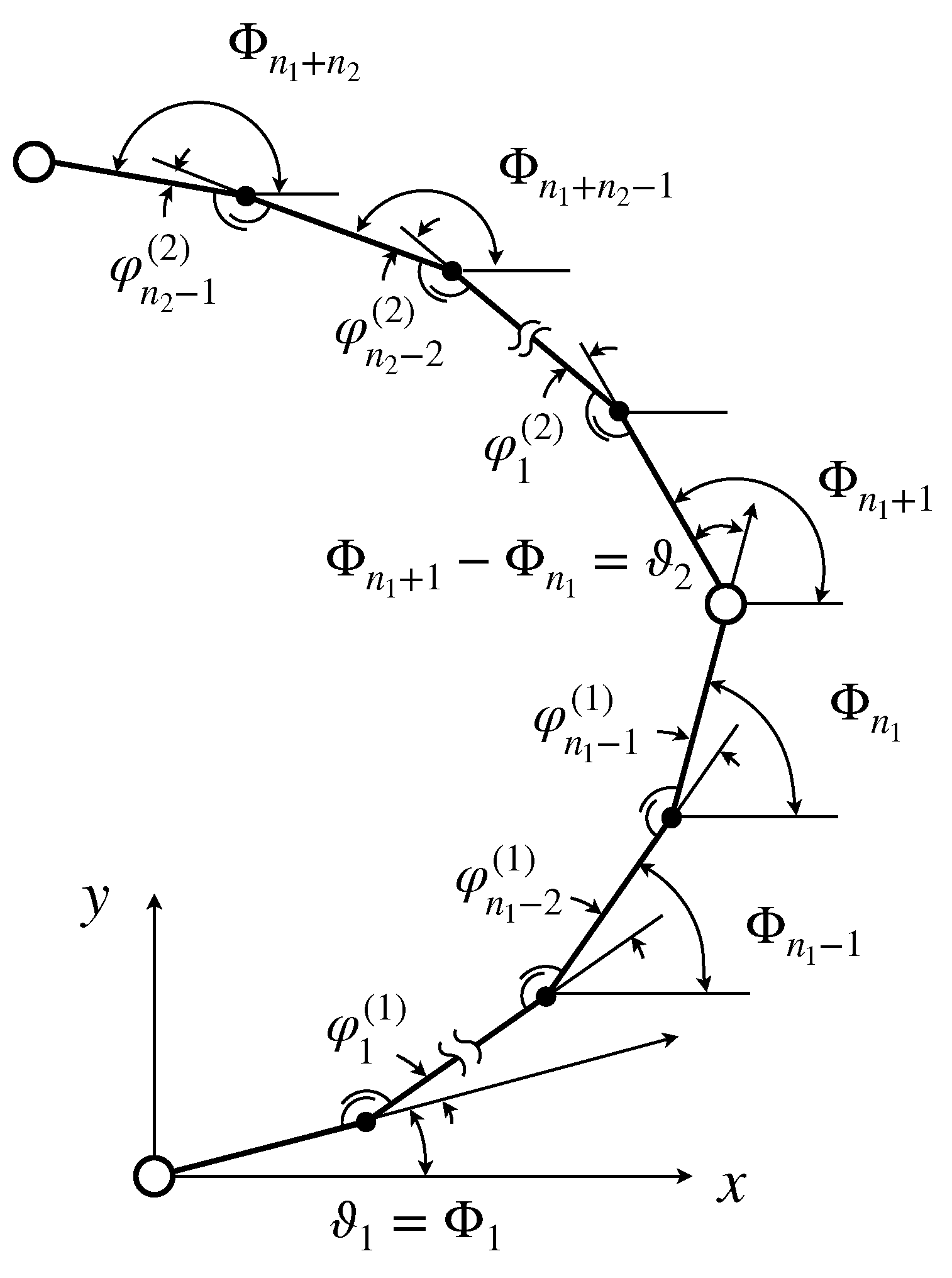
To model this system, we consider a lumped-parameter discretization. Since the manipulator is made up of two links, which can be modeled in the range of large deflections by the elastica theory, we adopt the well-known Hencky technique [28,29,43,44,45] to discretize the system and, then, using a more comfortable Lagrangian mechanical system, to study the motion of the robot and to design the trajectory tracing. Therefore, the considered discrete system consists of two articulated chains of $n_i$ rigid rods of length $\eta$ connected to each other by means of zero-torque hinges, also known as ‘pseudo-joints’. At each joint of the same link, a rotational spring is placed in order to model the resistance to being bent of the arm (see Figure 1). In other words, the torques provided by these springs represent the spatial discretization of the internal actions of the links, namely the bending moment. The Lagrangian coordinates, which describe the configurations of the manipulator are ${\mathsf{\Phi }}_j\left(t\right)$ (with $j=\{1,2,\dots n_1+n_2\}$). In particular, they represent the orientation of the rigid rods with respect to the x-axis. Moreover, the following definitions are useful to specify the angles of the actuation:

$$\left\{\begin{array}{c}{\vartheta }_1={\mathsf{\Phi }}_1\hfill \\ {\vartheta }_2={\mathsf{\Phi }}_{n_1+1}-{\mathsf{\Phi }}_{n_1}\hfill \end{array}\right.$$

(1)

for the two links, and the relative angles:

$$\left\{\begin{array}{cc}{\phi }_{h-1}^{\left(1\right)}={\mathsf{\Phi }}_h-{\mathsf{\Phi }}_{h-1}\hfill & \mathrm{with}h=2,\dots n_1\hfill \\ {\phi }_{k-1-n_1}^{\left(2\right)}={\mathsf{\Phi }}_k-{\mathsf{\Phi }}_{k-1}\hfill & \mathrm{with}k=n_1+2,\dots n_1+n_2\hfill \end{array}\right.$$

(2)

which are relevant to define the deformation energy of the links whose label is reported between parentheses as a superscript. Indeed, the relative angles can be used to describe a discrete point-wise curvature. The two links prior to deformation are straight. Their mass is discretized with lumped masses $m_i$ at the boundaries of each rigid segment by dividing the mass of each segment at its ends. The position of each point mass can be written as:

$$\left\{\begin{array}{c}{x}_j\left(t\right)=\sum _{k=1}^j\eta cos\left({\mathsf{\Phi }}_k\right)\hfill \\ y_j\left(t\right)=\sum _{k=1}^j\eta sin\left({\mathsf{\Phi }}_k\right)\hfill \end{array}\right.$$

(3)

and by a differentiation with respect to time, the velocities of the point masses are given by:

$$\left\{\begin{array}{c}{\dot{x}}_j\left(t\right)=-\sum _{k=1}^j\eta {\dot{\mathsf{\Phi }}}_{k}sin\left({\mathsf{\Phi }}_k\right)\hfill \\ {\dot{y}}_j\left(t\right)=\sum _{k=1}^j\eta {\dot{\mathsf{\Phi }}}_{k}cos\left({\mathsf{\Phi }}_k\right)\hfill \end{array}\right.$$

(4)

The equations of the motion can be derived from the Lagrangian:

$$\mathcal{L}=\mathfrak{K}-\mathsf{\Psi }$$

(5)

where $\mathfrak{K}$ and $\mathsf{\Psi }$ are the kinetic and potential energies of the system, respectively. Particularly, the kinetic energy can be obtained by the sum of three contributions, i.e., a term due to the links:

$${\mathfrak{K}}_{\ell }=\sum _{j=1}^{n_1+n_2}\frac{1}{2}{m}_j\left\{{\left[\sum _{k=1}^j\eta {\dot{\mathsf{\Phi }}}_{k}sin\left({\mathsf{\Phi }}_k\right)\right]}^2+{\left[\sum _{k=1}^j\eta {\dot{\mathsf{\Phi }}}_{k}cos\left({\mathsf{\Phi }}_k\right)\right]}^2\right\}$$

(6)

a term due to the two actuators:

$${\mathfrak{K}}_h=\frac{1}{2}{J}_{h1}{\dot{\mathsf{\Phi }}}_1^2+\frac{1}{2}{m}_{h2}\left({\dot{x}}_{n_1}^2+{\dot{y}}_{n_1}^2\right)+\frac{1}{2}{J}_{h2}{\dot{\mathsf{\Phi }}}_{n_1+1}^2$$

(7)

and the last term for the payload:

$${\mathfrak{K}}_p=\frac{1}{2}{m}_p\left({\dot{x}}_{n_1+n_2}^2+{\dot{y}}_{n_1+n_2}^2\right)+\frac{1}{2}{J}_p{\dot{\mathsf{\Phi }}}_{n_1+n_2}^2$$

(8)

The elastic potential energy $\mathsf{\Psi }$ is assumed to be:

$$\mathsf{\Psi }=\sum _{i=1}^2\sum _{j=1}^{n_i-1}{\kappa }_{bj}^{\left(i\right)}[1-cos({\phi }_j^{\left(i\right)})]$$

(9)

where a lumped bending stiffness ${\kappa }_{bj}^{\left(i\right)}=Y{J}_{{\ell }_i}/\eta$ associated with the rotational springs is introduced using the elastic modulus of the beam’s material, Y, and the second moment of the area of the beam’s cross-section, $J_{{\ell }_i}$ [46,47]. Note that the potential energy in Equation (9) is positive definite, and in the continuum limit, i.e., for $\eta$ tending to zero, the expression (9) becomes an energy density, which is quadratic in the curvature of the beam axis [46], in accord with the elastica theory. As a first approximation, we also consider a viscous dissipation (see, e.g., [48,49]), introducing the Rayleigh dissipation function:

$$\mathfrak{R}=\sum _{i=1}^2\sum _{j=1}^{n_i-1}\frac{1}{2}{c}_{bj}^{\left(i\right)}{\left({\dot{\phi }}_j^{\left(i\right)}\right)}^2$$

(10)

$c_{bj}^{\left(i\right)}$ being a lumped viscous coefficient. This type of dissipation can be associated with the rate of the bending deformation; thus with similar reasoning used for the elastic bending mode deformation, it is possible to evaluate the lumped dissipation with the expression: $c_{bj}^{\left(i\right)}=C_v{J}_{{\ell }_i}/\eta$, where the material parameter $C_v$ is the viscous coefficient of the beam material, which can be experimentally identified (see, e.g., [50]).

The Euler–Lagrange equations of motion, thus, are:

$$\frac{\partial }{\partial t}\left(\frac{\partial \mathfrak{K}}{\partial {\dot{\mathsf{\Phi }}}_i}\right)-\frac{\partial \mathfrak{K}}{\partial {\mathsf{\Phi }}_i}+\frac{\partial \mathsf{\Psi }}{\partial {\mathsf{\Phi }}_i}+\frac{\partial \mathfrak{R}}{\partial {\dot{\mathsf{\Phi }}}_i}=Q_i\mathrm{for}i=1\dots n_1+n_2$$

(11)

The virtual work of the torques applied by actuators at the basis of each link is:

$$\delta W={\tau }_1\delta {\vartheta }_1+{\tau }_2\delta {\vartheta }_2={\tau }_1\delta {\mathsf{\Phi }}_1+{\tau }_2\left(\delta {\mathsf{\Phi }}_{n_1+1}-\delta {\mathsf{\Phi }}_{n_1}\right)$$

(12)

hence, the only generalized forces different from zero are:

$$Q_1={\tau }_1,Q_{n_1+1}={\tau }_2,Q_{n_1}=-{\tau }_2$$

(13)

One of the performance specifications in a control system should be a satisfactory regulation against disturbances. Here, to test the effectiveness of the proposed control, we take into consideration two kinds of disturbances, due to the actual realization of the actuators, that add up to the torques introduced in Equation (13); specifically, friction torques, which arise at the actuated joints, and cogging torques, typical for electrical motors. The former disturbance is described by a Lund–Grenoble model [51], which is able to capture most of the major nonlinear effects involved in the considered case such as pre-sliding displacement, stick-slip motion, the Stribeck effect, and so forth; the latter disturbance, due to the interaction between the permanent magnets of the rotor and the slots of the stator, is modeled by means of a constitutive relationship, experimentally identified, i.e., a periodic function of the relative position between the stator and the rotor of the motor [52]. An evolution rule for the friction torques ${\tau }_{fi}$ is assumed as follows:

$$\frac{\mathrm{d}{\tau }_{fi}}{\mathrm{d}t}=k_i{\dot{\vartheta }}_i\left(1-\frac{{\tau }_{fi}}{{\tau }_L\left({\dot{\vartheta }}_i\right)}\mathrm{sign}\left({\dot{\vartheta }}_i\right)\right)$$

(14)

where ${\tau }_L({\dot{\vartheta }}_i)={\tau }_C+({\tau }_S-{\tau }_C)exp\left[-{\left({\dot{\vartheta }}_i/{\nu }_s\right)}^2\right]$ is the limit torque introduced to take into account the Stribeck effect. In detail, ${\tau }_S=0.2$ Nm is the static friction; ${\tau }_C=0.1$ Nm is the Coulomb friction torque; and ${\nu }_s=0.1$ s${}^{-1}$ represents the Stribeck velocity. The cogging torques are evaluated as a function of the angles ${\vartheta }_i$ as follows:

$${\tau }_{cgi}=T_{cg}\sum _{k=1}^6{B}_{k}sin\left(n_{p}k{\vartheta }_i\right)$$

(15)

where $T_{cg}=0.1$ Nm is the amplitude of the torque, $n_p=2$ is the number of poles of the motors and the coefficients of the trigonometric polynomial $B_k$ are assumed to be $\{-0.7937,-0.3586,-0.0341,0.0039,-0.0016,-0.0064\}$ in the performed simulations.

3. Numerical Examples for Some Trajectory-Tracking Cases

In this section, a control scheme for trajectory-tracking and vibration control of flexible arms is used to show the potentialities of the proposed formulation. This approach is based on an optimal design of the command torques applied to the actuated joints that aim at following the desired trajectory and reducing vibrations. The control strategy, thus, includes a feedforward control based on such a command input and a feedback control that stabilizes the $2R$ flexible robot along the desired trajectory by a joint-based collocated Proportional-Derivative (PD) controller [39]. Precisely, the optimal control technique is used to produce input profiles for the torques acting on the flexible system as described below. Since the command shaping technique does not require additional sensors or actuators, this technique is particular attractive in order to have a hardware apparatus for the control characterized by minimal equipment.

As a first step, we plan a desired trajectory ${\mathit{x}}_d\left(t\right)$ connecting the ends of each link from arbitrary initial points to desired final points in a given time interval $\mathcal{I}=[0,t_f]$, i.e., we set ${\mathit{x}}_d\left(t\right)=(x_{n_1,d},y_{n_1,d},x_{n_1+n_2,d},y_{n_1+n_2,d})$. Then, denoting the actual trajectory of the ends of each link, evaluated on the solution of Equation (11) in $\mathcal{I}$ without disturbances, with $\tilde{\mathit{x}}\left(t\right)=({\tilde{x}}_{n_1},{\tilde{y}}_{n_1},{\tilde{x}}_{n_1+n_2},{\tilde{y}}_{n_1+n_2})$, the optimal control problem for the design of the input torques can be formulated as follows:

Find the torques $\mathit{\tau }\left(t\right)=({\tau }_1,{\tau }_2)$ as real-valued smooth functions defined on $\mathcal{I}$, which minimize the continuous-time cost functional:

$$J(\tilde{\mathsf{\Phi }},\mathit{\tau },t)=\frac{1}{2}{\int }_0^{t_f}{(\tilde{\mathit{x}}-{\mathit{x}}_d)}^{\top }\mathit{R}(\tilde{\mathit{x}}-{\mathit{x}}_d)\mathrm{d}t$$

(16)

subject to the dynamic constraints that $\tilde{\mathit{x}}\left(t\right)$ is computed on the solution of Equation (11) with given initial conditions. $\mathit{R}$ is a constant diagonal positive definite weight matrix.

In detail, we directly minimize the functional J varying the torques ${\tau }_1\left(t\right)$ and ${\tau }_2\left(t\right)$ instead of solving the Euler–Lagrange equations, which may laboriously be obtainable by means of calculus of variations. Therefore, representing the torques ${\tau }_i$ in a discrete way as follows:

$${\overline{\tau }}_i\left(t\right)={\tau }_{0i}\left(t\right)+w\left(t\right)\sum _{h=0}^{n_d}{a}_h^{\left(i\right)}{p}_h\left(t\right)$$

(17)

where ${\tau }_{0i}\left(t\right)$ is a reference torque, $p_h\left(t\right)$ are interpolation functions defined on $\mathcal{I}$ and $w\left(t\right)$ is a proper window function, the problem (16) results in finding the coefficients $a_h^{\left(i\right)}$ that minimize the functional J evaluated with the approximated shapes ${\overline{\tau }}_i\left(t\right)$. The particular form chosen for Equation (17) is based on the idea of finding an approximate solution for the considered problem, by starting from the exact solution of a related, simpler problem and then adding a correction. The first term ${\tau }_{0i}\left(t\right)$, indeed, is the required torque evaluated for the 2R rigid robot, while the other term represents the correction needed to solve the primary problem. In particular, the function $w\left(t\right)$ is conceived of in order to account for a correction of the torques, which tends to zero at the beginning and at the end of the interval $\mathcal{I}$. In this way, a jump in the torques, responsible for the onset of possible vibrations, can be avoided. A possible choice of this function $w\left(t\right)$ is the Welch window, defined as:

$$w\left(t\right)=\left\{\begin{array}{cc}4\frac{t}{t_f}\left(1-\frac{t}{t_f}\right)\hfill & \mathrm{for}t\in \mathcal{I}\hfill \\ 0\hfill & \mathrm{outside}\mathcal{I}\hfill \end{array}\right.$$

(18)

Indeed, this window is designed, as many others, to moderate the sudden changes of a rectangular window and, thus, to improve dynamic range. Regarding the $p_h$ functions, thinking of a Taylor expansion properly truncated to express the torque corrections, we consider $p_h\left(t\right)=t^h$. Of course, the corrections can be expressed in alternative ways, for example a truncated Fourier series can also be a valid representation. In both cases, a convergence analysis is needed to determine how many terms should be taken into account to minimize the truncation error.

Once the optimal torques ${\tau }_{id}\left(t\right)$ are obtained by solving the problem (16), the complete control strategy can be expressed in the following way:

$${\tau }_i={\tau }_{di}+K_{Pi}({\vartheta }_{di}-{\vartheta }_i)+K_{Di}({\dot{\vartheta }}_{di}-{\dot{\vartheta }}_i)$$

(19)

where $({\vartheta }_i,{\dot{\vartheta }}_i)$ are related to the actual trajectory for the joint angles, directly measured by the motor encoders, while $({\vartheta }_{di},{\dot{\vartheta }}_{di})$ correspond to the desired trajectory, which is computed off-line by a numerical simulation of the manipulator performed using the optimal torques ${\tau }_{di}\left(t\right)$ as input. To choose the PD gains, a standard technique can be employed based on setting the natural frequencies, which govern the speed of response, as well as taking into account the saturation of each actuator (for a detailed description see, e.g., [53]).

To illustrate the potentialities of the proposed control strategy, we examine some representative examples in which the manipulator tip is constrained to move along two different paths, namely a straight line segment and a piece of parabolic curve.

In the first case, the desired coordinates for the end effector are assumed to be:

$$\left\{\begin{array}{c}{x}_{n_1+n_2,d}\left(t\right)={\ell }_1+{\ell }_2-s\left(t\right)cos\left(arctan\left(\frac{{\ell }_1}{{\ell }_1+{\ell }_2}\right)\right)\hfill \\ y_{n_1+n_2,d}\left(t\right)=s\left(t\right)sin\left(arctan\left(\frac{{\ell }_1}{{\ell }_1+{\ell }_2}\right)\right)\hfill \end{array}\right.$$

(20)

in which the time function $s\left(t\right)$ is a Peisekah polydyne, which is expressed as follows:

$$s\left(t\right)=A_d\left[126{\left(\frac{t}{t_f}\right)}^5-420{\left(\frac{t}{t_f}\right)}^6+540{\left(\frac{t}{t_f}\right)}^7-315{\left(\frac{t}{t_f}\right)}^8+70{\left(\frac{t}{t_f}\right)}^9\right]$$

(21)

where $A_d=\sqrt{{\ell }_1^2+{({\ell }_1+{\ell }_2)}^2}$ and the task time is set to $t_f=1$ s. The well-known time law (21) is chosen because the values of its derivatives with respect to time up to fourth order at the initial and final times are all zero. This feature is particularly desired to avoid exciting vibrations. Here, the initial configuration provides the robotic arm arranged along the x axis completely unfolded, while the final arrangement of the arm is characterized by having the end effector in the position of coordinates $(0,{\ell }_1)$.

In the second case, the desired coordinates for the tip manipulator follow the parabola:

$$\left\{\begin{array}{c}{x}_{n_1+n_2,d}\left(t\right)=\left({\ell }_1+{\ell }_2\right)-s\left(t\right)\left({\ell }_1+{\ell }_2\right)\hfill \\ y_{n_1+n_2,d}\left(t\right)={\ell }_{1}s{\left(t\right)}^2\hfill \end{array}\right.$$

(22)

where the function $s\left(t\right)$ is given by Equation (21) with $A_d=1$ and $t_f=1.25$ s. The initial and final configurations are set up as in the previous case.

In all the cases, we extend the desired time interval for a while in order to stabilize, in the optimization stage, the solution at the final configuration. The desired coordinates of the intermediate joint, $(x_{n_1,d},y_{n_1,d})$, have been calculated considering the robotic arm as a 2R rigid robot for both cases addressed.

Equations (11) are numerically solved by means of the computing system Simulink considering a 2R flexible arm with links of length ${\ell }_1={\ell }_2=0.5$ m and having a rectangular cross-section of size $50\times 2$ mm with a second moment of area $J_{{\ell }_1}=J_{{\ell }_2}=3.33\times {10}^{-11}$ m${}^4$. The links are discretized using 99 rigid segments. The Young modulus of the links is $Y=200$ GPa, and the mass of each of them is 0.3925 kg. The viscous coefficients are assumed to be $c_b^{\left(1\right)}=c_b^{\left(2\right)}=0.15$ Nms. The actuators are characterized by masses $m_{h1}=m_{h2}=1$ kg and moments of inertia $J_{h1}=J_{h2}=0.1$ kg m${}^2$, while the payload has $m_p=0.1$ kg and $J_p=0.005$ kg m${}^2$. For the implementation of the optimal problem, we assume the non-vanishing elements of $\mathit{R}$ to be $R_{11}=R_{22}=10$ and $R_{33}=R_{44}=100$ to give more importance to the tip error.

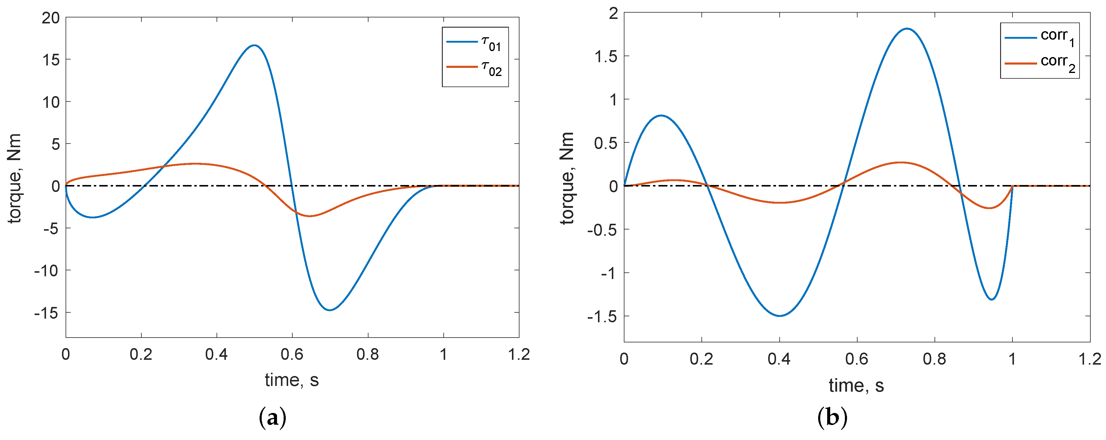
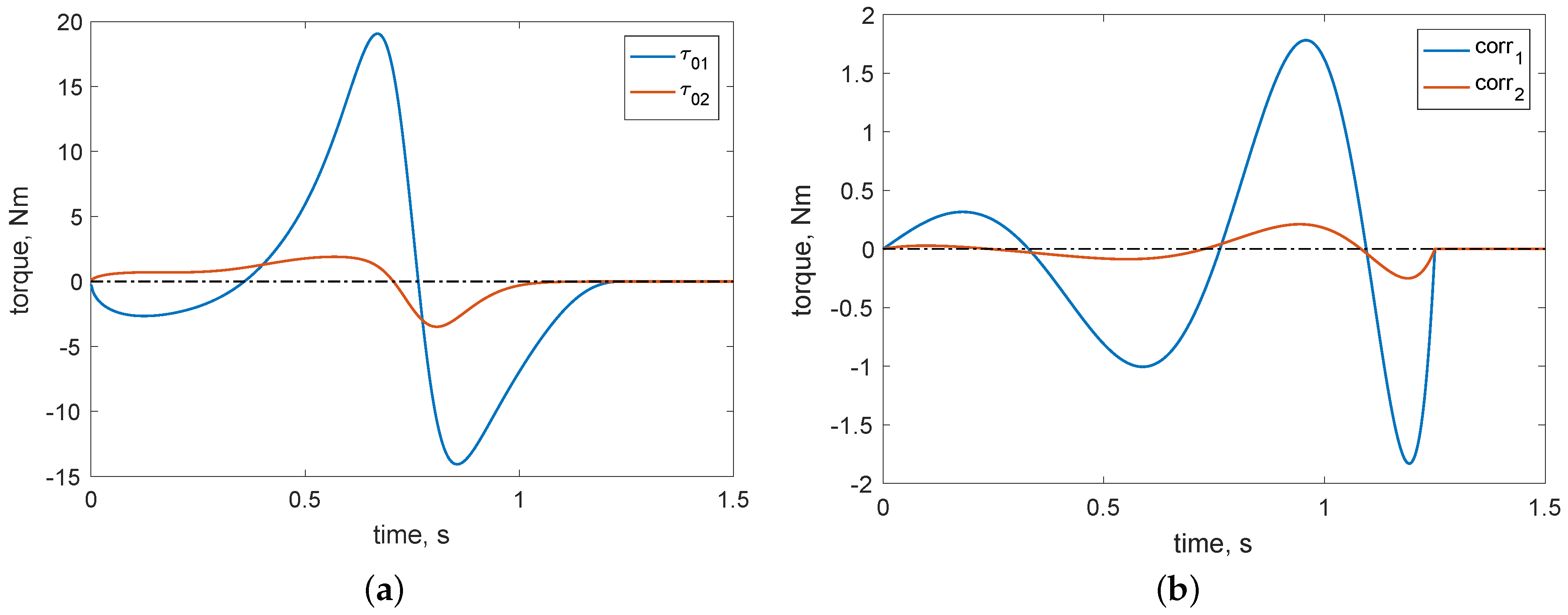
Figure 2a and Figure 3a show the torques ${\tau }_{0i}$ evaluated for the 2R rigid robot, while Figure 2b and Figure 3b display the second term of Equation (17) obtained as a result of the optimization problem.

The used coefficients of the feedback loops are $K_{P1}=25$ Nm, $K_{P2}=22$ Nm, $K_{D1}=0.42$ Nms and $K_{D2}=0.22$ Nms.

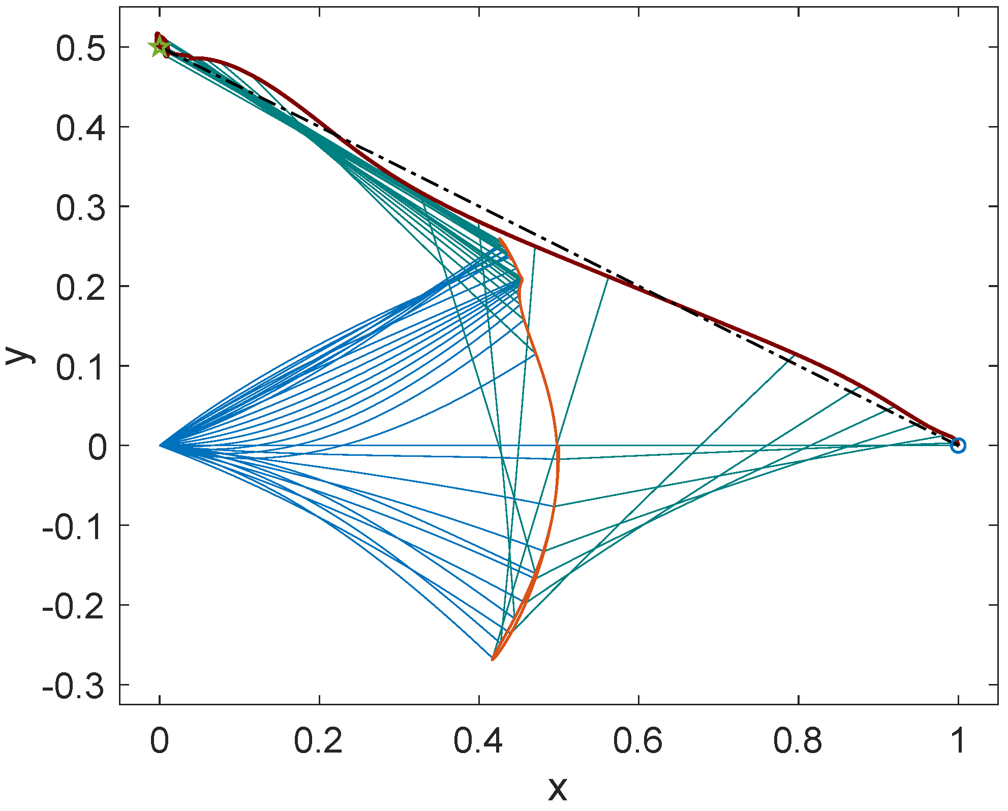
In Figure 4, Figure 5, Figure 6 and Figure 7 are compiled the results obtained for the two examined cases, respectively for the linear and the parabolic case.

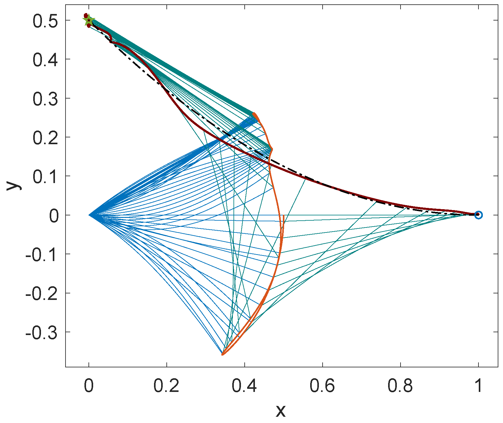
In particular, Figure 4 and Figure 6 show the reference path (dashed black line) for the tip of the arm in which the start and end points are highlighted with a circle and a star, respectively. These figures also exhibit the actual trajectories of the two ends of the links, as well as some intermediate deformed configurations for the links. The deformations of the links are clearly in the range of large deflections, and therefore, any linearization procedure is not allowed in the investigated cases.

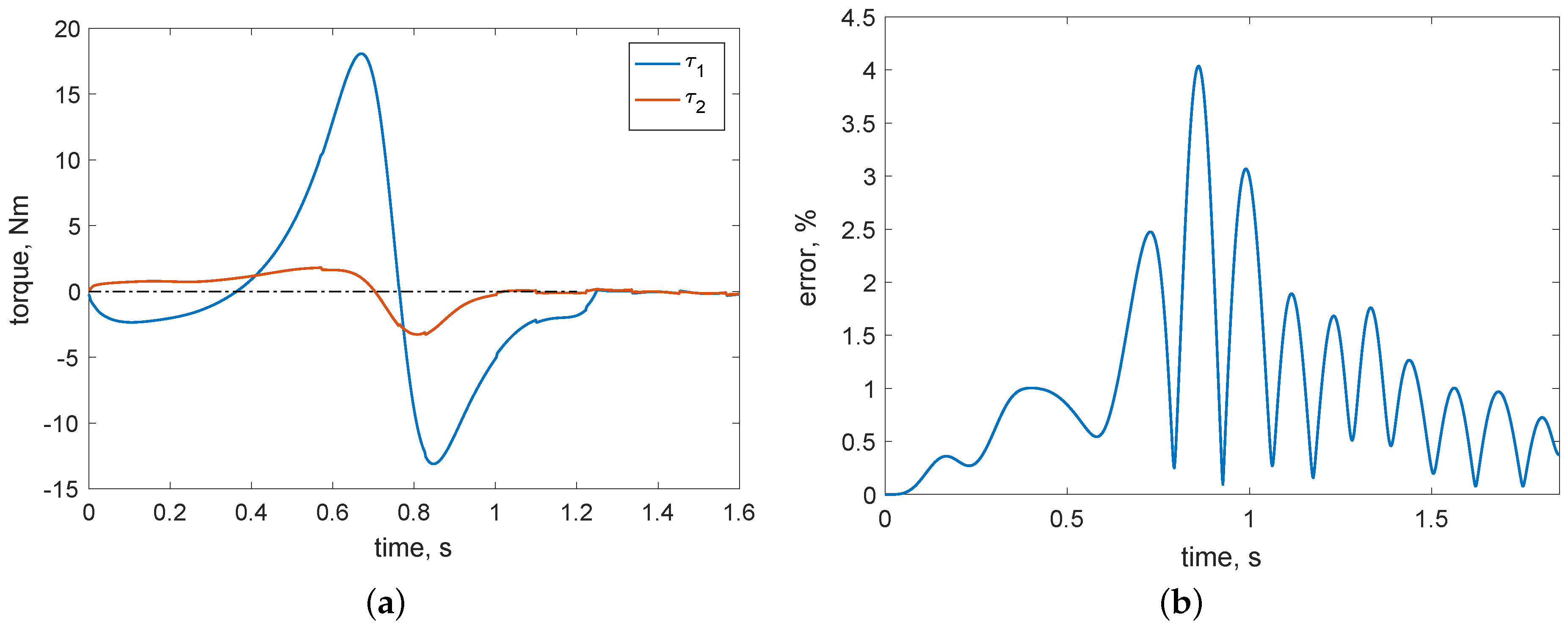
Figure 5a and Figure 7a display the actual joint torques resulting from the control strategy of a feedforward with an optimal input command and a feedback of the signals, angles and angular velocities, acquired from the joints. These plots evince the difference between the two joint torques, as well as the power required by the motors and therefore their size. Of course, once the time law (21) has been set, to limit the maximum torque that can be provided, it is possible to change the task time. Thus, we set the task times for the considered cases in order to limit the torques at reliable values.

Figure 5b and Figure 7b exhibit the tip error in following the desired trajectory for the three studied cases. We can see from the graphs that the errors normalized to the full length of the robotic arm were less than 4.5% despite the great deformability of the links and the shortness of the task time.

Table 1. Optimal torque coefficients for the linear trajectory case.

	${\mathit{a}}_0^{\left(\mathit{i}\right)}$	${\mathit{a}}_1^{\left(\mathit{i}\right)}$	${\mathit{a}}_2^{\left(\mathit{i}\right)}$	${\mathit{a}}_3^{\left(\mathit{i}\right)}$	${\mathit{a}}_4^{\left(\mathit{i}\right)}$	${\mathit{a}}_5^{\left(\mathit{i}\right)}$	${\mathit{a}}_6^{\left(\mathit{i}\right)}$
Link 1	113.65	−590.40	102.40	210.97	3612.9	−3800.3	−0.00178
Link 2	−0.1364	105.65	−780.47	1570.4	−848.80	−108.65	−0.01214

and

Table 2. Optimal torque coefficients for the parabolic trajectory case.

	${\mathit{a}}_0^{\left(\mathit{i}\right)}$	${\mathit{a}}_1^{\left(\mathit{i}\right)}$	${\mathit{a}}_2^{\left(\mathit{i}\right)}$	${\mathit{a}}_3^{\left(\mathit{i}\right)}$	${\mathit{a}}_4^{\left(\mathit{i}\right)}$	${\mathit{a}}_5^{\left(\mathit{i}\right)}$	${\mathit{a}}_6^{\left(\mathit{i}\right)}$	${\mathit{a}}_7^{\left(\mathit{i}\right)}$	${\mathit{a}}_8^{\left(\mathit{i}\right)}$
Link 1	0.8090	1.114	−11.239	−1.681	1.297	19.485	14.592	−6.116	−15.732
Link 2	0.2139	−1.434	2.659	0.0668	−9.700	10.966	3.453	−5.661	−0.2856

summarize the coefficients, obtained minimizing the functional J, to represent the torques in terms of the interpolation polynomial functions considered for the analyzed cases.

The order of the interpolating polynomial was fixed by increasing it subsequently until the error obtained by the optimization process stabilized. To perform the minimization, we employ a MATLAB code that makes use of the function fminsearch.

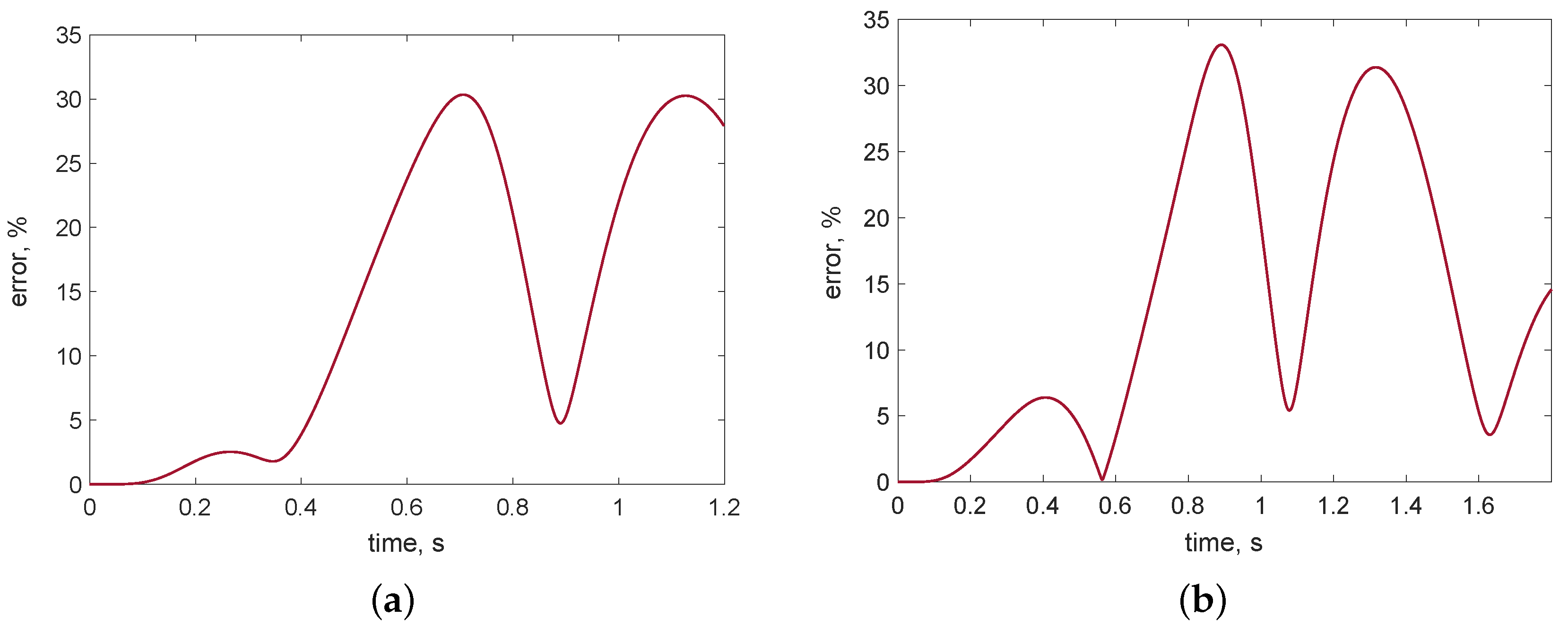
To estimate the efficiency of the proposed approach, we compare the used control strategy with a standard PD control with a feedback of the angular joints $({\vartheta }_i,{\dot{\vartheta }}_i)$ using a desired trajectory evaluated for the linear and parabolic rigid cases, respectively, Equations (20) and (22) and the time law (21). Figure 8 shows the relative tracking error of the manipulator tip in both examined cases with the PD feedback gains: $K_{P1}=25$ Nm, $K_{P2}=22$ Nm, $K_{D1}=4.2$ Nms and $K_{D2}=2.2$ Nms. The tracking performances obtained exhibit a maximum relative error of about 30%, much greater than the optimal pre-shaping input approach.

4. Conclusions

In this article, we propose a lumped parameters modeling approach for flexible robotic manipulators in the nonlinear regime. In this context, the method of the assumption of the modes, typically used, cannot be utilized because the hypotheses on which it is based are inadequate for the given problem. We propose to use this formulation for its great simplicity of modeling and for its intrinsic nonlinear nature, instead of the finite element method, which requires a greater modeling effort even if it has a faster convergence speed. Furthermore, an isogeometric formulation, still not fully affirmed as an alternative to the standard FEM, can also improve the results because at equal accuracy, it requires a lesser number of degrees of freedom and seems to be promising for further advances (see, e.g., [54,55,56] for recent developments).

The number of degrees of freedom that should be treated in the nonlinear case of large link deflections does not allow us to opt for a well-established control strategy such as online computed-torque; therefore, a different control approach must be developed. We present a control approach based on a pre-shaping input that, instead of using appropriately designed signal filters, produces a feedforward command signal for the motors using an optimal problem in which a functional, properly defined, is minimized on the basis of the positioning error of the end effector of the manipulator. In order to stabilize the response close to the desired one, a feedback signal is used together to make the system less sensitive to external disturbances. The employed control strategy is therefore more suitable to treat a greater number of degrees of freedom and can be implemented with minimal hardware equipment. The system considered is under-actuated, and therefore, it is not possible to obtain a perfect positioning of the manipulator tip. However, the simulated numerical cases show that under very strict operating conditions, it is possible to obtain a trajectory tracking with an error of less than about 4.5%. A comparison with a standard feedback PD control strategy shows that, with the optimal pre-shaping input, it is possible to achieve a better tip positioning.

The optimal problem in this paper has been solved numerically to explore the possibilities offered by the proposed method. The preliminary results achieved are quite encouraging, and therefore, as a future research direction, it would be interesting to address the optimal problem rigorously with the calculus of the variations and, in this way, characterize the minimum error obtainable accurately in the various operating conditions.

References

- Cannon, R.H., Jr.; Schmitz, E. Initial experiments on the end-point control of a flexible one-link robot. Int. J. Robot. Res. 1984, 3, 62–75. [Google Scholar] [CrossRef]
- Tosunoglu, S.; Lin, S.H.; Tesar, D. Accessibility and controllability of flexible robotic manipulators. J. Dyn. Syst. Meas. Control 1992, 114, 50–58. [Google Scholar] [CrossRef]
- Sayahkarajy, M.; Mohamed, Z.; Mohd Faudzi, A.A. Review of modeling and control of flexible-link manipulators. Proc. Inst. Mech. Eng. Part I J. Syst. Control Eng. 2016, 230, 861–873. [Google Scholar] [CrossRef]
- Önsay, T.; Akay, A. Vibration reduction of a flexible arm by time-optimal open-loop control. J. Sound Vib. 1991, 147, 283–300. [Google Scholar] [CrossRef]
- Meckl, P.; Seering, W. Experimental evaluation of shaped inputs to reduce vibration for a cartesian robot. J. Dyn. Syst. Meas. Control 1990, 112, 159–165. [Google Scholar] [CrossRef]
- Gregory, J.; Olivares, A.; Staffetti, E. Energy-optimal trajectory planning for robot manipulators with holonomic constraints. Syst. Control Lett. 2012, 61, 279–291. [Google Scholar] [CrossRef]
- Book, W.J. Controlled motion in an elastic world. J. Dyn. Syst. Meas. Control 1993, 115, 252–261. [Google Scholar] [CrossRef]
- Katzschmann, R.K.; Marchese, A.D.; Rus, D. Autonomous object manipulation using a soft planar grasping manipulator. Soft Robot. 2015, 2, 155–164. [Google Scholar] [CrossRef] [PubMed]
- Antman, S.S. Kirchhoff’s problem for nonlinearly elastic rods. Q. Appl. Math. 1974, 32, 221–240. [Google Scholar] [CrossRef] [Green Version]
- Steigmann, D.J.; Faulkner, M.G. Variational theory for spatial rods. J. Elast. 1993, 33, 1–26. [Google Scholar] [CrossRef] [Green Version]
- Greco, L.; Cuomo, M. Consistent tangent operator for an exact Kirchhoff rod model. Contin. Mech. Thermodyn. 2015, 27, 861–877. [Google Scholar] [CrossRef]
- Altenbach, H.; Bîrsan, M.; Eremeyev, V.A. Cosserat-type rods. In Generalized Continua from the Theory to Engineering Applications; Springer: Vienna, Austria, 2013; pp. 179–248. [Google Scholar]
- Eugster, S.R.; Hesch, C.; Betsch, P.; Glocker, C. Director-based beam finite elements relying on the geometrically exact beam theory formulated in skew coordinates. Int. J. Numer. Methods Eng. 2014, 97, 111–129. [Google Scholar] [CrossRef]
- Della Corte, A.; dell’Isola, F.; Esposito, R.; Pulvirenti, M. Equilibria of a clamped Euler beam (Elastica) with distributed load: Large deformations. Math. Models Methods Appl. Sci. 2017, 27, 1391–1421. [Google Scholar] [CrossRef]
- Spagnuolo, M.; Andreaus, U. A targeted review on large deformations of planar elastic beams: Extensibility, distributed loads, buckling and post-buckling. Math. Mech. Solids 2018. [Google Scholar] [CrossRef]
- Giorgio, I.; Della Corte, A.; Del Vescovo, D. Modelling flexible multi-link robots for vibration control: Numerical simulations and real-time experiments. Math. Mech. Solids 2017. [Google Scholar] [CrossRef]
- Low, K.H. Solution schemes for the system equations of flexible robots. J. Field Robot. 1989, 6, 383–405. [Google Scholar] [CrossRef]
- Du, H.; Lim, M.; Liew, K. A nonlinear finite element model for dynamics of flexible manipulators. Mech. Mach. Theory 1996, 31, 1109–1119. [Google Scholar] [CrossRef]
- Wang, Y.; Huston, R.L. A lumped parameter method in the nonlinear analysis of flexible multibody systems. Comput. Struct. 1994, 50, 421–432. [Google Scholar] [CrossRef]
- Šalinić, S. An improved variant of Hencky bar-chain model for buckling and bending vibration of beams with end masses and springs. Mech. Syst. Signal Process. 2017, 90, 30–43. [Google Scholar] [CrossRef]
- Yoshikawa, T.; Hosoda, K. Modeling of flexible manipulators using virtual rigid links and passive joints. Int. J. Robot. Res. 1996, 15, 290–299. [Google Scholar] [CrossRef]
- Konno, A.; Uchiyama, M. Vibration suppression control of spatial flexible manipulators. Control Eng. Pract. 1995, 3, 1315–1321. [Google Scholar] [CrossRef]
- Garcea, G.; Trunfio, G.A.; Casciaro, R. Mixed formulation and locking in path-following nonlinear analysis. Comput. Methods Appl. Mech. Eng. 1998, 165, 247–272. [Google Scholar] [CrossRef]
- Livesley, R. The equivalence of continuous and discrete mass distributions in certain vibration problems. Q. J. Mech. Appl. Math. 1955, 8, 353–360. [Google Scholar] [CrossRef]
- Leckie, F.A.; Lindberg, G.M. The effect of lumped parameters on beam frequencies. Aeronaut. Q. 1963, 14, 224–240. [Google Scholar] [CrossRef]
- Duncan, W.J. A critical examination of the representation of massive and elastic bodies by systems of rigid masses elastically connected. Q. J. Mech. Appl. Math. 1952, 5, 97–108. [Google Scholar] [CrossRef]
- Dell’Isola, F.; Bucci, S.; Battista, A. Against the fragmentation of knowledge: The power of multidisciplinary research for the design of metamaterials. In Advanced Methods of Continuum Mechanics for Materials and Structures; Springer: Singapore, 2016; pp. 523–545. [Google Scholar]
- Jawed, M.K.; Novelia, A.; O’Reilly, O.M. A Primer on the Kinematics of Discrete Elastic Rods; Springer: Cham, Switzerland, 2018. [Google Scholar]
- Zhang, H.; Wang, C.M.; Challamel, N. Buckling and vibration of Hencky bar-chain with internal elastic springs. Int. J. Mech. Sci. 2016, 119, 383–395. [Google Scholar] [CrossRef]
- Alibert, J.J.; Della Corte, A.; Seppecher, P. Convergence of Hencky-type discrete beam model to Euler inextensible elastica in large deformation: Rigorous proof. In Mathematical Modelling in Solid Mechanics; Springer: Singapore, 2017; pp. 1–12. [Google Scholar]
- Alibert, J.J.; Della Corte, A.; Giorgio, I.; Battista, A. Extensional Elastica in large deformation as Γ-limit of a discrete 1D mechanical system. Z. Angew. Math. Phys. 2017, 68. [Google Scholar] [CrossRef]
- Battista, A.; Della Corte, A.; dell’Isola, F.; Seppecher, P. Large deformations of 1D microstructured systems modeled as generalized Timoshenko beams. Z. Angew. Math. Phys. 2018, 69. [Google Scholar] [CrossRef]
- Khakalo, S.; Balobanov, V.; Niiranen, J. Modelling size-dependent bending, buckling and vibrations of 2D triangular lattices by strain gradient elasticity models: Applications to sandwich beams and auxetics. Int. J. Eng. Sci. 2018, 127, 33–52. [Google Scholar] [CrossRef]
- De Luca, A.; Mattone, R.; Oriolo, G. Control of underactuated mechanical systems: Application to the planar 2R robot. In Proceedings of the 35th IEEE Conference on Decision and Control, Kobe, Japan, 13 December 1996; IEEE: Piscataway, NJ, USA, 1996; Volume 2, pp. 1455–1460. [Google Scholar]
- De Luca, A.; Oriolo, G. Trajectory planning and control for planar robots with passive last joint. Int. J. Robot. Res. 2002, 21, 575–590. [Google Scholar] [CrossRef]
- De Luca, A.; Mattone, R.; Oriolo, G. Stabilization of an underactuated planar 2R manipulator. Int. J. Robust Nonlinear Control IFAC-Affil. J. 2000, 10, 181–198. [Google Scholar] [CrossRef]
- Mohamed, Z.; Martins, J.; Tokhi, M.; Da Costa, J.S.; Botto, M. Vibration control of a very flexible manipulator system. Control Eng. Pract. 2005, 13, 267–277. [Google Scholar] [CrossRef] [Green Version]
- Singhose, W.; Singer, N.; Seering, W. Comparison of command shaping methods for reducing residual vibration. In Proceedings of the European Control Conference, Rome, Italy, 5–8 September 1995; pp. 1126–1131. [Google Scholar]
- De Luca, A.; Caiano, V.; Del Vescovo, D. Experiments on Rest-to-rest Motion of a Flexible Arm. In Experimental Robotics VIII; Springer: Berlin, Germany, 2003; pp. 338–349. [Google Scholar]
- Pepe, G.; Carcaterra, A.; Giorgio, I.; Del Vescovo, D. Variational Feedback Control for a nonlinear beam under an earthquake excitation. Math. Mech. Solids 2016, 21, 1234–1246. [Google Scholar] [CrossRef]
- Boscariol, P.; Gasparetto, A. Model-based trajectory planning for flexible-link mechanisms with bounded jerk. Robot. Comput.-Integr. Manuf. 2013, 29, 90–99. [Google Scholar] [CrossRef]
- Boscariol, P.; Gasparetto, A. Optimal trajectory planning for nonlinear systems: Robust and constrained solution. Robotica 2016, 34, 1243–1259. [Google Scholar] [CrossRef]
- Turco, E. Discrete is it enough? The revival of Piola–Hencky keynotes to analyze three-dimensional Elastica. Contin. Mech. Thermodyn. 2018. [Google Scholar] [CrossRef]
- Rubinstein, D. Dynamics of a flexible beam and a system of rigid rods, with fully inverse (one-sided) boundary conditions. Comput. Methods Appl. Mech. Eng. 1999, 175, 87–97. [Google Scholar] [CrossRef]
- Wang, C.M.; Zhang, H.; Gao, R.P.; Duan, W.H.; Challamel, N. Hencky bar-chain model for buckling and vibration of beams with elastic end restraints. Int. J. Struct. Stab. Dyn. 2015, 15. [Google Scholar] [CrossRef]
- Dell’Isola, F.; Giorgio, I.; Pawlikowski, M.; Rizzi, N.L. Large deformations of planar extensible beams and pantographic lattices: Heuristic homogenization, experimental and numerical examples of equilibrium. Proc. R. Soc. A 2016, 472. [Google Scholar] [CrossRef]
- Turco, E.; dell’Isola, F.; Cazzani, A.; Rizzi, N.L. Hencky-type discrete model for pantographic structures: Numerical comparison with second gradient continuum models. Z. Angew. Math. Phys. 2016, 67. [Google Scholar] [CrossRef]
- Altenbach, H.; Eremeyev, V.A. On the constitutive equations of viscoelastic micropolar plates and shells of differential type. Math. Mech. Complex Syst. 2015, 3, 273–283. [Google Scholar] [CrossRef] [Green Version]
- Cuomo, M. Forms of the dissipation function for a class of viscoplastic models. Math. Mech. Complex Syst. 2017, 5, 217–237. [Google Scholar] [CrossRef] [Green Version]
- Dietrich, L.; Lekszycki, T.; Turski, K. Problems of identification of mechanical characteristics of viscoelastic composites. Acta Mech. 1998, 126, 153–167. [Google Scholar] [CrossRef]
- De Wit, C.C.; Olsson, H.; Astrom, K.J.; Lischinsky, P. A new model for control of systems with friction. IEEE Trans. Autom. Control 1995, 40, 419–425. [Google Scholar] [CrossRef] [Green Version]
- Buechner, S.; Schreiber, V.; Amthor, A.; Ament, C.; Eichhorn, M. Nonlinear modeling and identification of a dc-motor with friction and cogging. In Proceedings of the Industrial Electronics Society, IECON 2013-39th Annual Conference of the IEEE, Vienna, Austria, 10–13 November 2013; IEEE: Piscataway, NJ, USA, 2013; pp. 3621–3627. [Google Scholar]
- Dawson, D.M.; Abdallah, C.T.; Lewis, F.L. Robot Manipulator Control: Theory and Practice; CRC Press: Boca Raton, FL, USA, 2003. [Google Scholar]
- Greco, L.; Cuomo, M.; Contrafatto, L.; Gazzo, S. An efficient blended mixed B-spline formulation for removing membrane locking in plane curved Kirchhoff rods. Comput. Methods Appl. Mech. Eng. 2017, 324, 476–511. [Google Scholar] [CrossRef]
- Cazzani, A.; Malagù, M.; Turco, E. Isogeometric analysis of plane-curved beams. Math. Mech. Solids 2016, 21, 562–577. [Google Scholar] [CrossRef]
- Niiranen, J.; Balobanov, V.; Kiendl, J.; Hosseini, S. Variational formulations, model comparisons and numerical methods for Euler–Bernoulli micro-and nano-beam models. Math. Mech. Solids 2017. [Google Scholar] [CrossRef]
Figure 1.
Discrete system for the planar two-link flexible robot.
Figure 2.
Linear trajectory case: (a) reference rigid torques; (b) correction torques.
Figure 3.
Parabolic trajectory case: (a) reference rigid torques; (b) correction torques.
Figure 4.
Stroboscopic motion for linear trajectory case.
Figure 5.
Linear trajectory case: (a) actual torques; (b) relative tracking error for the tip.
Figure 6.
Stroboscopic motion for the parabolic trajectory case.
Figure 7.
Parabolic trajectory case: (a) actual torques; (b) relative tracking error for the tip.
Figure 8.
Relative tracking error for the tip with collocated PD control: linear trajectory case (a); parabolic trajectory case (b).