Hyperspectral Anomaly Detection via Background Estimation and Adaptive Weighted Sparse Representation


Science and Technology on Automatic Target Recognition Laboratory, National University of Defense Technology, Changsha 410073, China
*
Author to whom correspondence should be addressed.
Remote Sens. 2018, 10(2), 272; https://0-doi-org.brum.beds.ac.uk/10.3390/rs10020272
Submission received: 10 January 2018
/
Revised: 2 February 2018
/
Accepted: 8 February 2018
/
Published: 10 February 2018
(This article belongs to the Section Remote Sensing Image Processing)
Abstract
:Anomaly detection is an important task in hyperspectral imagery (HSI) processing. It provides a new way to find targets that have significant spectral differences from the majority of the dataset. Recently, the representation-based methods have been proposed for detecting anomaly targets in HSIs. It is essential for this type of method to construct a valid background dictionary to distinguish anomaly and background accurately. In this paper, a novel hyperspectral anomaly detection method based on background estimation and adaptive weighted sparse representation has been proposed. Firstly, to obtain the effective background dictionary without anomaly information, a new background dictionary construction strategy is designed. Secondly, the sparse representation based on the constructed background dictionary is utilized on the dataset. Anomalies and background are distinguished through the response of the residual matrix. Thirdly, the residual matrix is weighted adaptively from global and local domains, which makes anomalies and background more discriminative. An important advantage of the proposed method is that it considers the properties of anomalies in both spectral and spatial domains. Experiments on three HSI datasets reveal that our proposed method achieves an outstanding detection performance compared with the other anomaly detection algorithms.
1. Introduction
Hyperspectral sensors capture hundreds of narrow and contiguous spectral bands of about 10 nm wide and span the visible, near-infrared and mid-infrared of the spectrum. Due to its rich information in the spectral dimension, hyperspectral imagery (HSI) has drawn more and more attention in the field of remote sensing [1,2,3,4,5]. Target detection aims to discriminate the specific target pixels from various of backgrounds, which is one of the most significant applications in HSI [6,7] processing. In most cases, the a priori information about the spectrum of the target of interest is difficult to obtain, so the target detection technique with no a priori information, known as anomaly detection, is widely used in practical situations [4,8,9].
Anomalies usually refer to objects with a spot of pixels (even subpixels) that have significant spectral differences from the homogenous background. In recent decades, a large number of anomaly detection methods has been proposed, and among them, the Reed–Xiaoli detector (RX) [10] is a well-known benchmark algorithm. It assumes that the background can be modeled by a multivariate Gaussian distribution, then the Mahalanobis distance between the test pixel and the background model is calculated. By comparing with a predefined threshold, it can be determined whether the test pixel belongs to background or anomaly. Although RX has high efficiency and mathematically tractable, it still has two main problems. The first one is that the multivariate Gaussian distribution is not always suitable to describe the background in the real HSI, especially when the background compositions are complicated. The second one is that the samples chosen as background always contains anomaly pixels, which will contaminate the background model and influence the detection performance. Therefore, a series of improved RX-based algorithms has been proposed, such as the cluster-based anomaly detection method (CBAD) [11], which applies the clustering strategy on the HSI and then executes the detection process in each cluster. The subspace RX (SSRX) [12,13] applies principal component analysis (PCA) on the HSI and runs the RX detector on a limited number of PCA bands. The kernel-RX (KRX) [14] and cluster kernel-RX (CKRX) [15] project the original input space to a high-dimensional feature space, which belong to nonlinear versions of RX. Besides, for a more accurate characterization of the complicated background, some algorithms based on the non-Gaussian model have been proposed, such as the anomaly detection algorithm based on the elliptically-contoured distribution (ECD) [16]. Some methods focus on mitigating the anomaly contamination in background estimation, such as the random selection-based anomaly detector (RSAD) [17], the robust nonlinear anomaly detection (RNAD) [18], the blocked adaptive computationally-efficient outlier nominator (BACON) [19] and the discriminative metric learning-based anomaly detection (DMLAD) [20]. Moreover, some algorithms consider the spectral differences in neighboring pixels and apply the detection in the local window, such as dual window-based Eigen separation transform (DWEST) [21] and multiple-window anomaly detection (MWAD) [22].
In recent years, representation theory has been introduced to the field of hyperspectral anomaly detection, and some related algorithms have been proposed. For instance, the collaborative representation-based detector (CRD) [23] utilizes the neighboring pixels to collaboratively represent the pixel under test. The background joint sparse representation detector (BJSRD) [24] measures the length of the matched projection on the orthogonal complementary background subspace for the pixel under test by joint sparse representation (JSR) [25,26]. The low-rank and sparse representation-based detector (LRASR) [27] uses the low-rank representation with a sparsity-inducing regularization term in the coefficients to model the background part. These approaches avoid the explicit assumption of the statistical distribution for the background and exploit the characteristics in the data implicitly. However, for both the sparse representation-based detector and CRD, the detection capability has a high correlation with the used dictionary; in other words, a low detection rate may be obtained if the background is contaminated by anomalies. Researchers have proposed different strategies to construct the background dictionary. A common way is the dual-window method; in addition, the method of choosing neighboring pixels based on JSR is used in [24], and a learned dictionary using sparse coding is applied in [28].
In this paper, a novel hyperspectral anomaly detection method based on background estimation and adaptive weighted sparse representation is proposed. Considering the great difference between anomalies and background in spectra, we first apply the sequential maximum angle convex cone (SMACC) endmember extraction method on the HSI. There are two main purposes of this process. The first is to find those extreme spectra in the data, denoted as endmembers, and the second is to determine each endmember’s abundance fraction in each pixel, i.e., to obtain a series of abundance fraction maps of the endmembers. Based on the conventional definition of the aforementioned anomaly target, it can be considered that an anomaly target may exist if the abundance fractions of one specific endmember in a spot area are extremely high. Therefore, in our proposed method, a structure element with a predefined size is introduced, which slides in each abundance fraction map and aims to find all regions with the anomaly characteristic, and we consider that all potential anomaly targets are contained in them. Then, a random selection procedure is applied in the rest of the pixels to construct the background dictionary. This process focuses on minimizing the contamination of the anomalies. In the next step, the sparse representation based on the background dictionary is used on all pixels, and the residual between each original spectrum and the reconstructed spectrum is obtained simultaneously, which is the metric to discriminate anomaly and background. Moreover, to further improve the discrimination between anomalies and background, an adaptive weighted strategy in both global and local domains is introduced in our proposed algorithm.
The remainder of this paper is organized as follows. Section 2 briefly reviews the basic theories of the related methodologies. Section 3 describes the proposed anomaly detection method in detail. The experiment results of the proposed method on several HSI datasets are presented in Section 4. Finally, the conclusion is drawn in Section 5.
2. Brief Review of the Related Methodologies
In this section, we introduce the SMACC endmember model and the sparse representation theory briefly. They play significant roles in our proposed anomaly detection method.
2.1. SMACC Endmember Model
Endmembers refer to the spectral signatures of pure components in the HSI [1]. The SMACC endmember model was proposed by Gruninger et al. [29], which provided a fast and automatic method to find spectral endmembers in the HSI.
A HSI dataset can be represented by a matrix , where denotes the bands of the spectrum and is pixels in the image. Therefore, is the -th band of the -th pixel, and it can be expanded as follows:
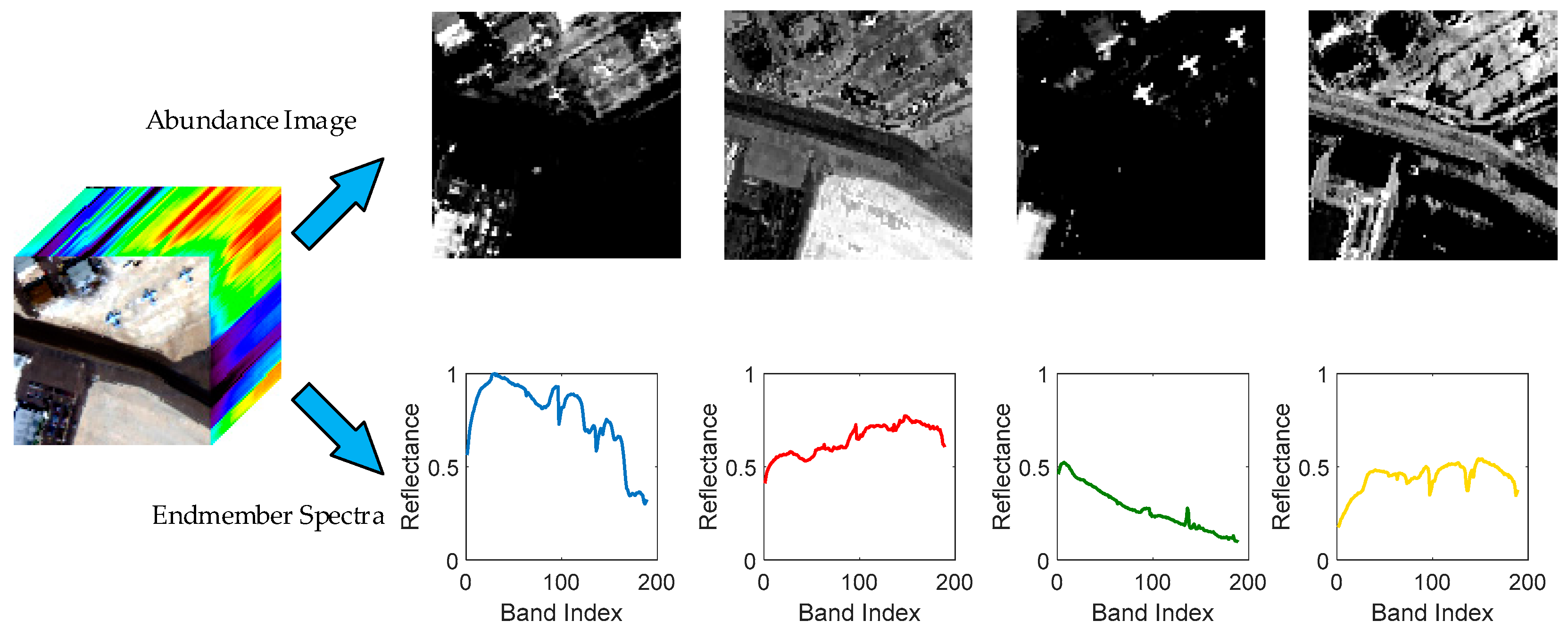
where is the expansion length, is a basis matrix containing columns and each of them is an endmember spectrum. The matrix contains an abundance of each endmember for each pixel. represents the residual matrix. The SMACC method uses a convex cone model to select the spectral combination to form the basis matrix. In general, the spectra of an HSI dataset represent its radiance or reflectance, so the endmembers must satisfy a positive constraint. Under the constraint, the spectra selected by SMACC are the extreme ones in the HSI dataset. The extreme vector determines a convex cone, which is defined as the first endmember. The residuals refer to the components that lie outside of the convex cone. Then, a constrained oblique projection is used on the previous convex cone to derive the next endmember. The purpose is to find the vector outside the convex cone that has the largest distance from the cone, then the new endmember is added into the basis, and the convex cone is updated. This process is terminated until the new endmember lies in the previous convex cone or the number of endmembers reaches a setting threshold. The result provided by SMACC includes the endmember spectra, as well as the abundance image of each endmember.
The abundance image indicates the contribution of the corresponding endmember for each pixel. A simple example is demonstrated in Figure 1.
2.2. Sparse Representation
In the sparse representation theory, a test signals can be well estimated by a sparse linear combination of the training samples (dictionary) [30]. Suppose a test sample in the HSI dataset is ; it is a vector with dimensions, which is the number of spectral bands. In addition, the training samples can be denoted as , and is the number of samples. Then, the test sample can be represented as follows:
where is the dictionary with the size of and is a sparse vector for which most of the entries are equal to zero. The sparse vector can be obtained by solving the optimization problem:
where is the -norm; it is called the sparsity level of the vector, which refers to the number of nonzero entries in the vector [31]. Because of the existence of estimation errors in the observed data, the optimization problem can be converted to minimizing the estimation error at a specific sparsity level through solving:
where is an upper bound of the sparsity level [32]; the above problem can be solved by greedy pursuit algorithms such as matching pursuit algorithm (MP) [33] or the orthogonal matching pursuit algorithm (OMP) [34].
3. Proposed Method
This section gives the details of the proposed anomaly detection method. In the first part, a background dictionary construction strategy is introduced. In the second part, the adaptive weighted sparse representation method is described. Finally, the framework of the detection method is given in the third part.
3.1. Background Dictionary Construction
In the anomaly detection task, we lack the targets’ a priori information, such as their spectral signatures and their distributions. In the first step of our proposed method, we need to construct an over-complete background dictionary, and all samples contained in the dictionary are background pixels. Assume is an arbitrary test pixel and is the background dictionary, then the hypothesis of the presence of anomalies can be provided as follows:
where is the background sparse vector, is the anomaly spectral signature contained in and is the additive noise signal, which cannot be ignored in the real situations. In the case of , it can be considered that the anomaly spectral signature has a significant influence on ; thus, the spectrum in exhibits a large difference from either pure background spectra or mixed background spectra. Let be the residual of the background dictionary , i.e.,
then will be relatively large if is an anomaly pixel, otherwise it will be small enough. Based on this view, it is essential to construct the background dictionary in the unsupervised state for distinguishing anomalies from the background effectively.
The main issue of the background dictionary construction is determining pixels belonging to the background accurately and avoiding anomalies being misclassified into the background. The problem of background estimation in the HSI has been researched in depth, and a typical approach is the dual-window strategy. For a test pixel , an outer window and an inner window are established centered on it. The criteria to judge whether is anomaly or background is based on the proximity between outer window pixels and . It will be close enough if is a background pixel, or else it will have an obvious difference. However, this method has the limitation that if some anomaly spectra exist in the outer window, it can hardly distinguish the test pixel as an anomaly. In our method, the joint slide structure element and protective-window strategy is proposed to prevent the occurrence of this situation.
For an HSI dataset , a group of endmember spectra and the corresponding abundance images are obtained by applying the SMACC endmember extraction model firstly. Assume there are endmembers, which can be determined by the eigenvalue likelihood maximization (ELM) method [35]. Then, the endmember spectra set can be denoted as , and the abundance image set is denoted as . For abundance image , we set an abundance fraction threshold . Considering that pixels with values larger than have a valid contribution with respect to , they can be called valid endmember pixels (VEPs), and the others are called invalid endmember pixels (IEPs). Therefore, if exists as a large region consisting of VEPs, then it is reasonable to determine as a background endmember, otherwise can be determined as an anomaly endmember. To select the anomaly endmembers and the corresponding abundance images, a morphological structure element is created. Usually, the shape of can be set as a circle or square as needed; its size is set to . Since there is no a priori information about the anomaly targets, so the size needs to be determined empirically. The ideal situation is that it is lightly larger than the potential anomaly targets. This selecting procedure is executed through sliding on each abundance image.
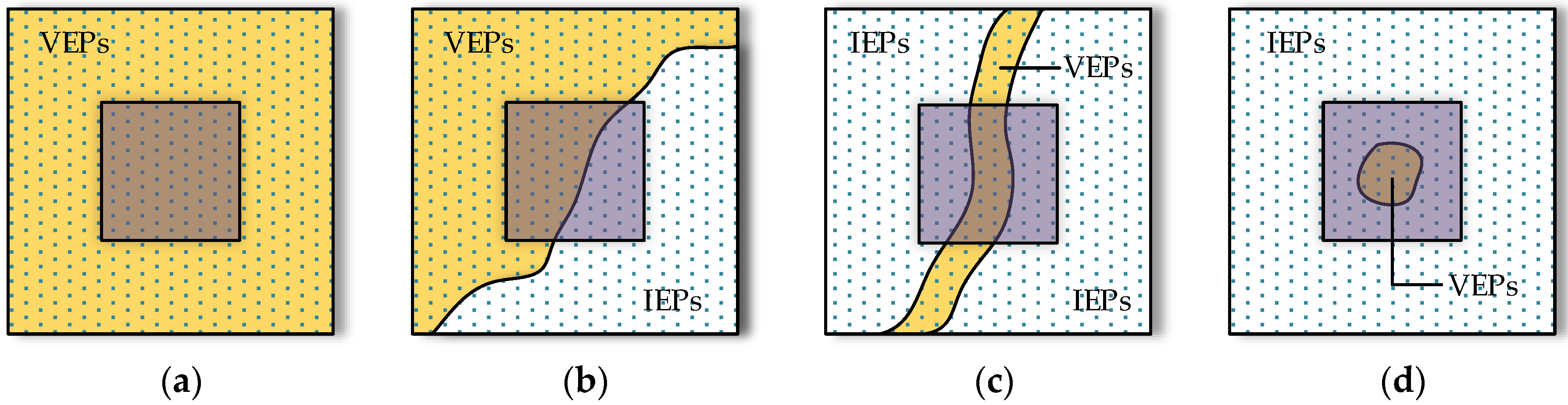
Some possible cases in the sliding process are given in Figure 2, and the is demonstrated as a purple square. (1) All pixels in the domain of are VEPs; see Figure 2a. This case happens when is in the background region, and the current endmember can be deemed as the background endmember. (2) A part of pixels are occupied by VEPs in ; see Figure 2b. This case always happens on the edge of the background. (3) Pixels in a striped area in belong to VEPs; see Figure 2c. This case happens if the endmember is extracted from roads or rivers. (4) Only a tiny part of the pixels are VEPs and centered on the ; see Figure 2d. This case can happen if the endmember belongs to the anomaly endmember group. It is noteworthy the Case 4 can exist with the other cases in one abundance image simultaneously, due to the discontinuity of the VEPs. Therefore, we consider an anomaly endmember to be confirmed when only Case 4 exists in its abundance image.
By the method provided hereinabove, assume we obtain anomaly endmembers’ abundance images, denoted as , and there are in total VEPs; the corresponding elements set in can be represented as ; for each , a protective window with the same size as is constructed centered on it. The aim is to include those anomaly pixels with low anomaly abundance fractions that may be missed in the previous step. Then, the anomaly regions can be denoted as , and the background elements set is defined as follows:
To reduce the dimensions of the dictionary and to improve computational efficiency, we randomly select a part of the elements in HB as the background dictionary atoms. Finally, the over-complete background dictionary DB is obtained.
3.2. Adaptive Weighted Sparse Representation
As described above, the background over-complete dictionary DB performs as the basis vector to complete the spectral reconstruction. The coefficients of DB form a sparse vector, which is depicted in Equation (4). In this paper, the problem in Equation (4) is solved by the OMP algorithm. The main idea of this algorithm is to choose the atom in DB by the greedy iterative method, which makes the chosen atom and the present redundant vector related to the greatest extent and subtracts the related part from DB. It will terminate if one of the following cases happens: (1) a predefined sparsity level is reached in the iteration process; (2) the residual becomes small enough [36]. Since the residual is the judgment criteria in our proposed method, Case 2 needs to be removed, and the sparsity level K0 is the only parameter in the sparse representation procedure. The detailed influences of the sparsity level K0 are further analyzed in the experiments part part of parameter analysis.
For those anomaly pixels with low anomaly abundance fractions, they can be well estimated by the OMP algorithm, which means they have sufficiently small residuals; thus, it becomes hard to obtain satisfactory detection performance on these pixels. To overcome this problem, an adaptive weighted method is introduced in our proposed method. Considering we have obtained the anomaly endmembers’ abundance images set AE in the previous step, each abundance image in AE reflects the corresponding anomaly endmember’s abundance fraction in each pixel. Therefore, we sum up images in AE and obtain the anomaly weights matrix. If one pixel belongs to an anomaly, then its value in the anomaly weights matrix will be relatively large, otherwise it will be relatively small. Therefore, for a test pixel x, the residual provided by Equation (6) can be modified as follows:
where Hx(1 ≤ Hx ≤ H) is the corresponding number of x in the image. The adaptive weight item in Equation (8) enhances the gaps between anomaly pixels and background pixels. Which can improve the detection performance to some extent. In addition, considering that the centers of anomaly targets usually have significantly high values in the anomaly weights matrix, then a local weighted strategy is designed based on this characteristic. Firstly, a search process is applied on the anomaly weights matrix to find a series of pixels with the top high values, and a lower bound threshold L1 is set to choose these pixels. It needs to ensure that all these pixels are discrete in locations, or else the max one is selected from its neighbors. In the unsupervised condition, we deem these pixels larger than L1 as the centers of potential anomaly targets. For each center pixel, the structure element SE is constructed centered on it, and all pixels in SE can be treated as suspected anomaly pixels. All these pixels are multiplied by an expansion coefficient λ, then Equation (8) updates as:
Equation (9) considers the global weights and local weights simultaneously, which can improve the discrimination between anomalies and background in a further step. Finally, we describe the whole procedure of adaptive weighted sparse representation in summary, which is shown in Procedure 1 as follows:
| Procedure 1. Adaptive weighted sparse representation. |
| Input: original HSI dataset H; background over-complete dictionary DB; anomaly endmembers’ abundance images set AE. Output: residual matrix X. Initialize: lower bound threshold L1; structure element SE; expansion coefficient λ; sparsity level K0.
|
3.3. Framework of the Proposed Method
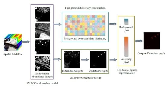
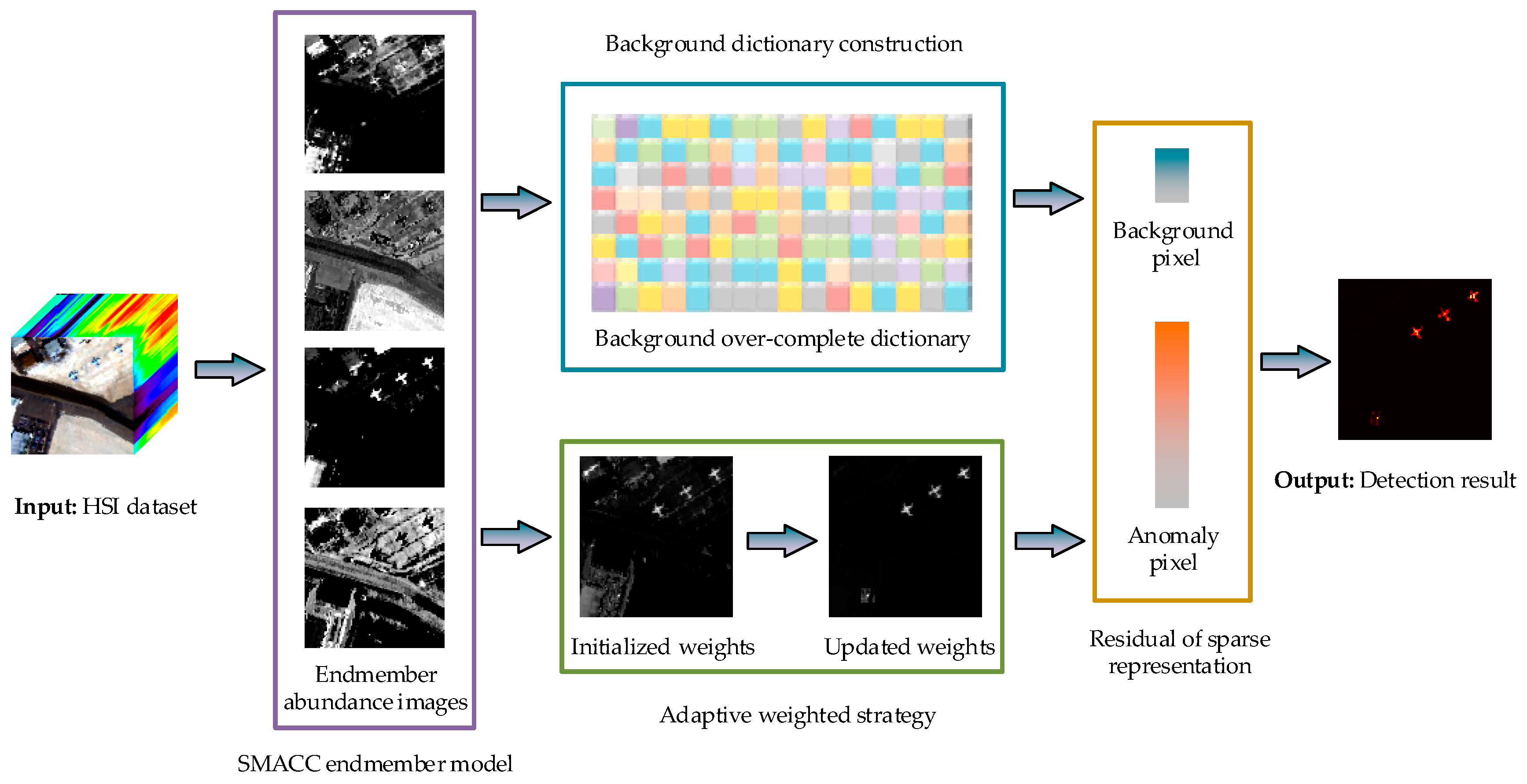
The visual framework of the proposed detection method is shown in Figure 3, which is called the background estimation and adaptive weighted sparse representation algorithm (BE-AWSR). The main idea of the algorithm is to distinguish anomalies from the background based on the residuals of sparse representation. To obtain a better detection performance, an adaptive weighted strategy is added in the framework. The main steps of the BE-AWSR algorithm can be illustrated as follows:
Step (1): Apply the SMACC endmember model on the input HSI dataset, and obtain the endmember abundance images set;
Step (2): Select anomaly endmember abundance images and estimate regions belonging to the background, then construct the background over-complete dictionary;
Step (3): Create the anomaly weights matrix based on the anomaly endmembers’ abundance images and the local anomaly characteristic;
Step (4): Join the anomaly weights matrix and sparse representation to obtain the residual matrix.
4. Experimental Results and Analysis
In this section, the effectiveness of the proposed method is evaluated on three HSI datasets. The first one is a synthetic HSI dataset created through implanting anomaly spectra into the specific locations. The second one is a real HSI dataset with a relatively simple background distribution. The last one is another real HSI dataset with a complex background distribution. For comparison, a series of existing state-of-the-art anomaly detection algorithms is used as benchmarks in the experiments, including global RX (GRX) [10], local RX (LRX) [37], kernel-RX (KRX) [14], CBAD [11], subspace RX (SSRX) [12,13], DWEST [21], BJSRD [24] and CRD [23]. Furthermore, the influences of different parameters settings on each HSI dataset are discussed in detail. All the experiments are implemented on a computer with an Intel Core i5-5200U CPU at 2.20 GHz, 12-GB RAM and 64-bit Windows 10 OS. Intel Core i5-5200U Central Processing Unit (CPU) at 2.20 GHz, 12-GB Random Access Memory (RAM) and 64-bit Windows 10 Operating System (OS).
4.1. Dataset Description
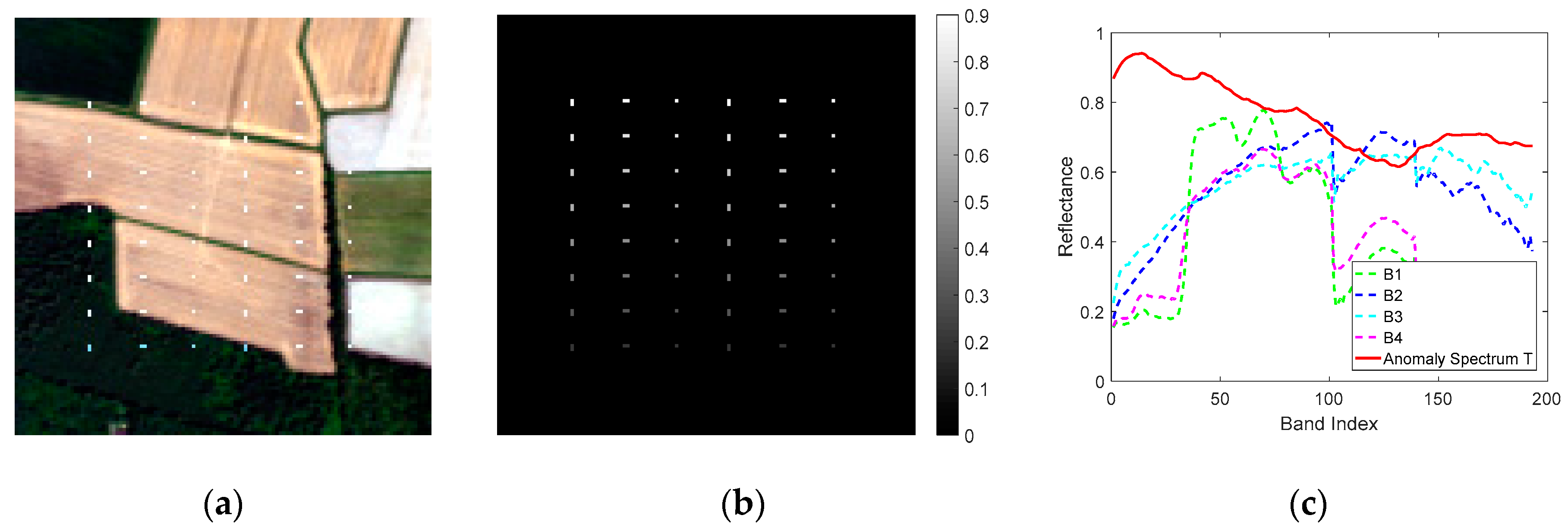
The first dataset is a synthetic image generated from a Hyperion dataset, which covers an agricultural area. The original dataset has a spectral resolution of 10 nm and a spatial resolution of 30 m, with 242 spectral bands in the VNIR-SWIR range (400–2500 nm). In our experiment, the low-SNR bands and the water vapor absorption bands are removed, and 193 bands are used in total. The selected portion of the scene (illustrated in Figure 4) has a size of 120 × 120.
In the experiment, we adopt a target implantation method to simulate the anomaly targets in the considered scene. The aim of using this technique is to evaluate the performances of detection algorithms in a totally controlled environment [38]. Based on the linear mixed model, a synthetic anomaly pixel with spectrum z is generated through implanting a desired target spectrum t with a specific abundance fraction f into a given background pixel with spectrum b as follows [39,40]:
The background land cover in the scene mainly includes four types of vegetation, as shown in Figure 4a. Meanwhile, in order to generate the simulated anomaly targets, 48 panels are embedded in the image with eight rows and six columns. The sizes of the panels in each column are as follows (in pixels): 2 × 1, 1 × 2, 1 × 1, 2 × 1, 1 × 2, 1 × 1, respectively. One kind of anomaly spectrum is selected to implant into each pixel of each panel using Equation (10); the abundance fraction f is 0.9, 0.8, 0.7, 0.6, 0.5, 0.4, 0.3 and 0.2 in each row, respectively. The distributions of anomaly targets and details about their sizes and abundance fractions are shown in Figure 4b. There are 80 anomaly pixels in total, and they account for 0.56% in the whole image approximately. In addition, Figure 4c shows the spectra of four types of main backgrounds (denoted as B1, B2, B3 and B4) and the anomaly spectrum (denoted as T Anomaly Spectrum T).
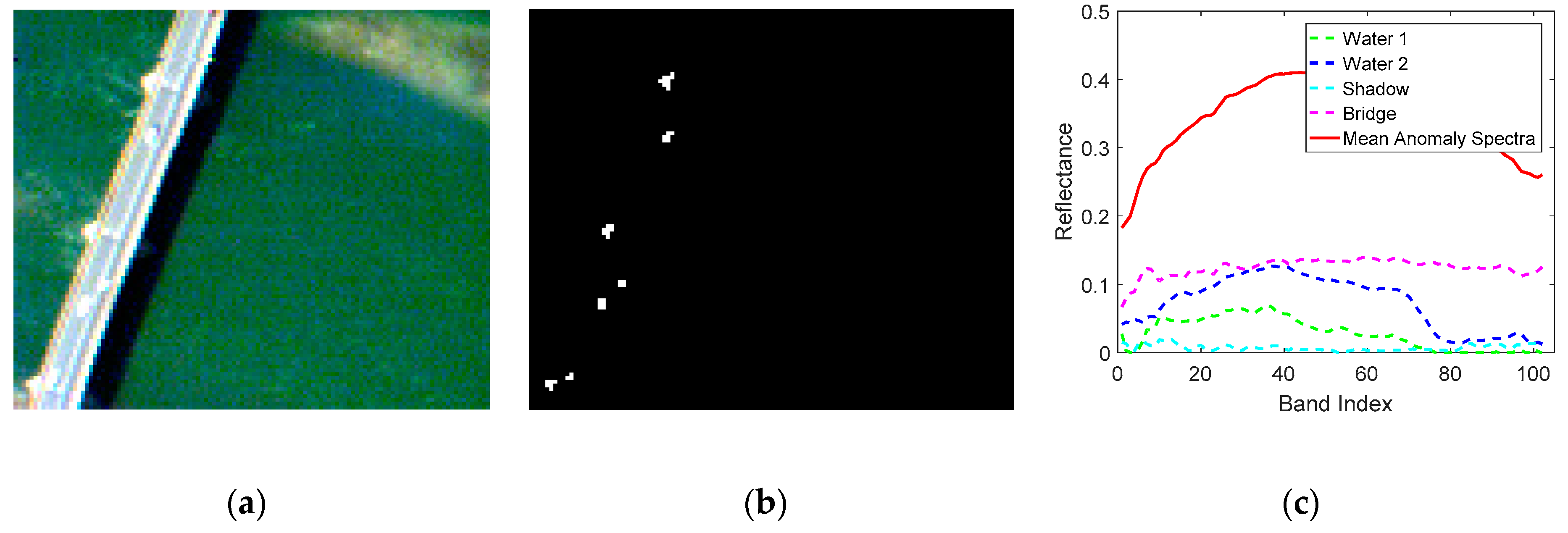
The second dataset was acquired by the Reflective Optics Spectrographic Imaging System airborne instrument (ROSIS) from Pavia city, Italy. The sensor has a spatial resolution of 1.3 m and contains 115 spectral bands ranging from 430–860 nm in wavelength. After removal of the noisy bands, 103 bands are used. The image scene in our experiment is comprised of 108 × 120 pixels, as shown in Figure 5a. The main backgrounds covered in the dataset are water and bridge, and there are approximately 43 anomaly pixels, which represent vehicles on the bridge, as well as bare soil near the bridge pier. The distributions of anomaly pixels are shown in Figure 5b. Besides, the spectra of main backgrounds and anomaly targets are illustrated in Figure 5c.
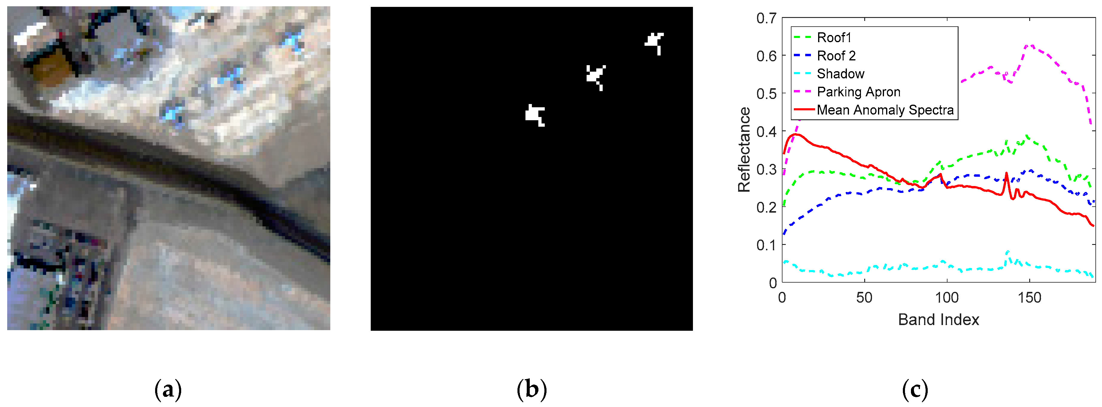
The third dataset was collected by the Airborne Visible/Infrared Imaging Spectrometer (AVIRIS) from the San Diego airport area, San Diego, CA, USA. This dataset has 224 spectral bands ranging from 370–2510 nm in wavelength, with a spatial resolution of 3.5 m per pixel. In the experiment, the low-SNR and water vapor absorption bands (1–6, 33–35, 97, 107–113, 153–166 and 221–224) are eliminated, and 189 bands are used. The size of the image scene is 100 × 100, and the main backgrounds include roof, shadow and parking apron; besides, three airplanes in the top right corner of the image are considered as anomaly targets, as shown in Figure 6a. There are 58 anomaly pixels in total, and their distributions are shown in Figure 6b. Figure 6c demonstrates the spectra of the main backgrounds and three anomaly targets in the scene.
4.2. Detection Performance
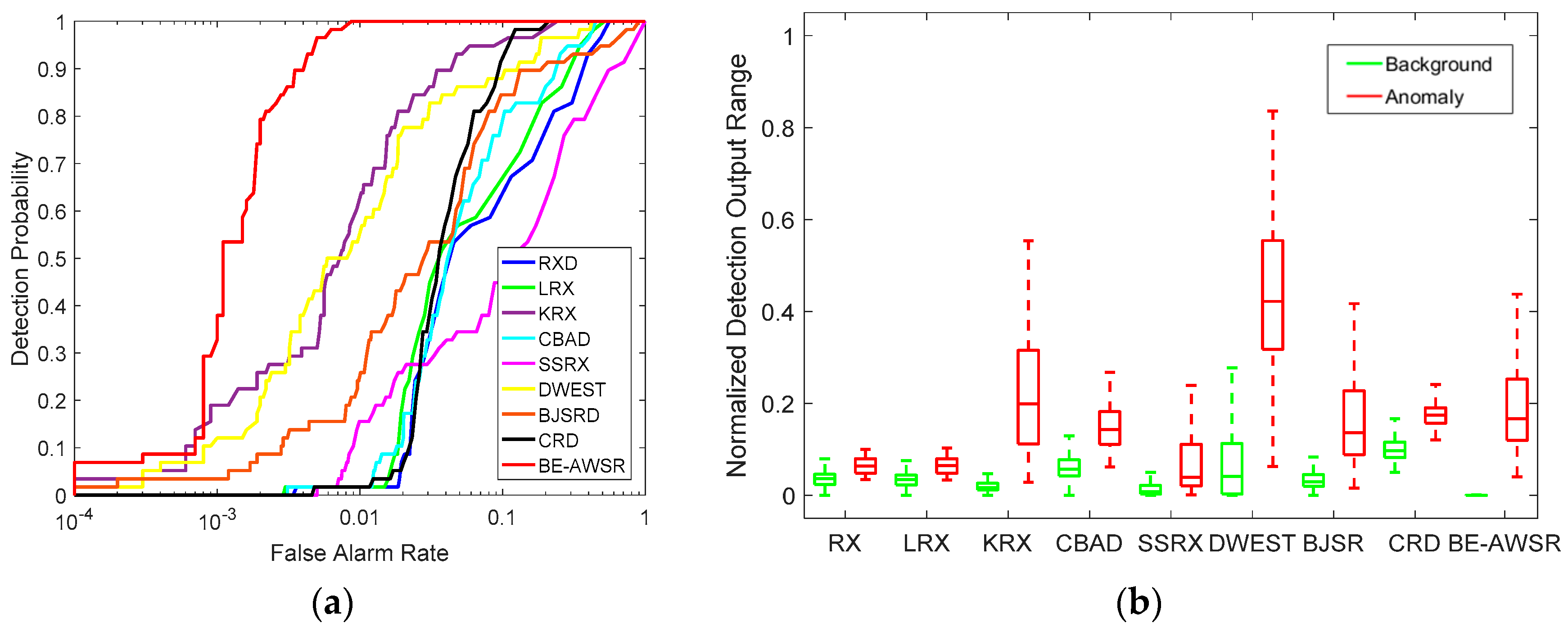
In this subsection, the detection performance is evaluated quantitatively by receiver operating characteristic (ROC) curves [41] and the normalized background-anomaly separation maps. Based on the ground truth, the ROC curve plots the relationship between the detection rate DR and the false alarm rate FAR; DR and FAR are defined as follows:
where Ndetection is the number of correctly-detected anomaly pixels and Nanomaly is the total number of anomaly pixels in the image. Nfalse is the number of falsely-detected anomaly pixels and Nimage is the total number of pixels in the image. The ROC curve of an outstanding detector is located near the top left of the coordinate plane, since it can achieve a high detection rate with a low false alarm rate. Moreover, the AUC value is also used to measure the detection performance, which denotes the area under the ROC curve. A detector with better detection performance has a larger AUC value.
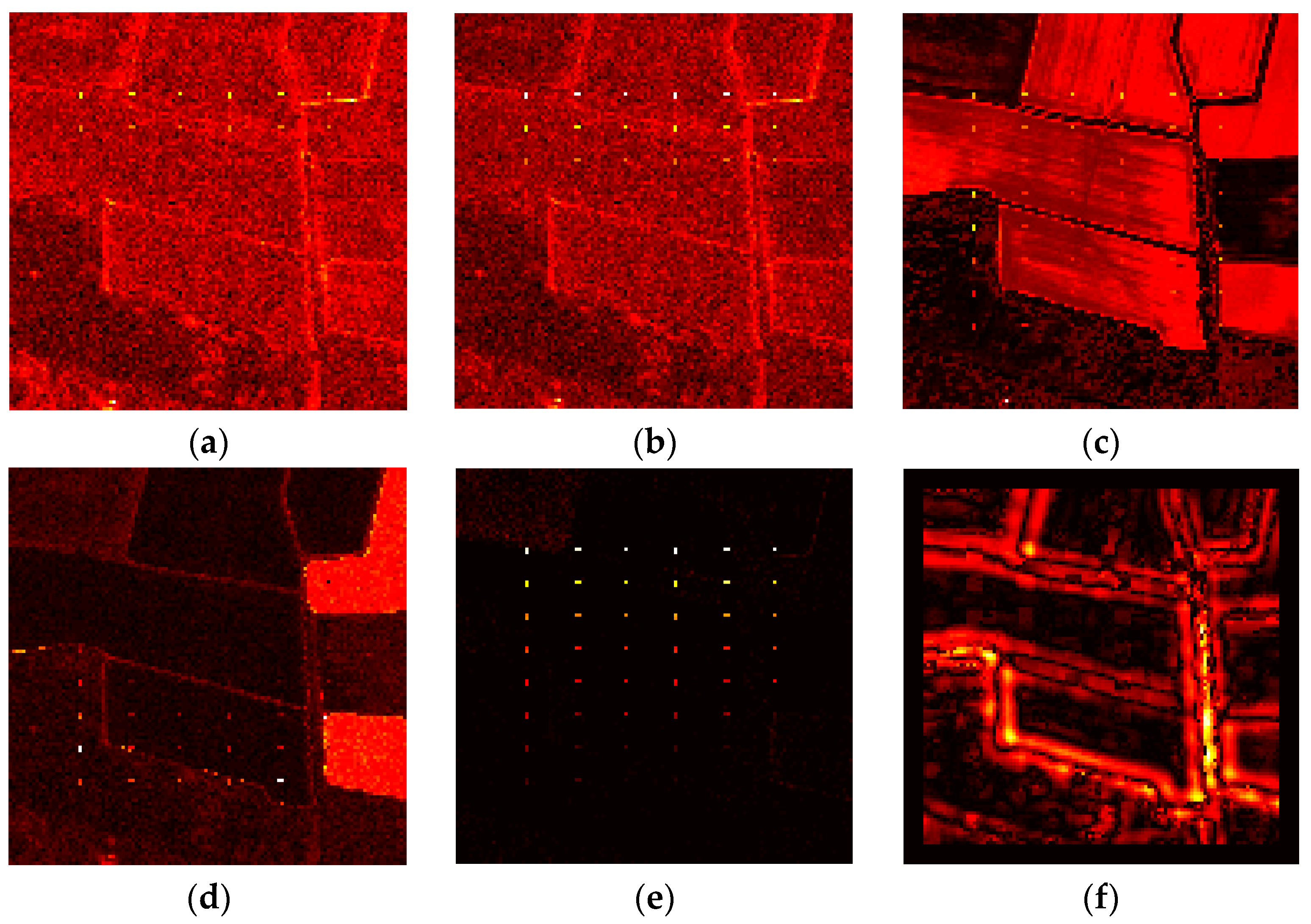
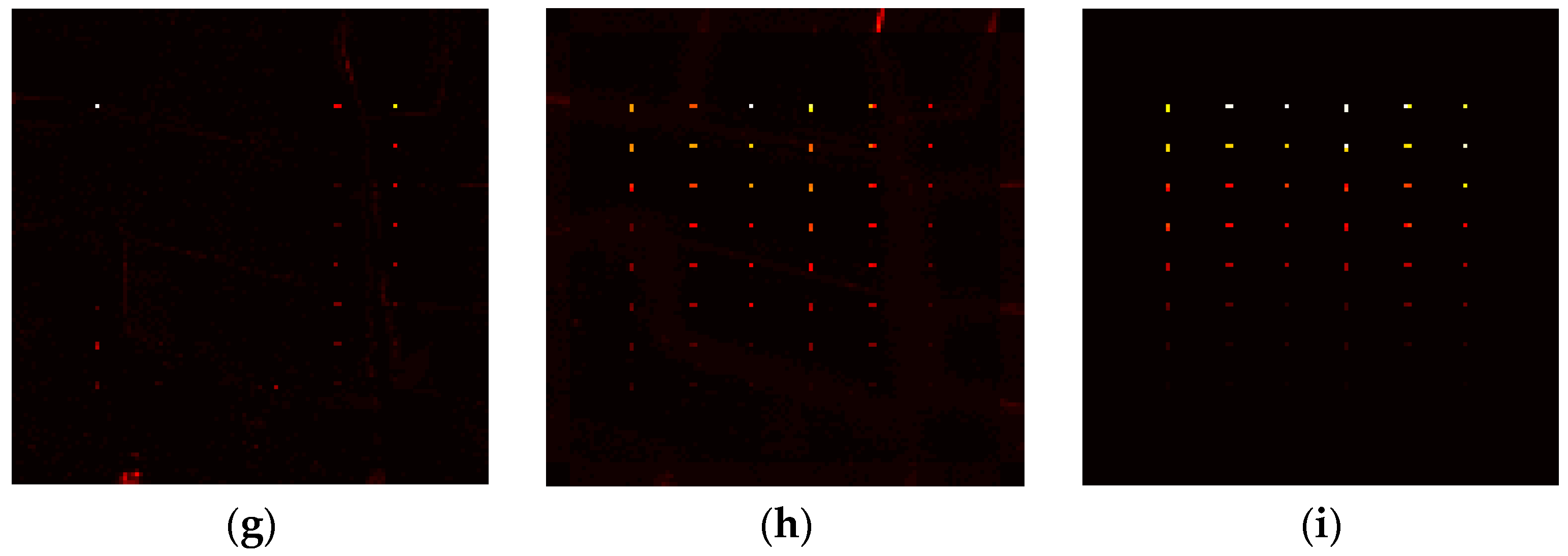
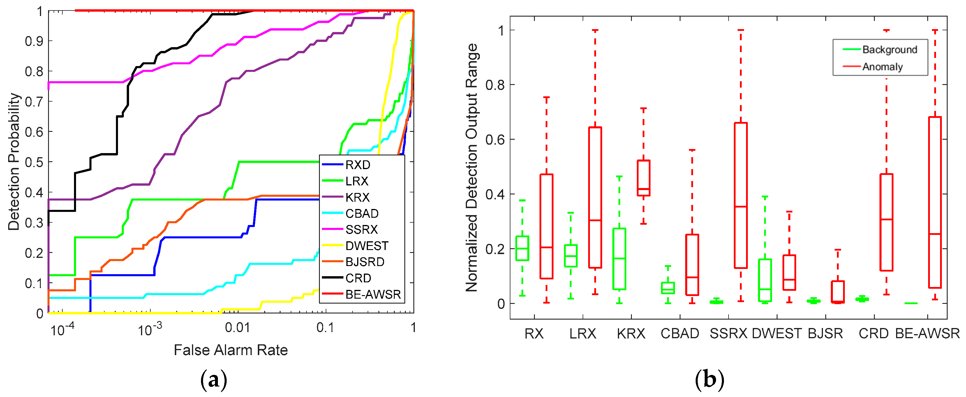
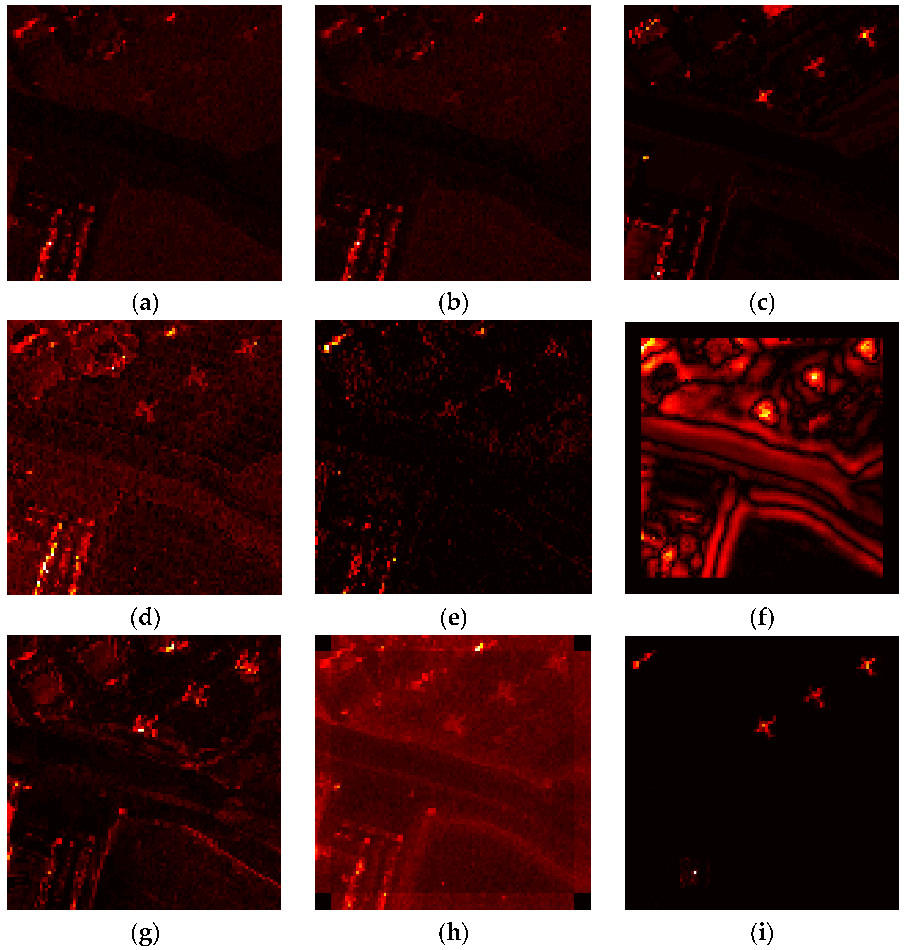
For the Hyperion dataset, the color detection maps of algorithms in comparison are shown in Figure 7. As shown in Figure 7, SSRX and CRD obtain a superior performance in background suppression and anomaly extraction overall. However, for SSRX, the suppression of the background in the top left and bottom right of the scene is relatively weak, which can increase the false alarm rate. For CRD, an obvious false alarm exists in the top right of the scene. In addition, RX and LRX have a poor background suppression, and only anomaly targets with high anomaly abundance fractions can be well detected. For KRX, the background suppression is also not very effective, but the detection performance is better than RX and LRX. Some anomaly targets with low anomaly abundance fractions are still distinguishable. For CBAD, most of the background can be suppressed. However, there are two backgrounds in the right of the scene that are bright, which can influence the detection result. In DWEST, serious false alarms occur in the edges of backgrounds and in roads, and the anomaly targets are not distinguishable. BJSRD can well suppress the background, but the performance of extract anomalies is not satisfactory, since many anomaly targets are missed in the map. For the proposed BE-AWSR algorithm, it can be seen that the background suppression performance is outstanding, and meanwhile, all anomaly targets are successfully extracted. A quantitative analysis of these different anomaly detection algorithms for the Hyperion dataset is illustrated in Figure 8. Figure 8a presents the ROC curves of each algorithm. It can be observed that the BE-AWSR algorithm achieves a perfect detection performance, since the 100% detection rate can be obtained when the false alarm rate is nearly equal to zero. SSRX, KRX and CRD also have a relatively higher detection rate when the false alarm rate is low. Except for SSRX, KRX, CRD and the BE-AWSR algorithm, the other compared algorithms’ ROC curves are away from the top left corner, which indicates that they cannot detect all anomaly targets in a reasonable false alarm rate. Figure 8b demonstrates the separability of background and anomaly targets in all investigated algorithms through the background-anomaly separation map. For the convenience of comparison, values of all detection results are normalized to 0–1. Each detector has two boxes: the green one represents the distributions of background pixels’ values, and the red one is the distributions of anomaly pixels’ values. The central mark in each box indicates the median, while the bottom and top edges indicate the lower quartile and the upper quartile, with the whiskers indicate the extreme values within 1.5-times the interquartile range from the end of the box. From Figure 8b, it is proven that the BE-AWSR algorithm can suppress the background information to a small range, and the gap between the anomaly box and the background box is large when compared with the other detectors. Therefore, the BE-AWSR algorithm has the best background-anomaly separation performance in all compared algorithms.
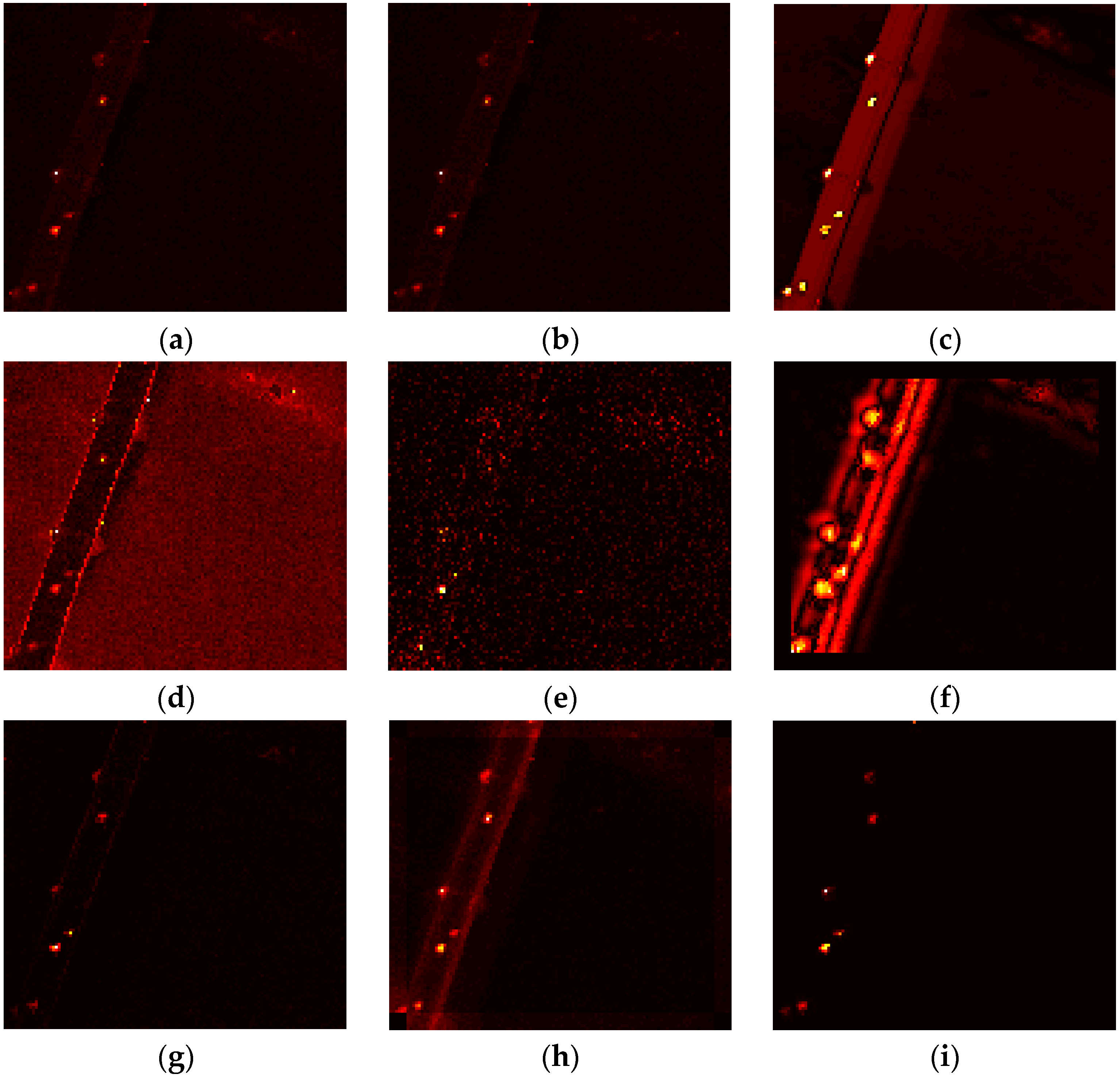
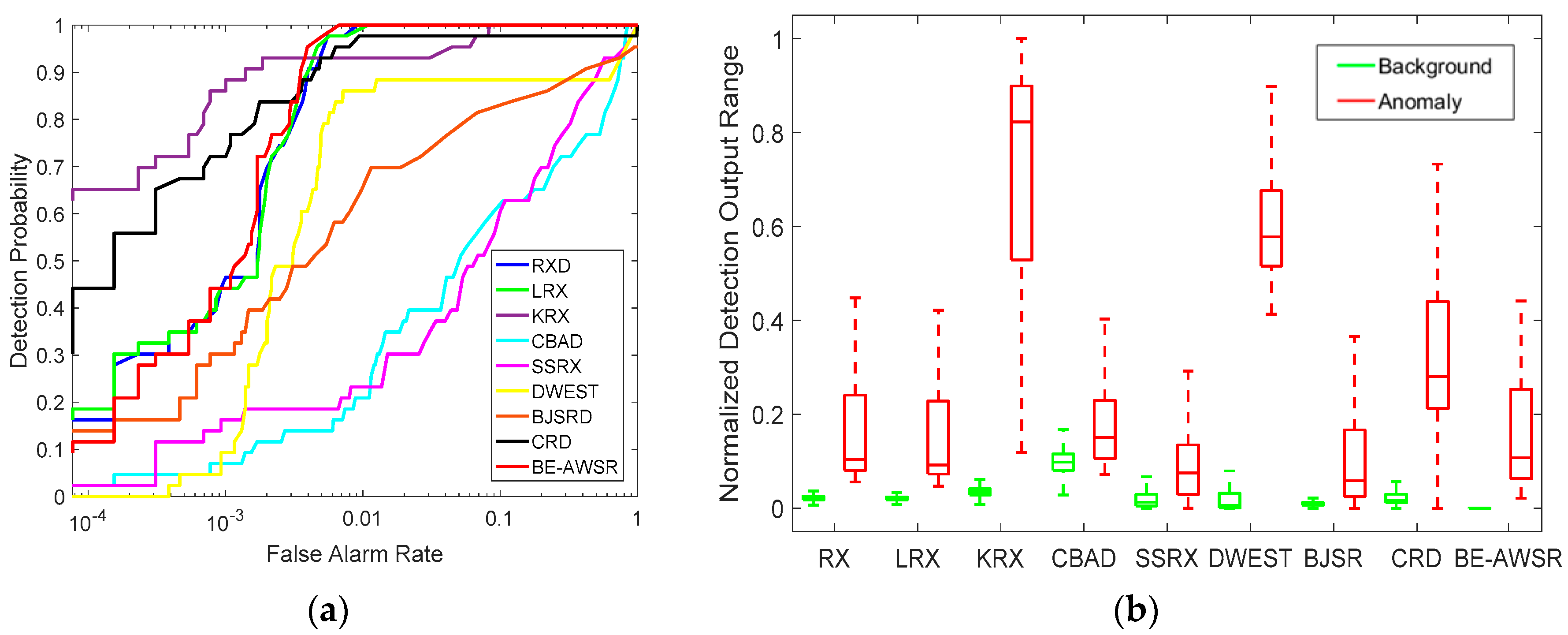
For the ROSIS dataset, the color detection maps of all compared algorithms are illustrated in Figure 9. It can be seen that RX, LRX, BJSRD and the BE-AWSR algorithm have relatively better performance in background suppression, and among them, the BE-AWSR algorithm is the best. Apart from this, the anomaly targets extraction of these four algorithms are all effective. Moreover, in CBAD, the suppression for the background of water is not satisfactory, and the separation of background and anomaly targets is not obvious enough. In SSRX, the performance of anomaly target extraction is poor, and a part of the anomalies is indistinguishable from the background. For DWEST, it can suppress the background of water successfully, but the suppression for the background of the bridge is relatively bad; on the other hand, it performs well in anomaly target extraction. For KRX and CRD, they achieve a remarkable performance in both background suppression and anomaly target extraction. Figure 10 shows the quantitative comparisons of these algorithms for the ROSIS dataset via ROC curves and background-anomaly separation map. From Figure 10a, it can be seen that RX, LRX and the BE-AWSR algorithm obtain superior ROC curves, and a 100% detection rate can be achieved when the false alarm rate is at a lower level. KRX and CRD have very high detection rates when the false alarm rate is less than 0.001, but the false alarms are relatively serious when they obtain a 100% detection rate. In contrast, the ROC curves of DWEST, BJSRD, CBAD and SSRX are relatively worse. Moreover, as shown in Figure 10b, the BE-AWSR algorithm can separate background and anomaly targets effectively, and the background information can be enclosed in a very small range when compared with the other algorithms.
For the AVIRIS dataset, Figure 11 shows the color detection maps of all compared algorithms. It can be observed from Figure 11 that RX and LRX nearly fail to extract the anomaly targets, and the result of SSRX is a little better. In CBAD, the anomaly targets are more distinguishable than the three previously-mentioned algorithms, but the background suppression is not very satisfactory. In DWEST, the anomaly targets can be well extracted, but the false alarms are relatively serious. In comparison, KRX, BJSRD and CRD have better detection performances. For the BE-AWSR algorithm, the performance of background suppression is the best, and meanwhile, anomaly targets can be extracted accurately and clearly. Furthermore, the quantitative comparisons of these algorithms for the AVIRIS dataset are depicted in Figure 12. The ROC curves of all compared algorithms are presented in Figure 12a. It can be seen from Figure 12a that the BE-AWSR algorithm has a significantly better ROC curve than the others. In the BE-AWSR algorithm, all anomaly pixels can be detected with the false alarm rate less than 0.01. In addition, the background-anomaly separation map is demonstrated in Figure 12b. It shows that the BE-AWSR algorithm has a more advanced performance when compared with the other algorithms.
Then, the AUC values of each compared algorithm for three datasets are listed in Table 1, and the highest AUC value of each dataset is displayed in bold. The statistics in Table 1 further indicate that the BE-AWSR algorithm yields the best detection performance in all the compared algorithms. In fact, three datasets in our experiments have different characteristics. For the Hyperion dataset, anomaly targets have different abundance fractions. Some algorithms may miss anomalies with lower abundance fractions, such as RX and LRX. Some algorithms cannot effectively detect anomalies located in some specific types of backgrounds, such as CBAD and BJSRD. For the ROSIS dataset, the background compositions are relatively simple, and nearly all algorithms have reasonable detection performances. For the AVIRIS dataset, it contains several different types of backgrounds, which can make the detection more difficult. However, the BE-AWSR algorithm achieves very high AUC values (more than 0.99) for all datasets, which proves the robustness of the proposed algorithm. Furthermore, the computing time of each compared algorithm for three datasets is reported in Table 2. It can be seen from Table 2 that the BE-AWSR algorithm is more efficient than DWEST and BJSRD and slightly better than CRD. In a word, the computational cost of the BE-AWSR algorithm can stay in a reasonable range.
4.3 Parameter Analysis
In this subsection, we evaluate the influences of the different parameters settings on the detection performances of the BE-AWSR algorithm. There are five important parameters in our proposed method: (1) the VEP’s lower bound L0; (2) the suspected anomaly center’s lower bound L1; (3) the structure element’s (SE) size W × W; (4) the expansion coefficient λ; and (5) the sparsity level K0. For simplicity, the shape of SE is set as square, and the background dictionary DB is generated by collecting 1/3 of the pixels in the background elements set HB randomly. In addition, the detection performances under any parameter combinations are evaluated by AUC values, and the other parameters are fixed as the corresponding optimal while analyzing the specific parameter (s).
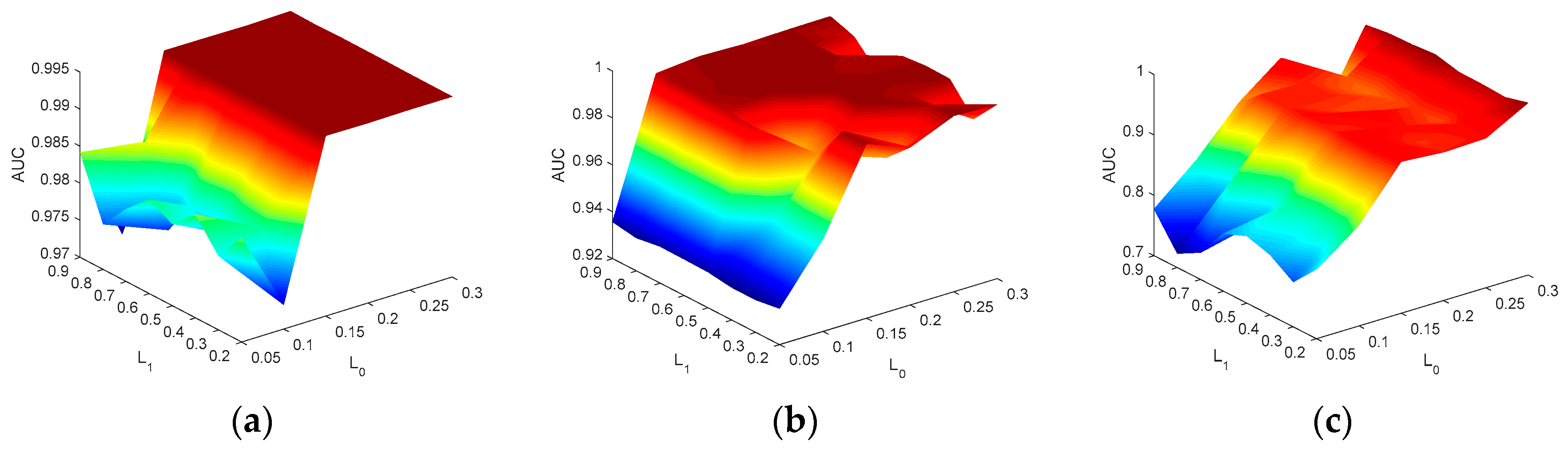
We first analyze the influence of VEP’s lower bound L0 and the suspected anomaly center’s lower bound L1 on the Hyperion, ROSIS and AVIRIS datasets. The three dimensional (3D) plots are used to display the detection performance simultaneously, which is shown in Figure 13. The L0 is changed from 0.05–0.3, while the L1 is changed from 0.2–0.9 on each dataset. From Figure 13, it can be seen that with the increasing of L0 in the range from 0.05–0.15, the detection performance has a significant improvement on each dataset. When L0 is in the range of 0.15–0.3, the BE-AWSR algorithm can obtain satisfactory detection results, confirmed by AUC values that are larger than 0.9 for all datasets. Therefore, it is reasonable to determine that the VEP’s lower bound L0 is not less than 0.15. In addition, it can be seen from Figure 13 that the change of L1 does not cause an obvious effect to the detection performance. It reflects that the BE-AWSR algorithm is not very sensitive to the transformation of L1. Thus, Figure 13 exhibits that if L0 is set in a suitable range, then the BE-AWSR algorithm can obtain a reasonable and stable detection performance, which proves the robustness of the BE-AWSR algorithm to this parameters set.
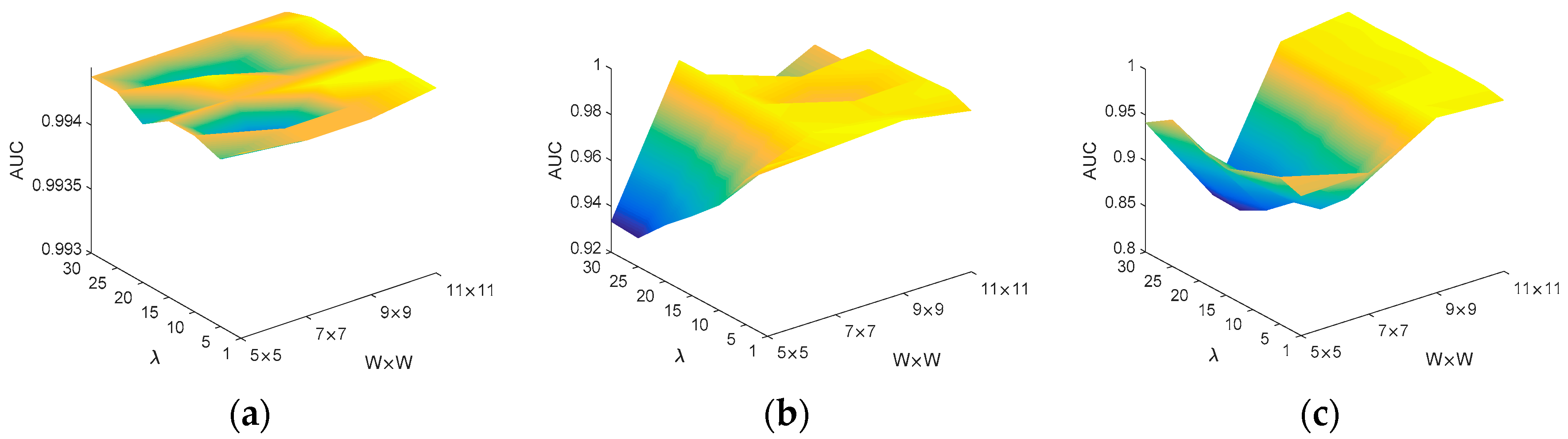
Then, we investigate the sensitiveness of the BE-AWSR algorithm to the SE’s size W × W and the expansion coefficient λ on the Hyperion, ROSIS and AVIRIS datasets. The 3D plot of the detection performance is depicted in Figure 14. The range of the size W × W is set from 5 × 5–11 × 11, and λ is varied from 1–30 for all datasets. From Figure 14a, it can be seen that the BE-AWSR algorithm has a superior and stable detection performance for the Hyperion dataset; because the AUC surface is relatively flat and lies at a high position, which is above higher than 0.994. From Figure 14b, it can be seen that the BE-AWSR algorithm achieves a satisfactory detection performance when the size W × W is 7 × 7. If the size is too large or too small, the detection performance is decreased with the increase of expansion coefficient λ. This is apparent since the estimation of suspected anomaly pixels will not be accurate enough if the size has a large bias for the true size of anomalies. This phenomenon also occurs in Figure 14c, but in this subfigure, if the size W × W is large than 9 × 9, the detection performance is relatively satisfactory and stable. This is because the anomaly sizes in the AVIRIS dataset are relatively large. From Figure 14, it can be concluded that in the BE-AWSR algorithm, the SE’s size W × W is an essential parameter, which needs to be identified in a certain range, while the algorithm is not very sensitive to the expansion coefficient λ relatively.
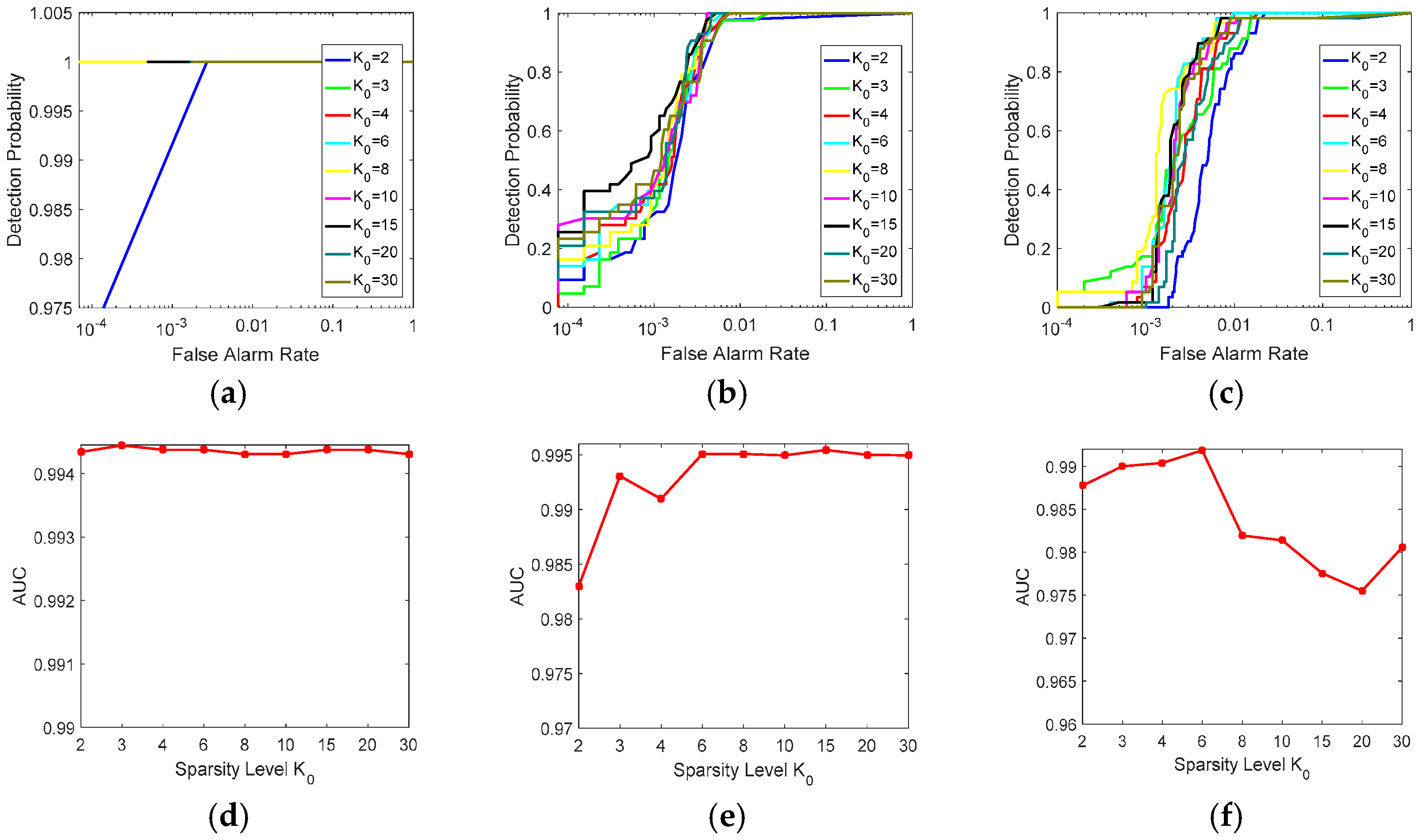
Finally the sparsity level K0 is discussed on the Hyperion, ROSIS and AVIRIS datasets. Its upper bound is set as K0 = 2,3,4,6,8,10,15,20,30 for all datasets, and the detection performances are displayed by the two dimensional (2D) plots, as shown in Figure 15. Figure 15a–c illustrates the ROC curves under different sparsity levels for each dataset, and Figure 15d–f depicts the corresponding AUC curves. It can be seen from Figure 15 that the BE-AWSR algorithm is not sensitive to the change of sparsity level K0 in a wide and reasonable range; since the AUC curves lie in a high position of the AUC-axis (above higher than 0.95) for all datasets. In detail, for the Hyperion dataset in Figure 15a,d, when K0 is larger than two, a 100% detection rate can be achieved with a very low false alarm rate. In addition, the AUC values are very high and stable with the variation of K0. These two subfigures indicate that for the Hyperion dataset, K0 almost has no effect on the detection performance of the BE-AWSR algorithm. From Figure 15b and Figure 15e, it can be seen that for the ROSIS dataset, the detection performance of the BE-AWSR algorithm improves gradually with K0 increasing from 2 –6, and then, the AUC curve tends to be stable relatively. The best detection performance is achieved when K0 is equal to 15. For the AVIRIS dataset in Figure 15c,f, the detection performance of the BE-AWSR algorithm improves slowly when K0 is from 2–6, and it has a decrease as K0 continues to increase. When K0 is equal to six, the BE-AWSR algorithm has the best performance.
From the aforementioned analyses, the VEP’s lower bound L0 and SE’s size W × W are two parameters in the BE-AWSR algorithm that have a relatively obvious influence on the detection performance. The first one needs to be determined empirically based on the endmembers’ abundance image set, and the second one is related to the sizes of anomalies in the dataset. In addition, the BE-AWSR algorithm is relatively insensitive to the suspected anomaly center’s lower bound L1, the expansion coefficient λ and the sparsity level K0. On the whole, the BE-AWSR algorithm is quite robust to the settings of parameters if they are in reasonable ranges.
5. Conclusions
In this paper, a novel hyperspectral anomaly detection algorithm via background estimation and adaptive weighted sparse representation is proposed. To obtain the dictionary that contains background information and without the contamination of anomalies, a new background dictionary construction method is provided. Furthermore, the sparse representation adaptively weighted on both global and local domains is used in the proposed method. In this way, the discrimination between anomalies and background is enhanced. The metric to determine anomalies is based on the residual calculated in the algorithm. Extensive experiments on both synthetic and real HSI datasets confirm that the proposed anomaly detection algorithm has superior detection performance compared to the other detection methods. Moreover, the parameter sensitivity analysis proves the robustness of the proposed method with reasonable parameters settings.
Author Contributions
Lingxiao Zhu proposed the general idea of the method and performed the experiments. Gongjian Wen provided many constructive advices for the preparation. This paper was written by Lingxiao Zhu.
Conflicts of Interest
The authors declare no conflict of interest.
References
- Bioucas-Dias, J.M.; Plaza, A.; Camps-Valls, G.; Scheunders, P.; Nasrabadi, N.; Chanussot, J. Hyperspectral remote sensing data analysis and future challenges. IEEE Geosci. Remote Sens. Mag. 2013, 1, 6–36. [Google Scholar] [CrossRef]
- Shaw, G.; Manolakis, D. Signal processing for hyperspectral image exploitation. IEEE Signal Process. Mag. 2002, 19, 12–16. [Google Scholar] [CrossRef]
- Manolakis, D.G. Overview of algorithms for hyperspectral target detection—Theory and practice. In Proceedings of the SPIE, Orlando, FL, USA, 30 July 2002; pp. 202–215. [Google Scholar]
- Manolakis, D.; Lockwood, R.; Cooley, T.; Jacobson, J. Is There a Best Hyperspectral Detection Algorithm? The International Society for Optical Engineering: Bellingham, WA, USA, 2009. [Google Scholar]
- Chang, C.-I.; Chiang, S.-S. Anomaly detection and classification for hyperspectral imagery. IEEE Trans. Geosci. Remote Sens. 2002, 40, 1314–1325. [Google Scholar] [CrossRef]
- Stefanou, M.S.; Kerekes, J.P. Image-derived prediction of spectral image utility for target detection applications. IEEE Trans. Geosci. Remote Sens. 2010, 48, 1827–1833. [Google Scholar] [CrossRef]
- Manolakis, D.; Shaw, G. Detection algorithms for hyperspectral imaging applications. IEEE Signal Process. Mag. 2002, 19, 29–43. [Google Scholar] [CrossRef]
- Stein, D.W.; Beaven, S.G.; Hoff, L.E.; Winter, E.M.; Schaum, A.P.; Stocker, A.D. Anomaly detection from hyperspectral imagery. IEEE Signal Process. Mag. 2002, 19, 58–69. [Google Scholar] [CrossRef]
- Eismann, M.T.; Stocker, A.D.; Nasrabadi, N.M. Automated hyperspectral cueing for civilian search and rescue. Proc. IEEE 2009, 97, 1031–1055. [Google Scholar] [CrossRef]
- Reed, I.S.; Yu, X. Adaptive multiple-band cfar detection of an optical pattern with unknown spectral distribution. IEEE Trans. Acoust. Speech Signal Process. 1990, 38, 1760–1770. [Google Scholar] [CrossRef]
- Carlotto, M.J. A cluster-based approach for detecting man-made objects and changes in imagery. IEEE Trans. Geosci. Remote Sens. 2005, 43, 374–387. [Google Scholar] [CrossRef]
- Schaum, A. Joint subspace detection of hyperspectral targets. In Proceedings of the 2004 IEEE Aerospace Conference, Big Sky, MT, USA, 6–13 March 2004; IEEE: Piscataway, NJ, USA, 2004. [Google Scholar]
- Qu, Y.; Qi, H.; Ayhan, B.; Kwan, C.; Kidd, R. Does multispectral/hyperspectral pansharpening improve the performance of anomaly detection? In Proceedings of the IEEE International Geoscience and Remote Sensing Symposium (IGARSS), Fort Worth, TX, USA, 23–28 July 2017; pp. 6130–6133. [Google Scholar]
- Kwon, H.; Nasrabadi, N.M. Kernel rx-algorithm: A nonlinear anomaly detector for hyperspectral imagery. IEEE Trans. Geosci. Remote Sens. 2005, 43, 388–397. [Google Scholar] [CrossRef]
- Zhou, J.; Kwan, C.; Ayhan, B.; Eismann, M.T. A novel cluster kernel RX algorithm for anomaly and change detection using hyperspectral images. IEEE Trans. Geosci. Remote Sens. 2016, 54, 6497–6504. [Google Scholar] [CrossRef]
- Schaum, A. Advanced hyperspectral detection based on elliptically contoured distribution models and operator feedback. In Proceedings of the 2009 IEEE Applied Imagery Pattern Recognition Workshop (AIPRW), Washington, DC, USA, 14–16 October 2009; IEEE: Piscataway, NJ, USA, 2009; pp. 1–5. [Google Scholar]
- Du, B.; Zhang, L. Random-selection-based anomaly detector for hyperspectral imagery. IEEE Trans. Geosci. Remote Sens. 2011, 49, 1578–1589. [Google Scholar] [CrossRef]
- Zhao, R.; Du, B.; Zhang, L. A robust nonlinear hyperspectral anomaly detection approach. IEEE J. Sel. Top. Appl. Earth Obs. Remote Sens. 2014, 7, 1227–1234. [Google Scholar] [CrossRef]
- Billor, N.; Hadi, A.S.; Velleman, P.F. Bacon: Blocked adaptive computationally efficient outlier nominators. Comput. Stat. Data Anal. 2000, 34, 279–298. [Google Scholar] [CrossRef]
- Du, B.; Zhang, L. A discriminative metric learning based anomaly detection method. IEEE Trans. Geosci. Remote Sens. 2014, 52, 6844–6857. [Google Scholar]
- Kwon, H.; Der, S.Z.; Nasrabadi, N.M. Adaptive anomaly detection using subspace separation for hyperspectral imagery. Opt. Eng. 2003, 42, 3342–3351. [Google Scholar] [CrossRef]
- Liu, W.-m.; Chang, C.-I. Multiple-window anomaly detection for hyperspectral imagery. IEEE J. Sel. Top. Appl. Earth Obs. Remote Sens. 2013, 6, 644–658. [Google Scholar] [CrossRef]
- Li, W.; Du, Q. Collaborative representation for hyperspectral anomaly detection. IEEE Trans. Geosci. Remote Sens. 2015, 53, 1463–1474. [Google Scholar] [CrossRef]
- Li, J.; Zhang, H.; Zhang, L.; Ma, L. Hyperspectral anomaly detection by the use of background joint sparse representation. IEEE J. Sel. Top. Appl. Earth Obs. Remote Sens. 2015, 8, 2523–2533. [Google Scholar] [CrossRef]
- Dao, M.; Kwan, C.; Ayhan, B.; Tran, T.D. Burn scar detection using cloudy modis images via low-rank and sparsity-based models. In Proceedings of the 2016 IEEE Global Conference on Signal and Information Processing (GlobalSIP), Washington, DC, USA, 7–9 December 2016; IEEE: Piscataway, NJ, USA; pp. 177–181. [Google Scholar]
- Dao, M.; Kwan, C.; Koperski, K.; Marchisio, G. A joint sparsity approach to tunnel activity monitoring using high resolution satellite images. In Proceedings of the IEEE Ubiquitous Computing, Electronics and Mobile Communication Conference, New York, NY, USA, 19–21 October 2017. [Google Scholar]
- Xu, Y.; Wu, Z.; Li, J.; Plaza, A.; Wei, Z. Anomaly detection in hyperspectral images based on low-rank and sparse representation. IEEE Trans. Geosci. Remote Sens. 2016, 54, 1990–2000. [Google Scholar] [CrossRef]
- Niu, Y.; Wang, B. Hyperspectral target detection using learned dictionary. IEEE Geosci. Remote Sens. Lett. 2015, 12, 1531–1535. [Google Scholar]
- Gruninger, J.; Ratkowski, A.J.; Hoke, M.L. The Sequential Maximum Angle Convex Cone (SMACC) Endmember Model; Spectral Sciences Inc.: Burlington, MA, USA, 2004. [Google Scholar]
- Chen, Y.; Nasrabadi, N.M.; Tran, T.D. Hyperspectral image classification using dictionary-based sparse representation. IEEE Trans. Geosci. Remote Sens. 2011, 49, 3973–3985. [Google Scholar] [CrossRef]
- Chen, Y.; Nasrabadi, N.M.; Tran, T.D. Sparse representation for target detection in hyperspectral imagery. IEEE J. Sel. Top. Signal Process. 2011, 5, 629–640. [Google Scholar] [CrossRef]
- Tropp, J.A.; Wright, S.J. Computational methods for sparse solution of linear inverse problems. Proc. IEEE 2010, 98, 948–958. [Google Scholar] [CrossRef]
- Mallat, S.G.; Zhang, Z. Matching pursuits with time-frequency dictionaries. IEEE Trans. Signal Process. 1993, 41, 3397–3415. [Google Scholar] [CrossRef]
- Tropp, J.A.; Gilbert, A.C. Signal recovery from random measurements via orthogonal matching pursuit. IEEE Trans. Inf. Theory 2007, 53, 4655–4666. [Google Scholar] [CrossRef]
- Luo, B.; Chanussot, J.; Douté, S.; Zhang, L. Empirical automatic estimation of the number of endmembers in hyperspectral images. IEEE Geosci. Remote Sens. Lett. 2013, 10, 24–28. [Google Scholar]
- Zhang, Y.; Du, B.; Zhang, L. A sparse representation-based binary hypothesis model for target detection in hyperspectral images. IEEE Trans. Geosci. Remote Sens. 2015, 53, 1346–1354. [Google Scholar] [CrossRef]
- Borghys, D.; Kåsen, I.; Achard, V.; Perneel, C. Comparative evaluation of hyperspectral anomaly detectors in different types of background. In Proceedings of the Algorithms and Technologies for Multispectral, Hyperspectral, and Ultraspectral Imagery XVIII, Baltimore, MD, USA, 24 May 2012; International Society for Optics and Photonics: Bellingham, WA, USA, 2012; p. 83902J. [Google Scholar]
- Schweizer, S.M.; Moura, J.M. Efficient detection in hyperspectral imagery. IEEE Trans. Image Process. 2001, 10, 584–597. [Google Scholar] [CrossRef] [PubMed]
- Khazai, S.; Homayouni, S.; Safari, A.; Mojaradi, B. Anomaly detection in hyperspectral images based on an adaptive support vector method. IEEE Geosci. Remote Sens. Lett. 2011, 8, 646–650. [Google Scholar] [CrossRef]
- Stefanou, M.S.; Kerekes, J.P. A method for assessing spectral image utility. IEEE Trans. Geosci. Remote Sens. 2009, 47, 1698–1706. [Google Scholar] [CrossRef]
- Kerekes, J. Receiver operating characteristic curve confidence intervals and regions. IEEE Geosci. Remote Sens. Lett. 2008, 5, 251–255. [Google Scholar] [CrossRef]
Figure 1.
Illustration of the extraction result of the sequential maximum angle convex cone (SMACC) endmember model. The first row is the abundance image of each endmember; the lighter pixels have higher abundance fractions of this endmember; while the corresponding endmember spectrum is shown in the second row.

Figure 2.
Different cases in the structure element’s (SE) sliding process. Regions in gold denote valid endmember pixels (VEPs) and in white invalid endmember pixels (IEPs). (a) All pixels in SE are VEPs; (b) a part of the pixels in SE are VEPs, the others are IEPs; (c) pixels in a striped area in SE are VEPs, the others are IEPs; (d) pixels in a tiny area in the center of SE are VEPs, the others are IEPs.

Figure 3.
Schematic illustration of the proposed anomaly detection method.

Figure 4.
Hyperion dataset for experiment. (a) Image scene with implanted targets; (b) locations, sizes and abundance fractions of implanted targets; (c) spectra of anomaly and main backgrounds (B).
Figure 4.
Hyperion dataset for experiment. (a) Image scene with implanted targets; (b) locations, sizes and abundance fractions of implanted targets; (c) spectra of anomaly and main backgrounds (B).

Figure 5.
Reflective Optics Spectrographic Imaging System (ROSIS) dataset for the experiment. (a) Image scene of Pavia city; (b) distributions of anomaly pixels; (c) spectra of anomaly and main backgrounds.
Figure 5.
Reflective Optics Spectrographic Imaging System (ROSIS) dataset for the experiment. (a) Image scene of Pavia city; (b) distributions of anomaly pixels; (c) spectra of anomaly and main backgrounds.

Figure 6.
AVIRIS dataset for the experiment. (a) Image scene of San Diego; (b) distributions of anomaly pixels; (c) spectra of anomaly and main backgrounds.
Figure 6.
AVIRIS dataset for the experiment. (a) Image scene of San Diego; (b) distributions of anomaly pixels; (c) spectra of anomaly and main backgrounds.

Figure 7.
Color detection maps of different algorithms for the Hyperion dataset. (a) Reed–Xiaoli detector (RX); (b) local RX (LRX); (c) kernel-RX (KRX); (d) cluster-based anomaly detection (CBAD); (e) subspace RX (SSRX); (f) dual window-based Eigen separation transform (DWEST); (g) background joint sparse representation detector (BJSRD); (h) collaborative representation-based detector (CRD); (i) background estimation and adaptive weighted sparse representation algorithm (BE-AWSR).


Figure 8.
Quantitative analysis of compared algorithms for the Hyperion dataset. (a) ROC curves; (b) background-anomaly separation map.
Figure 8.
Quantitative analysis of compared algorithms for the Hyperion dataset. (a) ROC curves; (b) background-anomaly separation map.

Figure 9.
Color detection maps of different algorithms for the ROSIS dataset. (a) RX; (b) LRX; (c) KRX; (d) CBAD; (e) SSRX; (f) DWEST; (g) BJSRD; (h) CRD; (i) BE-AWSR.
Figure 9.
Color detection maps of different algorithms for the ROSIS dataset. (a) RX; (b) LRX; (c) KRX; (d) CBAD; (e) SSRX; (f) DWEST; (g) BJSRD; (h) CRD; (i) BE-AWSR.

Figure 10.
Quantitative analysis of compared algorithms for the ROSIS dataset. (a) ROC curves; (b) background-anomaly separation map.
Figure 10.
Quantitative analysis of compared algorithms for the ROSIS dataset. (a) ROC curves; (b) background-anomaly separation map.

Figure 11.
Color detection maps of different algorithms for the AVIRIS dataset. (a) RX; (b) LRX; (c) KRX; (d) CBAD; (e) SSRX; (f) DWEST; (g) BJSRD; (h) CRD; (i) BE-AWSR.
Figure 11.
Color detection maps of different algorithms for the AVIRIS dataset. (a) RX; (b) LRX; (c) KRX; (d) CBAD; (e) SSRX; (f) DWEST; (g) BJSRD; (h) CRD; (i) BE-AWSR.

Figure 12.
Quantitative analysis of compared algorithms for the AVIRIS dataset. (a) ROC curves; (b) background-anomaly separation map.
Figure 12.
Quantitative analysis of compared algorithms for the AVIRIS dataset. (a) ROC curves; (b) background-anomaly separation map.

Figure 13.
AUC illustration for different settings of the VEP’s lower bound L0 and the suspected anomaly center’s lower bound L1 on three HSI datasets. (a) Hyperion dataset; (b) ROSIS dataset; (c) AVIRIS dataset.
Figure 13.
AUC illustration for different settings of the VEP’s lower bound L0 and the suspected anomaly center’s lower bound L1 on three HSI datasets. (a) Hyperion dataset; (b) ROSIS dataset; (c) AVIRIS dataset.

Figure 14.
AUC illustration for different settings of the SE’s size W × W and the expansion coefficient λ on three HSI datasets. (a) Hyperion dataset; (b) ROSIS dataset; (c) AVIRIS dataset.
Figure 14.
AUC illustration for different settings of the SE’s size W × W and the expansion coefficient λ on three HSI datasets. (a) Hyperion dataset; (b) ROSIS dataset; (c) AVIRIS dataset.

Figure 15.
Illustration for different settings of the sparsity level K0 on three HSI datasets. (a,d) ROC curves and AUC curve for the Hyperion dataset; (b,e) ROC curves and AUC curve for the ROSIS dataset; (c,f) ROC curves and AUC curve for the AVIRIS dataset.
Figure 15.
Illustration for different settings of the sparsity level K0 on three HSI datasets. (a,d) ROC curves and AUC curve for the Hyperion dataset; (b,e) ROC curves and AUC curve for the ROSIS dataset; (c,f) ROC curves and AUC curve for the AVIRIS dataset.


Table 1.
AUC values of different algorithms for the Hyperion, ROSIS and AVIRIS datasets.
| AUC | RX | LRX | KRX | CBAD | SSRX | DWEST | BJSRD | CRD | BE-AWSR |
|---|---|---|---|---|---|---|---|---|---|
| Hyperion | 0.5079 | 0.6676 | 0.9642 | 0.5744 | 0.9853 | 0.6176 | 0.4998 | 0.9936 | 0.9944 |
| ROSIS | 0.9949 | 0.9949 | 0.9922 | 0.7803 | 0.8184 | 0.8998 | 0.8894 | 0.9727 | 0.9952 |
| AVIRIS | 0.8688 | 0.8938 | 0.9753 | 0.9103 | 0.7815 | 0.9584 | 0.9092 | 0.9469 | 0.9924 |
Table 2.
Computing time of different algorithms for the Hyperion, ROSIS and AVIRIS datasets.
| Time (s) | RX | LRX | KRX | CBAD | SSRX | DWEST | BJSRD | CRD | BE-AWSR |
|---|---|---|---|---|---|---|---|---|---|
| Hyperion | 0.659 | 64.474 | 13.006 | 1.543 | 0.571 | 209.355 | 3905.349 | 118.397 | 109.352 |
| ROSIS | 0.154 | 45.955 | 6.780 | 0.762 | 0.293 | 125.091 | 2679.727 | 47.380 | 74.940 |
| AVIRIS | 0.175 | 45.217 | 2.319 | 0.578 | 0.181 | 141.988 | 2016.940 | 81.305 | 56.397 |
© 2018 by the authors. Licensee MDPI, Basel, Switzerland. This article is an open access article distributed under the terms and conditions of the Creative Commons Attribution (CC BY) license (http://creativecommons.org/licenses/by/4.0/).
Share and Cite
MDPI and ACS Style
Zhu, L.; Wen, G. Hyperspectral Anomaly Detection via Background Estimation and Adaptive Weighted Sparse Representation. Remote Sens. 2018, 10, 272. https://0-doi-org.brum.beds.ac.uk/10.3390/rs10020272
AMA Style
Zhu L, Wen G. Hyperspectral Anomaly Detection via Background Estimation and Adaptive Weighted Sparse Representation. Remote Sensing. 2018; 10(2):272. https://0-doi-org.brum.beds.ac.uk/10.3390/rs10020272
Chicago/Turabian StyleZhu, Lingxiao, and Gongjian Wen. 2018. "Hyperspectral Anomaly Detection via Background Estimation and Adaptive Weighted Sparse Representation" Remote Sensing 10, no. 2: 272. https://0-doi-org.brum.beds.ac.uk/10.3390/rs10020272
Note that from the first issue of 2016, this journal uses article numbers instead of page numbers. See further details here.