Simulation and Analysis of the Topographic Effects on Snow-Free Albedo over Rugged Terrain

 , , ,
, , ,
Abstract
:
1. Introduction
2. Methods
2.1. BSA over a Rugged Terrain
2.2. BSA Estimation Method Derivation
2.3. Topographic Effect Analysis Methods
3. Datasets
3.1. Simulated DEM Dataset
3.2. Global Digital Elevation Model (GDEM)
3.3. Reference BSA Dataset Simulation Based on the Radiative Approach
4. Results and Discussion
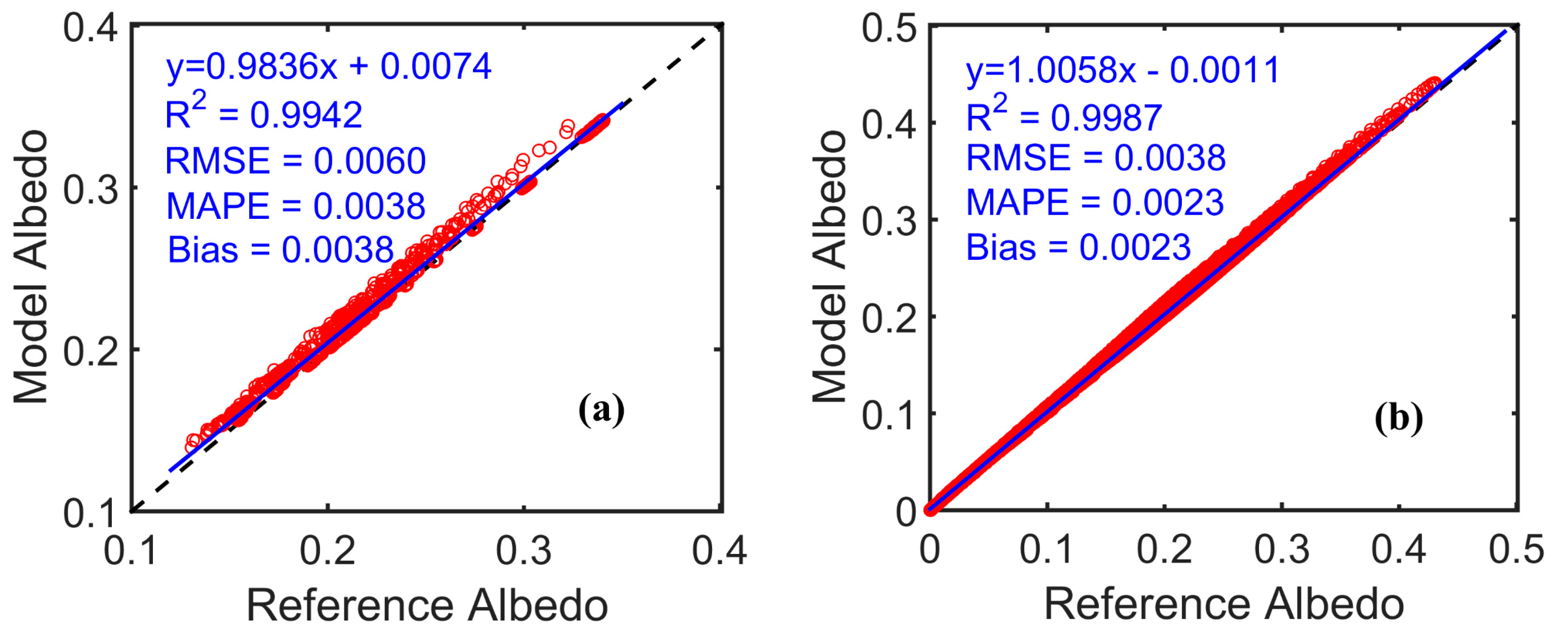
4.1. Modeled BSA Accuracy Assessment
4.2. Topographic Effects on BSA
4.2.1. Factors Influencing the BSA over a Rugged Terrain
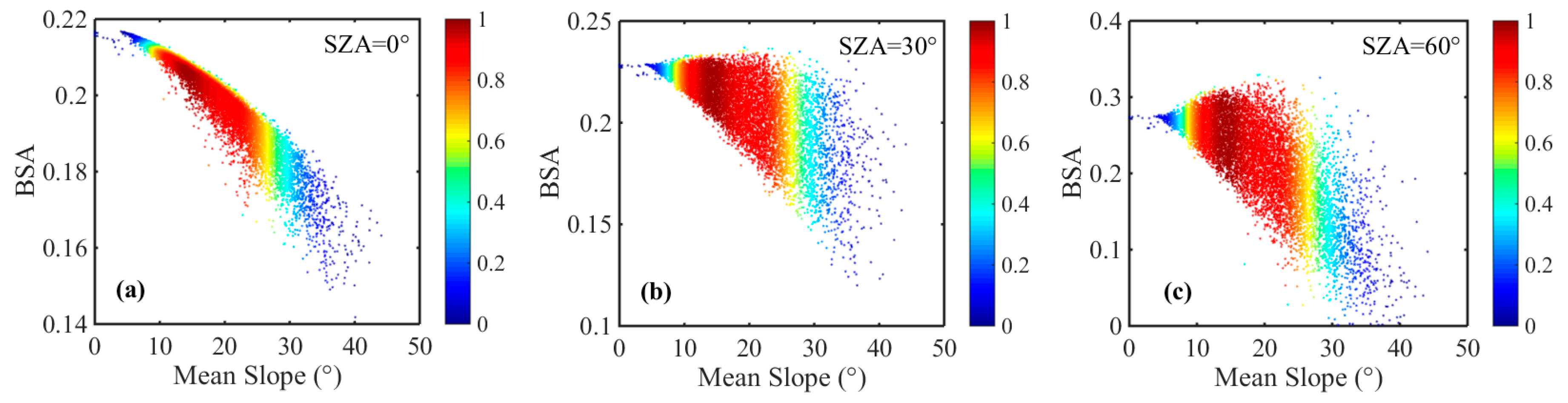
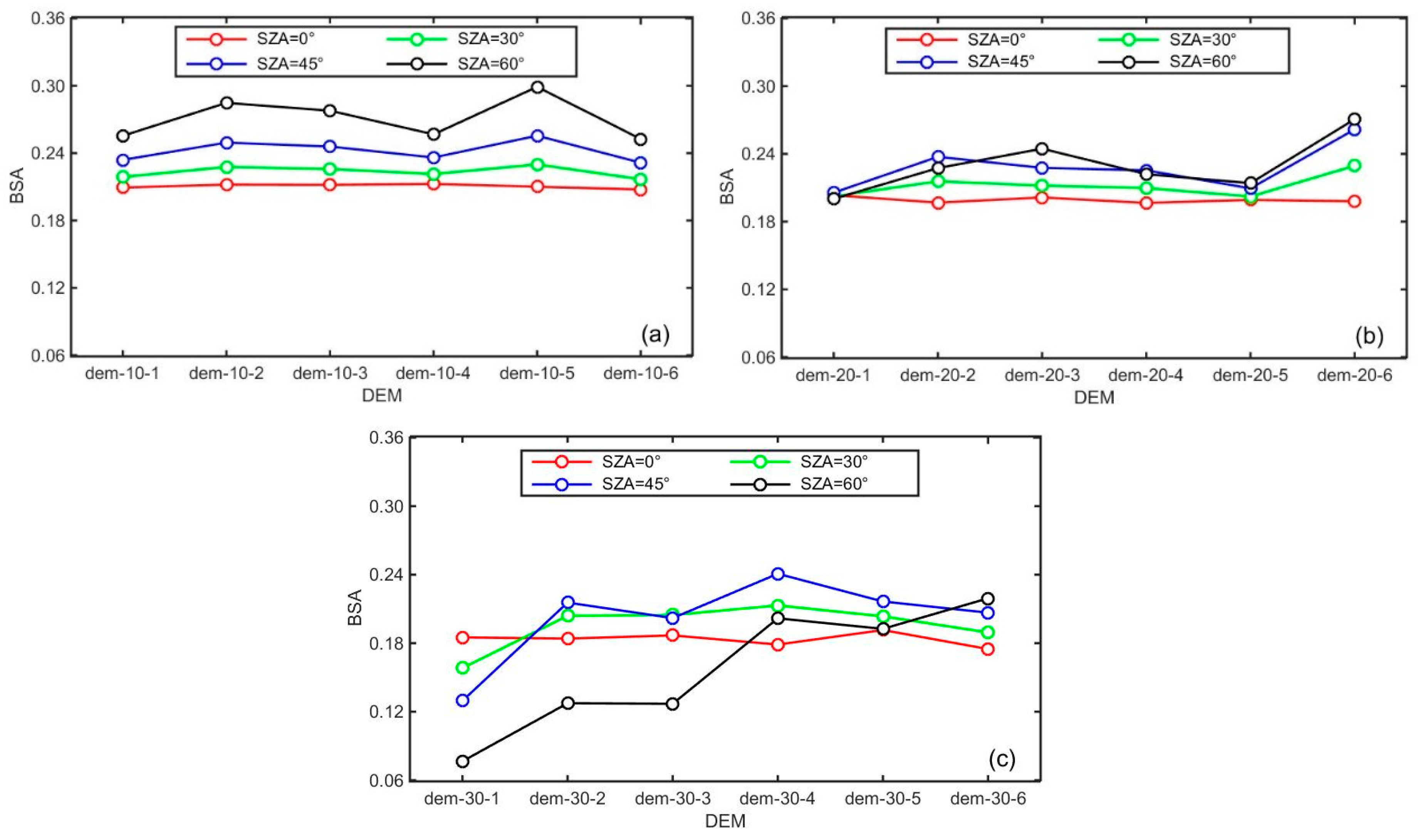
4.2.2. BSA Variation with Mean Slope
4.2.3. BSA Variations with Sub-Pixel Aspect Distributions
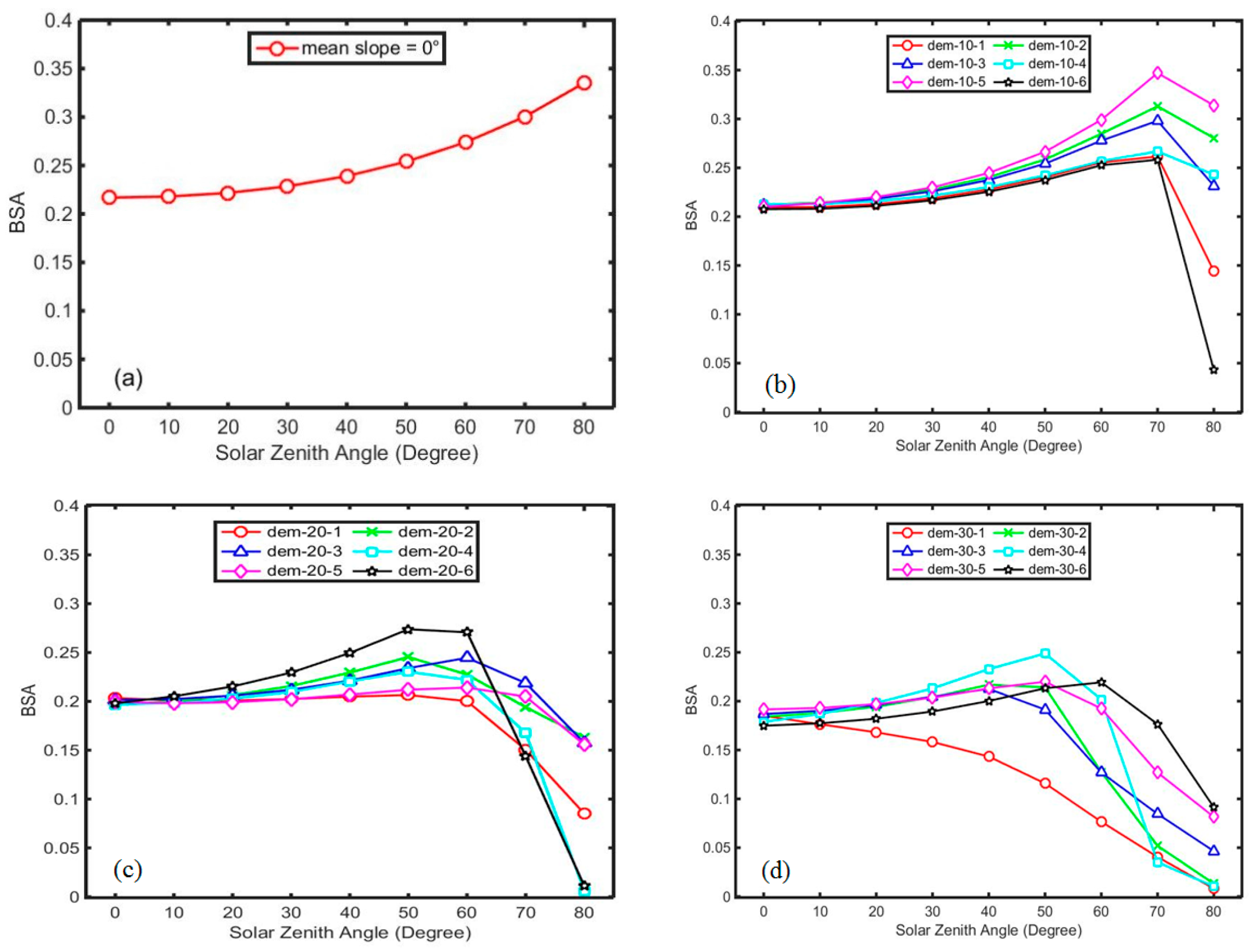
4.2.4. BSA Variation with SZA
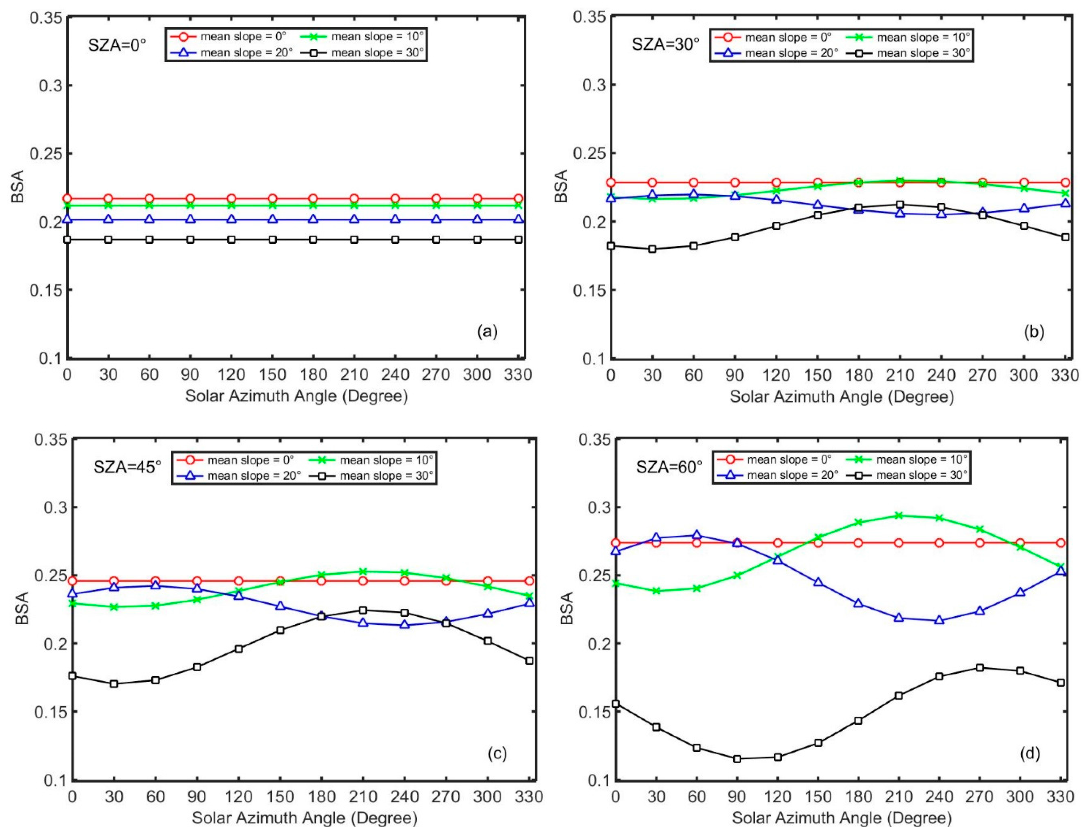
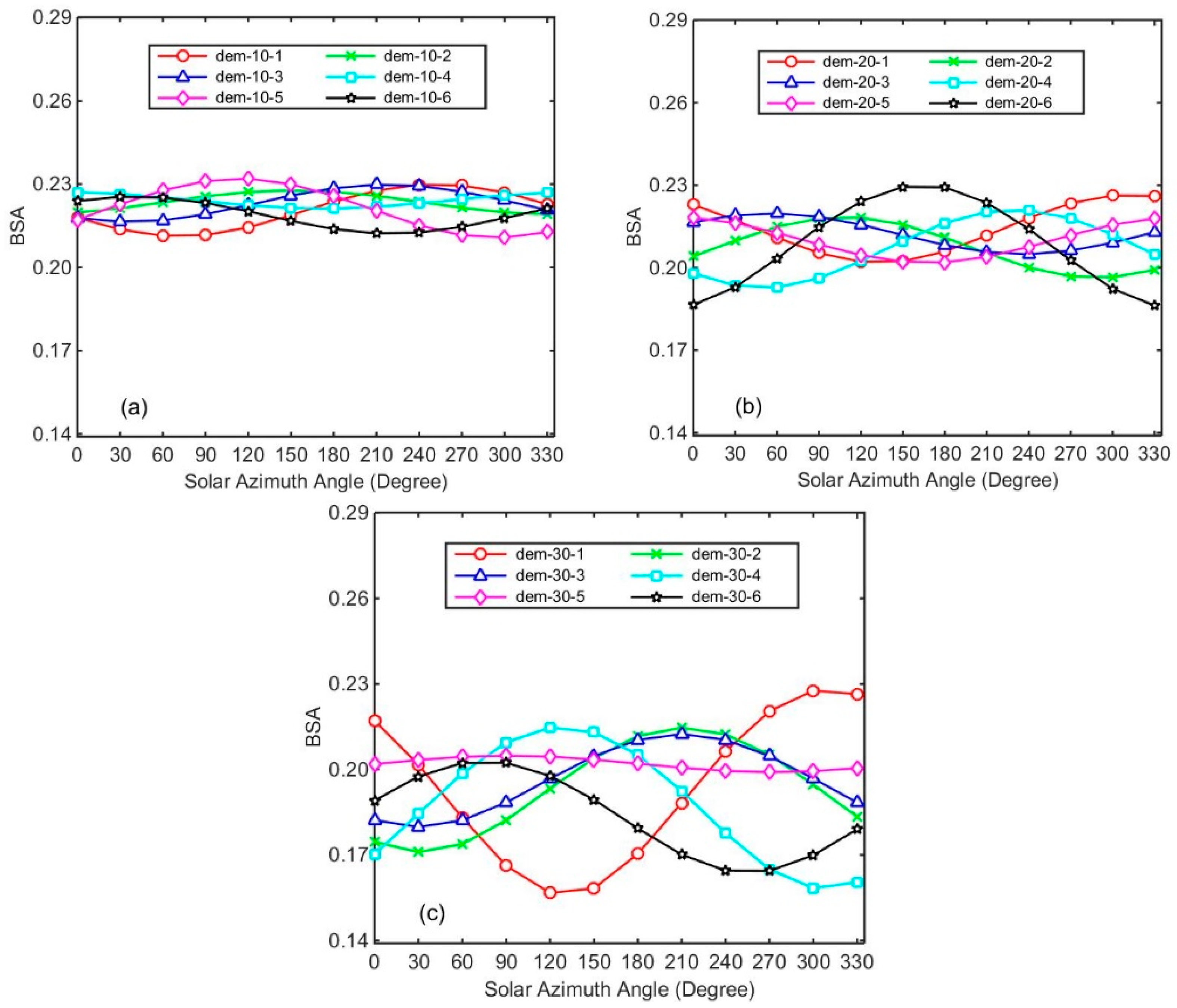
4.2.5. BSA Variation with SAA
4.3. Method Limitations
5. Conclusions
Acknowledgments
Author Contributions
Conflicts of Interest
References
- Liang, S. Quantitative Remote Sensing of Land Surfaces; Wiley-Interscience: Hoboken, NJ, USA, 2003; pp. 413–415. [Google Scholar]
- Qu, Y.; Liang, S.; Liu, Q.; He, T.; Liu, S.; Li, X. Mapping surface broadband albedo from satellite observations: A review of literatures on algorithms and products. Remote Sens. 2015, 7, 990–1020. [Google Scholar] [CrossRef]
- Martonchik, J.V.; Bruegge, C.J.; Strahler, A.H. A review of reflectance nomenclature used in remote sensing. Remote Sens. Rev. 2000, 19, 9–20. [Google Scholar] [CrossRef]
- Schaepman-Strub, G.; Schaepman, M.E.; Painter, T.H.; Dangel, S.; Martonchik, J.V. Reflectance quantities in optical remote sensing—Definitions and case studies. Remote Sens. Environ. 2006, 103, 27–42. [Google Scholar] [CrossRef]
- Schaepman-Strub, G.; Schaepman, M.E.; Martonchik, J.V.; Painter, T.H.; Dangel, S. Radiometry and reflectance: From terminology concepts to measured quantities. In The SAGE Handbook of Remote Sensing; Sage Publications: Thousand Oaks, CA, USA, 2009. [Google Scholar]
- Lucht, W.; Schaaf, C.B.; Strahler, A.H. An algorithm for the retrieval of albedo from space using semiempirical BRDF models. IEEE Trans. Geosci. Remote Sens. 2002, 38, 977–998. [Google Scholar] [CrossRef]
- Combal, B.; Isaka, H.; Trotter, C. Extending a turbid medium BRDF model to allow sloping terrain with a vertical plant stand. IEEE Trans. Geosci. Remote Sens. 2000, 38, 798–810. [Google Scholar] [CrossRef]
- Schaaf, C.; Li, X.; Strahler, A. Topographic effects on bidirectional and hemispherical reflectances calculated with a geometric-optical canopy model. IEEE Trans. Geosci. Remote Sens. 1994, 32, 1186–1193. [Google Scholar] [CrossRef]
- Strahler, A.H.; Muller, J.; Lucht, W.; Schaaf, C.; Tsang, T.; Gao, F.; Li, X.; Lewis, P.; Barnsley, M.J. MODIS BRDF/Albedo Product: Algorithm Theoretical Basis Document. Version 5.0. Available online: https://modis.gsfc.nasa.gov/data/atbd/atbd_mod09.pdf (accessed on 1 October 2017).
- Liang, S. A direct algorithm for estimating land surface broadband albedos from MODIS imagery. IEEE Trans. Geosci. Remote Sens. 2003, 41, 136–145. [Google Scholar] [CrossRef]
- Tasumi, M.; Allen, R.G.; Trezza, R. At-surface reflectance and albedo from satellite for operational calculation of land surface energy balance. J. Hydrol. Eng. 2008, 13, 51–63. [Google Scholar] [CrossRef]
- Schaaf, C.B.; Gao, F.; Strahler, A.H.; Lucht, W.; Li, X.; Schaaf, C.B.; Gao, F.; Strahler, A.H.; Lucht, W.; Li, X. First Operational BRDF, Albedo Nadir Reflectance Products from MODIS. Remote Sens. Environ. 2002, 83, 135–148. [Google Scholar] [CrossRef]
- Deschamps, P.Y.; Breon, F.M.; Leroy, M.; Podaire, A.; Bricaud, A.; Buriez, J.C.; Seze, G. The polder mission: Instrument characteristics and scientific objectives. IEEE Trans. Geosci. Remote Sens. 1994, 32, 598–615. [Google Scholar] [CrossRef]
- Diner, D.J.; Beckert, J.C.; Reilly, T.H.; Bruegge, C.J.; Conel, J.E.; Kahn, R.A.; Martonchik, J.V.; Ackerman, T.P.; Davies, R.; Gerstl, S.A.W. Multi-angle imaging spectroradiometer (MISR) instrument description and experiment overview. IEEE Trans. Geosci. Remote Sens. 2005, 36, 1072–1087. [Google Scholar] [CrossRef]
- Rutan, D.; Charlock, T.P.; Rose, F.; Kato, S.; Zentz, S.; Coleman, L. Global Surface Albedo from Ceres/Terra Surface and Atmospheric Radiation Budget (SARB) Data Product; ACM: New York City, NY, USA, 2006; pp. 2245–2255. [Google Scholar]
- Ryu, Y.; Kang, S.; Moon, S.K.; Kim, J. Evaluation of land surface radiation balance derived from moderate resolution imaging spectroradiometer (MODIS) over complex terrain and heterogeneous landscape on clear sky days. Agric. For. Meteorol. 2008, 148, 1538–1552. [Google Scholar] [CrossRef]
- Wen, J.; Zhao, X.; Liu, Q.; Tang, Y.; Dou, B. An improved land-surface albedo algorithm with DEM in rugged terrain. IEEE Geosci. Remote Sens. Lett. 2014, 11, 883–887. [Google Scholar]
- Gao, B.; Jia, L.; Menenti, M. An improved method for retrieving land surface albedo over rugged terrain. IEEE Geosci. Remote Sens. Lett. 2014, 11, 554–558. [Google Scholar] [CrossRef]
- Wen, J.G.; Qiang, L.; Liu, Q.H.; Xiao, Q.; Li, X.W. Scale effect and scale correction of land-surface albedo in rugged terrain. Int. J. Remote Sens. 2009, 30, 5397–5420. [Google Scholar] [CrossRef]
- Fan, W.; Chen, J.M.; Ju, W.; Zhu, G. GOST: A geometric-optical model for sloping terrains. IEEE Trans. Geosci. Remote Sens. 2014, 52, 5469–5482. [Google Scholar]
- Mousivand, A.; Verhoef, W.; Menenti, M.; Gorte, B. Modeling top of atmosphere radiance over heterogeneous non-lambertian rugged terrain. Remote Sens. 2015, 7, 8019–8044. [Google Scholar] [CrossRef]
- Yin, G.; Li, A.; Zhao, W.; Jin, H.; Bian, J.; Wu, S. Modeling canopy reflectance over sloping terrain based on path length correction. IEEE Trans. Geosci. Remote Sens. 2017, 55, 4597–4609. [Google Scholar] [CrossRef]
- Manninen, T.; Andersson, K.; Riihelä, A. Topography Correction of the CM-SAF Surface Albedo Product SAL. In Proceedings of the EUMETSAT Meteorological Satellite Conference, Oslo, Norway, 5–9 September 2011. [Google Scholar]
- Kawata, Y.; Ueno, S.; Kusaka, T. Radiometric correction for atmospheric and topographic effects on landsat mss images. Remote Sens. 1988, 9, 729–748. [Google Scholar] [CrossRef]
- Li, H.; Shen, Y.; Yang, P.; Zhao, W.; Allen, R.G.; Shao, H.; Lei, Y. Calculation of albedo on complex terrain using MODIS data: A case study in Taihang mountain of China. Environ. Earth Sci. 2015, 74, 1–10. [Google Scholar] [CrossRef]
- Cherubini, F.; Vezhapparambu, S.; Bogren, W.; Astrup, R.; Strømman, A.H. Spatial, seasonal, and topographical patterns of surface albedo in Norwegian forests and cropland. Int. J. Remote Sens. 2017, 38, 4565–4586. [Google Scholar] [CrossRef]
- Ashdown, I. Radiosity: A Programmer’s Perspective; John Wiley & Sons, Inc.: Hoboken, NJ, USA, 1994; pp. 7–10. [Google Scholar]
- Proy, C.; Tanre, D.; Deschamps, P.Y. Evaluation of topographic effects in remotely sensed data. Remote Sens. Environ. 1989, 30, 21–32. [Google Scholar] [CrossRef]
- Chen, Y.; Hall, A.; Liou, K.N. Application of three-dimensional solar radiative transfer to mountains. J. Geophys. Res. Atmos. 2006, 111, 5143–5162. [Google Scholar] [CrossRef]
- Richter, R.; Schläpfer, D. Geo-atmospheric processing of airborne imaging spectrometry data. Part 2: Atmospheric/topographic correction. Int. J. Remote Sens. 2002, 23, 2631–2649. [Google Scholar] [CrossRef]
- Sandmeier, S.; Itten, K.I. A physically-based model to correct atmospheric and illumination effects in optical satellite data of rugged terrain. IEEE Trans. Geosci. Remote Sens. 1997, 35, 708–717. [Google Scholar] [CrossRef]
- Dozier, J.; Frew, J. Rapid calculation of terrain parameters for radiation modeling from digital elevation data. IEEE Trans. Geosci. Remote Sens. 1990, 28, 963–969. [Google Scholar] [CrossRef]
- Zaksek, K.; Ostir, K.; Kokalj, Z. Sky-view factor as a relief visualization technique. Remote Sens. 2011, 3, 398–415. [Google Scholar] [CrossRef]
- Hapke, B. Theory of Reflectance and Emittance Spectroscopy: Second Edition; Cambridge University Press: Cambridge, UK, 2012; pp. 303–335. [Google Scholar]
- Hapke, B. Bidirectional reflectance spectroscopy: 3. Correction for macroscopic roughness. Icarus 1984, 59, 41–59. [Google Scholar] [CrossRef]
- Jacquemoud, S.; Verhoef, W.; Baret, F.; Bacour, C.; Zarcotejada, P.J.; Asner, G.P.; François, C.; Ustin, S.L.; Ustin, S.L.; Schaepman, M.E. Prospect+sail models: A review of use for vegetation characterization. Remote Sens. Environ. 2009, 113, S56–S66. [Google Scholar] [CrossRef]
- Cariboni, J.; Gatelli, D.; Liska, R.; Saltelli, A. The role of sensitivity analysis in ecological modelling. Ecol. Model. 2007, 203, 167–182. [Google Scholar] [CrossRef]
- Roupioz, L.; Nerry, F.; Jia, L.; Menenti, M. Improved surface reflectance from remote sensing data with sub-pixel topographic information. Remote Sens. 2014, 6, 10356–10374. [Google Scholar] [CrossRef]
- Liang, S.; Lewis, P.; Dubayah, R.; Qin, W.; Shirey, D. Topographic effects on surface bidirectional reflectance scaling. J. Remote Sens. 1997, 1, 82–93. [Google Scholar]
- Borel, C.C.; Gerstl, S.A.W.; Powers, B.J. The radiosity method in optical remote sensing of structured 3-d surfaces. Remote Sens. Environ. 1991, 36, 13–44. [Google Scholar]
- Goel, N.S.; Rozehnal, I.; Thompson, R.L. A computer graphics-based model for scattering from objects of arbitrary shapes in the optical region. Remote Sens. Environ. 1991, 36, 73–104. [Google Scholar] [CrossRef]
- Wang, K.; Wang, P.; Liu, J.; Sparrow, M.; Haginoya, S.; Zhou, X. Variation of surface albedo and soil thermal parameters with soil moisture content at a semi-desert site on the western Tibetan plateau. Bound. Layer Meteorol. 2005, 116, 117–129. [Google Scholar] [CrossRef]
- Oguntunde, P.G.; Ajayi, A.E.; Giesen, N.V.D. Tillage and surface moisture effects on bare-soil albedo of a tropical loamy sand. Soil Tillage Res. 2006, 85, 107–114. [Google Scholar] [CrossRef]
- Pinty, B.; Verstraete, M.M.; Dickinson, R.E. A physical model for predicting bidirectional reflectances over bare soil. Remote Sens. Environ. 1989, 27, 273–288. [Google Scholar] [CrossRef]
- Pinker, R.T.; Laszlo, I. Modeling surface solar irradiance for satellite applications on a global scale. J. Appl. Meteorol. 1992, 31, 194–211. [Google Scholar] [CrossRef]
- Sirguey, P. Simple correction of multiple reflection effects in rugged terrain. Int. J. Remote Sens. 2009, 30, 1075–1081. [Google Scholar]


| Filter | Exaggeration | Mean Elevation (m) | Mean Slope (°) | Mean Sky View Factor |
|---|---|---|---|---|
| 5 × 1 | 1 | 29.49 | 1.33 | 1.00 |
| 3 × 1 | 1 | 29.49 | 1.88 | 1.00 |
| 1 × 1 | 1 | 29.49 | 2.51 | 1.00 |
| 5 × 1 | 10 | 294.89 | 12.84 | 0.95 |
| 3 × 1 | 10 | 294.89 | 17.59 | 0.90 |
| 1 × 1 | 10 | 294.89 | 22.62 | 0.85 |
| 5 × 1 | 20 | 589.78 | 23.70 | 0.83 |
| 3 × 1 | 20 | 589.78 | 30.90 | 0.74 |
| 1 × 1 | 20 | 589.78 | 37.72 | 0.64 |
| Model Parameters | Unit | Range | |
|---|---|---|---|
| Leaf parameters | Leaf structure index | unitless | 1.5 |
| Leaf chlorophyll content | [μg/cm2] | 40 | |
| Leaf dry matter content | [g/cm2] | 0.009 | |
| Leaf water content | [cm] | 0.01 | |
| Leaf brown pigment | [g/cm2] | 0.0 | |
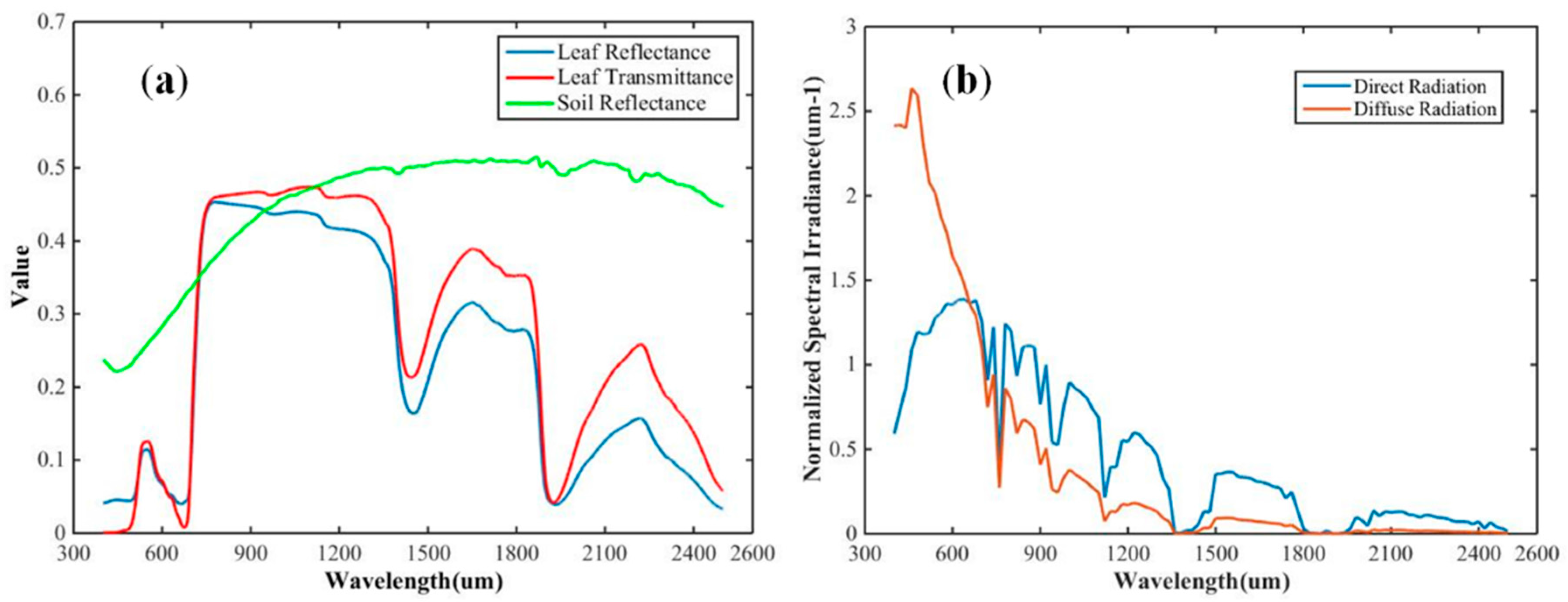
| Soil parameters | Reflectance | ------ | Shown in Figure 4a |
| Canopy structure parameters | LAI | [m2/m2] | 3 |
| Leaf inclination distribution function | ------ | Spherical | |
| Hot spot size parameter | [m/m] | 0.01 | |
| Atmospheric condition | Incoming radiation | ------ | Shown in Figure 4b |
| Illumination view geometry | Solar zenith angle | [°] | 0–90 at a 5° interval |
| Solar azimuth angle | [°] | 0–360 at a 5° interval | |
| View zenith angle | [°] | 0–90 at a 5° interval | |
| View azimuth angle | [°] | 0–360 at a 5° interval | |
| Terrain | DEM | ------ | Nine simulated DEMs and real DEMs |
| Mean Slope (°) | R2 | RMSE | MAPE | Bias |
|---|---|---|---|---|
| 1.33 | 1.0000 | 0.0002 | 0.0001 | 0.0001 |
| 1.88 | 1.0000 | 0.0003 | 0.0002 | 0.0002 |
| 2.51 | 1.0000 | 0.0006 | 0.0003 | 0.0003 |
| 12.84 | 0.9985 | 0.0059 | 0.0037 | 0.0037 |
| 17.59 | 0.9961 | 0.0071 | 0.0050 | 0.0050 |
| 22.62 | 0.9873 | 0.0078 | 0.0059 | 0.0059 |
| 23.70 | 0.9893 | 0.0078 | 0.0059 | 0.0059 |
| 30.90 | 0.9782 | 0.0078 | 0.0065 | 0.0065 |
| 37.72 | 0.9734 | 0.0074 | 0.0066 | 0.0066 |
| Mean Slope (°) | R2 | RMSE | MAPE | Bias |
|---|---|---|---|---|
| 10 | 0.9998 | 0.0020 | 0.0011 | 0.0011 |
| 20 | 0.9994 | 0.0030 | 0.0023 | 0.0023 |
| 30 | 0.9963 | 0.0056 | 0.0036 | 0.0036 |
© 2018 by the authors. Licensee MDPI, Basel, Switzerland. This article is an open access article distributed under the terms and conditions of the Creative Commons Attribution (CC BY) license (http://creativecommons.org/licenses/by/4.0/).
Share and Cite
Hao, D.; Wen, J.; Xiao, Q.; Wu, S.; Lin, X.; Dou, B.; You, D.; Tang, Y. Simulation and Analysis of the Topographic Effects on Snow-Free Albedo over Rugged Terrain. Remote Sens. 2018, 10, 278. https://0-doi-org.brum.beds.ac.uk/10.3390/rs10020278
Hao D, Wen J, Xiao Q, Wu S, Lin X, Dou B, You D, Tang Y. Simulation and Analysis of the Topographic Effects on Snow-Free Albedo over Rugged Terrain. Remote Sensing. 2018; 10(2):278. https://0-doi-org.brum.beds.ac.uk/10.3390/rs10020278
Chicago/Turabian StyleHao, Dalei, Jianguang Wen, Qing Xiao, Shengbiao Wu, Xingwen Lin, Baocheng Dou, Dongqin You, and Yong Tang. 2018. "Simulation and Analysis of the Topographic Effects on Snow-Free Albedo over Rugged Terrain" Remote Sensing 10, no. 2: 278. https://0-doi-org.brum.beds.ac.uk/10.3390/rs10020278