An Improved Single-Channel Method to Retrieve Land Surface Temperature from the Landsat-8 Thermal Band

Abstract

Land surface temperature (LST) is one of the sources of input data for modeling land surface processes. The Landsat satellite series is the only operational mission with more than 30 years of archived thermal infrared imagery from which we can retrieve LST. Unfortunately, stray light artifacts were observed in Landsat-8 TIRS data, mostly affecting Band 11, currently making the split-window technique impractical for retrieving surface temperature without requiring atmospheric data. In this study, a single-channel methodology to retrieve surface temperature from Landsat TM and ETM+ was improved to retrieve LST from Landsat-8 TIRS Band 10 using near-surface air temperature (T_a) and integrated atmospheric column water vapor (w) as input data. This improved methodology was parameterized and successfully evaluated with simulated data from a global and robust radiosonde database and validated with in situ data from four flux tower sites under different types of vegetation and snow cover in 44 Landsat-8 scenes. Evaluation results using simulated data showed that the inclusion of T_a together with w within a single-channel scheme improves LST retrieval, yielding lower errors and less bias than models based only on w. The new proposed LST retrieval model, developed with both w and T_a, yielded overall errors on the order of 1 K and a bias of −0.5 K validated against in situ data, providing a better performance than other models parameterized using w and T_a or only w models that yielded higher error and bias.

1. Introduction

Land surface temperature (LST) is one of the sources of input data for modelling land surface processes, such as actual and potential evapotranspiration or net radiation, that are a critical component of many ecological studies [1,2,3]. Historically, the first operational satellite to acquire low-resolution thermal remote sensing imagery was NOAA TIROS II in 1960. In 1984, NASA launched Landsat-4 Thematic Mapper, the first operational satellite mission with a thermal camera covering the thermal infrared (TIR) spectrum from 10.5 to 12.5 μm with a spatial resolution ranging from 60 to 120 m. Although years later Terra ASTER or the CBERS program included one or more TIR bands in their satellite missions, Landsat is still the only mission with more than 30 years of archived imagery including thermal infrared. In 2013, Landsat-8 was launched, including an enhanced TIRS camera with two bands (Band 10 and Band 11) covering the thermal spectrum within 10.6 to 12.51 μm and intended to improve the atmospheric correction by means of a split-window technique [4] as NOAA AVHRR or Terra/Aqua MODIS have historically implemented [5].

Since the first Landsat-8 image acquisition, several methodologies to retrieve surface temperature regionally based on a split-window method [6,7,8], a single-channel method [8,9,10], or a mono-window algorithm [11], among others, have been developed (see [3] for a comprehensive overview on atmospheric correction methods for thermal infrared satellite imagery). Unfortunately, stray light artifacts were observed in TIRS data which include banding and absolute calibration discrepancies that violate requirements in some scenes [12]. The source of these artifacts was determined to be out-of-field radiance that scatters onto the detectors, thereby adding a nonuniform signal across the field-of-view, which is generally twice as large in Band 11 as it is in Band 10 [12,13]. There have been some attempts to correct this problem [14]. However, according to the USGS, additional work is underway to assess whether this correction is adequate for use with the split-window atmospheric correction technique (https://landsat.usgs.gov/april-25-2017-tirs-stray-light-correction-implemented-collection-1-processing), making the application of methods based on Band 10 the most appropriate.

When split-window techniques are inadequate to retrieve LST, techniques based on a direct single-channel inversion of the radiative transfer equation are applied, although these are more sensitive to uncertainties in the input parameters, making it more difficult to perform atmospheric corrections. In this case, surface temperature can be retrieved through the radiative transfer equation in the thermal spectrum using radiosonde information. If radiosonde data is unavailable at satellite pass then users can use a freely available online tool (https://atmcorr.gsfc.nasa.gov/), that is updated for Landat-8 TIRS, to generate interpolated vertical profiles by means of National Center for Environmental Prediction (NCEP) reanalysis data [15,16]. Radiosonde data can then be input into a radiative transfer code, such as MODTRAN, to retrieve the main atmospheric parameters to solve the radiative transfer equation. However, in both cases, it should be taken into account that a single atmospheric radiosonde might not be representative of the atmospheric conditions across the entire Landsat image (about 180 by 185 km), especially in areas with highly variable relief [9,10,17].

To retrieve surface temperature regionally, thus avoiding dependence on radiosonde data, two methodologies based on the radiative transfer equation for Landsat-8 TIRS Band 10 were implemented by [8,11]. The single-channel method developed by [8] is only water vapor (w) dependent, which minimizes the input data required and provides an operational methodology to retrieve surface temperature from the Landsat-8 TIRS band. This methodology was designed to obtain surface temperatures using the Global Atmospheric Profiles from Reanalysis Information (GAPRI) radiosonde database [18] that includes 4714 atmospheric profiles and is representative of w conditions at a global scale. Nonetheless, due to the fact that this method was minimized to only one atmospheric parameter, w, an error in this source could increase the error in surface temperature retrieval, especially when atmospheric water vapor content increases. In fact, for water vapor content higher than 3 g·cm⁻², algorithms based on a single band might not be sufficiently accurate due to the uncertainties introduced when fitting atmospheric parameters only to w, which are then dramatically propagated to surface temperature retrievals.

However, this problem can be also solved by adding the near-surface air temperature (T_a) to the model, as proposed by [17,19], at the expense of requiring two atmospheric parameters as input data. A mono-window algorithm for Landsat-5 TM was developed by [19] in which two atmospheric parameters obtained through w and T_a are required: atmospheric transmittance and effective mean atmospheric temperature. Atmospheric transmittance was derived from simulation of atmospheric conditions with MODTRAN using four standard atmospheres (USA 1976, tropical, mid-latitude winter, and mid-latitude summer). In the case of the estimation of the effective mean atmospheric temperature, an approach from local meteorological observation or interpolated T_a layers using temperature ranges was also proposed. Later, another study improved this algorithm for Landsat-8 land surface temperature retrieval [11]. To avoid using temperature ranges or standard atmospheres which can limit the study areas in which the model is applicable (for instance, in [11,19] models were not designed for sub-Arctic or Arctic/Antarctic conditions), a methodology for Landsat missions 4 to 7 including T_a and w was developed [17]. In this methodology, surface temperature was successfully (yielding errors around 1 K) retrieved at regional scale using the Terra MODIS w product and interpolated T_a as input data.

In this paper, an improved algorithm to retrieve LST from the Landsat-8 TIRS Band 10 based on the methodology proposed by [17] is presented by adding T_a together with w as an input variable for LST retrieval. A global radiosonde database is used for model fitting and model validation is carried out using 44 Landsat images from 2013 to 2016 and in situ surface temperature data for snow and vegetation cover at four flux towers. In addition, model results are compared with results derived using the method developed by [8] that uses only w to demonstrate further improvements achieved by adding T_a as model input. Additionally, the model is also compared with an existing mono-window algorithm developed by [11] that also uses T_a and w. Finally, T_a and w model inputs are also validated using independent data to establish their performance.

2. Land Surface Temperature Algorithm Development

The present algorithm is based on [17,20], who used w and T_a as inputs to retrieve land surface temperature (LST) for a single channel, as is the case for Landsat-8 TIRS Band 10 that spans the wavelength range from 10.60 μm to 11.19 μm. To retrieve LST, the radiative transfer equation is applied to a certain sensor channel (or wavelength interval) according to

L_sensor,λ = [ε_λ B_λ (T_s) + (1 − ε_λ) L^↓_atm,λ] τ_λ + L^↑_atm,λ

(1)

where L_sensor is the at-sensor radiance (W·m⁻²·sr⁻¹·μm⁻¹), ε is the surface emissivity, λ is the wavelength (μm), T_s is the LST (K), L^↓_atm is the downwelling atmospheric radiance (W·m⁻²·sr⁻¹·μm⁻¹), L^↑_atm is the upwelling atmospheric radiance (W·m⁻²·sr⁻¹·μm⁻¹), and τ is the atmospheric transmissivity. B is the thermal emission of a blackbody as expressed by Planck’s law:

$$B_{\lambda }(T_s)=\frac{c_1}{{\lambda }^5\left[\exp \left(\frac{c_2}{\lambda T_s}\right)-1\right]}$$

(2)

where c₁ and c₂ are Planck’s radiation constants, with values of 1.19104·10⁸ W·μm⁴·m⁻²·sr⁻¹ and 1.43877·10⁴ μm·K, respectively. Note that the above-mentioned spectral magnitudes should be integrated over a bandpass (filter response function) in the case of Landsat-8 TIRS Band 10.

According to [20], to retrieve surface temperature, Equation (2) can be rewritten as follows:

LST = γ [ε⁻¹ (ψ₁ L_sensor,λ + ψ₂) + ψ₃] + δ

(3)

where

$$\gamma ={\left\{\frac{c_2{L}_{sensor,\lambda }}{T_{sensor}^2}\left[\frac{{\lambda }^4}{c_1}{L}_{sensor,\lambda }+{\lambda }^{-1}\right]\right\}}^{-1}$$

(4)

and

δ = −γ L_sensor,λ + T_sensor

(5)

In the equations above, T_sensor is the apparent brightness temperature in K, calculated as follows:

$$T_{sensor}=\frac{{\mathrm{K}}_2}{ln\left(\frac{{\mathrm{K}}_1}{L_{\lambda }}+1\right)}$$

(6)

where K1 (W·m⁻²·sr⁻¹·µm⁻¹) and K2 (K) for Landsat-8 TIRS Band 10 are 774.89 and 1321.08, respectively.

In Equation (3), ψ₁, ψ₂, and ψ₃ are the atmospheric functions (ψ₁ is dimensionless and ψ₂ and ψ₃ have units of radiance, W·m⁻²·sr⁻¹·μm); λ_eff is the effective wavelength defined as

$${\lambda }_{eff}=\frac{{{\displaystyle \int }}^{\text{}}\lambda {\mathrm{f}}_{\lambda }{\mathrm{d}}_{\lambda }}{{{\displaystyle \int }}^{\text{}}{\mathrm{f}}_{\lambda }{\mathrm{d}}_{\lambda }}$$

(7)

where f_λ is obtained from the spectral responsivity of the Landsat-8 Band 10 (available at http://landsat.gsfc.nasa.gov/preliminary-spectral-response-of-the-thermal-infrared-sensor/) and has a value of 10.904.

In [8], ψ₁, ψ₂, and ψ₃ for Landsat-8 TIRS Band 10 were obtained as a function of w integrated over a vertical column of atmosphere (hereafter referred to as the LST_w model). However, in [17] it was demonstrated that near-surface T_a was also important to retrieving LST accurately and, therefore, in this study, ψ₁, ψ₂, and ψ₃ were also obtained for Landsat-8 TIRS Band 10 as a function of both w and T_a (hereafter referred to as LST_wT model) as follows:

$${\mathsf{\psi }}_{1\left(w,T_a\right)}\equiv \frac{1}{{\tau }_{\left(w,T_a\right)}},$$

(8)

$${\mathsf{\psi }}_{2\left(w,T_a\right)}\equiv -L_{atm\left(w,T_a\right)}^{\downarrow }-\frac{L_{atm\left(w,T_a\right)}^{\uparrow }}{{\tau }_{\left(w,T_a\right)}},$$

(9)

$${\mathsf{\psi }}_{3\left(w,T_a\right)}\equiv L_{atm\left(w,T_a\right)}^{\downarrow },$$

(10)

where w is the water vapor in g·cm⁻² and T_a is the near-surface air temperature in K. Although these functions are also wavelength dependent, in order to obtain a better interpretation of the atmospheric functions this parameter has not been included.

3. LST Algorithm Coefficients Fit and Evaluation Using Simulated Data

To statistically fit ψ₁, ψ₂, and ψ₃, a source of atmospheric parameters (L↑, L↓, and τ) is needed at a global scale to account for a wide range of w and T_a situations. In previous studies [17,21], several Thermodynamic Initial Guess Retrieval (TIGR) data tank versions (TIGR₆₁, TIGR₁₇₆₁ and TIGR₂₃₁₁ [22,23,24]) and STanDard atmospheres included in MODTRAN code (STD₆₆) were used. However, a recently developed atmospheric profile database, the Global Atmospheric Profiles from Reanalysis Information (GAPRI [18]), that yielded optimal results when deriving atmospheric data for the LST retrieval algorithm [8], was used. The GAPRI database consists of 4714 atmospheric profiles selected over land (GAPRI₄₇₁₄) and covers tropical, mid-latitude, subarctic, and arctic atmospheric conditions (Figure 1). Moreover, it is a comprehensive compilation of selected atmospheric profiles (geopotential height, atmospheric pressure, air temperature, and relative humidity) at global scale derived from ERA-Interim reanalysis data during 2011. Atmospheric profiles were extracted at 29 vertical levels with a spatial resolution of around 0.75° covering several w and T_a situations ranging from 0 to 6 g·cm⁻² and from 231 K to 314 K, respectively, and similar to the ranges found in TIGR₆₁, TIGR₁₇₆₁, TIGR₂₃₁₁, and STD₆₆ databases.

Using the GAPRI₄₇₁₄ database, atmospheric parameters were obtained by a simulation procedure using the MODTRAN 5.0 radiative transfer code and weighted depending on the Landsat-8 TIRS Band 10 thermal band filter function. To predict the atmospheric parameters, MODTRAN 5.0 code was executed in thermal radiance with multiple scattering mode for a view angle of nadir and for clear-sky conditions.

Once the atmospheric functions were computed, ψ₁, ψ₂, and ψ₃ were statistically fitted with a second-degree polynomial based on w and T_a (Equation (11)) using all 4714 radiosonde data sources available:

ψ_n = i w² + h T_a ² + g w + f T_a + e T_a ² w + d T_a w + c T_a w² + b T_a ² w² + a

(11)

where n = 1,2,3 and a, b, c, d, e, f, g, h, and i are the numerical coefficients of the statistical fit (

Table 1. Numerical coefficients for ψ₁, ψ₂, and ψ₃ modeled with w and T_a from GAPRI₄₇₁₄.

Coefficients	ψ1	ψ2	ψ3
a	4.4729730361	−30.3702785256	−3.7618398628
b	−0.0000748260	0.0009118768	−0.0001417749
c	0.0466282124	−0.5731956714	0.0911362208
d	0.0231691781	−0.7844419527	0.5453487543
e	−0.0000496173	0.0014080695	−0.0009095018
f	−0.0262745276	0.2157797227	0.0418090158
g	−2.4523205637	106.5509303783	−79.9583806096
h	0.0000492124	−0.0003760208	−0.0001047275
i	−7.2121979375	89.6156888857	−14.6595491055

). T_a used to fit ψ₁, ψ₂, and ψ₃ was extracted from the first level of the atmospheric radiosonde of the GAPRI₄₇₁₄ database; taking this near-surface temperature to be T_a, w was modelled using MODTRAN 5.0.

In order to evaluate the improvement when adding T_a as an input for LST retrieval, LST_wT and LST_w, models were fit and evaluated using GAPRI₄₇₁₄ simulated data that was split into fit and evaluation subsets using 60% and 40% of the atmospheric profiles, respectively. For this reason, LST was retrieved from Equation (3) using ψ₁, ψ₂, and ψ₃ from the fit subset, and then evaluated to the temperature at the first level (considered as the reference LST (LST_r) for evaluation purposes) from the evaluation subset (see [21] for further details). Since emissivity is assumed to be known, a value of 1.0 was considered for modelling purposes. The model evaluation with these simulated data showed a clear improvement when T_a was included together with w as inputs to retrieve LST (

Table 2. Accuracy statistics for the LST retrieval model as function of both w and T_a (LST_wT) or only w(LST_w) using the GAPRI₄₇₁₄ evaluation subset. RMSE is root mean square error, MBE is mean bias error.

Water Vapor	Samples	LSTwT Model			LSTw Model
w	n	RMSE	MBE	R2	RMSE	MBE	R2
0–3	1228	0.46	0.023	0.999	0.93	0.005	0.997
3–6	766	1.11	0.072	0.971	2.20	0.161	0.982
Total	1994	0.78	0.042	0.993	1.56	0.066	0.985

and Figure 2), yielding a total RMSE of 0.78 K and an R² of 0.99 while the approach only including w (LST_w) yielded RMSE of 1.56 K and an R² of 0.98 for w ranging from 0 g·cm⁻² to 6 g·cm⁻². Moreover, both yielded a low mean bias error (MBE) close to 0 K. Similar evaluation results for the LST_w model with simulated data have been reported [8], yielding the best agreement when w ranged from 0 g·cm⁻² to 3 g·cm⁻² and showing higher dispersion for higher w values. The LST_wT, however, showed a better agreement and less dispersion even for high w values. These results are in agreement with those found when a similar approach was used to retrieve LST from Landsat TM and ETM+ thermal band using both w and T_a [17].

4. Sensitivity Analysis

In order to analyze the impact of the error on LST retrieval inputs, a sensitivity analysis over w and T_a was also performed. A typical error reported in modelling at-satellite overpass T_a may be around 1.7 K [25], while for w it may be around 0.5 g·cm⁻² [26,27]. The sensitivity analysis was performed using these values as a positive and negative range, i.e., from −1.7 K to 1.7 K and from −0.5 g·cm⁻² to 0.5 g·cm⁻², in Equation (12) at steps of 0.1 K for T_a and 0.05 g·cm⁻² for w.

$${\mathrm{LST}}_{\mathrm{e}}=\left|{\mathrm{LST}}_i(\mathrm{x}+\delta \mathrm{x})-{\mathrm{LST}}_i(\mathrm{x})\right|$$

(12)

where LST_e is the LST error in K, LST_i is the input variable from which the sensitivity analysis is performed, x is an LST value, and δx is the constant value that is added or subtracted from x.

Sensitivity analysis results showed that LST estimation error increases remarkably with w error (Figure 3). When a w error of ±0.5 g·cm⁻² was used, the LST error was around 0.6 K. However, for moderate errors in T_a, maximum LST errors were around 0.4 K from a temperature error range of ±1.5 K. In previous studies, emissivity and effective wavelength error analysis were developed by [20,28] and, according to these authors, an error in emissivity of 1% led to an error of 0.6 K in LST retrieval, while in the case of effective wavelength, an error of 3% resulted in an error of 0.5 K in LST retrieval.

5. LST Validation with In Situ Data: Study Area and Material

For model validation, 44 Landsat-8 images from 2013 to 2016 (Appendix A) and four flux towers along a 900 km ecological and climatic gradient in Alaska including coastal tundra, black spruce, and paper birch forest were used (Figure 4). Landsat scenes were selected trying to capture both vegetation cover and snow dynamics. The black spruce (Picea mariana) forest site is located at the University of Alaska Fairbanks (UAF) north campus and the second site, a deciduous forest mainly composed of paper birch (Betula neoalaskana), is located at the Caribou-Poker Creeks Research Watershed (CPCRW) (see http://www.et.alaska.edu/ for further information). The black spruce site has a Hukseflux four-component net radiometer (NR01) and the paper birch site has a four-component net radiometer Kipp & Zonen (CNR4), both placed in approximately 24 m tall towers and collecting data at 1 min timesteps. The coastal tundra sites belong to the U.S. Department of Energy Atmospheric Radiation Measurement (ARM) project and are located in Barrow and Oliktok (more information at http://www.arm.gov/sites/nsa/). These sites each have an Eppley Laboratory Inc. Precision Infrared Radiometer (pyrgeometer) placed on a 10 m tall mast collecting data at 1 min timesteps. All pyrgeometers have an estimated measurement uncertainty between 2 and 8 W·m⁻² and an annual recalibration highest uncertainty of 3 W·m⁻² (less than 0.1 K). Air temperature data was also available for all the validation sites at 1 min timesteps.

In situ surface temperature measurements at the flux towers were derived from pyrgeometer data following [29] methodology that was successfully applied for Landsat-5 TM and Landsat-7 ETM+ thermal data evaluation [30]. Before converting pyrgeometer data into surface temperature, data was averaged over 5 min intervals for data stability.

In situ water vapor data used to evaluate the Terra/Aqua MODIS water vapor product in Barrow and Fairbanks was retrieved from radiosondes launched at Fairbanks and Barrow airport sites (around 7 km from the study areas) at 24 Coordinated Universal Time(UTC). Barrow and Oliktok ARM sites also have a CIMEL Sunphotometer close to the pyrgeometer sensors collecting water vapor data every 15 min (see Figure 4). Additionally, the CIMEL Sunphotometer at the LTER Bonanza Creek AERONET site, about 30 km from the UAF site, was also used.

6. Surface Emissivity, Air Temperature, and Water Vapor Inputs

Landsat-8 images were downloaded from the GLOVIS server at processing level L1TP. A full radiometric correction (atmospheric and topographic) was then performed for the optical bands (following [31]) prior to emissivity computation. Coefficients from digital numbers to radiances were extracted from image metadata and the USGS website was also checked to ensure that the most recent updated coefficients were used.

Soil and vegetation surface emissivity was computed through the threshold method proposed by [32] adapted for Landsat-8 Band 10. Because of the lack of current operational methodologies for retrieving surface emissivity for snow and ice, the emissivity was assumed to be constant with a value of 0.985. This value was derived from the integration of the snow/ice emissivity spectra included in the ASTER spectral library (https://speclib.jpl.nasa.gov/).

Terra/Aqua MODIS Level 2 Water Vapor images (MOD05_L2) were downloaded from the Level 1 and Atmosphere Archive and Distribution System (data available at http://ladsweb.nascom.nasa.gov/) and corrected geometrically using the MODIS Reprojection Tool Swath.

In previous studies, at-satellite T_a was interpolated using data from meteorological stations [17,25]. However, the meteorological network in the study area is sparse and insufficient for accurately interpolating T_a. Alternatively, Daymet [33] offers daily minimum and maximum T_a layers for the study area from which at-satellite T_a can be estimated using the method proposed by [11] with an error range similar to that reported by [25].

7. Results and Discussion

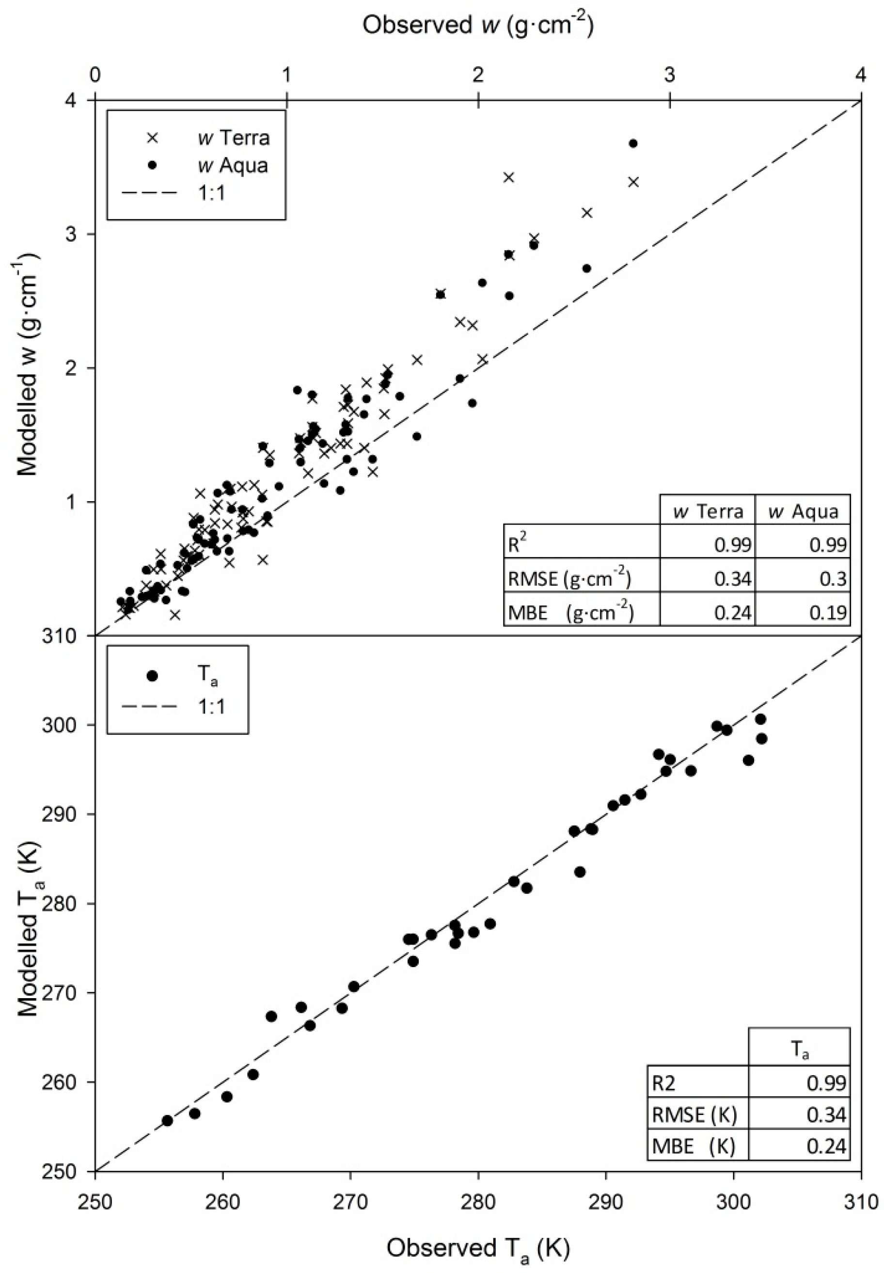
7.1. Air Temperature and Water Vapor Validation

Validation of at-satellite T_a against in situ T_a data for each site yielded an RMSE of 1.7 K and an R² of 0.98 (Figure 5). These results are comparable to those found in [25] when modelling T_a and have an error similar to other studies that used at-satellite T_a for surface temperature and surface energy flux retrieval [17,34]. Results also suggest that the methodology presented by [11] could be applied successfully when in situ T_a measurements are sparse. As shown by the sensitivity analysis, this error could be as high as ~0.4 K in the final surface temperature retrieval which is still well under the acceptable LST retrieval error of less than 1 K. Therefore, the methodology described in [11] to retrieve at-satellite-pass air temperature was used to retrieve LST regionally.

Terra and Aqua MODIS w product validated against in situ water vapor data yielded RMSE of 0.34 g·cm⁻² and 0.30 g·cm⁻², respectively, MBE of 0.24 g·cm⁻² and 0.19 g·cm⁻², respectively, and R² of 0.99 for both cases. These results are similar to those reported by [17] when modeling LST and to those reported by [26] for Terra MODIS w product (MODIS_w) with an error of 0.5 g·cm⁻². Unfortunately, due to the stray light artifacts, methodologies for w retrieval using Landsat-8 thermal bands are not yet accurate, yielding errors around 1 g·cm⁻² [35] that could lead up to more than 1 K if used [28]. Even though the Terra MODIS w product yielded slightly higher error than did Aqua, both of them were within an acceptable w error, in which an error of around 0.3 g·cm⁻² could lead up around 0.4 K in LST retrieval (Figure 3), and were used to retrieve LST regionally.

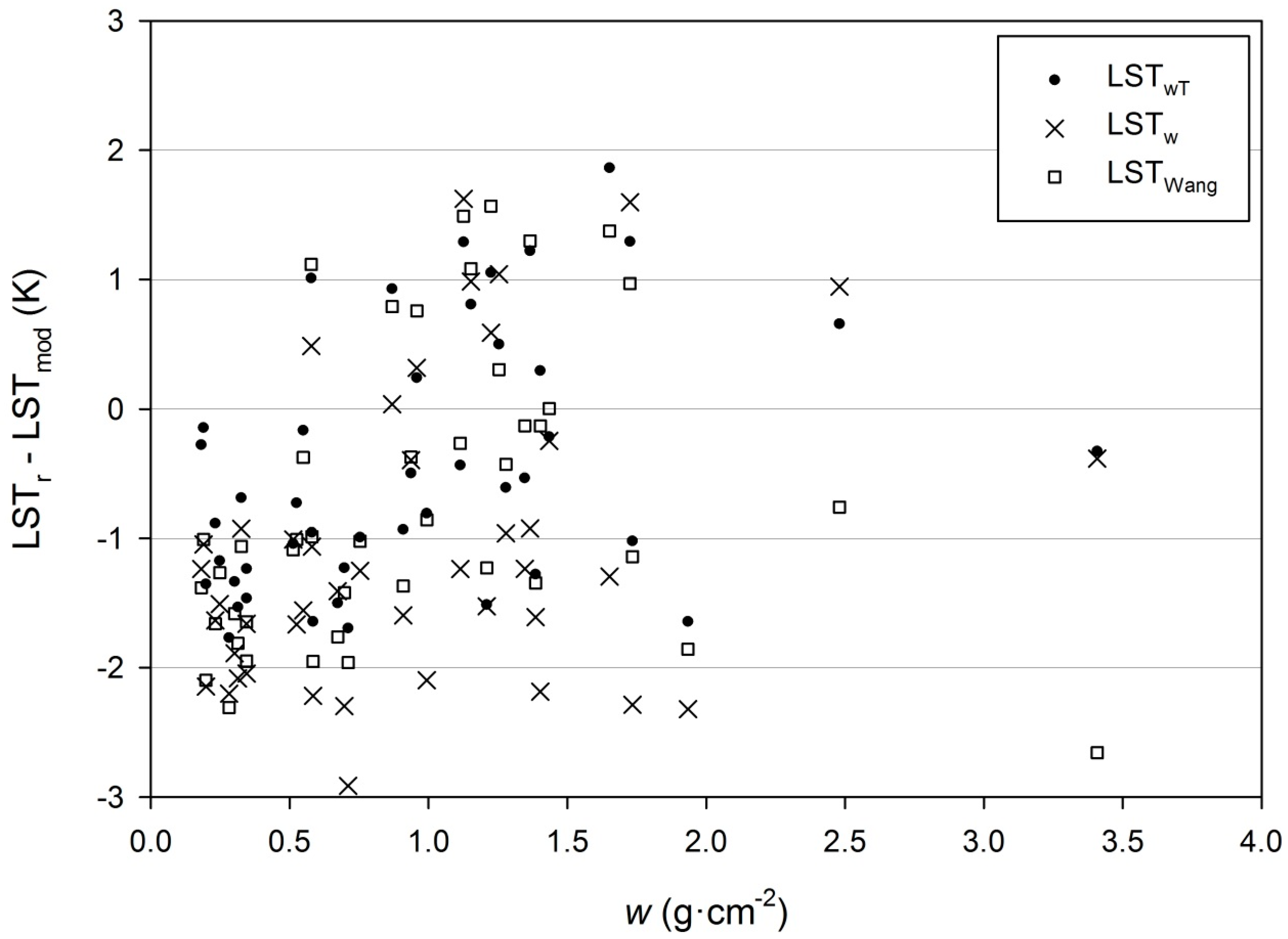
7.2. Land Surface Temperature Validation

LST retrieved using the LST_wT model was validated against in situ data. Additionally, the LST_w model developed using w by [8] and the LST_Wang model developed using T_a and w by [11] were also validated in situ and compared with the LST_wT model. In general, the LST_wT model yielded the best results followed by LST_Wang and LST_w (

Table 3. Accuracy and error statistics from the comparison of modelled vs observed surface temperature. RMSE and MBE are in K. Asterisk is numbers of samples for LST_Wang model.

		LSTwT			LSTw			LSTWang
Cover	n	RMSE	MBE	R2	RMSE	MBE	R2	RMSE	MBE	R2
Snow	17	1.19	−0.97	0.990	1.83	−1.72	0.992	1.55	−1.38	0.989
Vegetation	27/25 *	1.00	−0.15	0.984	1.34	−0.64	0.984	1.19	−0.29	0.975
Total	44/42 *	1.07	−0.47	0.996	1.55	−1.05	0.996	1.34	−0.71	0.992

and Figure 6). These results are also in agreement with [17,19] that found an LST retrieval model improvement when both T_a and w were included as model inputs. The LST_wT model yielded an overall RMSE and MBE of around 1 K and −0.5 K, respectively, while LST_Wang yielded higher RMSE and MBE of 1.35 K and 0.7 K, respectively. Due to LST_Wang model limitations, it was not applied to two images due to lower T_a values than those set in this method. Model performance was also similar to that reported in [17] when comparing LST retrieval methodologies for Landsat-5 TM using both T_a and w as model inputs, yielding better results than [19], the model on which LST_Wang is based. LST_w yielded slightly higher RMSE than LST_Wang but with higher MBE. Besides improving model accuracy, models based also on T_a further decreased model bias. These findings are also in agreement with the simulated data results in which both the RMSE and the MBE are lower when using T_a as a model input (Table 2 and Figure 2). It is also worth noting that regionalized layers of w and T_a, from the MODIS_w product and at-satellite T_a modelled from Daymet data provided robust inputs that helped accurate retrieval of LST at regional scales, as also reported by [17], being particularly important in areas with a sparse network of meteorological and flux observations, such as the Arctic.

In the w range between 0 g·cm⁻² and 3.5 g·cm⁻², the difference between LST_r and LST_wT that remains mainly between -1 K and 1 K was around 60% (Figure 6), while for LST_w and LST_Wang was around 30%. These results are in line with the sensitivity analysis (Figure 3) in which for LST_w (based on w) the error tends to exceed the −1 K and 1 K interval as w steadily increases, while for LST_wT (based on w and T_a) the model tends to be within this range. However, LST_Wang performed more like LST_w than like LST _wT.

All models yielded better results for vegetation rather than for snow, with LST_wT showing the best accuracy, yielding a lower RMSE of around 0.5 K and being less biased compared to LST_w or LST_Wang. The different performance in snow and vegetation covers might be due to the use of a constant surface emissivity for snow. Because of the current lack of an operative method to compute surface emissivity in snow and ice, this was then set to 0.985, and it might be increasing the error in LST retrieval. Unfortunately, there is limited information of LST evaluation for this cover using Landsat-8 TIRS data. However, bias errors for LST_wT found in this study are in agreement with those found by [36], of around 0.6 ± 2 °C when validating Terra and Aqua LST in Barrow, Alaska, in a tundra snow site using Thermocron data. Validation over vegetation showed a behavior similar to snow but with lower RMSE and MBE, yielding the best results for LST_wT, followed by LST_Wang and LST_w. Furthermore, compared with other studies using Band 10, the LST_wT method also yielded better results. An RMSE and an MBE of 1.11 K and −0.93 K, respectively, using pyrgeometer data from four SURFRAD experimental sites in USA and a total of four Landsat images were reported [37] when applying the LST_w method. Using the same method and SURFRAD experimental sites in USA and 44 Landsat-8 images for model validation, an RMSE and an MBE of 1.56 K and −0.73 K, respectively, were reported [38]. Finally, an RMSE and an MBE for the LST_Wang model of 0.67 K and 0.43 K using 11 simulated situations with 3 and 8 different w and T_a values, for mid-latitude winter, summer, and tropical standard atmospheres, respectively, were found in [11]. LST_wT evaluation with simulated data (Table 2) yielded slightly higher RMSE but lower MBE; however, in the present study evaluation a larger radiosonde dataset (a total of 1994 radiosondes) covering a wider range of w and T_a were used. Moreover, it is important to note that when in situ data was used for model validation, LST_wT showed superior performance. When evaluating both LST_Wang and LST_w with simulated data [11], LST_w yielded an RMSE of 1.05 K and an MBE of −2.86 K. However, the RMSE found in this study for LST_w was around 0.7 K higher than for models using both w and T_a, for either in situ or simulated data, but MBE never exceeded 1 K—far from what [11] reported.

8. Conclusions

An improved single-channel method to retrieve LST from Landsat-8 TIRS Band 10 using T_a and w as input data, based on a previous single-channel model applied to atmospherically correct Landsat TM and ETM+ thermal data, was successfully parameterized and evaluated with simulated data from a global and robust radiosonde database, the GAPRI₄₇₁₄, and validated with in situ data from four flux tower sites that included different types of vegetation and snow cover in 44 Landsat-8 scenes. Evaluation results using simulated data showed that the inclusion of T_a together with w within a single-channel scheme improves LST retrieval, yielding lower errors and less bias than models based only on w. Similar results were found when validating the new model presented in this study and three other LST retrieval models against in situ data. The new proposed LST retrieval model, developed with both w and T_a, yielded overall errors on the order of 1 K and a bias of −0.5 K. When validated for vegetation, the model provided lower errors and less bias of −1 K and −0.15 K, respectively; while those for snow had an error of 1.19 K and a bias of −0.97 K, respectively. Despite this difference, which might be caused by the use of a constant value of land surface emissivity for the snow cover, retrieval of LST in vegetation and snow covers showed better performance than other models parameterized using w and T_a or only w that yielded higher RMSE and more bias. However, it is worth noting than when T_a is not available, LST retrieval using only w is still a robust choice when the atmospheric w is low or intermediate.

Finally, at-satellite T_a models and the Terra and Aqua MODIS w product have proven to be robust inputs to retrieve LST regionally. This circumvents the need to rely on radiosonde data, which is a significant achievement for studying the Arctic and other areas that have a sparse network of meteorological observations.

References

1. Kustas, W.; Anderson, M. Advances in thermal infrared remote sensing for land surface modeling. Agric. For. Meteorol. 2009, 149, 2071–2081. [Google Scholar] [CrossRef]
2. Cristóbal, J.; Prakash, A.; Anderson, M.C.; Kustas, W.P.; Euskirchen, E.S.; Kane, D.L. Estimation of surface energy fluxes in the arctic tundra using the remote sensing thermal-based two-source energy balance model. Hydrol. Earth Syst. Sci. 2017, 21, 1339–1358. [Google Scholar] [CrossRef]
3. Li, Z.L.; Tang, B.H.; Wu, H.; Ren, H.Z.; Yan, G.J.; Wan, Z.M.; Trigo, I.F.; Sobrino, J.A. Satellite-derived land surface temperature: Current status and perspectives. Remote Sens. Environ. 2013, 131, 14–37. [Google Scholar] [CrossRef]
4. Reuter, D.; Richardson, C.; Pellerano, F.; Irons, J.; Allen, R.; Anderson, M.; Jhabvala, M.; Lunsford, A.; Montanaro, M.; Smith, R.; et al. The thermal infrared sensor (TIRS) on landsat 8: Design overview and pre-launch characterization. Remote Sens. 2015, 7, 1135–1153. [Google Scholar] [CrossRef]
5. Wan, Z.; Li, Z.L. Radiance-based validation of the v5 modis land-surface temperature product. Int. J. Remote Sens. 2008, 29, 5373–5395. [Google Scholar] [CrossRef]
6. Jin, M.; Li, J.; Wang, C.; Shang, R. A practical split-window algorithm for retrieving land surface temperature from landsat-8 data and a case study of an urban area in China. Remote Sens. 2015, 7, 4371–4390. [Google Scholar] [CrossRef]
7. Rozenstein, O.; Qin, Z.; Derimian, Y.; Karnieli, A. Derivation of land surface temperature for landsat-8 tirs using a split window algorithm. Sensors 2014, 14, 5768–5780. [Google Scholar] [CrossRef] [PubMed]
8. Jimenez-Munoz, J.C.; Sobrino, J.A.; Skokovic, D.; Mattar, C.; Cristobal, J. Land surface temperature retrieval methods from landsat-8 thermal infrared sensor data. IEEE Geosci. Remote Sens. Lett. 2014, 11, 1840–1843. [Google Scholar] [CrossRef]
9. Tardy, B.; Rivalland, V.; Huc, M.; Hagolle, O.; Marcq, S.; Boulet, G. A software tool for atmospheric correction and surface temperature estimation of landsat infrared thermal data. Remote Sens. 2016, 8, 696. [Google Scholar] [CrossRef] [Green Version]
10. Rosas, J.; Houborg, R.; McCabe, M. Sensitivity of landsat 8 surface temperature estimates to atmospheric profile data: A study using modtran in dryland irrigated systems. Remote Sens. 2017, 9, 988. [Google Scholar]
11. Wang, F.; Qin, Z.; Song, C.; Tu, L.; Karnieli, A.; Zhao, S. An improved mono-window algorithm for land surface temperature retrieval from landsat 8 thermal infrared sensor data. Remote Sens. 2015, 7, 4268–4289. [Google Scholar] [CrossRef]
12. Montanaro, M.; Gerace, A.; Lunsford, A.; Reuter, D. Stray light artifacts in imagery from the landsat 8 thermal infrared sensor. Remote Sens. 2014, 6, 10435–10456. [Google Scholar] [CrossRef]
13. Barsi, J.; Schott, J.; Hook, S.; Raqueno, N.; Markham, B.; Radocinski, R. Landsat-8 thermal infrared sensor (tirs) vicarious radiometric calibration. Remote Sens. 2014, 6, 11607–11626. [Google Scholar] [CrossRef]
14. Gerace, A.; Montanaro, M. Derivation and validation of the stray light correction algorithm for the thermal infrared sensor onboard landsat 8. Remote Sens. Environ. 2017, 191, 246–257. [Google Scholar] [CrossRef]
15. Barsi, J.A.; Barker, J.L.; Schott, J.R. An atmospheric Correction Parameter Calculator for a Single Thermal Band Earth-Sensing Instrument. In Proceedings of the 2003 IEEE International Geoscience and Remote Sensing Symposium (IEEE Cat. No.03CH37477), Toulouse, France, 21–25 July 2003; pp. 3014–3016. [Google Scholar]
16. Barsi, J.A.; Schott, J.R.; Palluconi, F.D.; Hook, S.J. Validation of a web-based atmospheric correction tool for single thermal band instruments. In Proceedings of the Optics and Photonics 2005, San Diego, CA, USA, 22 August 2005; p. 7. [Google Scholar]
17. Cristóbal, J.; Jiménez-Muñoz, J.C.; Sobrino, J.A.; Ninyerola, M.; Pons, X. Improvements in land surface temperature retrieval from the landsat series thermal band using water vapor and air temperature. J. Geophys. Res. 2009, 114. [Google Scholar] [CrossRef]
18. Mattar, C.; Duran-Alarcon, C.; Jimenez-Munoz, J.C.; Santamaria-Artigas, A.; Olivera-Guerra, L.; Sobrino, J.A. Global atmospheric profiles from reanalysis information (GAPRI): A new database for earth surface temperature retrieval. Int. J. Remote Sens. 2015, 36, 5045–5060. [Google Scholar] [CrossRef]
19. Qin, Z.; Karnieli, A.; Berliner, P. A mono-window algorithm for retrieving land surface temperature from landsat tm data and its application to the israel-egypt border region. Int. J. Remote Sens. 2001, 22, 3719–3746. [Google Scholar] [CrossRef]
20. Jiménez-Muñoz, J.C.; Sobrino, J.A. A generalized single-channel method for retrieving land surface temperature from remote sensing data. J. Geophys. Res. Atmos. 2003, 108. [Google Scholar] [CrossRef]
21. Jimenez-Munoz, J.C.; Cristobal, J.; Sobrino, J.A.; Soria, G.; Ninyerola, M.; Pons, X. Revision of the single-channel algorithm for land surface temperature retrieval from landsat thermal-infrared data. IEEE Trans. Geosci. Remote 2009, 47, 339–349. [Google Scholar] [CrossRef]
22. Chedin, A.; Scott, N.A.; Wahiche, C.; Moulinier, P. The improved initialization inversion method: A high resolution physical method for temperature retrievals from satellites of the tiros-n series. J. Clim. Appl. Meteorol. 1985, 24, 128–143. [Google Scholar] [CrossRef]
23. Chevallier, F.; Chéruy, F.; Scott, N.A.; Chédin, A. A neural network approach for a fast and accurate computation of a longwave radiative budget. J. Appl. Meteorol. 1998, 37, 1385–1397. [Google Scholar] [CrossRef]
24. Aires, F.; Chédin, A.; Scott, N.A.; Rossow, W.B. A regularized neural net approach for retrieval of atmospheric and surface temperatures with the iasi instrument. J. Appl. Meteorol. 2002, 41, 144–159. [Google Scholar] [CrossRef]
25. Cristóbal, J.; Ninyerola, M.; Pons, X. Modeling air temperature through a combination of remote sensing and gis data. J. Geophys. Res. 2008, 113, 1–13. [Google Scholar] [CrossRef]
26. Sobrino, J.A.; El Kharraz, J.; Li, Z.L. Surface temperature and water vapour retrieval from modis data. Int. J. Remote Sens. 2003, 24, 5161–5182. [Google Scholar] [CrossRef]
27. Li, Z.-L.; Jia, L.; Su, Z.; Wan, Z.; Zhang, R. A new approach for retrieving precipitable water from ATSR2 split-window channel data over land area. Int. J. Remote Sens. 2003, 24, 5095–5117. [Google Scholar] [CrossRef]
28. Jiménez-Muñoz, J.C.; Sobrino, J.A. Error sources on the land surface temperature retrieved from thermal infrared single channel remote sensing data. Int. J. Remote Sens. 2006, 27, 999–1014. [Google Scholar] [CrossRef]
29. Wang, K.C.; Liang, S.L. Evaluation of aster and modis land surface temperature and emissivity products using long-term surface longwave radiation observations at surfrad sites. Remote Sens. Environ. 2009, 113, 1556–1565. [Google Scholar] [CrossRef]
30. Cristóbal, J.; Graham, P.; Buchhorn, M.; Prakash, A. A new integrated high-latitude thermal laboratory for the characterization of land surface processes in alaska’s arctic and boreal regions. Data 2016, 1, 13. [Google Scholar] [CrossRef]
31. Pons, X.; Pesquer, L.; Cristóbal, J.; González-Guerrero, O. Automatic and improved radiometric correction of landsat imagery using reference values from modis surface reflectance images. Int. J. Appl. Earth Obs. 2014, 33, 243–254. [Google Scholar] [CrossRef]
32. Sobrino, J.A.; Jimenez-Munoz, J.C.; Soria, G.; Romaguera, M.; Guanter, L.; Moreno, J.; Plaza, A.; Martincz, P. Land surface emissivity retrieval from different vnir and tir sensors. IEEE Trans. Geosci. Remote 2008, 46, 316–327. [Google Scholar] [CrossRef]
33. Thornton, P.E.; Thornton, M.M.; Mayer, B.W.; Wei, Y.; Devarakonda, R.; Vose, R.S.; Cook, R.B. Daymet: Daily Surface Weather Data on a 1-km Grid for North America; Version 3; ORNL DAAC: Oak Ridge, TN, USA, 2017. [Google Scholar]
34. Cristóbal, J.; Poyatos, R.; Ninyerola, M.; Llorens, P.; Pons, X. Combining remote sensing and gis climate modelling to estimate daily forest evapotranspiration in a mediterranean mountain area. Hydrol. Earth Syst. Sci. 2011, 15, 1563–1575. [Google Scholar] [CrossRef]
35. Ren, H.; Du, C.; Liu, R.; Qin, Q.; Yan, G.; Li, Z.-L.; Meng, J. Atmospheric water vapor retrieval from landsat 8 thermal infrared images. J. Geophys. Res. Atmos. 2015, 120, 1723–1738. [Google Scholar] [CrossRef]
36. Hall, D.K.; Nghiem, S.V.; Rigor, I.G.; Miller, J.A. Uncertainties of temperature measurements on snow-covered land and sea ice from in situ and modis data during bromex. J. Appl. Meteorol. Clim. 2015, 54, 966–978. [Google Scholar] [CrossRef]
37. Zhang, Z.; He, G.; Wang, M.; Long, T.; Wang, G.; Zhang, X.; Jiao, W. Towards an operational method for land surface temperature retrieval from landsat 8 data. Remote Sens. Lett. 2016, 7, 279–288. [Google Scholar] [CrossRef]
38. Yu, X.; Guo, X.; Wu, Z. Land surface temperature retrieval from landsat 8 TIRS—Comparison between radiative transfer equation-based method, split window algorithm and single channel method. Remote Sens. 2014, 6, 9829–9852. [Google Scholar] [CrossRef]
Figure 1. Spatial distribution of the Global Atmospheric Profiles from Reanalysis Information (GAPRI4714) radiosonde database.
Remotesensing 10 00431 g001
Figure 2. Differences between reference LST (LSTr) and modeled LST (in K) using GAPRI4714 as the atmospheric radiosonde database and w and Ta as input data. LSTw is the model developed using only w, LSTwT is the new model developed using both w and Ta.
Remotesensing 10 00431 g002
Figure 3. Errors in land surface temperature (LST) due to errors in w and Ta.
Remotesensing 10 00431 g003
Figure 4. Location of the validation sites in the study area. Panel A is the Barrow coastal tundra Atmospheric Radiation Measurement (ARM) site; Panel B is the Oliktok coastal tundra ARM site; Panel C is the flux tower site at University of Alaska Fairbanks (UAF); and Panel D is the flux tower site at Caribou-Poker Creeks Research Watershed (CPCRW).
Remotesensing 10 00431 g004
Figure 5. Comparison of modelled vs observed w (top panel) and Ta (bottom panel). The 1:1 line represents perfect agreement with observations.
Remotesensing 10 00431 g005
Figure 6. Differences between reference LST (LSTr) and modelled LST (LSTmod) in K, using Terra and Aqua w and modelled Ta as input data. LSTw is the model developed using only w, LSTwT is the model developed using both w and Ta, and LSTWang is the model developed by [11].
Remotesensing 10 00431 g006